Chrono CDI: Coherent diffractive imaging of time-evolving samples

In this case, the simulated data $D_{t}^{\rm sim}$ is generated by 3D Fourier transforms of each complex valued Pd nanocube reconstruction in the time series after zero padding to meet the oversampling (OS) requirements of phase retrieval [20]. We refer to an oversampling of 2 as the required oversampling (Req. O.S.). In practice, this means the cube size was half of the array size in all three dimensions. The time sequence considered consists of $t=0,12,18,26,34,42,50,58,66$, and $76$ minutes. This time sequence is approximately equally spaced and, as shown in Fig. 2, has varying amounts of nearest-neighbor correlation, with an average nearest-neighbor correlation coefficient of 61%. The correlation coefficient $c(t,t^{\prime})\in[-1,1]$ is defined between two 3D displacement fields at time states $t$ and $t^{\prime}$ by

where $u_{111}$ is the displacement field projection and $\bar{u}_{111}$ is the average displacement field over the particle.

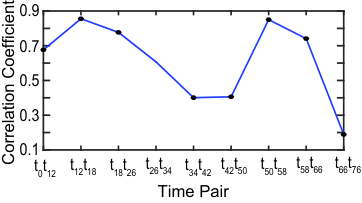
Figure 3a shows the correlation coefficient matrix for the chosen time sequence. Figure 2 is a plot of the super-diagonal matrix values. The chosen time sequence is a good balance between having smooth evolution between nearest neighbors and having a large change over the whole time sequence (both the displacement and the amplitude change significantly). The first numerical test of chrono CDI reconstructs the sequence $\rho_{t}$ from the sequence of $D_{t}^{\rm sim}$ with the required oversampling.

The algorithm uses with random initial starts and alternates between the error reduction (ER) and the hybrid input-output (HIO) algorithms using a feedback parameter of $\beta=0.7$ [21]; the support is fixed to the size of the object and is not evolved during the iterative process. At iteration numbers $N=100n$, for $n=1,2,\ldots,18$, the algorithm tests whether all reconstructions are correctly oriented with respect to the known initial ($t=0$ minutes) and final ($t=76$ minutes) states by testing whether they are conjugated and reflected (“twin”) solutions [21]. Although reconstructing the “twin” image does not affect $\varepsilon_{\scalebox{0.5}{$\mathcal{M}$}}^{2}$, it will negatively impact $\mu$, resulting in an artificially high total objective. One constraint used in the present work is that the $\rho_{t}$ of the initial and final states are known in real and diffraction space. This constraint can be achieved by measuring diffraction datasets at the required oversampling before the experimental dynamics start and after no significant changes are seen in the diffraction data.

Figure 3b shows the errors $\varepsilon_{\scalebox{0.5}{$\mathcal{M}$}}^{2}(\rho_{t},D^{\rm sim}_{t})$ and $\mu(\rho_{t},\rho_{t^{\prime}})$, averaged over all reconstructed time states and over 10 random starts, as a function of the scalar weight $w$. Both errors are normalized by the total intensity in the image. Figure  in the Supplemental Material shows the modulus error $\varepsilon_{\scalebox{0.5}{$\mathcal{M}$}}^{2}$ as a function of iteration number for two scalar weight values. The initial and final states ($t=0$ and $t=76$ minutes, respectively) are known in real space. When $w=0$, the modulus error is the lowest, and the miscorrelation term is the largest. These results are expected because the data is noise-free and oversampled at the required oversampling such that a unique solution is fully determined for each $D_{t}^{\rm sim}$. The weight $w=0$ corresponds to the case when no correlations are taken into account. As $w$ increases, $\mu(\rho_{t},\rho_{t^{\prime}})$ decreases, and $\varepsilon_{\scalebox{0.5}{$\mathcal{M}$}}^{2}$ increases for the solution set $\{\rho_{t}\}$ because their relative contributions to the total objective change. With data sampled at the required oversampling, including information from neighboring time steps in a time series will not improve each individual reconstruction because the complete 3D structural description of the sample at each time is uniquely encoded in the 3D coherent intensity pattern.

We now explore how the additional redundancy from the time series can compensate for reduced oversampling during the rocking curve (e.g. oversampling at less than a factor of 2) at a given time step by reconstructing the time series $D_{t}^{\rm sim}$ discussed previously but with different degrees of reduced sampling in $q_{z}$. To start, every third 2D diffraction measurement of the original 84 2D diffraction measurements was selected to form $D_{t}^{\rm sim}$ for all times except the initial and final time. This leads to data that has 1/3 of the required oversampling. If such a time series were measured experimentally, the measurement time would be reduced by a factor of 3. In assessing algorithm performance, the modulus error was calculated by comparing the far-field exit wave of the reconstructions with the data sampled at the required oversampling. As before, the initial and final states are known, the support is known, and alternating ER/HIO is used as described previously.

Figure 4a shows the average (over all time states and random starts) modulus error as a function of the scalar weight $w$ for varying amounts of oversampling. The average normalized modulus error does not change from $w=0$ to $w=10^{-4}$. Unlike the results using the required oversampling (shown in Fig. 3b) where the lowest modulus error occurs for $w=0$ (no time correlation), in the cases where $q_{z}$ has been sampled at 1/3 (blue) and 1/20 (black) of the required oversampling, a minimum in the modulus error is observed at a value of $w=0.01$. This modulus error is computed with respect to the datasets that are sampled at the required oversampling, and thus the reconstructions at these minima are the “best” solutions. When only 1/84 (red) of the required oversampling is used (i.e., a single slice from the rocking curve), the modulus error decreases with increasing $w$ and approaches a constant value, which is near the normalized average modulus error when all the reconstructed time states are set to the average of the initial and final state (black dashed horizontal line). In this case, simply using an average of the initial and final states outperforms the reconstruction algorithm, indicating that there are insufficient reciprocal space constraints and that the oversampling in $q_{z}$ is too low.

On average $w=0.01$ improves the reconstructed time sequence relative to $w=0$, which takes no time correlation into account, for up to 1/20 of the required oversampling. However, it is not clear from the plot of the average whether all time states are being improved equally. Figure 4b shows the normalized modulus error at each time state for $w=0,0.01,0.5$ at 1/3 of the required oversampling for a particular random start. The states nearest to the known states ($t=0$ and $t=76$ minutes) have lower modulus errors, as expected. By comparing $w=0$ with $w=0.01$, we see that the improvement occurs in all the intermediate states except the state at $t=66$ minutes, which remains essentially unchanged. These results demonstrate that the algorithm improves all reconstructions, even those least correlated with their neighbors (see Fig. 2 for a plot of the nearest neighbor correlation). The benefits of chrono CDI are clear when the required oversampling is reduced by up to a factor of approximately 1/20. In these cases, enforcing a degree of nearest-time-step, real-space correlation provides an additional constraint that improves the reconstruction at all intermediate times relative to what can be achieved using conventional phase retrieval.

We now demonstrate chrono CDI on experimental rocking curve data. To simulate varying degrees of reduced oversampling, a subset of the original 2D measurements was selected from the experimental datasets. Figure 5 shows example 2D experimental diffraction measurements from the Pd (111) Bragg rocking curve; see Ulvestad, et al. [13] for more details. An oversampling of approximately 3 in $q_{z}$ was used during the original measurement. The reconstruction algorithm is the same as described previously except that the support is not known a priori. Instead, an initial box half the array size in each dimension is used, and the support is updated with the shrinkwrap algorithm [22, 14] using a Gaussian function with a threshold of $0.01$ and standard deviation of 1.

Figure 6 shows chrono CDI reconstructions for two representative time states of experimental diffraction data from Pd nanocubes undergoing structural transformations when exposed to hydrogen gas. As before, different amounts of oversampling were investigated. The isosurfaces shown correspond to the reconstructed Bragg electron density, while the color map corresponds to the image phase $\phi$, which is proportional to the $u_{111}$ displacement field. Figure 6a shows reconstructions when 1/2 of the required oversampling in $q_{z}$ is used. Every third slice of the original data (oversampled at a factor of 3 in $q_{z}$) was used to generate data. This corresponds to an oversampling of 1, which is 1/2 the required oversampling of 2. The reconstruction for $w=0.01$ is much improved compared with $w=0$ and is similar in morphology and lattice displacement to the true solution. Figure 6b shows that the same conclusion holds for $t=42$ minutes. See Figure  in the Supplemental Material for central cross-sections that show the amplitude and phase distributions inside the crystal. The average normalized modulus error of the time sequence is improved from $0.2$ to $0.1$ by including nearest-neighbor information (via $w=0.01$). Although the reconstructions do not match exactly, the results convey the same overall physical changes in the crystal.

Figure 7 shows that when 3/10 of the required oversampling is used (corresponding to every 5th slice of the original data), major differences in both the reconstructed Bragg electron density and displacement fields arise as compared with the full-rocking-curve reconstructions. There are also disagreements in the reconstructed phases (proportional to the displacements). We therefore conclude that chrono CDI applied to this particular set of measurement data for the chosen time sequence could have decreased the measurement time by a factor of 2 without losing the essential physics of the transforming crystal. For simulated data it could have reduced the time by up to a factor of 20. The discrepancy is likely due to the finite extent in reciprocal space of the real data, noise in the data, and the unknown support that must be determined via the shrinkwrap algorithm during the reconstruction.

References

- [1] M. A. Pfeifer, G. J. Williams, I. A. Vartanyants, R. Harder, and I. K. Robinson, Nature 442, 63 (2006).
- [2] I. Robinson and R. Harder, Nature Materials 8, 291 (2009).
- [3] A. Ulvestad, A. Singer, J. N. Clark, H. M. Cho, J. W. Kim, R. Harder, J. Maser, Y. S. Meng, and O. G. Shpyrko, Science 348, 1344 (2015a).
- [4] J. N. Clark, J. Ihli, A. S. Schenk, Y.-y. Kim, A. N. Kulak, M. Campbell, G. Nisbit, F. C. Meldrum, and I. K. Robinson, Nature Materials 14, 780 (2015).
- [5] A. Ulvestad, A. Singer, H.-M. Cho, J. N. Clark, R. Harder, J. Maser, Y. S. Meng, and O. G. Shpyrko, Nano Letters 14, 5123 (2014).
- [6] A. Ulvestad, J. N. Clark, A. Singer, D. Vine, H. M. Cho, R. Harder, Y. S. Meng, and O. G. Shpyrko, Physical Chemistry Chemical Physics 17, 10551 (2015b).
- [7] W. Cha, N. C. Jeong, S. Song, H.-j. Park, T. C. Thanh Pham, R. Harder, B. Lim, G. Xiong, D. Ahn, I. McNulty, J. Kim, K. B. Yoon, I. K. Robinson, and H. Kim, Nature Materials 12, 729 (2013).
- [8] M. Watari, R. A. McKendry, M. Vögtli, G. Aeppli, Y.-A. Soh, X. Shi, G. Xiong, X. Huang, R. Harder, and I. K. Robinson, Nature Materials 10, 862 (2011).
- [9] A. Ulvestad, J. N. Clark, R. Harder, I. K. Robinson, and O. G. Shpyrko, Nano Letters 15, 40664070 (2015c).
- [10] X. Huang, W. Yang, R. Harder, Y. Sun, M. Lu, Y. S. Chu, I. K. Robinson, and H. kwang Mao, Nano Letters 15, 7644 (2015).
- [11] G. Xiong, J. N. Clark, C. Nicklin, J. Rawle, and I. K. Robinson, Scientific Reports 4, 6765 (2014).
- [12] J. N. Clark, L. Beitra, G. Xiong, A. Higginbotham, D. M. Fritz, H. T. Lemke, D. Zhu, M. Chollet, G. J. Williams, M. Messerschmidt, B. Abbey, R. J. Harder, A. M. Korsunsky, J. S. Wark, and I. K. Robinson, Science 341, 56 (2013).
- [13] A. Ulvestad, M. J. Welland, S. S. E. Collins, R. Harder, E. Maxey, J. Wingert, A. Singer, S. Hy, P. Mulvaney, P. Zapol, and O. G. Shpyrko, Nature Communications 6, 10092 (2015d).
- [14] H. N. Chapman, A. Barty, and S. Marchesini, Journal of the Optical Society of America A 23, 1179 (2006).
- [15] M. C. Newton, S. J. Leake, R. Harder, and I. K. Robinson, Nature Materials 9, 120 (2010).
- [16] E. Wicke and H. Brodowsky, Hydrogen in palladium and palladium alloys, Vol. 21 (1996) pp. 461–464.
- [17] T. B. Flanagan and W. A. Oates, Annual Review of Materials Science 21, 269 (1991).
- [18] S. Marchesini, Review of Scientific Instruments 78, 011301 (2007).
- [19] A. Tripathi, S. Leyffer, T. Munson, and S. M. Wild, Procedia Computer Science 51, 815 (2015).
- [20] F. Livet, Acta Crystallographica Section A: Foundations of Crystallography 63, 87 (2007).
- [21] J. R. Fienup, C. C. Wackerman, and A. Arbor, Journal of the Optical Society of America A 3, 1897 (1986).
- [22] S. Marchesini, H. He, H. N. Chapman, S. P. Hau-Riege, A. Noy, M. R. Howells, U. Weierstall, and J. C. H. Spence, Physical Review B 68, 140101 (2003).
- [23] K. Mohan, S. Venkatakrishnan, J. Gibbs, E. Gulsoy, X. Xiao, M. De Graef, P. Voorhees, and C. Bouman, IEEE Transactions on Computational Imaging 9403, 1 (2015).
- [24] J. W. Gibbs, K. A. Mohan, E. B. Gulsoy, A. J. Shahani, X. Xiao, C. A. Bouman, M. De Graef, and P. W. Voorhees, Scientific Reports 5, 11824 (2015).
- [25] J. Bø Fløystad, E. T. B. Skjønsfjell, M. Guizar-Sicairos, K. Høydalsvik, J. He, J. W. Andreasen, Z. Zhang, and D. W. Breiby, Advanced Engineering Materials 17, 545 (2015).
- [26] S. O. Hruszkewycz, M. J. Highland, M. V. Holt, D. Kim, C. M. Folkman, C. Thompson, A. Tripathi, G. B. Stephenson, S. Hong, and P. H. Fuoss, Physical Review Letters 110, 177601 (2013).
- [27] A. Tripathi, J. Mohanty, S. H. Dietze, O. G. Shpyrko, E. Shipton, E. E. Fullerton, S. S. Kim, and I. McNulty, Proceedings of the National Academy of Sciences of the United States of America 108, 13393 (2011).