On the Gravitational stability of gravito-turbulent accretion disks
Abstract
Low mass, self-gravitating accretion disks admit quasi-steady, ‘gravito-turbulent’ states in which cooling balances turbulent viscous heating. However, numerical simulations show that gravito-turbulence cannot be sustained beyond dynamical timescales when the cooling rate or corresponding turbulent viscosity is too large. The result is disk fragmentation. We motivate and quantify an interpretation of disk fragmentation as the inability to maintain gravito-turbulence due to formal secondary instabilities driven by:
1) cooling, which reduces pressure support; and/or 2) viscosity, which reduces rotational support.We analyze the axisymmetric gravitational stability of viscous, non-adiabatic accretion disks with internal heating, external irradiation, and cooling in the shearing box approximation. We consider parameterized cooling functions in 2D and 3D disks, as well as radiative diffusion in 3D. We show that generally there is no critical cooling rate/viscosity below which the disk is formally stable, although interesting limits appear for unstable modes with lengthscales on the order of the disk thickness. We apply this new linear theory to protoplanetary disks subject to gravito-turbulence modeled as an effective viscosity, and cooling regulated by dust opacity. We find that viscosity renders the disk beyond AU dynamically unstable on radial lengthscales a few times the local disk thickness. This is coincident with the empirical condition for disk fragmentation based on a maximum sustainable stress. We suggest turbulent stresses can play an active role in realistic disk fragmentation by removing rotational stabilization against self-gravity, and that the observed transition in behavior from gravito-turbulent to fragmenting may reflect instability of the gravito-turbulent state itself.
I. Introduction
Understanding the gravitational stability of rotating disks is central to many astrophysical problems [26]. In the context of gaseous protostellar or protoplanetary disks (PPDs), gravitational instability (GI) has two applications. It can provide gravitational torques to transport angular momentum outwards and thus enable mass accretion [2, 68]. GI may also lead to disk fragmentation, which has been invoked to explain the formation of stellar/sub-stellar companions or giant planets at large radii [7, 27, 64, 19] Studying these non-linear phenomena requires direct numerical simulations. Nevertheless, physical insight can be obtained through analytical modeling.
The standard metric for the (inverse) strength of disk self-gravity is the Toomre parameter,
| (1) |
[67]. Here, is the isothermal sound-speed, is the epicyclic frequency (which equals the rotation frequency in a Keplerian disk), is the surface density and is the gravitational constant. The Toomre parameter is a measure of the destabilizing effect of self-gravity () against the stabilizing effect of rotation () and pressure (). This is evident from the dispersion relation,
| (2) |
which relates the growth rate and radial wavenumber for local, axisymmetric waves in a two-dimensional (2D, razor-thin), inviscid and isothermal11 1 Eq. 1—2 also apply to adiabatic disks if one takes as the adiabatic sound-speed. disk. When , there is a range of for which such disturbances are unstable. Non-axisymmetric modes can develop for larger, but still order-unity values of [32, 51, 50].
We emphasize that the oft-used dispersion relation and corresponding Toomre parameter (Eqs. 1 and 2) are derived from idealized conditions: the base disk is laminar, inviscid, and does not experience any net thermal losses22 2 Isothermal disks implicitly assume heating and thermal losses are exactly balanced at all times, so these do not cool in the current context. (hereafter ‘cooling’). However, real disks can cool, for example, due to radiative losses. Accretion disks may also be turbulent, the dynamic and thermodynamic effect of which is often modeled through an effective viscosity [58, 36, 3, 53].
However, the Toomre parameter is still widely applied to viscous (turbulent), cooling accretion disk models [15, 10, 25, e.g.], despite the mismatch in the included underlying physics. We show that including non-ideal physics, such as cooling and viscosity, in fact modifies the classic dispersion relation, and hence the condition for GI. Thus the Toomre condition alone is insufficient to assess GI in realistic disks.
The goal of this work is to generalize the analytic treatment of disk GI, by including cooling and viscosity, to allow a self-consistent discussion of GI in realistic accretion disk models. We first review in §I.1 and §I.2, respectively, how cooling or viscosity can lead to GI even when , by removing pressure or rotational support. We then discuss in §I.3—§I.4 how these effects may relate to the transition from self-regulated GI to fragmentation seen in numerical simulations. The rest of this paper is laid out in §I.5.
I.1. Cooling-driven gravitational instability
Cooling reduces pressure support against self-gravity. The cooling time is the timescale over which the disk temperature is relaxed to some floor value, which may be zero. It is often written as
| (3) |
where is the corresponding dimensionless cooling time. This type of parameterized cooling, first applied by [15], allows a range of thermodynamic responses to be explored.
In reality, PPD cooling is controlled by radiation from dust grains [6, 11, 8]. Although most PPDs subject to GI are optically thick, cooling parameterized by the model formally only captures optically thin cooling when used in numerical simulations. It is, however, possible to modify the standard cooling function to mimic optically-thick cooling (see, e.g. §VI).
Previous work has quantified the role of cooling primarily as a means to reduce the sound speed term in [9, though see e.g.,]. Here we will quantify how cooling enables GI even when . For example, if perturbations can cool to arbitrarily low temperatures (which, in fact, is a common cooling prescription in numerical simulations), we find the above dispersion relation is modified to read
| (4) |
where is the adiabatic index. Cooling increases the growth rate by reducing the magnitude of the pressure term. In fact, for a formal condition for instability is
which is what would be obtained from Eq. 2 with pressure neglected (). This condition does not actually depend on the cooling time, and instability is possible for any finite . Thus, the mere presence of cooling changes the qualitative nature of GI compared to the simple Toomre condition.
I.2. Viscosity-driven gravitational instability
Viscous disks can also develop GI even when . This is because, as demonstrated below, viscosity removes rotational support against self-gravity for long-wavelength disturbances [42, 70, 14]. A similar effect occurs in dusty fluids where the required frictional forces are provided by dust-gas drag [18, 69, 66]. In fact, this is a mechanism to enhance particle clumping for planetesimal formation [71, 72]. Therefore it is not unreasonable to expect analogous fragmentation in gaseous disks due to viscosity.
It is conventional to write the kinematic viscosity as
| (5) |
where is the dimensionless viscosity coefficient [58]. This parameterization can be modified to include more complex dependencies on the fluid variables, but Eq. 5 is the general form.
For an isothermal, viscous, self-gravitating disk in 2D, [14] finds the approximate dispersion relation
| (6) |
Assuming , instability occurs if
provided that . This condition for viscous GI is identical to what would be obtained from Eq. 2 with rotation neglected (). That is, a classically stable disk can be destabilized by viscosity as it reduces rotational stabilization [42].
For gaseous accretion disks, a Navier-Stokes viscosity is often implemented (as above) to mimic hydrodynamic or magneto-hydrodynamic (MHD) turbulence [58]. How well turbulence can be modeled as an effective viscosity is a separate issue [5]. However, it is reasonable to assume that these mechanisms, which are observed in simulations to transport angular momentum outwards (and mass inwards), frustrate rotational support.
In this work, we use viscosity to model two possible physical effects of turbulence: heating via dissipation and angular momentum transport. We emphasize that our model for GI enabled by viscosity (hereafter viscous GI) does not assume a particular origin for the viscosity. GI itself or other forms of magnetic or hydrodynamic turbulence are allowed in this framework. We will generalize the theory of viscous GI to include an energy equation with viscous heating, irradiation, explicit cooling, as well as three-dimensionality (3D) in order to consider viscous GI in more realistic PPD models.
I.3. Relevance to gravito-turbulent disk fragmentation
We develop a general framework for viscous disks without assuming a specific origin for the viscosity. We will, however, apply the theory to ‘gravito-turbulent’ disks in which the viscosity is associated with some underlying (classic) GI, as described below.
Consider an initially laminar, disk, without external heating, as it cools. The disk temperature will decline until , whence non-axisymmetric modes grow and heat the disk through the dissipation of spiral shocks [10]. This setup permits a quasi-steady, turbulent state with in which cooling is balanced by shock heating to maintain thermal equilibrium [15, 59].
Global disk simulations [40, e.g.] show that the transport and heating associated with this gravito-turbulence may be described as a local viscous process provided that the disk-to-star mass ratio is small () and the disk is thin (aspect-ratio ).
In this case the and parameters defined above are inversely related (see, e.g. Eq. 24). Recent vertically-extended shearing box simulations also confirm this relation in 3D disks [59].
Numerical experiments, however, show that if the cooling time is too small (or the viscosity is too large), say,
| (7) |
then the disk fragments [15, 56, 54]. In fact, in the absence of global effects, numerical simulations show that there are two — and only two — possible outcomes for self-gravitating, cooling disks: gravito-turbulence or fragmentation.
There is considerable debate on the exact value of and whether or not a critical cooling time can be defined at all [45, 39, 46, 48, 20]. There are, in addition, numerical convergence issues when simulating disk fragmentation, which we discuss in §VII.
However, it is generally accepted that steady, gravito-turbulent disks do not exist for sufficiently rapid cooling or large viscosity [22]. This is intriguing because, as highlighted in §I.1—I.2, cooling or viscosity can reduce gravitational stability independently of their influence on the exact value of the classic . This motivates a physical interpretation of disk fragmentation as the inability to maintain a gravito-turbulent state due to secondary instabilities driven by cooling and/or viscosity.
I.4. Instability of the gravito-turbulent state
In this work, we formally treat the gravito-turbulent disk described above as an equilibrium state, to which we apply standard linear stability analysis. Thus by ‘perturbations’ we mean deviations away from this gravito-turbulent basic state33 3 This should not be confused with fluctuations with respect to the laminar disk that maintain the underlying gravito-turbulence.. In our model, we interpret instability of such perturbations to signify fragmentation. Although we cannot formally demonstrate this, numerical simulations suggest that gravito-turbulence and fragmentations are the only outcomes of classic GI. Thus the failure to maintain the gravito-turbulent steady state seems a reasonable description of fragmentation.
I.5. Plan
The basic equations, disk equilibria, cooling and viscosity models are given in §II. The linear stability problem is defined in §III. We present results with parameterized ‘beta’ cooling in §IV and §V for 2D and 3D disks, respectively. In §VI we consider PPDs with realistic viscosity/cooling models, including radiative diffusion in 3D, and determine where PPDs are gravitationally unstable and why. We summarize our results in §VII with a discussion of how our models may aid the physical understanding of fragmentation in realistic PPDs.
II. Basic equations
We consider a 3D, self-gravitating, viscous disk with heating and cooling. We use the shearing box framework to study a small patch of the disk [16]. The local frame co-rotates with a fiducial point in the unperturbed disk at angular frequency . The Cartesian co-ordinates correspond to the radial, azimuthal and vertical directions in the global disk. The fluid equations are
| (8) | ||||
| (9) | ||||
| (10) |
where is the density field and is the velocity field. We assume an ideal gas so that the pressure and thermal energy density are related by
| (11) |
where is the gas constant and is the temperature. For simplicity we refer to the adiabatic index as that in Eq. 11 for both 2D and 3D disk models [22, cf.]. The gas gravitational potential is given via the Poisson equation,
| (12) |
In the momentum equation (Eq. 9), the third, fourth/fifth, and last term on the right-hand side represent the Coriolis, tidal, and viscous forces (see below), respectively. We consider Keplerian disks with shear parameter and vertical oscillation frequency .
In the energy equation (Eq. 10) the source terms and represent viscous heating and time-dependent cooling, respectively, and represents any time-independent heat source/sinks. We set unless otherwise stated.
II.1. Viscosity and heating
The Cartesian components of the viscous stress tensor are defined by
| (13) |
where is the shear viscosity. We also include a bulk viscosity for completeness, but will neglect it in numerical calculations. The associated viscous heating is given by
| (14) |
where summation over repeated indices is implied.
We adopt a viscosity law
| (15) |
where subscript ‘eq’ denotes the equilibrium state and . The dimensionless viscosity coefficient characterizes the magnitude of the shear viscosity in steady state. The indices are free parameters chosen to model how the viscosity behaves in the perturbed state. We adopt the same prescription for the bulk viscosity but with .
Our numerical calculations use so that is time-independent, following previous studies of viscous GI [42, 21, 70, 14]. This choice eliminates viscous over-stability [57, 31], which is unrelated to self-gravity, and would otherwise contaminate our results.
While steady-state viscosity values can be determined analytically or numerically [44, 28, 53, e.g.], the time-dependent behavior is not well-explored. We emphasize the choice is made to bring out the physical process of interest — viscous GI. Interestingly, though, [34] have suggested a dependence when modeling the evolution of 2D self-gravitating disks as a viscous process. We note that if is constant in time then increasing the density corresponds to reduction in the viscosity. This is perhaps consistent with numerical simulations of disk fragmentation which show that the internal flow of high-density clumps is laminar [15]. However, once clumps form they may effectively decouple from the background disk state, and thus no longer be described by the same prescription.
II.2. Steady states and cooling models
We consider equilibrium solutions (here omitting the ‘eq’ subscripts for simplicity)
| (16) | ||||
| (17) | ||||
| (18) |
The equilibrium density and pressure fields are obtained by solving the vertical momentum equation with self-gravity,
| (19) | ||||
| (20) |
together with thermodynamic equilibrium,
| (21) |
where the first term represents viscous heating. For the viscous problem, , and we set to obtain a relation between viscous heating and cooling (e.g. Eq. 24 below). However, if we wish to neglect viscosity (and the accompanying dissipation) but include cooling, we must invoke to define an equilibrium state. To proceed further, we separately describe the two cooling models considered in this work.
II.2.1 Beta cooling
In our beta cooling model, the energy loss per unit volume is specified as an explicit function of the thermodynamic variables. A prototypical example is
| (22) |
where is a reference temperature field, and recall is the cooling timescale with a constant input parameter. Physically, may be the floor temperature set by, for example, stellar or background irradiation.
Beta cooling of the form Eq. 22 is widely applied in 2D and 3D numerical simulations of self-gravitating disks [15, 56, 54, 48]. In fact, for the cooling function is identical to that originally employed by [15]. We will refer to Eq. 22 as ‘standard’ beta cooling. It permits numerical experiments to be carried out in a controlled manner as a function of the cooling time . An adiabatic disk corresponds to . The physical meaning of the limit depends on , as discussed in §IV.1.1—IV.1.2.
For standard beta cooling we assume an equilibrium polytropic relation
| (23) |
where is the equilibrium mid-plane density, and is the constant polytropic index that determines the disk’s vertical structure. Thus is only relevant to the 3D problem. The vertical structure is first obtained from Eq. 19—20, then inserted into Eq. 21 to infer the required viscosity profile for thermal equilibrium. If ,
| (24) |
with
| (25) |
where is the equilibrium temperature field. We shall consider vertically isothermal disks with , as appropriate for the outer parts of irradiated protoplanetary disks [8]. In this case , and are simply constants. Note that should only be interpreted as an irradiation parameter when it is defined through Eq. 25, in conjunction with adopting Eq. 22 as the cooling function.
We assume standard beta cooling in formulating the linear problem. However, the corresponding linear problem for any other explicit cooling function, say , can be obtained by equating its linearized form to that of Eq. 22, i.e. setting . This then defines the and parameters to be used in the framework we develop later (see also §III.1). We do this in §VI where we adopt a more realistic beta cooling function for PPDs. In that case, may or may not directly represent a physical irradiation.
II.2.2 Radiative cooling
A more realistic treatment of cooling considers energy transfer by radiative diffusion. Then
| (26) | ||||
| (27) |
where is the Stefan-Boltzmann constant and is the (dust) opacity. We adopt
| (28) |
and take the constant index as appropriate for the cold outer regions of a PPD with ISM-like dust grains [6], but retain the general notation to keep track of the opacity.
In this case, we specify a constant viscosity coefficient and solve Eq. 19—21, together with Eq. 26—27, as a fourth order system of ordinary differential equations to obtain equilibrium profiles , , and hence .
While radiative cooling is arguably more realistic than beta cooling, it generally implies a vertically non-isothermal equilibrium disk, and increases the order of the linearized equations. It formally applies to optically-thick disks, but it is possible to modify the flux function to account for optically-thin disks [35]. However, this complication is beyond the scope of this work.
III. Linear problem
We consider infinitesimal axisymmetric Eulerian perturbations of the form
| (29) |
and equivalent form for other variables. Here, is an input real horizontal wavenumber and is a (generally) complex growth rate. For simplicity, hereafter we drop the tilde.
The linearized continuity, momentum and energy equations are
| (30) | ||||
| (31) | ||||
| (32) | ||||
| (33) | ||||
| (34) | ||||
| (35) |
where ′ denotes . The perturbed viscous forces are
| (36) | ||||
| (37) | ||||
| (38) |
and the perturbed viscous heating is given by
| (39) | ||||
| (40) |
In Eq. 35, the 3D self-gravity parameter is
| (41) |
[43]. The linearized cooling functions are given below. Eq. 30—35, supplemented with appropriate boundary conditions, constitutes an eigenvalue problem for the growth rate .
III.1. Linearized beta cooling
For the standard beta cooling prescription, linearizing Eq. 22 gives
| (42) |
where we have used from the ideal gas law.
Note that any beta cooling function can be linearized in the form of Eq. 42 with appropriate definitions of and (see §VI.2 for an example). For the stability problem we may simply regard as a parameter for the density-dependence of any generic beta cooling function. If we specifically consider standard beta cooling, then also represents physical irradiation.
III.2. Linearized radiative cooling
Linearizing Eq. 26—27 with the temperature-dependent opacity law in Eq. 28 gives
| (43) |
Since Eq. 43 contains vertical derivatives of the perturbations, it is not generically possible to map radiative cooling to the beta cooling prescription, except for special problems [38, e.g.].
We now consider the gravitational stability of two and three dimensional disks in the presence of non-ideal physics: cooling and viscosity.
IV. Two-dimensional disks with beta cooling
We begin in the 2D limit with standard beta cooling to facilitate comparison with previous studies. The disk material is assumed to be confined to the mid-plane, and . We make the replacement , re-interpret as the vertically-integrated pressure, and set . The gravitational potential perturbation remains 3D and its mid-plane value is given by
| (44) |
[61].
The linearized equations yield an algebraic dispersion relation . We write this in terms of the dimensionless growth rate and wavenumber as
| (45) |
where the functions are given in Appendix A. We use this generalized dispersion relation to investigate GI driven by cooling in §IV.1; and GI driven by viscosity in §IV.2.
IV.1. Inviscid limit
We first simplify the problem by setting . This eliminates viscous heating and forces in the linearized problem, allowing us to quantify the sole effect of cooling on the perturbations. We emphasize that destabilization is independent of the effect of decreasing temperature on the instantaneous value of the classic-. A time-independent heat source should be invoked to balance the imposed cooling to allow an equilibrium to be defined ().
For example, we could assume that the viscosity only provides a background heating and does not play an active role in the perturbed state. This is in fact done implicitly in the literature when discussing fragmentation of cooling, self-gravitating disk simulations [15]. There, the effect of the ambient gravito-turbulent viscosity on the forming-clump is neglected, as one only compares adiabatic heating and the imposed cooling. This comparison is encapsulated in the generalized dispersion relation below.
Eq. 45 becomes
| (46) |
similar to the classic dispersion relation (Eq. 2), which may be obtained by taking the limit . The first term on the right-hand-side represents destabilization by self-gravity; the second and third terms represent stabilization by rotation and pressure, respectively. The imposed cooling/irradiation only affects the pressure response.
Eq. 46 is a cubic equation in . The Routh-Hurwitz criteria imply that stability is ensured if
| (47) |
are both satisfied. A third criterion, , is formally required, but this is implied by Eq. 47. Notice these conditions do not actually depend on the cooling time. At fixed , the second stability condition eventually fails for decreasing , i.e. if perturbations are allowed to cool to sufficiently low temperatures.
If only real growth rates are considered, then violating the second condition in Eq. 47 alone is sufficient for instability. In that case the wavenumbers satisfying
| (48) |
are unstable. The range of unstable wavenumbers increases with decreasing irradiation . For this range is . Without irradiation there is no upper limit to unstable wavenumbers, which could have implications for numerical simulations probing large wavenumbers and small scales at high resolution (see §VII.1).
Consider the most unstable wavenumber at which and . By differentiating Eq. 46, we obtain
| (49) |
Inserting this into Eq. 46, we find the maximum growth rate satisfies
| (50) |
Eq. 49—50 imply for . Then as cooling becomes more rapid, the maximum growth rate increases, and the most unstable wavelength decreases. For , Eq. 50 gives the simple solution
| (51) |
Thus as , but growth rates are never zero for any finite . That is, the disk can be formally unstable for arbitrarily long cooling times.
Fig. 1 shows growth rates in a disk as a function of the cooling time for two irradiation levels . The vertical lines mark characteristic cooling times beyond which the growth timescale is long compared to the dynamical time. Increasing irradiation stabilizes the disk, and faster cooling is required to achieve the same growth rate as in a disk with weaker irradiation.

Next, we consider the two limiting cases: , so perturbations are cooled towards zero temperature [15, typically employed in numerical simulations, e.g.]; and , where the equilibrium disk temperature equals the irradiation temperature.
IV.1.1
For -cooling with , the disk is unconditionally unstable for finite , although instability occurs on smaller scales as increases. The limit corresponds to a pressureless disk (not merely isothermal).
Let us consider a disk with
| (52) |
which is the condition for marginal stability in an adiabatic disk. How does finite cooling destabilize the disk? Inserting Eq. 52 into Eq. 50 with , we find
| (53) |
The maximum growth rate, , smoothly increases with decreasing . Notice for this growth rate is faster than the imposed cooling rate .
We can define a characteristic cooling time as that which removes pressure support against self-gravity over the natural lengthscale in the problem, the scale-height . We thus set and find, for the Keplerian disk,
| (54) |
This equation gives similar values of the cooling times below which numerical simulations show dynamical disk fragmentation [15, 56, 54]. These simulations employ the same beta cooling prescription with , and determine the fragmentation boundary, , as a function of the adiabatic index . Table 1 shows rough agreement between and . The match is remarkable, especially with the global 3D simulations of [56], since Eq. 54 is derived for 2D disks in the local limit.
IV.1.2
Standard beta cooling with corresponds to ‘thermal relaxation’: the temperature is restored to its initial value over the cooling time [38, 47]. In this case no additional heat source need be invoked to define an inviscid steady state. From Eq. 47, the instability condition is . This is the same as the classic Toomre condition for an isothermal disk (which may be obtained from Eq. 46 by taking ). In this respect, a fully irradiated disk, in which the equilibrium temperature is set externally, behaves isothermally regardless of the cooling time [15, 22].
IV.2. Viscous disk
We now consider a viscous disk with parameters in our adopted viscosity law, Eq. 15. In the 2D case this implies is constant. We check in Appendix B that our dispersion relation reduces to previous results for viscous GI in the isothermal limit (by taking and ).
It is useful to consider several limiting cases. To see the effect of cooling and irradiation, we simplify the dispersion relation, Eq. 45, by assuming . Then for we find
| (55) |
which coincides with Gammie’s Eq. 18 for vanishing wavenumber. For we find
| (56) |
For a rough measure of the maximum growth rate can be obtained by equating Eq. 55 and 5644 4 If is not small and/or is large then one may just use Eq. 55 to maximize over , see the curve in the bottom panel of Fig. 2. This exercise yields
| (57) |
To compute growth rates numerically, we consider a model with , and given by thermal equilibrium (Eq. 24). Furthermore, we relate the strength of self-gravity and viscosity by
| (58) |
to mimic a gravito-turbulent basic state, where one might expect the dimensionless stress [36].
Fig. 2 shows growth rates as a function of the wavenumber obtained from the dispersion relation Eq. 45. The limiting behavior for small/large are well-captured by Eqs. 55 and 56. Comparing the two panels shows that increasing the irradiation level () suppresses small-scale perturbations.


Fig. 3 shows the maximum growth rate (top panel) and the corresponding wavenumber (bottom panel) as a function of the cooling time for . There is good agreement between numerical growth rates and Eq. 57 for . Eq. 57 gives the limiting behavior for this case as
| (59) |
where we have applied Eq. 24 and 58. The disk is unstable for all , but growth timescales are long ( orbits) for . This region is marked by the vertical dashed-dotted line in Fig. 3. The optimum wavenumber decreases with the cooling time for because larger scales are more resistant to the associated increase in viscous damping. This is evident from the dispersion relation in the large wavenumber limit, Eq. 56, showing increasing viscosity weakens small-scale modes.
Numerical simulations of gravito-turbulent disks show there is a maximum () that can be sustained before fragmentation [56]. We can interpret this result in our linear framework. Suppose it is possible to balance rapid cooling () by generating a large gravito-turbulent heating rate () through a small (second case in Eq. 59). Fig. 3 shows that such a disk would be dynamically unstable with growth rate . This is due to the direct effect of viscous stress promoting instability, rather than cooling. Thus, we do not expect rapidly-cooled, and hence highly turbulent, self-gravitating disks to persist beyond dynamical timescales. We might interpret fragmentation as an instability of the highly viscous state (see §I.4). This is consistent with previous numerical simulations performed by [41].


V. Three-dimensional disks with beta cooling
We confirm the above results in 3D disks with vertical structure. Accounting for the third dimension will weaken gravitational instabilities because the disk mass is spread across some vertical extent. It is possible to incorporate this effect in the previous 2D framework, but doing so introduces an additional ‘softening’ parameter as discussed in Appendix C. It is more direct to solve the 3D eigenvalue problem to avoid such uncertainties. Our numerical approach is outlined in Appendix D.
In the following examples we consider a vertically isothermal disk ( in Eq. 23). Then in the viscous case is vertically constant (Eq. 24). We consider only even modes about the mid-plane, and apply a numerical disk surface at such that .
V.1. Inviscid 3D disk
We consider a 3D inviscid disk with , , and . The 3D gravity parameter is defined by Eq. 41. For such a disk, the corresponding Toomre parameter . Recall , defined by Eq. 52, is the Toomre parameter value such that the 2D disk would be marginally stable in the absence of cooling.
Fig. 4 shows growth rates and the most unstable wavenumbers obtained for this model. We also plot 2D results with the 3D correction as described in Appendix C. The (empirically) chosen value of results in a close match between 2D and 3D growth rates, but the most unstable wavenumber in 3D is somewhat smaller. This offset reflects self-gravity being weakened in the vertical direction: a larger horizontal scale is required to achieve the same strength of self-gravity as the 2D case. Similarly, choosing matches the optimum wavenumbers, but growth rates are over-estimated in 2D.


V.2. Viscous 3D disk
For the 3D viscous problem we use the same set up as that in 2D (§IV.2), but with
| (60) |
where is the 3D equivalent to the 2D critical value, . Note that the background vertical structure now varies with through Eq. 60, which in turn depends on the cooling time through thermal equilibrium (Eq. 24).
Fig. 5 shows growth rates, maximized over , as a function of the cooling time . We also plot 2D results with 3D corrections. Softening the self-gravity in 2D captures the correct qualitative behavior of the full 3D case. For choosing produces a good match. However, it is clear that a single, constant value of cannot re-produce 3D growth rates for all . This suggests that the exact value of is problem-dependent, although taking should give the correct 3D growth rate within a factor of two.
Fig. 6 shows the magnitude of the vertical velocity scaled by the total horizontal velocity for and . Vertical speeds are sub-dominant at of the total horizontal speeds. These vertical velocities are associated with viscous GI, and should not be compared with those associated with the underlying gravito-turbulence [59, e.g.]. Vertical velocities are formally neglected in our framework when defining the basic state (§II.2).


VI. Application to protoplanetary disks
We now apply our linear framework to assess the stability of PPDs. We consider the gravito-turbulent disk models recently developed by Rafikov [53, hereafter R15 ]. This 2D, Keplerian disk orbits a Solar mass star and is defined by the following parameters,
- •
, the global radial mass accretion rate;
- •
, the value of the 2D Toomre parameter where the disk is gravito-turbulent;
- •
, the irradiation temperature;
- •
These properties serve as inputs for calculating thermal equilibrium, and mass and angular momentum conservation. Together with an opacity law, they allow us to construct a global disk model with surface density and temperature where is the global cylindrical radius from the star. [See 53, for details.] These profiles give , required for input into our linear framework. We derive other dimensionless parameters below.
Although our disk is global in extent, here we consider the local stability at each radius. We are thus neglecting any global instabilities [1, 41, 30] as well as any evolution of the disk properties in response to GI.
VI.1. Effective
In a steady, viscously accreting Keplerian disk with constant we have, approximately, . Hence
| (61) |
which sets the viscosity coefficient to be used at each radius. Note that the disk profiles employed here give constant rather than constant .
VI.2. PPD beta cooling
Energy loss in 53 is given by
| (62) |
per unit area, where
| (63) |
and
| (64) |
is the optical depth. Recall Eq. 28 is our opacity model where with . Eq. 63 accounts for cooling in the optically-thin () and optically-thick () regimes.
Note that Eq. 62 falls within our definition of a beta cooling prescription, because it is an explicit function of the thermodynamic states. However, we formulated the linear problem with the standard beta cooling function given by Eq. 22, which has a different (less realistic) dependence on disk temperature. In order to adapt the existing framework to the above PPD cooling function, we need to identify the equivalent and parameters that are required for the linearized equations (see §III.1).
Linearizing Eq. 62 gives
| (65) |
where
| (66) | ||||
| (67) | ||||
| (68) |
Comparing Eq. 65 with the linearized form of the standard cooling function, Eq. 42, we identify
| (69) | ||||
| (70) |
to be used in the 2D dispersion relation (Eq. 45). Eq. 69 represents a physical cooling time for the perturbations, and is consistent with previous definitions within factors of order unity [e.g. 30, their Eq. 2].
Eq. 70 shows that is related to the true irradiation temperature through the function given by Eq. 68, and is therefore a only a weak function of the irradiation temperature. More specifically for all , and for our adopted opacity law, Eq. 28,
Thus for we have by considering . However, for we have , as expected intuitively.
VI.3. Inviscid stability condition
With our new linearized cooling function in hand, from the discussion in §IV.1 and by applying Eq. 47, we conclude that without viscous effects the disk is stable everywhere if
| (71) |
are both satisfied.
PPDs become irradiation-dominated at large distances from the star, where and [8, 11, 29]. Then Eq. 71 relaxes to in the outer disk. The condition on is then guaranteed. On the other hand, numerical simulations of gravito-turbulence show that [15, 54], and the second inequality is generally satisfied. Taken together, this suggests that in the outer regions of a realistic PPD, cooling may not be the primary cause for a secondary instability of a gravito-turbulent disk, leading to fragmentation. This leaves viscous GI as the only possible culprit within our framework, as we illustrate below.
VI.4. Example 2D calculation
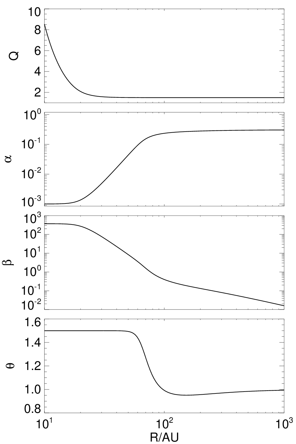
We relax the inviscid assumption and consider a fiducial disk model with , , , and . Such a high accretion rate is consistent with those expected for young protostellar disks [62, 12]. Similarly, is a conservatively low background irradiation level consistent with cloud temperatures in star forming regions [52, 23]. Stellar irradiation will typically elevate in addition to adding a radial dependence [28] We adopt the opacity scale as in 53. We use , approximately applicable to an ideal molecular gas at low temperatures This choice of satisfies the global inviscid stability condition (Eq. 71). Fig. 7 shows the equilibrium disk profile in terms of , , , and . These profiles serve as input to the 2D dispersion relation (Eq. 45, Eq. A1—A5).
Fig. 8 shows growth timescales and optimum wavenumbers for viscous GI in this fiducial model. For comparison we also plot a case with lower accretion rate, ; and analytic estimates based on Eq. 55 (instead of Eq. 57 since here ) which gives the optimum wavenumber and growth rates as
| (72) |
These are similar to the isothermal results of Sterzik et al. [65, their Eq. 19 and 21, respectively], and identical if one takes .
The most unstable wavelength is a few times the disk thickness. So long as , this result is consistent with our use of the local approximation. For our fiducial disk, around AU, and throughout the disk. The increase in from to is due to the decrease in , while that from to occurs as the disk transitions from the optically-thick to optically-thin regime. The mismatch between the numerical and analytic solutions at large distances is expected since the above expressions assume . Nevertheless the analytic estimates reproduce qualitatively correct behavior.
The fiducial disk is subject to viscous GI on dynamical timescales ( orbits) for AU. We note this transition radius is also implied by Eq. 16 in [30]. Coincidentally, beyond this radius (and ), which is often quoted as a condition for disk fragmentation [53, e.g.]. Thus viscous GI may be responsible for the transition between gravito-turbulence and fragmentation due to the removal of rotational support by viscous (turbulent) stresses.
On the other hand, the lower model also attain beyond AU, but everywhere. Applying empirical cooling conditions for fragmentation may then lead to contradiction. Instead, if viscosity is the physical cause for fragmentation, then our result suggest the lower disk should not fragment (at least much less likely than our fiducial case) because the instability cannot develop on orbital timescales.


VI.5. 3D PPD with radiative diffusion
We briefly consider 3D PPDs with explicit radiative diffusion (§II.2.2). Given the and profiles obtained from the 2D model above, at each radius we obtain the vertical structure from Eq. 19—21, with Eq. 26—27 for the radiative flux. We then solve the 3D eigenvalue problem as in §V, with the additional boundary condition that the disk surface temperature is fixed, . We use the fiducial disk model as in §VI.4 but with , since our simple radiative diffusion treatment does not include irradiation (§II.2.2). We use a slightly smaller vertical domain with .
Fig. 9 shows the growth rates and most unstable wavenumber for AU; along with the corresponding 2D results matched with softened self-gravity. There is good agreement for AU where the disk is optically thick () and thus both models apply. However, beyond AU where the disk becomes optically-thin, radiative diffusion (the 3D curve) is not valid and under-estimates the growth rates. Nevertheless, the transition radius of AU, beyond which growth timescales become dynamical, can be correctly calculated within the 2D framework.


VII. Summary and discussion
In this paper, we develop the linear theory of cooling, irradiated, and viscous accretion disks in order to understand gravitational instability (GI) in realistic protoplanetary disks (PPDs). We use a Navier-Stokes viscosity to mimic the effects of turbulent angular momentum transport. This viscosity provides a background heating to balance the imposed cooling, and may also act on linear perturbations. We suggest that disk fragmentation observed in numerical simulations can be understood as the eventual outcome of secondary instabilities of a gravito-turbulent base state, driven by cooling and/or viscosity.
Previous work has focused on the impact of viscosity and cooling on the equilibrium temperature and surface density of an accretion disk, but merely used this to calculate the classic Toomre , thereby assess stability. We demonstrate by explicitly including these effects into the dispersion relation that they can drive secondary instabilities. While viscosity and cooling can be related through thermal balance, they independently enhance growth rates: cooling reduces thermal stabilization; and viscous forces compromise rotational stabilization. This provides a physical explanation as to why rapidly-cooled, gravito-turbulent disks cannot exist. Moreover, we discuss below how these models may lend support to the varied behavior observed in numerical simulations.
The effect of cooling and irradiation on GI is quantified by the dispersion relation Eq. 46. We find sufficient conditions for stability which depends on the irradiation level (Eq. 47) but is independent of the cooling time. This means that long cooling times can still formally lead to instability. However, growth timescales may be uninterestingly long for cooling times . Because cooling affects pressure support, GI driven by cooling occur on small scales, .
We generalize the ‘viscous gravitational instability’, previously studied in isothermal disks [42, 70, 14], to include cooling, viscous heating and irradiation. We consider a disk with viscosity and self-gravity inversely related () to model a gravito-turbulent background, and find viscous GI occurs on orbital timescales for . This is consistent with the notion of a maximum stress sustainable by gravito-turbulence established by numerical simulations [56]. Because viscosity affects rotational support, viscous GI occurs on large scales, . Furthermore, irradiation preferentially stabilizes small-scale perturbations.
We apply our linear framework to protoplanetary disks with realistic models for cooling and gravito-turbulence. We show that with a physically motivated cooling model for PPDs, cooling alone does not lead to gravitational instabilities. This is due to stabilization by an effective ‘irradiation’ associated with the density-dependence of the PPD cooling function as it appears in the stability problem, which is present even if there is no physical irradiation. This captures the fact that density enhancements impede cooling.
Instead, viscous GI occur on dynamical timescales in a PPD for AU because there. This corresponds to a Toomre and a cooling time . These are coincident with empirical conditions cited in the literature to determine disk fragmentation [53, e.g.]. Here, we attribute a physical cause for the fragmentation of realistic PPDs: gravito-turbulent PPDs fragment when turbulent stresses are large enough to further destabilize the disk against self-gravity.
VII.1. Relation to numerical simulations
Our results may help understand some numerical simulations concerning disk fragmentation. Table 1 shows a close match between the characteristic cooling time for cooling-driven GI (Eq. 54) and that for disk fragmentation observed in simulations [15, 56, 54]. This suggests that, at least for those simulations, fragmentation is physically due to the removal of thermal stabilization by cooling on radial lengthscales of the disk thickness. In this interpretation, gravito-turbulence only provides a background heating. Our characteristic cooling time corresponds to a dimensionless background viscosity as defined in the above studies55 5 This differs from our definition of by a factor of .
| (73) |
This is roughly constant, consistent with [56].
More recent simulations have raised the issue of numerical convergence. [45] found that better resolved disks fragmented at longer cooling times. Follow-up studies attributed at least some of this effect to decreasing numerical viscous heating at higher resolution, which helps fragmentation [39, 46]. We can expect this if numerical viscosity contributes to an effective irradiation, because then perturbations can cool to lower temperatures with increasing resolution, see Fig. 1. In global simulations, non-convergence has also been attributed to initial conditions that lead to internal edges [49], but this cannot be modeled in our local setup. [55] point out that the standard implementation of beta cooling in smoothed-particle hydrodynamics (SPH) applies cooling on scales well-below the SPH smoothing lengths, and that this inconsistency may contribute to non-convergence.
However, [48] also found in local 2D grid-based simulations that fragmentation can occur for slowly-cooled disks with , but that this requires simulations to run for significantly longer than dynamical timescales. This is consistent with our finding that for either cooling-driven or viscous GI, there is no critical cooling rate/viscosity below which the disk is formally stable. Instead, growth rates smoothly decrease with increasing (decreasing ), implying that instabilities, and hence fragmentation, simply take longer to develop for slowly-cooled disks. However, to properly consider long timescales, it may be necessary to account for secular evolution in the global disk.
Here, we highlight that most numerical experiments, including those above, employ the standard beta cooling function, Eq. 22, without a physical floor temperature. We show in §IV.1 (see also §I.1) that this implies cooling-driven GI can occur at any sufficiently small scale. Therefore as the numerical resolution increases, simulations can access a wider range of unstable scales. Although small-scale modes have weaker growth rates, they can become important over long timescales. In this respect, it is perhaps not surprising to find non-convergence with increasing resolution and/or integration times. On the other hand, the convergence issue may be less serious in 3D since small-scale modes are more stable in 3D than in 2D (Appendix C).
We suggest having a physical floor temperature in the standard beta cooling prescription is necessary for numerical convergence. This limits the relevant scales to a finite range. Furthermore, without a floor temperature, standard beta cooling is a function of the pressure/energy density field only. There may be some inconsistency in applying results obtained from this to actual PPDs where cooling depends on two thermodynamic states (e.g. pressure and temperature). A floor temperature permits a mapping between standard beta cooling and PPD cooling (§VI.2). Moreover, the standard beta cooling does not account for optical depth effects, which force the mid-plane and high density perturbations to cool more slowly.
A temperature floor may be a necessary, but not sufficient condition for numerical convergence. [4] included a floor temperature in their local 2D simulations but still find that at fixed cooling rates, disks eventually fragment with sufficient spatial resolution. In light of our results on viscous GI, we suggest another possible contribution to non-convergence: high resolution enables small-scale turbulent angular momentum transport to aid clump formation via the removal of rotational support. (See also §VII.2 below.) If clumps are only marginally resolved, simulations may not have sufficient dynamic range for turbulent eddies to cascade down to these scales.
We comment that although modern simulations resolve the dominant scale associated with gravito-turbulence very well, [10], this does not necessarily imply small-scale dynamics/thermodynamics are unimportant [73, especially for non-linear evolution, ], as is evident from the non-converging simulations described above. Even at very high resolution one might worry that the artificial dissipation scale imposed by the grid/smoothing length is too similar to the scale of fragmentation.
VII.2. MHD turbulence
We emphasize that the linear framework we have developed does not assume a particular origin for the turbulence that is represented by the imposed viscosity. For example, our 2D dispersion relation, Eq. 45 with Eq. A1—A5, treats as an independent input parameter.
Our models may thus apply to self-gravitating disks dominated by MHD turbulence. Explicit numerical simulations of magnetized, massive disks have been performed by [13]. This study finds disk fragmentation with increasing numerical resolution, and attributes this to resolving the most unstable MRI wavelength, which enables small-scale angular momentum removal by MHD turbulence to aid fragmentation. This physical mechanism is represented by the viscous GI discussed in this paper, which lends some support for the use of a viscosity to represent turbulence.
VII.3. Outstanding issues
True disk fragmentation is a non-linear process characterized by clumps reaching densities that are orders of magnitude above the ambient value. They must also survive disruption by tidal shear and shocks [60, 74]. Clearly, our linear models cannot address fragmentation directly. Technically, we have only demonstrated that a gravito-turbulent state becomes dynamically unstable, and thus should not persist, when cooling is too rapid or when the associated viscous stresses are too large. However, steady gravito-turbulence or fragmentation are the only possible outcomes of cooling, self-gravitating disks in the local limit [15]. Thus it seems reasonable to speculate that the non-existence of a stable gravito-turbulent state, here due to dynamical instability, implies disk fragmentation.
Our deterministic approach cannot model ‘stochastic fragmentation’ [48, 20]. In this interpretation, fragmentation is attributed to the occurrence and survival of large, non-linear density enhancements, which arise from the gravito-turbulent fluctuations simply by chance. There is insufficient evidence that gravito-turbulence adequately samples the density power spectrum as assumed by [20]. Nevertheless, one might consider this form of fragmentation as a secondary instability triggered by lowering the local Toomre parameter through a (random) increase in density.
The most important assumption in this work is modeling turbulence as a Navier-Stokes viscosity. Furthermore, we have chosen a particular viscosity law (see §II.1) to mimic the effect of turbulence in reducing rotational support (in the sense that it provides small-scale angular momentum transport). How to quantitatively model the effect of gravito- or MHD turbulence as a viscosity, especially on dynamical timescales, should be clarified with direct numerical simulations. The present viscosity models should then be modified accordingly.
Another possible generalization is non-axisymmetric disturbances. In barotropic, inviscid disks non-axisymmetric global GI can develop for somewhat larger than unity [51, 1, 50, 33]. It would be interesting to study how non-axisymmetric perturbations are affected by cooling and viscosity in order to improve the link between disk fragmentation and the stability of gravito-turbulent disks.
We thank the anonymous referee’s prompt report that helped to improve the clarity of this work. We thank S. Stahler and A. Youdin for comments during the course of this project; C. Clarke, C. Gammie, and S.-J. Paardekooper for feedback on the first version of this article, and G. Lodato for useful discussions.
Appendix A 2D dispersion relation
The functions in Eq. 45 are
| (A1) | ||||
| (A2) | ||||
| (A3) | ||||
| (A4) |
with
| (A5) |
Note that these equations treat all the parameters as independent (namely , , , , and ).
Appendix B 2D viscous GI
We obtain the dispersion relation for viscous GI described by previous authors [42, 70, 14] as follows. We set in Eq. 15 to obtain the same viscosity models. Next we consider , i.e. no explicit cooling on the perturbations. Then the condition implies
| (B1) |
which agrees with the above studies in the isothermal limit [; see also 57, their Eq. 28]. The non-isothermal term originates from viscous dissipation, which was excluded in the aforementioned works. Its effect is to increase the maximum wavenumber for viscous GI.
An approximate solution for the growth rate may be obtained for small by balancing the last two terms,
| (B2) |
which coincides with Gammie’s Eq. 18 for .
Appendix C 3D corrections in 2D theory
The simplest way to mimic the effect of finite disk thickness on gravitational instabilities is to weaken self-gravity by reducing the gravitational constant
| (C1) |
or equivalently . This prescription, derived by [63], is widely applied [72, 66, e.g.]. Here is a measure of the disk thickness. We intuitively expect , but its precise value is not known a priori. We regard as a free parameter of the problem.
Appendix D Numerical method for the 3D eigenvalue problem
We use a pseudo-spectral method to solve the set of ordinary differential equations, Eq. 30—35, on the domain with a parity condition at the mid-plane. We expand in even Chebyshev polynomials,
| (D1) |
and the vertical velocity in odd Chebyshev polynomials,
| (D2) |
where and are the spectral coefficients. The basis functions are chosen to satisfy a reflecting boundary condition at the mid-plane,
| (D3) |
For simplicity we apply a reflecting upper disk boundary,
| (D4) |
and the potential satisfies
| (D5) |
We discretize the equations, including upper disk boundary conditions, over the positive abscissae of the extrema of . This procedure converts the differential equations into a generalized eigenvalue problem, for which we use the standard matrix package LAPACK to solve. We use .
References
- [1] Adams, F. C., Ruden, S. P., & Shu, F. H. 1989, ApJ, 347, 959
- [2] Armitage, P. J. 2011, ARA&A, 49, 195
- [3] Armitage, P. J., Livio, M., & Pringle, J. E. 2001, MNRAS, 324, 705
- [4] Baehr, H., & Klahr, H. 2015, ApJ, 814, 155
- [5] Balbus, S. A., & Papaloizou, J. C. B. 1999, ApJ, 521, 650
- [6] Bell, K. R., & Lin, D. N. C. 1994, ApJ, 427, 987
- [7] Boss, A. P. 1997, Science, 276, 1836
- [8] Chiang, E. I., & Goldreich, P. 1997, ApJ, 490, 368
- [9] Clarke, C. J., Harper-Clark, E., & Lodato, G. 2007, MNRAS, 381, 1543
- [10] Cossins, P., Lodato, G., & Clarke, C. J. 2009, MNRAS, 393, 1157
- [11] D’Alessio, P., Calvet, N., & Hartmann, L. 1997, ApJ, 474, 397
- [12] Enoch, M. L., Evans, N. J., Sargent, A. I., & Glenn, J. 2009, ApJ, 692, 973
- [13] Fromang, S. 2005, A&A, 441, 1
- [14] Gammie, C. F. 1996, ApJ, 457, 355
- [15] —. 2001, ApJ, 553, 174
- [16] Goldreich, P., & Lynden-Bell, D. 1965, MNRAS, 130, 125
- [17] Goldreich, P., & Lynden-Bell, D. 1965, MNRAS, 130, 97
- [18] Goodman, J., & Pindor, B. 2000, Icarus, 148, 537
- [19] Helled, R., Bodenheimer, P., Podolak, M., et al. 2014, Protostars and Planets VI, 643
- [20] Hopkins, P. F., & Christiansen, J. L. 2013, ApJ, 776, 48
- [21] Hunter, Jr., J. H., & Horak, T. 1983, ApJ, 265, 402
- [22] Johnson, B. M., & Gammie, C. F. 2003, ApJ, 597, 131
- [23] Johnstone, D., Fich, M., Mitchell, G. F., & Moriarty-Schieven, G. 2001, ApJ, 559, 307
- [24] Kim, J.-G., Kim, W.-T., Seo, Y. M., & Hong, S. S. 2012, ApJ, 761, 131
- [25] Kimura, S. S., & Tsuribe, T. 2012, PASJ, 64, 116
- [26] Kratter, K. M., & Lodato, G. 2016, ArXiv e-prints, arXiv:1603.01280
- [27] Kratter, K. M., & Matzner, C. D. 2006, MNRAS, 373, 1563
- [28] Kratter, K. M., Matzner, C. D., & Krumholz, M. R. 2008, ApJ, 681, 375
- [29] Kratter, K. M., & Murray-Clay, R. A. 2011, ApJ, 740, 1
- [30] Kratter, K. M., Murray-Clay, R. A., & Youdin, A. N. 2010, ApJ, 710, 1375
- [31] Latter, H. N., & Ogilvie, G. I. 2006, MNRAS, 372, 1829
- [32] Lau, Y. Y., & Bertin, G. 1978, ApJ, 226, 508
- [33] Laughlin, G., Korchagin, V., & Adams, F. C. 1997, ApJ, 477, 410
- [34] Laughlin, G., & Rozyczka, M. 1996, ApJ, 456, 279
- [35] Levermore, C. D., & Pomraning, G. C. 1981, ApJ, 248, 321
- [36] Lin, D. N. C., & Pringle, J. E. 1987, MNRAS, 225, 607
- [37] Lin, M.-K. 2014, ApJ, 790, 13
- [38] Lin, M.-K., & Youdin, A. N. 2015, ApJ, 811, 17
- [39] Lodato, G., & Clarke, C. J. 2011, MNRAS, 413, 2735
- [40] Lodato, G., & Rice, W. K. M. 2004, MNRAS, 351, 630
- [41] —. 2005, MNRAS, 358, 1489
- [42] Lynden-Bell, D., & Pringle, J. E. 1974, MNRAS, 168, 603
- [43] Mamatsashvili, G. R., & Rice, W. K. M. 2010, MNRAS, 406, 2050
- [44] Martin, R. G., & Lubow, S. H. 2011, ApJ, 740, L6
- [45] Meru, F., & Bate, M. R. 2011, MNRAS, 411, L1
- [46] —. 2012, MNRAS, 427, 2022
- [47] Mohandas, G., & Pessah, M. E. 2015, ArXiv e-prints, arXiv:1510.02729
- [48] Paardekooper, S.-J. 2012, MNRAS, 421, 3286
- [49] Paardekooper, S.-J., Baruteau, C., & Meru, F. 2011, MNRAS, 416, L65
- [50] Papaloizou, J. C., & Savonije, G. J. 1991, MNRAS, 248, 353
- [51] Papaloizou, J. C. B., & Lin, D. N. C. 1989, ApJ, 344, 645
- [52] Plume, R., Jaffe, D. T., Evans, N. J., I., Martin-Pintado, J., & Gomez-Gonzalez, J. 1997, ApJ, 476, 730
- [53] Rafikov, R. R. 2015, ApJ, 804, 62
- [54] Rice, W. K. M., Armitage, P. J., Mamatsashvili, G. R., Lodato, G., & Clarke, C. J. 2011, MNRAS, 418, 1356
- [55] Rice, W. K. M., Forgan, D. H., & Armitage, P. J. 2012, MNRAS, 420, 1640
- [56] Rice, W. K. M., Lodato, G., & Armitage, P. J. 2005, MNRAS, 364, L56
- [57] Schmit, U., & Tscharnuter, W. M. 1995, Icarus, 115, 304
- [58] Shakura, N. I., & Sunyaev, R. A. 1973, A&A, 24, 337
- [59] Shi, J.-M., & Chiang, E. 2014, ApJ, 789, 34
- [60] Shlosman, I., & Begelman, M. C. 1987, Nature, 329, 810
- [61] Shu, F. H. 1970, ApJ, 160, 99
- [62] —. 1977, ApJ, 214, 488
- [63] Shu, F. H. 1984, in IAU Colloq. 75: Planetary Rings, ed. R. Greenberg & A. Brahic, 513–561
- [64] Stamatellos, D., & Whitworth, A. P. 2009, MNRAS, 392, 413
- [65] Sterzik, M. F., Herold, H., Ruder, H., & Willerding, E. 1995, P& SS, 43, 259
- [66] Takahashi, S. Z., & Inutsuka, S.-i. 2014, ApJ, 794, 55
- [67] Toomre, A. 1964, ApJ, 139, 1217
- [68] Turner, N. J., Fromang, S., Gammie, C., et al. 2014, Protostars and Planets VI, 411
- [69] Ward, W. R. 2000, On Planetesimal Formation: The Role of Collective Particle Behavior (University of Arizona Press), 75–84
- [70] Willerding, E. 1992, Earth Moon and Planets, 56, 173
- [71] Youdin, A. N. 2005, ArXiv Astrophysics e-prints, astro-ph/0508659
- [72] —. 2011, ApJ, 731, 99
- [73] Young, M. D., & Clarke, C. J. 2015, MNRAS, 451, 3987
- [74] —. 2016, MNRAS, 455, 1438