Improved separation of soft and hard components in multiple Coulomb scattering
Abstract
Evaluation of the angular distribution function of particles scattered in an amorphous medium is improved by deforming the integration path in the Fourier integral representation into the complex plane. That allows us to present the distribution function as a sum of two positive components, soft and hard, the soft component being close to a Gaussian, and the hard component vanishing in the forward direction, while including the Rutherford asymptotics and all the power corrections to it at large scattering angles. Detailed properties of those components, and their interplay at intermediate deflection angles are discussed. Comparison with the Molière theory is given.
Keywords:
multiple scattering, large logarithms, resummationpacs
11.80.LaI Introduction
At passage of ultrarelativistic charged particles through amorphous matter, they undergo multiple, essentially uncorrelated scattering on atoms, typically through small angles. If the target is not too thick, the longitudinal momentum of a high-energy particle may be regarded as conserved. Then, the transport equation depends only on the particle deflection angles, and is exactly solvable by means of Fourier transformation [1]. However, conditions of multiple Coulomb scattering on screened atomic nuclei may require one to separately treat hard and soft contributions to the distribution function, as was first pointed out by Williams [2]. That separation was cast in the form of a large-thickness expansion by Molière [3, 4], subsequently reviewed by Bethe [5], and nowadays is recognized as a standard procedure (see [6, 7, 8]). In modern practice, yet a simplified approach is applied at times, retaining only the Gaussian component with the root mean square angle inferred from Gaussian fits [10], or derived analytically from the Molère theory [11]. But in high-statistics experiments, non-Gaussian “wings” are noticeable even for rather thick targets.
Although Molière’s expansion provides a formal background for the theory, from the physical point of view it is not completely satisfactory. It is known that, in principle, it does not converge (see, e.g., [12]), and yet, is comprised of oscillatory functions of deflection angles, which do not admit independent probabilistic interpretation. At the same time, there were recent phenomenological indications that beyond the central Gaussian region, the distribution function does not immediately switch to the asymptotic power law corresponding to single scattering, but exhibits some transient behavior over a sizable range of angles [13, 14].
In case such a transition region does exist, the best option to compute within it the distribution function would be to resum all the non-Gaussian (at least, power-law) contributions through all orders, as is done in other physical problems (see, e.g., [9]). That typically leads to integral representations for resummed quantities. But in the present case, one can employ to this end a method [5, 6], in which the original Fourier integral representation for the distribution function is extended into the complex plane, and two principally different (vertical and horizontal) parts of the integration path are distinguished. That method so far has never developed to a procedure superior to Molière’s expansion; nonetheless, with some improvements, it can be raised to that status, and provide a different view on behavior of the angular distribution beyond the central region. The key notion here is that integrals over the mentioned parts of the path appear to be positive, and therefore may be interpreted as hard and soft scattering components, coexisting at any scattering angle. Comparison of those components will allow us to determine the width of the transition region between Gaussian and Rutherford regions in the aggregate distribution, and assess the significance of resummation of all the plural hard-scattering contributions.
II Preliminary considerations
II.1 Fourier-Bessel solution of the transport equation
The probability distribution of fast particles scattered through small angles in an amorphous medium, , is governed by the transport equation
| (1) |
where is the differential cross-section of particle scattering on one atom through angle , is the density of atoms in the medium, and the traversed target thickness. Equation (1) conserves the normalization:
| (2) |
Solution of Eq. (1) satisfying the initial condition is obtained by means of Fourier-Bessel transformation:
| (3a) | |||||
| (3b) | |||||
II.2 Thick targets: Molière’s theory
At significant target thickness, the random walk in the plane of deflection angles (which may be viewed as transverse vectors) must reduce to diffusion. In generic integral representations (3) and (4), that comes about as follows: at large , the exponential in their integrands is rapidly decreasing, therefore the contributing or are small, permitting one to expand the exponent to leading order in their values. However, naive expansion in the integrand gives a logarithmically diverging variance , given that the physical differential cross-section of fast charged particle scattering on one atom through large angles obeys the Rutherford asymptotics
| (5) |
with being the particle momentum, the nucleus charge, and the fine structure constant. A more accurate calculation [5] shows that the small- asymptotics of the exponent in (3), (4) involves a factor logarithmically depending on :
| (6) |
and thereby spoiling the Gaussianity of the Fourier-Bessel integral. Here , and the screening angle , with being the atomic radius, characterizes the scale of angles at which the singularity in (5) is tamed.11 1 In terms of the exact scattering differential cross-section , with and , the screening angle expresses as (7) where is the Euler’s constant. This definition [5] differs from the more conventional [4] by terms , but numerically, the difference is small. With definition (7), the right-hand side (rhs) of Eq. (6) is the shortest, facilitating the following calculations. Note, too, that while Eq. (6) was written for pure elastic scattering, inelastic contributions can also be incorporated there [17], just by redefining and . Thus, the diffusion here is anomalous, but only marginally, in the sense that the anomaly is logarithmic instead of a power law. That implies that the distribution function does not approach a Lévy distribution [8], albeit is not strictly Gaussian either.
Ratio essentially measures the target thickness in units of the radiation length :
with , and expressible in terms of , as well [see, e.g., [11], Eq. (42)]. For instance, ratio corresponds to targets of solid materials of a few millimeter thickness. In what follows, we will measure the target thickness in -independent fashion, merely in units of .
Approximation (6) appreciably simplifies the structure of integrals (3), (4), but their evaluation still involves non-trivial aspects. Intuitively, it is clear that the diffusion, at least at typical angles, must be close to Gaussian, although with possible logarithmic deviations. To tackle those, Molière [4] assumed that the typical deflection angle is , with such that the difference of logarithmically large parameters is a constant of the order of unity (conventionally set to be zero). Therewith, is a Lambert (or product logarithm) function, asymptotically equal , and the rhs of (6) rewrites as
where . As long as the logarithmic dependence on the rescaled integration variable in the exponent appears to be inversely proportional to the large parameter , that suggests expanding this part of the exponential into power series and formally integrating termwise:
| (8) |
with
| (9) |
Note that the expansion parameter here is only logarithmically small, but for , i.e., , expansion (8) is reported to work reasonably well [4, 5]. An important consequence of (9) is that for all ,
| (10) |
Hence, functions at are not everywhere positive, and do not admit probabilistic interpretation.
Analyzing integrals (9), one finds that at large , components of (8) behave as , which corresponds to a perfect Gaussian, and , which reflects the Rutherford asymptotics . For , times logarithmic factors (which will be determined below). Further analysis reveals that, in fact, functions for make several oscillations,22 2 That owes to the fact that as increases, factor in the integrand of (9) becomes sharply peaking at . Therewith, at fixed and increasing , integral (9) tends to (11) For , the latter scaling law was quoted in [12]. which are much stronger than the asymptotic power-law “tails”. At moderate , they may cause a spurious warp in between the Gaussian and Rutherford regions. Yet, despite the factor in the denominator in the rhs of (9), functions grow with faster than exponentially [see Eq. (11)]. Therefore, in principle, series (8) diverges, though it may still serve as an asymptotic expansion in the limit .
II.3 Thin targets: Power and logarithmic corrections to the Rutherford asymptotics
Even though at typical angles the number of scatterings in any macroscopic target is very large, at significant deflection angles the distribution function may be determined by just a few hard scatterings. It can thus be useful to expand the distribution function into perturbation series
| (12) |
and study the behavior of its components at large .
The lowest-order terms of (12) are
| (13) | |||||
and
The dominant contribution to the integral term in () comes from neighborhoods of two points: , where may be approximated by a constant, and , where . The corresponding asymptotics of the integral thus equals , but it is exactly canceled by the second term of (). Therefore, to determine the asymptotics of , one has to expand the slowly varying factors in the integrand to higher orders:
| (15) | |||||
Here , and , wherewith
| (16) |
Hence, if one considers a “form factor” , which vanishes at , and tends to a constant as , it appears to be a nonmonotonous function of , and overshoots the latter constant at some intermediate . That salient feature of the multiple Coulomb scattering angular distribution was confirmed experimentally (see [15, 5]).
Similarly, it can be proven that higher-order terms in (12) are all positive and asymptotically scale as
| (17) |
For polar angle distribution
| (18) |
the asymptotics of the leading terms of the expansion is
| (19) |
| (20) |
and generally
| (21) |
Note that the coefficients at logarithms in Eqs. (17), (21) turn out to be sizable already at , and grow with factorially. Thus, at moderately large , it would be advantageous to sum such contributions through all orders. Resummations of that kind are usually carried out via Borel transformation [16]. But in our case, construction of a new integral representation is unnecessary, as long as the original integral representation (3) or (4) is already well suited for that purpose. Below we will derive corresponding resumming expressions directly from integrals (3) and (4).
III Analysis in the complex plane
Since we are interested in the case when the number of collisions is high, the exponent in integrals (3), (4) will generally assume large values. The modern approach to deriving asymptotics of such integrals consists in extending the integral into a complex plane. With an appropriate choice of the integration path, the integrand can be made non-oscillatory, which substantially alleviates derivation of the asymptotics of the integral. In application to multiple Coulomb scattering distributions, such a deformation procedure was first suggested by Bethe (see Appendix A in [5], and also [6]), but served mainly for the purpose of deriving the coefficients of large-angle power asymptotic terms [6], or combining just a few such terms to an expression, which still worked only in a limited domain of (at large ) [5]. Here we are going to handle the entire sequence of asymptotic terms simultaneously, but in order to make it applicable everywhere, the definition of the integration path must be improved. The path extension problem appears to be technically simpler for the projected angle distribution, which was not considered in [5] at all, and which we consider here first.
III.1 Projected angle distribution
The diffusion approximation to Eq. (4) reads (see footnote 1)
| (22) |
where we set . When extending this integral to the plane of complex , it is found that its integrand has a single saddle point obeying the equation
| (23) |
As long as Eq. (23) is transcendental, only its approximate solution can be expressed explicitly, which, though, will suit us at the present stage. We can choose an approximation to the solution of (23), which is strictly imaginary:
| (24) |
with a proviso that this formula is good only for (and , which is usually fulfilled in practice). To illustrate the accuracy of approximation (24), in Fig. 1 it is plotted along with the exact solution of equation
| (25) |
obtained from (23) by neglecting . It clearly indicates that approximation (24) begins to fail for .
The logarithmic factor in the exponent in (22) induces a singularity of the integrand at the origin, coinciding with the lower endpoint of the integration interval. The steepest descent path must then start at the origin, and go toward the saddle point. For simplicity of the resulting integral, though, we direct it strictly along the imaginary axis, rewriting the integration variable as . After reaching a point defined by Eq. (25), the path must turn to the right and proceed along the steepest descent path, but again, for simplicity, we just direct it parallel to the real axis (see Fig. 2). Ultimately, the distribution function splits to a sum of two real-variable integrals:
| (26) |
where
| (27) |
| (28) |

Below we will show that in spite of the admitted simplification of the integration path, integrals (27), (28) can be robustly interpreted as hard and soft scattering components. Our task now is to investigate their properties.
Hard component
Component proves to be positive everywhere, even for an approximate solution of the saddle-point equation, insofar as typical contributing in Eq. (27) are always , entailing . Furthermore, almost everywhere it is tolerable to replace in (27) . That is strictly justified in limits of either large or small : If , that becomes possible because the upper integration limit tends to zero, leaving
| (29) | |||||
If , the sine in (27) can be linearized by virtue of the rapid decrease of factor in the integrand. Therewith, expansion of the rest of the exponential into Maclaurin series yields the Rutherford law (13), along with power corrections to it (beyond the leading logarithmic accuracy):
| (30) | |||||
with being the digamma function. Clearly, integral (27) resums also all the higher power corrections to the Rutherford asymptotics.

The fact that the component vanishes in both extremes and implies that it must peak somewhere in between [see Fig. 3]. From the analysis of integral (27), one generally concludes that the summit of must be reached when , i.e., , which is nothing but Molière’s typical angle. More precisely, that corresponds to the rising slope of the peak, while the maximum is located at a somewhat greater (see Fig. 3). The end of the region where resummation effects are strong may be assessed from equating the Rutherford asymptotic term to the doubled next-to-leading-order power correction in (30): , i.e., , where . Due to the sizable numerical coefficients involved therein, interval
appears to be even wider than the soft central region .
Besides that, it is noteworthy that does not lie between its asymptotes (in particular, it goes well above the Rutherford asymptote). This (or rather the corresponding feature for proven in the next subsection) may be responsible for the empirical controversies mentioned in the Introduction.
Soft component

Next, we inspect the soft component, which is defined by integral (28). This integral is close to Gaussian form, so its fastest dependence on stems from the value of the exponential at the endpoint:
where we used the saddle point equation (23) within the accuracy to which we neglected in Eq. (25). To account for the rest of the -dependence, the simplest way might be to replace in the relation
| (31) |
the relatively slowly varying factor by its value in the origin,
| (32) |
More precisely, the width of is , whereas that of is , which is narrower, but not by a very large factor. So, in practice it would be certainly worth taking into account also the slope of in the origin. That can be implemented to the structure of the leading exponential in Eq. (31) by approximating
| (33) |
with . Combining (31), (24) and (33), we obtain a quasi-Gaussian structure
| (34) |
It resembles the zeroth-order approximation of Molière’s expansion (applied to the projected angle distribution), but has a more precise normalization (32), and yet involves under the logarithm in the denominator of the exponent. Due to the latter dependence, (34) is narrower than Molière’s at , i.e., in fact, at typical angles (see Fig. 4). A narrowing of that kind was empirically found in [15]. Besides that, the integral of (34) over , in contrast to the integral of the zeroth component of Molière’s expansion, is somewhat less than unity, leaving a part of the probability for .

Aggregate distribution
The circumstance that components (27), (28) in decomposition (26) peak at different might potentially lead to appearance of a secondary bump in the aggregate distribution. To check whether this happens in reality, let us first assess the scale at which and become commensurable. For large , that occurs at relatively large , allowing one, oversimplistically, to employ the Rutherford asymptotics for , and equate it to the Gaussian approximation for . Solving the equation in the leading logarithmic approximation yields , which is of the order of the scale at which reaches its maximum. Therefore, around its maximum, is commensurable with , and consequently, the sum (26) needs not develop a secondary peak or bump. That is what actually happens in practice, and is physically natural, because a diffusion process tends to smear out all the features of the probability distribution. (But for the rescaled distribution , as was mentioned in Sec. II.3, such a bump does exist [15, 5].)
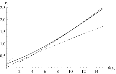
Figure 5 shows the shape of the aggregate distribution, along with contributions to it from different mechanisms, for . The figure demonstrates that the aggregate distribution (solid curve) considerably exceeds the sum of soft and pure Rutherford components (dot-dashed and dotted curves, correspondingly). To account for this excess, one has to employ the resummed hard component (dashed curve) instead of a single-scattering contribution. So, the issue of resummation of plural hard scattering contributions is quite essential in practice. Effectively, it slows down the transition from a Gaussian to Rutherford regime, so that over a substantial angular interval it may mimic a law intermediate between Gaussian and Rutherford decrease, such as a simple exponential law (cf. [13]), or a power law with an index greater than that for the lowest Born approximation, as is the case, e.g., for hard scattering of hadrons (which are themselves composite objects) [14].
Probabilistic interpretation
Granted the positivity of both functions and , in conjunction with the normalization condition , it is tempting further to interpret them independently as partial probability distributions. Specifically, since incorporates all the power-law contributions, it might be regarded as the probability distribution of hard-scattered particles, and , since it is nearly Gaussian, should be interpreted as the probability distribution of soft-scattered particles. That, inevitably, involves an element of arbitrariness, as long as there is no sharp physical boundary between soft- and hard-scattered particles. Besides that, there are regions at sufficiently large , where as evaluated by Eq. (28) becomes slightly negative [though that is immaterial for practice, because there it is already overtaken by ]. For those reasons, it is more appropriate to term the encountered functions pseudo-probability distributions. The mentioned arbitrariness then manifests itself as the residual slight freedom in the choice of the location of the integration path corner.

Accepting the partial (pseudo-)probability interpretation, let us assess the corresponding total probability for a particle to belong to the projected hard component:
| (35) |
At large , inserting (27) to (35) and interchanging the order of integrations leads to
| (36a) | |||||
| The latter single integral can be evaluated by expanding , and integrating termwise, whereupon reassembling it to a single fraction within the given accuracy: | |||||
| (36b) | |||||
That means that essentially, . Formula (36b) shows that the fraction of hard-scattered particles decreases with the increase of the target thickness, as an inverse of its logarithm. The physical reason for this is that the boundary beginning from which the particles must be regarded as hard-scattered moves outwards with the increase of the target thickness, due to the expanding Gaussian component. In contrast, identity (10) in the Molière expansion does not grant direct access to the number of particles in the non-Gaussian component.
The exact behavior of as a function of is plotted in Fig. 6 by the solid curve, along with approximation (36b) plotted by the dashed curve. It appears that (36b) gives a fair approximation for at . It may also be mentioned that the excess of total probability , for and evaluated by approximation (34), (32), with , is positive but small compared with :
That corroborates self-consistency of our approximations.
III.2 Polar angle distribution
Let us next turn to the somewhat subtler case of the polar angle distribution, which is given by Bessel integral (3b). To appropriately extend the corresponding diffusion approximation
| (37) |
to the complex plane of33 3 In [5], was denoted as , but we keep the same notation as for the projected angle distribution. , one needs to substitute in the integrand, and exploit the exponential decrease of Hankel function in the upper half-plane of complex . It is also preferable in the integrand of (37) not to include factor (physically arising as a part of the integration element ) to the expression for which the saddle point is sought. Therewith, the saddle point equation reads
| (38) |
and like in the previous subsection, its solution at large must be predominantly imaginary44 4 That owes to the fact that , like , is an even function of . This would not be the case if the saddle point was sought for the integrand including the factor . The emerging integral representations for and would then be too cumbersome.. Searching a purely imaginary approximation, i.e., letting , utilizing the relation , and neglecting imaginary terms compared to the large real logarithm, leads to a real equation
| (39) |
Unfortunately, now Eq. (39) is difficult to solve by analytic means even approximately, as long as it requires an approximation for applicable at any positive . Simple approximations exist only for large , where , implying
| (40) |
[similar to Eq. (24), and different from Bethe’s choice55 5 In paper [5], the saddle point was actually sought only for part of the integrand, (at real , corresponding to purely imaginary ). Eq. (41) corresponds to effectively replacing under the logarithm by rather than , as is suggested by Eq. (40). That still works when dealing with large-angle asymptotics of the angular distribution, but not when one aims to find a uniform approximation for all deflection angles. In the latter case, the saddle point must be sought for the entire integrand, and the path corner point be chosen as near as possible to it, as is done in the present paper. Moreover, even Eq. (40) may be not the perfect approximation for the entire range of (as we will see below), so, generally, it seems best to solve the corner point equation numerically.
| (41) |
with ], and at small , where , giving in the leading logarithmic approximation
| (42) |
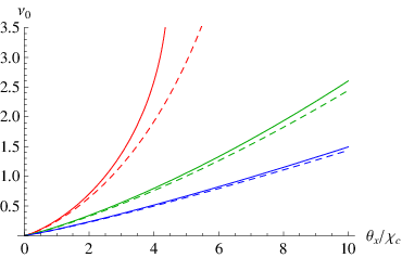
The behavior of the solution of Eq. (39) along with its asymptotes (40), (42) is illustrated in Fig. 7.

Once the solution to Eq. (39) is found, choosing the integration path similarly to that of Fig. 2 leads to a decomposition
| (43) |
with
| (44) |
and
| (45) |
Again, we interpret them as partial pseudoprobability distributions for a particle to belong to hard or to soft scattering probability. Let us now analyze the behavior of those components, and compare them with the corresponding projected angle distributions.

First of all, similarly to the previous subsection, function proves to be everywhere positive, because typical for any are less than unity, and then the sine in the integrand is positive, so we effectively have an integral of a positive definite function. Using the unlimited growth of with , it is straightforward to derive the Rutherford asymptotics for integral (44), along with its next-to-leading order power correction:
| (46) | |||||
The coefficient of the correction term here is in agreement with the leading log calculation (20). In the opposite limit , using (42), function can be shown to decrease much slower than in the case of the projected angle distribution (29):
| (47) | |||||
but tends to zero, anyway. Hence, it must reach a maximum at some finite, nonzero . Figure 8 plots function (44) with evaluated numerically from Eq. (39).
In contrast to the case of projected angle distribution, it appears now that the use of Eq. (40) does not give a good approximation for simultaneously for all typical – because (40) is a much poorer approximation for solution of Eq. (39) itself. That is demonstrated by Fig. 8, where the red curve corresponding to approximation (40) falls much below the calculation with the exact solution of Eq. (39). It signals that for the polar angle distribution, it is much more reliable to solve the corner point equation numerically.
Similarly to the previous subsection, we can find that the support region for function is concentrated at
| (48) |
where .

Equation (39) also does not permit expressing through , which hampers analytic computation of the total pseudoprobability of hard scattering by interchanging the order of integrations. Numerically, of course, that presents no difficulty, and is illustrated in Fig. 9. Qualitatively, function exhibits a behavior similar to that of in Sec. III.1, but is some 3 times greater, so that it cannot be even regarded as small. A satisfactory heuristic approximation of the same structure as Eq. (36b) may be written as
| (49) |
In what concerns , physically it is expected to exhibit a behavior similar to Eq. (34). Indeed, approximation
| (50) |
with
| (51) |
[an integral similar to (36a)] and works reasonably well (see Figs. 10, 11). The total pseudoprobability corresponding to this approximation equals , with (see Fig. 9, red curve), but still tolerably small. Herein, we will restrict our analysis to this notion.

When comparing the results of this subsection with those of Sec. III.1, it should be borne in mind that66 6 Note that in the lhs and in the rhs of Eqs. (52), (53), letter represents different functions.
| (52) |
and correspondingly,
| (53) |
That is clear as long as the integral from a positive function in the rhs of (52) can not vanish at , whereas the left-hand side (lhs) does vanish. It is also natural physically, because hard collisions which are nearly in the -direction are not treated as hard when computing the projected distribution in . But in the large- asymptotics, (52) holds as an equality for all the terms of the descending power series, by virtue of the identity
| (54) |
and its derivatives by index , which generate the logarithmic factors. In turn, inequality (53) explains why constant for approximation (50) is greater than that for approximation (34).
IV Summary
The main conclusions of our paper can be summarized as follows. A continuation into the complex plane allows presenting the angular distribution of probability of particles scattered in amorphous matter as a sum of hard- and soft-scattering components, with no restriction on the number of scatterings. At that, the hard component incorporates all the plural-scattering power-law corrections to the Rutherford single-scattering contribution, while the soft component is nearly Gaussian, but is narrower than Molière’s . Due to their positivity almost everywhere, those components admit independent (pseudo)probabilistic interpretation. The corresponding total percentage of hard-scattered particles (not appearing naturally in the Molière theory) amounts typically for the projected angle distribution, and in case of the polar angle distribution), and sets the accuracy limit for Gauss-like approximations for the soft component.
The second conclusion is that in the aggregate distribution of scattered particles, there is a significant transition region between multiple soft and single hard scattering, in which scattering is multiple but hard. Physically, it is chained to the fact that at significant target thickness, there always exists a range of angles, where the probability of several hard rescatterings is non-negligible. The resummed hard-scattering component peaks at a non-zero deflection angle, and around its maximum (in the so-called semihard region), it exceeds the single hard scattering (Rutherford) contribution by a significant factor. Nonetheless, no bump emerges in the aggregate distribution around this angle, inasmuch as in the semihard region, the hard component is comparable with the soft one.
From the practical point of view, it must be noted that if it is desired to use a single approximation within the central region of scattering angles only, it may be reasonable to employ Molière’s ; but if the hard “tail” needs description, as well, it is advantageous to use the separation introduced herein. Even after approximating by a quasi-Gaussian, the sum is still numerically more accurate than a few first terms of the Molière expansion.
Besides that, it should be remembered that the separation of and somewhat depends on the choice of the corner point for the integration path (which does not coincide with the saddle point of the integrand exactly), and thus may involve slight ambiguity. Analytic solutions of the corner point equation provide insight into qualitative dependencies of the particle distribution function on the total deflection angle and the target thickness, but may sometimes be insufficiently accurate, so, if better precision is required, the saddle point equation is to be solved numerically. Thus, depending on the needs of the study, the proposed construction may be used either for analytic, or for numerical purposes.
References
- [1] W. Bothe, Z. Phys. 5, 63 (1921); G. Wentzel, Ann. Phys. (Leipzig) 69, 335 (1922).
- [2] E.J. Williams, Phys. Rev. 58, 292 (1940).
- [3] G. Molière, Z. Naturforsch. 2a, 133 (1947).
- [4] G. Molière, Z. Naturforsch. 3a, 78 (1948).
- [5] H.A. Bethe, Phys. Rev. 89, 1256 (1953).
- [6] W.T. Scott, Rev. Mod. Phys. 35, 231 (1963).
- [7] N.F. Mott, H.S.W. Massey. The Theory of Atomic Collisions, 3rd ed. Oxford: Clarendon Press, 1965.
- [8] V.V. Uchaikin, V.M. Zolotarev. Chance and Stability. Stable distributions and their applications (Utrecht, VSP, 1999).
- [9] M.V. Bondarenco, Phys. Rev. D 90, 013019 (2014).
- [10] V.L. Highland, Nucl. Instr. Meth. 129, 497 (1975). G.R. Lynch and O.I. Dahl, Nucl. Instr. Meth. B 58, 6 (1991).
- [11] M.V. Bondarenco and N.F. Shul’ga, Phys. Rev. D 90, 116007 (2014).
- [12] A.F. Bielajew, Nucl. Instr. Meth. B 86, 257 (1994).
- [13] A.M. Taratin and W. Scandale, Nucl. Instr. Meth. B 335, 351 (2015).
- [14] F. Arleo, S.J. Brodsky, D.S. Hwang, and A.M. Sickles, Phys. Rev. Lett. 105, 062002 (2010).
- [15] A.O. Hanson et al., Phys. Rev. 84, 634 (1951).
- [16] See, e.g., M. Beneke, Phys. Rep. 317, 1 (1999).
- [17] U. Fano, Phys. Rev. 93, 117 (1954).