Edge Coloring and Stopping Sets Analysis in Product Codes with MDS componentsThanks: This manuscript was submitted to the IEEE Transactions on Information Theory, paper IT-15-1104, Dec. 2015. Fanny Jardel is with Telecom ParisTech, 75013 Paris, France (email: fannjard@gmail.com). She was with CEA, LIST, Communicating Systems Laboratory BC 94, Gif Sur Yvette, F91191, France. Joseph J. Boutros is with the Dept. of Electrical and Computer Engineering, Texas A&M University at Qatar, Education City, 23874 Doha, Qatar (email: boutros@tamu.edu).

Fanny Jardel Joseph J. Boutros Affiliation:

Abstract

We consider non-binary product codes with MDS components and their iterative row-column algebraic decoding on the erasure channel. Both independent and block erasures are considered in this paper. A compact graph representation is introduced on which we define double-diversity edge colorings via the rootcheck concept. An upper bound of the number of decoding iterations is given as a function of the graph size and the color palette size $M$ . Stopping sets are defined in the context of MDS components and a relationship is established with the graph representation. A full characterization of these stopping sets is given up to a size $(d_{1}+1)(d_{2}+1)$ , where $d_{1}$ and $d_{2}$ are the minimum Hamming distances of the column and row MDS components respectively. Then, we propose a differential evolution edge coloring algorithm that produces colorings with a large population of minimal rootcheck order symbols. The complexity of this algorithm per iteration is $o(M^{\aleph})$ , for a given differential evolution parameter $\aleph$ , where $M^{\aleph}$ itself is small with respect to the huge cardinality of the coloring ensemble. The performance of MDS-based product codes with and without double-diversity coloring is analyzed in presence of both block and independent erasures. In the latter case, ML and iterative decoding are proven to coincide at small channel erasure probability. Furthermore, numerical results show excellent performance in presence of unequal erasure probability due to double-diversity colorings.

Index Terms:

Product codes, MDS codes, iterative decoding, codes on graphs, differential evolution, distributive storage, edge coloring, diversity, erasure channel, stopping sets.

I Introduction

The colossal amount of data stored or conveyed by network nodes requires a special design of coding structures to protect information against loss or errors and to facilitate its access. At the end-user level, coding is essential for transmitting information towards the network whether it is located in a single node or distributed over many nodes. At the network level, coding should help nodes to reliably save a big amount of data and to efficiently communicate with each others. Powerful capacity-achieving error-correcting codes developed in the last two decades are mainly efficient at large or asymptotic block length, e.g. low-density parity-check codes (LDPC) [23] and their spatially-coupled ensembles [35], parallel-concatenated convolutional (Turbo) codes [6][5], and polar codes derived from channel polarization [4]. Data transmission and storage in many nowadays networks may require short-length packets that are not suitable for capacity-achieving codes. The current interest in finite-length channel coding rates [44] put back the light on code design for short and moderate block length. Many potential candidates are available for this non-asymptotic length context such as binary and non-binary BCH codes, including Reed-Solomon (RS) codes, Reed-Muller (RM) codes, and tensor product codes of all these linear block codes [40][7][39].

Product codes, introduced by Peter Elias in 1954 [19], are tensor products of two (or more) simple codes with a structure that is well-suited to iterative decoding via its graphical description. In the early decades after their invention, product codes received a great attention due to their capability of correcting multiple burst errors [70][64], the availability of erasure-error bounded-distance decoding algorithms [66], the ability of correcting many errors beyond the guaranteed correction capacity [1], and their efficient implementation with a variable rate [68]. The pioneering work by Tanner [60] brought new tools to coding theory and put codes on graphs, including product codes, and their iterative decoding in the heart of modern coding theory [33][32][49]. The graph approach of coding led to new optimal cycle codes on Ramanujan/Cayley graphs [61] and to Generalizations of LDPC and product codes, known as GLD codes, studied for the binary symmetric channel (BSC) and the Gaussian channel [9]. The excellent performance of iterative (turbo) decoding of product codes on the Gaussian channel [45] made them compete with Turbo codes and LDPC codes for short and moderate block length. The convergence rate and stability of product codes iterative decoding were studied based on a geometric framework [55]. Product codes with mixed convolutional and block components were also found efficient in presence of impulsive noise [22]. In addition, iterated Reed-Muller product codes were shown to exhibit good decoding thresholds for the binary erasure channel, but at high and low coding rates only [65].

The class of product codes in which the row and the column code are both Reed-Solomon codes was extensively used since more than two decades in DVD storage media and in mobile cellular networks [69]. In these systems, the channel is modeled as a symbol-error channel without soft information, i.e. suited to algebraic decoding. Improvements were suggested for these RS-based product codes such as soft information provided by list decoding [52] within the iterative process in a Reddy-Robinson framework [48]. Also, RS-based product codes were directly decoded via a Guruswami-Sudan list decoder [28] after being generalized to bivariate polynomials [3]. For general tensor products of codes and interleaved, a recent efficient list decoding algorithm was published [24], with an improved list size in the binary case. On channels with soft information, RS-based product codes may be row-column decoded with soft-decision constituent decoders [20][30].

Tolhuizen found the Hamming weight distribution of both binary and non-binary product codes up to a weight less than $d_{1}d_{2}+\max(d_{1}\lceil d_{2}/q\rceil,d_{2}\lceil d_{1}/q\rceil)$ [62]. Enumeration of erasure patterns up to a weight less than $d_{1}d_{2}+\min(d_{1},d_{2})$ was realized by Sendrier for product codes with MDS components [56]. Rosnes studied stopping sets of binary product codes under iterative ML-component-wise decoding [51], where the defined stopping sets and their analysis are based on the generalized Hamming distance [67][29].

I-A Paper content and structure

In this paper, we consider non-binary product codes with MDS components and their iterative algebraic decoding on the erasure channel. Both independent and block erasures are considered in our paper. The erasure channel is currently a major area of research in coding theory [36][37] because of strong connections with theoretical computer science [37] and its model that easily allows to understand the behavior of codes such as for LDPC codes [17], for general linear block codes [54], and for turbo codes [50]. Coding for block erasures was examined by Lapidoth in the context of convolutional codes [38]. This was a basis to later construct codes for the block-fading channel with additive white Gaussian noise [27][13]. The notion of rootcheck introduced in [13][12] for single-parity checknodes was applied to more general checknodes in GLD codes [11] and product codes [10] to achieve diversity on non-ergodic block-fading channels. The rootcheck concept is the main tool in this paper, in a way similar to [10], to define a compact graph representation and study iterative decoding in presence of block erasures. Edge coloring is one of the most interesting problems in modern graph theory [8]. In this paper, edge coloring is a tool, when combined to the rootcheck concept, yields double-diversity product codes. Our work is valid for finite-length MDS-based product codes only. Product codes for asymptotic block length were studied for single-parity codes constituents [46] and for the erasure channel with a standard regular structure [53] and MDS-based irregular structures [2].

Whether a product code is endowed with an edge coloring or not, the analysis of stopping sets, their characterization and their enumeration is a fundamental task to be able to design codes for erasure channels and determine the decoder performance. Our work in this sense is an improvement to previous works cited above by Tolhuizen, Sendrier, and Rosnes. Besides this objective of stopping sets characterization which is useful for independent channel erasures and erasures occurring in blocks of symbols, recent works on locality [25] stimulated us to search for edge colorings with a large population of edges that admit a minimal rootcheck order. Locality is a concept encountered in distributive storage [34][47] where classic coding theory is adapted to the nature of a network with distributed nodes with its own constraints of load in bandwidth and storage [18][42]. Furthermore, product codes with MDS components appear to be suited to distributive storage [21] owing to their simple and mature techniques of erasure resilience. In our search for good edge colorings, we provide a new algorithm based on the concept of differential evolution [59][43]. We use no crossover in our evolution loop, only a mutation of the population of bad edges is made to search for a better edge coloring. Our MDS-based product codes equipped with a double-diversity edge coloring are suited to distributed storage applications and to wireless networks where diversity is a key parameter.

The paper is structured as follows. Section II gives a list of mathematical notations. The graph representation of product codes is given in Section III, including compact and non-compact graphs. Also the rootcheck concept and its consequences are also found in Section III. The analysis of stopping sets is made in Section IV. Our edge coloring algorithm for bipartite graphs of product codes is described in Section V. Finally, in Section VI, we study the performance of product codes with MDS components on erasure channels and we give theoretical and numerical results before the conclusions in the last section.

I-B Main results

The main results in this paper are:

•

Establishing a new compact graph for product codes. The compact graph has many advantages, the main one being its ability to imitate a Tanner graph with parity-check nodes. The compact graph is also the basis for the differential evolution edge coloring. See Section III-B.
•

Iterative decoding analysis of finite-length product codes, mainly the proof of new bounds on the number of decoding iterations. See Theorem 1 and Corollary 1.
•

Proving new properties of stopping sets for product codes with MDS components. See Propositions 1&2, Corollaries 2-4, and Lemmas 1&2.
•

Complete enumeration and characterization of stopping sets up to a size $(d_{1}+1)(d_{2}+1)$ , where $d_{1},d_{2}$ are the minimum Hamming distances of the component codes. This stopping set enumeration goes beyond the weight $d_{1}d_{2}+\max(d_{1},d_{2})$ of Tolhuizen’s Theorem 3 for codeword enumeration in the MDS components case. See Lemmas 3&4 and Theorems 2&3.
•

A new edge coloring algorithm (DECA) capable of producing double-diversity colorings despite the huge size of the coloring ensembles. See Section V-B.
•

Construction via the DECA algorithm of product codes maximizing the number of edges with root order $1$ , i.e. minimizing the locality when the process of repairing nodes is considered. See Section V-C.
•

First numerical results for MDS-based product codes on erasure channels showing how close iterative decoding is to ML decoding, mainly for small $\epsilon$ . We proved that iterative decoding perform as well as ML decoding (the ratio of error probabilities tends to $1$ ) for MDS-based product codes at small $\epsilon$ . See Proposition 3, Corollary 5, and other performance results in Section VI-B.
•

Great advantage of double-diversity colorings of product codes (with respect to codes without coloring) in presence of unequal probability erasures. Thus, double-diversity colorings are efficient on both ergodic and non-ergodic erasure channels. See Section VI-C.

II Mathematical notation and Terminology

We start by the notation related to the product code and its row and column components. The impatient reader may skip this entire section and then refer to it later to clarify any notation within the text. Basic notions on product codes and fundamental properties are found in main textbooks [40][7][39] and the encyclopedia of telecommunications [32].
The column code $C_{1}$ is a linear block code over the finite field $\mathbb{F}_{q}$ with parameters $[n_{1},k_{1},d_{1}]_{q}$ which may be summarized by $[n_{1},k_{1}]$ when no confusion is possible. The integer $q$ is the code alphabet size, $n_{1}$ is the code length, $k_{1}$ is the code dimension as a vector subspace of $\mathbb{F}_{q}^{n_{1}}$ , and $d_{1}$ is the minimum Hamming distance of $C_{1}$ . Similarly, the row code $C_{2}$ is a linear block code with parameters $[n_{2},k_{2},d_{2}]_{q}$ . Let $G_{1}$ and $G_{2}$ be two matrices of size $k_{1}\times n_{1}$ and $k_{2}\times n_{2}$ containing in their row a basis for the subspaces $C_{1}$ and $C_{2}$ respectively. From the two generator matrices $G_{1}$ and $G_{2}$ a product code $C_{P}$ is constructed as a subspace of $\mathbb{F}_{q}^{N}$ with a generator matrix $G_{P}=G_{1}\otimes G_{2}$ , where $N=n_{1}n_{2}$ and $\otimes$ denotes the Kronecker product [40]. $C_{P}$ has dimension $K=k_{1}k_{2}$ and minimum Hamming distance $d_{P}=d_{1}d_{2}$ . $C_{1}$ and $C_{2}$ are also called component codes, this is a terminology from concatenated codes. In [60] and [10], vertices associated to component codes are called subcode nodes.

A linear $[n,k,d]_{q}$ code is said to be MDS, i.e. Maximum Distance Separable, if it satisfies $d=n-k+1$ . Binary MDS codes are the trivial repetition codes and the single parity-check codes. In this paper, we only consider non-trivial non-binary MDS codes where $q>n>2$ . A linear code over $\mathbb{F}_{q}$ of rate $R=k/n$ is said to be MDS diversity-wise or MDS in the block-fading/block-erasure sense if it achieves a diversity order $L$ such that $L=1+\lfloor M(1-R)\rfloor$ , where $M$ is the number of degrees of freedom in the channel. The right term $1+\lfloor M(1-R)\rfloor$ is known as the block-fading Singleton bound [41][31]. In this paper, $M$ shall denote the number of colors, i.e. the palette size of an edge coloring. Assume that code symbols are partitioned into $M$ sub-blocks, a code is said to attain diversity $L$ if it is capable of correct decoding when $L-1$ sub-blocks are erased by the channel. The reader should refer to [63], chapter 3, for an exact definition of diversity on fading channels with additive white Gaussian noise.

A product code shall be represented by a non-compact graph $\mathcal{G}=(V_{1},V_{2},E)$ . $\mathcal{G}$ is a complete bipartite graph where $V_{1}$ is the set of $n_{2}$ right vertices, $V_{2}$ is the set of $n_{1}$ left vertices, and $E$ is the set of $N$ edges representing the code symbols. A compact graph $\mathcal{G}^{c}$ will also be introduced in the next section with $\mathcal{G}^{c}=(V_{1}^{c},V_{2}^{c},E^{c})$ . The number of edges (also called super-edges) in the compact graph is $|E^{c}|=N^{c}$ . A super-edge is equivalent to a super-symbol that represents $(n_{1}-k_{1})(n_{2}-k_{2})$ symbols from $\mathbb{F}_{q}$ . The ensemble of edge colorings is denoted $\Phi(E)$ and $\Phi(E^{c})$ for $\mathcal{G}$ and $\mathcal{G}^{c}$ respectively. An edge coloring will be denoted by $\phi$ . Given $\phi$ , the rootcheck order of an edge is $\rho(e)$ . The greatest $\rho(e)$ among all edges will be referred to as $\rho_{max}(\phi)$ . The number of edges $e$ satisfying $\rho(e)=1$ is $\eta(\phi)$ , this is the number of good edges and will be processed by the DECA algorithm in Section V. The DECA parameter $\aleph$ shall represent the number of edges to be mutated, i.e. those edges being chosen in the population of bad edges satisfying $\rho(e)>1$ .

Under iterative row-column decoding, the rootcheck order $\rho$ is equal to the number of decoding iterations required to solve the edge value (or the symbol associated to that edge). In this paper, one decoding iteration is equivalent to decoding all rows or decoding all columns. A sequence of $n_{1}$ row decoders followed by a sequence of $n_{2}$ column decoders is counted as two decoding iterations.

We give now a general definition of a stopping set. A detailed study is found in Section IV. The notion of a stopping set is useful for iterative decoding in presence of erasures [17].

Definition 1

Let $C[n,k]_{q}$ be a linear code. Assume that the symbols of a codeword are transmitted on an erasure channel. The decoder $\mathcal{D}$ is using some deterministic decoding method. Consider a set $\mathcal{S}$ of $s$ fixed positions $i_{1},i_{2},\ldots,i_{s}$ where $1\leq i_{j}\leq n$ . The set $\mathcal{S}$ is said to be a Stopping Set if $\mathcal{D}$ fails in retrieving the transmitted codeword when all symbols on the $s$ positions given by $\mathcal{S}$ are erased.

This paper focuses on stopping sets of a product code under iterative algebraic row-column decoding, i.e. referred to as type II stopping sets. The number of stopping sets of size $w$ is $\tau_{w}$ . The rectangular support $\mathcal{R}(\mathcal{S})$ of a stopping set $\mathcal{S}$ can be seen as the smallest rectangle containing $\mathcal{S}$ . After excluding rows and columns not involved in $\mathcal{S}$ , the rectangular support has size $\ell_{1}\times\ell_{2}$ where $w=|\mathcal{S}|\leq\ell_{1}\ell_{2}$ . The word error performance of $C_{P}$ shall be estimated on erasure channels, $P_{ew}^{ML}$ is the word error probability under Maximum Likelihood decoding and $P_{ew}^{\mathcal{G}}$ is the word error probability under iterative row-column decoding. Three erasure channels are considered: 1- The Symbol Erasure Channel, $SEC(q,\epsilon)$ , where code symbols are independently erased with a probability $\epsilon$ , 2- The Color Erasure Channel, $CEC(q,\epsilon)$ , where all symbols associated to the same color are block-erased with a probability $\epsilon$ . On the $CEC(q,\epsilon)$ , block-erasure events are independent from one color to another. 3- The unequal probability Symbol Erasure Channel, $SEC(q,\{\epsilon_{i}\}_{i=1}^{M})$ , where symbol erasures are independent but their erasure probability varies from one color to another.

III Graph representations for diversity

Efficient graph representation of codes was established by Tanner for different types of coding structures [60]. Bounds on the code parameters and iterative decoding algorithms were also proposed for codes on graphs [60]. In this paper, we study the edge coloring of a product code graph, where edges represent code symbols. As shown below, the original graph for a product code is too complex, i.e. it leads to a large ensemble of colorings. Hence, we introduce a compact graph where symbols are grouped together with the same color in order to reduce the size of the coloring ensemble. The compact graph also has another asset: grouping parity symbols together renders check nodes similar to parity-check nodes found in standard low-density parity-check codes [23] [49].

III-A Non-compact graph

Consider a product code $C_{1}[n_{1},k_{1}]_{q}\otimes C_{2}[n_{2},k_{2}]_{q}$ where $C_{1}$ is the column code and $C_{2}$ is the row code. The product code is defined over the finite field $\mathbb{F}_{q}$ and has length $N$ and dimension $K$ given by [40]

N=n_{1}n_{2},\penalty\ \penalty\ \penalty\ \penalty\ K=k_{1}k_{2}.

(1)

Each code symbol simultaneously belongs to one row and to one column. Product codes studied in this paper are regular, in the sense that all columns are codewords of $C_{1}$ and all rows are codewords of $C_{2}$ . The graph of $C_{1}[n_{1},k_{1}]_{q}\otimes C_{2}[n_{2},k_{2}]_{q}$ is built as follows. We use the same terminology as in [49]:

•

$n_{1}$ check nodes are drawn on the left. A left check node represents the coding constraint which states that a row belongs to $C_{2}$ . The $n_{1}$ left check nodes are referred to as $C_{2}$ check nodes, or row check nodes, or equivalently left vertices.
•

$n_{2}$ check nodes are drawn on the right. A right check node represents the coding constraint which states that a column belongs to $C_{1}$ . The $n_{2}$ right check nodes are referred to as $C_{1}$ check nodes, or column check nodes, or equivalently right vertices.
•

An edge is drawn between a left vertex and right vertex. It represents a code symbol located on the row of the left vertex and on the column of the right vertex. The code symbol belongs to $\mathbb{F}_{q}$ .

Refer to caption — Figure 1: Non-compact bipartite graph $\mathcal{G}=(V_{1},V_{2},E)$ of a product code $[4,2]^{\otimes 2}$ , i.e. $n_{1}=n_{2}=4$ , $k_{1}=k_{2}=2$ , $|V_{1}|=|V_{2}|=4$ , and $|E|=N=n_{1}n_{2}=16$ edges representing 16 symbols in $\mathbb{F}_{q}$ .

In summary, the product code graph $(V_{1},V_{2},E)$ is a complete biregular bipartite graph built from $n_{1}$ left vertices, $n_{2}$ right vertices, and $N=|E|=n_{1}n_{2}$ edges representing code symbols. The left degree is $n_{2}$ and the right degree is $n_{1}$ . Irregular product codes can be found in [2]. Our paper is restricted to regular product codes. Figure 1 shows the bipartite graph of a square regular symmetric product code $[4,2]\otimes[4,2]$ . The graph structure reveals $n_{1}$ , $n_{2}$ , and $N=n_{1}n_{2}$ . The dimensions $k_{1}$ and $k_{2}$ of the component codes have no effect on the number of vertices and edges in the product code graph. Indeed, a $[4,3]\otimes[4,3]$ code can also be defined by the graph in Figure 1. The role of the dimensions $k_{1}$ and $k_{2}$ is played within the check constraints inside left and right vertices. Similarly, the size of the finite field defining the code cannot be revealed from the graph structure, i.e. the product code graph does not depend on $q$ .

Definition 2

The non-compact graph $\mathcal{G}=(V_{1},V_{2},E)$ for a $[n_{1},k_{1}]\otimes[n_{2},k_{2}]$ product code is a complete bipartite graph with $n_{1}=|V_{2}|$ left vertices and $n_{2}=|V_{1}|$ right vertices.

III-B Compact graph

In [10] where the diversity of binary product codes was considered, vertices of the non-compact graph were grouped together into super-vertices (or supernodes) because the different channel states lead to multiple classes of check nodes as in root-LDPC codes [13]. To render a graph-encodable code, supernodes in [10] were made by putting $n-k$ nodes together for a $[n,k]$ component code. Also, $n-k$ is not necessarily a divisor of $n$ .

Definition 3

The compact graph $\mathcal{G}^{c}=(V^{c}_{1},V^{c}_{2},E^{c})$ for a $[n_{1},k_{1}]\otimes[n_{2},k_{2}]$ product code is a complete bipartite graph with $\lceil\frac{n_{1}}{n_{1}-k_{1}}\rceil=|V^{c}_{2}|$ left vertices and $\lceil\frac{n_{2}}{n_{2}-k_{2}}\rceil=|V^{c}_{1}|$ right vertices.

From the above definition, the number of edges in the compact graph $\mathcal{G}^{c}$ is found to be

N^{c}=|E^{c}|=\left\lceil\frac{n_{1}}{n_{1}-k_{1}}\right\rceil\times\left\lceil\frac{n_{2}}{n_{2}-k_{2}}\right\rceil.

(2)

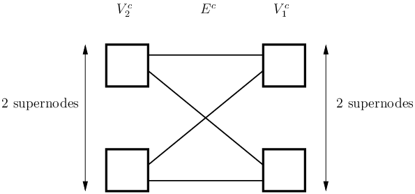
Assuming that $(n_{1}-k_{1})$ divides $n_{1}$ and $(n_{2}-k_{2})$ divides $n_{2}$ , a left check node in $\mathcal{G}^{c}$ is equivalent to $n_{2}-k_{2}$ row constraints and a right check node in $\mathcal{G}^{c}$ is equivalent to $n_{1}-k_{1}$ column constraints. An edge in the compact graph carries $(n_{1}-k_{1})\times(n_{2}-k_{2})$ code symbols. To avoid confusion between edges of $\mathcal{G}$ and $\mathcal{G}^{c}$ , we may refer to those in $\mathcal{G}^{c}$ as super-edges or equivalently as super-symbols. If $n_{i}$ is not multiple of $n_{i}-k_{i}$ , then the last row or column supernode will contain less than $n_{i}-k_{i}$ check nodes. Figure 2 depicts the compact graph of the $[4,2]^{\otimes 2}$ product code. All $[n,n/2]^{\otimes 2}$ product codes have a compact graph identical to that of $[4,2]^{\otimes 2}$ , for all $n\geq 2$ , $n$ even.

III-C Diversity and codes on graphs

From a coding point of view, diversity is the art of creating many replicas of the same information. From a channel point of view, diversity is the number of degrees of freedom available while transmitting information. In distributive storage, independent failure of individual machines is modeled by independent erasures of code symbols, while the outage of a cluster of machines is modeled as block erasures of code symbols. Assuming a storage domain with a large set of machines partitioned into $M$ clusters, diversity of distributed coding is defined as follows:

Definition 4

Consider a product code $C_{P}$ defined over $\mathbb{F}_{q}$ . Assume that symbols are given $M$ different colors. Erasing one color is equivalent to erasing all symbols having this color. The code is said to achieve a diversity $L$ if it is capable of filling all erasures after erasing $L-1$ colors. The code is full-diversity when $L=M$ .

The integer $L$ may also be called the diversity order. For Gaussian channels with fading, the diversity order appears as the slope of the error probability, i.e. $L=\lim_{\gamma\rightarrow\infty}-\frac{\log P_{e}}{\log\gamma}$ [13]. In the above definition, a cluster has been replaced by a color. We will use this terminology throughout the paper. Notice that coloring symbols is equivalent to edge coloring of the product code graph. The number of edges is $N$ in the non-compact graph and $N^{c}$ in the compact graph. In the sequel, all colorings are supposed to be perfectly balanced, i.e. $M$ divides both $N$ and $N^{c}$ and the number of edges having the same color is $N/M$ and $N^{c}/M$ for the non-compact graph and the compact graph respectively. More formally, our edge coloring is defined as follows: an edge coloring $\phi$ of $\mathcal{G}=(V_{1},V_{2},E)$ is a mapping associating one color to every edge in $E$ ,

\phi:E\rightarrow\{1,2,\ldots,M\},

(3)

such that $|\phi^{-1}(i)|=N/M$ for $i=1\ldots M$ , where $\phi^{-1}(i)$ is the inverse image of $i$ . Similarly, $\phi:E^{c}\rightarrow\{1,2,\ldots,M\}$ for $\mathcal{G}^{c}=(V^{c}_{1},V^{c}_{2},E^{c})$ and $|\phi^{-1}(i)|=N^{c}/M$ . The set of such mappings for $\mathcal{G}$ and $\mathcal{G}^{c}$ is denoted $\Phi(E)$ and $\Phi(E^{c})$ respectively.
Consider a coloring $\phi$ in $\Phi(E^{c})$ . It can be embedded into $\Phi(E)$ by copying the color of a super-edge to its associated $(n_{1}-k_{1})\times(n_{2}-k_{2})$ edges in $E$ . Thus, let $\Phi(E^{c}\rightarrow E)$ be the subset of colorings in $\Phi(E)$ obtained by embedding all colorings of $\Phi(E^{c})$ into $\Phi(E)$ . We have

\Phi(E^{c}\rightarrow E)\subset\Phi(E)\penalty\ \penalty\ \penalty\ \text{and}\penalty\ \penalty\ \penalty\ |\Phi(E^{c}\rightarrow E)|=|\Phi(E^{c})|.

(4)

The size of the edge coloring ensembles $\Phi(E)$ and $\Phi(E^{c})$ is obviously not the same when $N^{c}<N$ , which occurs for both row and column component codes not equal to single parity-check codes. Indeed, when a palette of size $M$ is used to color edges, the total number of colorings of $E$ is

|\Phi(E)|=\frac{N!}{((N/M)!)^{M}}.

(5)

This number for the compact graph is

|\Phi(E^{c})|=\frac{N^{c}!}{((N^{c}/M)!)^{M}}.

(6)

As an example, for the $[12,10]^{\otimes 2}$ code and $M=4$ , there are $2\cdot 10^{83}$ edge colorings for the non-compact graph and $2\cdot 10^{19}$ edge colorings for the compact graph. It is clear that the construction of product codes for diversity is much easier when based on $\mathcal{G}^{c}=(V^{c}_{1},V^{c}_{2},E^{c})$ because its edge coloring ensemble is smaller. Furthermore, as described below, vertices in $\mathcal{G}^{c}$ act in a way similar to standard LDPC check nodes making the design very simple. Furthermore, we will see in Section IV that edge colorings of the compact graph render larger stopping sets than colorings of the non-compact graph.

The diversity order $L$ attained by a code can never exceed $M$ , the latter being the diversity from a channel point of view. A tighter upper bound of $L$ showing the rate-diversity tradeoff is the block-fading Singleton bound. The Singleton bound for the maximal achievable diversity order is valid for all types of non-ergodic channels, including block-erasure and block-fading channels. The block-fading Singleton bound states that [31] [41]

L\leq 1+\lfloor M(1-R)\rfloor,

(7)

where $R=K/N$ is the coding rate of the product code. Codes satisfying the equality in the above Singleton bound are referred to as diversity-wise MDS or block-fading MDS codes. From (7), we deduce that $R\leq 1/M$ if $L=M$ (full-diversity coding). For example, we get $R\leq 1/2$ with an edge coloring using $L=M=2$ colors and $R\leq 1/4$ for $L=M=4$ colors. The coding rate can exceed $1/M$ when $L<M$ in applications where full diversity is not mandatory. An example suited to distributed storage is an edge coloring with a palette of $M=4$ colors, a diversity $L=2$ , and $R\leq 3/4$ .

III-D Rootcheck nodes and root symbols

In a way similar to root-LDPC codes and product codes built for block-fading channels [10][13], we introduce now the notion of root symbols and root-check nodes in product codes to be designed for distributive storage. A linear $[n,k]_{q}$ code with parity-check matrix $H$ can fill $n-k$ erasures at positions where the columns of $H$ are independent. These $n-k$ symbols correspond to $n-k$ separate edges in the non-compact graph and to a unique edge (supersymbol) in the compact graph. Therefore, for simplicity, we start by defining a root supersymbol in the compact graph where supernodes are equivalent to standard LDPC parity-check nodes.

Definition 5

Let $\mathcal{G}^{c}$ be a compact graph of a product code, let $\phi$ be a given edge coloring, and let $e\in E^{c}$ be a supersymbol. $e$ is a root supersymbol with respect to $\phi(e)$ if it admits a neighbor vertex $\upsilon$ , $\upsilon\in V^{c}_{1}$ or $\upsilon\in V^{c}_{2}$ , such that all adjacent edges $f$ in $\upsilon$ satisfy $\phi(f)\neq\phi(e)$ .

In Definition 5, if $\upsilon\in V^{c}_{1}$ then $e$ is a root supersymbol thanks to the product code column to which it belongs, i.e. $e$ can be solved in one iteration by its column component code when the color $\phi(e)$ is erased. Likewise, $e$ is protected against erasures by its row component code if $\upsilon\in V^{c}_{2}$ in the previous definition. Finally, a root supersymbol may be doubly protected by both its row and its column if both right and left neighbors $\upsilon_{1}\in V^{c}_{1}$ and $\upsilon_{2}\in V^{c}_{2}$ satisfy the condition of Definition 5.

Definition 6

Let $\mathcal{G}$ be a non-compact graph of a product code, let $\phi$ be a given edge coloring, and let $e\in E$ be a symbol. $e$ is a root symbol with respect to $\phi(e)$ if it admits a neighbor vertex $\upsilon$ such that:
$\phi(f)=\phi(e)$ for at most $n_{2}-k_{2}-1$ adjacent edges $f$ if $\upsilon\in V_{1}$ , or
$\phi(f)=\phi(e)$ for at most $n_{1}-k_{1}-1$ adjacent edges $f$ if $\upsilon\in V_{2}$ .

As mentioned in the paragraph before Definition 5, Definition 6 implies that the $n_{i}-k_{i}$ root symbols with the same color should belong to positions of independent columns in the parity-check matrix of the component code $C_{i}$ . This constraint automatically disappears for MDS component codes since any set of $n_{i}-k_{i}$ columns of $H_{i}$ has full rank.

III-E The rootcheck order in product codes

Not all symbols of a product code are root symbols. Under iterative row-column decoding on channels with block erasures, some symbols may be solved in two decoding iterations or more. Some set of symbols may never be solved and are referred to as stopping sets [17][54][51]. Our study is restricted to erasing the symbols of one color out of $M$ . Hence, the rest of this paper is restricted to double diversity, $L=2$ . Absence of diversity is equivalent to $L=1$ . We establish now the root order $\rho$ of a symbol. For root symbols satisfying definitions 5 and 6, the root order is $\rho=1$ . For symbols that can be solved after two decoding iterations, we set $\rho=2$ . The formal definition of the root order $\rho$ can be written in the following recursive manner (for $\rho\geq 2$ ).

Definition 7

Let $\mathcal{G}^{c}$ be a compact graph of a product code, let $\phi\in\Phi(E^{c})$ be an edge coloring, and let $e\in E^{c}$ be a super-symbol. $e$ has root order $\rho(e)=\min(\rho_{1},\rho_{2})$ where:
1- Let $\upsilon_{1}\in V^{c}_{1}$ be the column neighbor vertex of $e$ . $\forall f$ adjacent to $e$ in $\upsilon_{1}$ and $\phi(f)=\phi(e)$ , we have $\rho(f)<\rho_{1}$ .
2- Let $\upsilon_{2}\in V^{c}_{2}$ be the row neighbor vertex of $e$ . $\forall f$ adjacent to $e$ in $\upsilon_{2}$ and $\phi(f)=\phi(e)$ , we have $\rho(f)<\rho_{2}$ .

The previous definition implies that $\rho(e)=1$ if there exists no adjacent edge with the same color. Also, for an edge $e$ that does not admit a finite $\rho(e)$ , we set $\rho(e)=\infty$ . When color $\phi(e)$ is erased, symbols belonging to the so-called stopping sets can never be solved (even after an infinite number of decoding iterations) and hence their root order is infinite. In the next section we review stopping sets as known in the literature and we study new stopping sets for product codes based on MDS components under iterative algebraic decoding. Definition 7 can be rephrased to make it suitable for the non-compact graph $\mathcal{G}$ . We pursue this section to establish an upper bound of the largest finite root order valid for all edge colorings $\phi$ .

Theorem 1

Let $C_{P}$ be a product code $[n_{1},k_{1}]\otimes[n_{2},k_{2}]$ with a compact graph $\mathcal{G}^{c}=(V^{c}_{1},V^{c}_{2},E^{c})$ . $\forall\phi\in\Phi(E^{c})$ and $\forall e\in E^{c}$ we have:
Case 1: $\nexists f\in E^{c}$ such that $\phi(f)=\phi(e)$ and $\rho(f)=\infty$ , then

1\leq\rho(e)\leq\left\lceil\frac{N^{c}}{2M}\right\rceil=\rho_{u}.

Define the minimum number of good edges,

\eta_{min}(\phi)=\min_{i=1\ldots M}|\{f\in E^{c}:\phi(f)=i,\rho(f)=1\}|.

Then, in Case 1,

2\rho(e)+\eta_{min}(\phi)-3\leq\left\lceil\frac{N^{c}}{M}\right\rceil.

(8)

Case 2: $\exists f\in E^{c}$ such that $\phi(f)=\phi(e)$ and $\rho(f)=\infty$ , then

\rho(e)=\infty\penalty\ \penalty\ \penalty\ or\penalty\ \penalty\ \penalty\ 1\leq\rho(e)\leq\left\lceil\frac{N^{c}}{M}\right\rceil-4,

where $N^{c}=|E^{c}|$ is given by (2).

Proof:

Case 1 corresponds to a product code with diversity $L=2$ , for a given color $\phi(e)$ , which is capable of solving all symbols when that color is erased. The graph has no infinite root order symbols. $\rho$ is recursively built by starting from $\rho=1$ following two paths in the graph until reaching a common edge $e$ that has two neighboring vertices with edges of order $\rho(e)-1$ . There are up to $\lceil N^{c}/M\rceil$ edges, including $e$ , having color equal to $\phi(e)$ . The largest $\rho(e)$ is attained in the middle of the longest path of length $\lceil N^{c}/M\rceil$ , hence $2\rho(e)-1\leq\lceil N^{c}/M\rceil$ which is translated into the stated result for Case 1. An illustrated instance is given for the reader in Example 1. Back to the path of length $2\rho(e)-1$ ending with edges of order $1$ on both sides, if the population of order $1$ edges is $\eta_{1}$ for the color $\phi(e)$ , then the path can only use a maximum of $\lceil N^{c}/M\rceil-(\eta_{1}-2)$ edges. We get the inequality $2\rho(e)-1\leq\lceil N^{c}/M\rceil-(\eta_{1}-2)$ . By plugging $\eta_{min}(\phi)$ instead of $\eta_{1}$ , this inequality becomes independent from the particular color. The stated inequality in (8) is obtained after grouping $\rho(e)$ and $\eta_{min}(\phi)$ on the left side.
Case 2 corresponds to bad edge coloring where the product code does not have double diversity, i.e. stopping sets do exist for the color $\phi(e)$ . The order of $e$ may be infinite if $e$ is involved in a stopping set with another edge $f$ having the same color. Otherwise, consider the smallest stopping set of size four symbols (the smallest cycle in $\mathcal{G}^{c}$ with edges of color $\phi(e)$ ), then there remains $\lceil N^{c}/M\rceil-4$ edges of color $\phi(e)$ . A path of length $\lceil N^{c}/M\rceil-4$ starting with $\rho=1$ and ending at $\rho=\infty$ may exist. The largest finite order in this path before reaching the stopping set is $\rho=\lceil N^{c}/M\rceil-4$ . ∎

Corollary 1

Let $C_{P}$ be a product code $[n_{1},k_{1}]\otimes[n_{2},k_{2}]$ with a compact graph $\mathcal{G}^{c}$ . Let $\phi\in\Phi(E^{c})$ be an edge coloring. We define

\rho_{max}(\phi)=\max_{e\in E^{c}}\rho(e).

(9)

$C_{P}$ attains double diversity under iterative row-column decoding if and only if $\rho_{max}(\phi)<\infty$ . In this case, we say that $\phi$ is a double-diversity coloring and $\forall e\in E^{c}$ , $e$ can be solved after at most $\rho_{max}$ decoding iterations where $\rho_{max}(\phi)\leq\rho_{u}$ .

For colorings in $\Phi(E)$ , we extend the same definition as in Corollary 1 and we say that $\phi\in\Phi(E)$ is double-diversity if all edges have a finite rootcheck order. The parameter $\rho_{max}$ is important in practical applications to bound from above the amount of conveyed information within a network (whether it is a local-area or a wide-area network). In fact, in coding for distributed storage, the locality of a product code per decoding iteration is $\max(n_{1},n_{2})$ in $\mathcal{G}$ under algebraic decoding of its row and column components. Here, the locality is the number of symbols to be accessed in order to repair an erased symbol [25]. Locality is $\max(k_{1},k_{2})$ for MDS components under ML decoding of the product code components. Finally, for a product code, the information transfer per symbol is bounded from above by

\rho_{max}(\phi)\times\max(n_{1},n_{2}).

(10)

The exact transfer cost to fill all erasures with iterative decoding can be determined by multiplying each order $\rho$ with the corresponding edge population size. This exact cost may vary in a wide range from one coloring to another. The DECA algorithm presented in Section V dramatically reduces $\rho_{max}$ by enlarging the edge population with root order $1$ . The interdependence between $\rho$ and the population of order $1$ was revealed in inequality (8). This inequality is useful in intermediate cases where $\rho_{max}=1$ is not attained, i.e. outside the case where all edges have order $1$ . The influence of the component decoding method on the performance of a product code via its stopping sets is discussed in Section IV.

Example 1

Consider a $[12,10]^{\otimes 2}$ product code and a coloring $\phi$ with $M=4$ colors. The compact graph has $|E^{c}|=6\times 6$ edges. Instead of drawing $\mathcal{G}^{c}$ , we draw the $6\times 6$ compact matrix representation of the product code in Fig. 3. Supersymbols corresponding to a color $\phi(e)=1$ are shaded. Fig. 3 also shows a path in $\mathcal{G}^{c}$ such that a maximal order $\rho_{max}=\rho_{u}=5$ is attained for $\phi(e)=1$ . If $\phi$ has double diversity then $\rho_{max}$ will not exceed $\rho_{u}=5$ for all colors $\phi(e)\in\{1,2,\ldots,M\}$ . Note that the parameters of this product code are such that $N^{c}/M-4$ is also equal to 5 for a $\phi$ with a diversity defect.

Example 2

Consider a $[14,12]\otimes[16,14]$ product code and a coloring $\phi$ with $M=4$ colors. The compact graph has $|E^{c}|=7\times 8$ edges. The compact matrix and a path attaining $\rho=10$ are illustrated in Fig. 4. $\phi$ is chosen such that the first color has a cycle involving four supersymbols. Starting from the root supersymbol ( $\rho=1$ ) it is possible to create a path in the graph such that $\rho=10$ is reached. Note that a double-diversity $\phi$ cannot exceed a root order $\rho_{u}=7$ .

The ideal situation is to construct a product code and its edge coloring in order to obtain $\rho(e)=1$ for all edges. We investigate now the conditions on the product code rate and its components rates in this ideal situation. The analysis based on $\rho_{u}$ reveals the existence of a trade-off between minimizing the number of decoding iterations and the valid range of both coding rates for the product code components.

Firstly, let us look at the upper bound $\rho_{u}$ from Theorem 1. Without loss of generality, assume that $n_{i}-k_{i}$ divides $n_{i}$ . Then, we have

R_{i}=1-\frac{n_{i}-k_{i}}{n_{i}}=1-\frac{1}{|V^{c}_{i}|}.

(11)

The total coding rate becomes

R=R_{1}R_{2}=\left(1-\frac{1}{|V^{c}_{1}|}\right)\cdot\left(1-\frac{1}{|V^{c}_{2}|}\right).

(12)

Using $N^{c}=|V^{c}_{1}|\cdot|V^{c}_{2}|$ , we get

R_{1}R_{2}=R_{1}+R_{2}-1+\frac{1}{N^{c}}.

(13)

Finally, from (13) and Theorem 1, the upper bound of the root order for double-diversity edge coloring of the compact graph can be expressed as

\rho_{u}=\left\lceil\frac{N^{c}}{2M}\right\rceil=\left\lceil\frac{1}{2M\times(1+R_{1}R_{2}-R_{1}-R_{2})}\right\rceil.

(14)

Fix the product code rate $R$ , force the upper bound to $\rho_{u}=1$ , and take $M=4$ colors. Then the denominator in (14) should be less than $1$ or equivalently $-8R_{1}^{2}+(7+8R)R_{1}-8R\penalty\ >\penalty\ 0$ . This second-degree polynomial in $R_{1}$ is non-negative if and only if

R<\frac{9}{8}-\frac{1}{\sqrt{2}}\approx 0.4178,

(15)

and

-\sqrt{64R^{2}-144R+49}<16R_{1}-8R-7<+\sqrt{64R^{2}-144R+49}.

(16)

As a result, with a palette of four colors, (15) tells us that $\rho(e)=1$ for all edges is feasible for a product code with a rate less than $0.4178$ . It is obvious that (15) is a very constraining condition because $\rho_{u}$ is an upper bound of $\rho_{max}(\phi)$ for all $\phi\in\Phi(E^{c})$ . It is worth noting that $R_{1}$ and $R_{2}$ vary in a smaller range when $R$ approaches $\frac{9}{8}-\frac{1}{\sqrt{2}}$ , which corresponds to a product code with balanced components.

In Section V-A, we will show unbalanced product codes where a sufficient condition on the component rates imposes order $1$ to all edges. The sufficient condition, not based on $\rho_{u}$ , is given by Lemma 5. But before introducing an efficient edge coloring algorithm in Section V, we analyze stopping sets in product codes with MDS components in the next section, we describe the relationship between stopping sets and the product code graph representation, and finally we enumerate obvious and non-obvious stopping sets. Stopping sets enumeration is useful to determine the performance of a product code with and without edge coloring.

IV Stopping sets for MDS components

The purpose of this section is to prepare the way for determining the performance of iterative decoding of non-binary product codes. The analysis of stopping sets in a product code will yield a tight upper bound of its iterative decoding performance over a channel with independent erasures. The same analysis will be useful to accurately estimate the performance under edge coloring in presence of block and multiple erasure channels.

IV-A Decoding erasures

Definition 8

An erasure pattern is said to be ML-correctable if the ML decoder is capable of solving all its erased symbols.

For an erasure pattern which is not correctable under ML or iterative decoding, the decoding process may fill none or some of the erasures and then stay stuck on the remaining ones. Before describing the stopping sets of a product code, let us recall some fundamental results regarding the decoding of its row and column component codes. The ML erasure-filling capability of a linear code satisfies the following property.

Proposition 1

Let $C[n,k,d]_{q}$ be a linear code with $q\geq 2$ . Assume that $C$ is not MDS and the $n$ symbols of a codeword are transmitted on an erasure channel. Then, there exists an erasure pattern of weight greater than $d-1$ that is ML-correctable.

Proof:

Let $H$ be an $(n-k)\times n$ parity-check matrix of $C$ with rank $n-k>d-1$ . For any integer $w$ in the range $[d,n-k]$ , there exists a set of $w$ linearly independent columns in $H$ . Choose an erasure pattern of weight $w$ with erasures located at the positions of the $w$ independent columns. Then, the ML decoder is capable of solving all these erasures by simple Gaussian reduction of $H$ . ∎For MDS codes, based on a proof similar to the proof of Proposition 1, we state a well-known result in the following corollary.

Corollary 2

Let $C[n,k,d]_{q}$ be an MDS code. All erasure patterns of weight greater than $d-1$ are not ML-correctable.

We conclude from the previous corollary that an algebraic decoder for an MDS code attains the word-error performance of its ML decoder. What about symbol-error performance? Indeed, for general binary and non-binary codes, the ML decoder may outperform an algebraic decoder since it is capable of filling some of the erasures when dealing with a pattern which is not ML-correctable. In the MDS case, the answer comes from the absence of spectral holes for any MDS code beyond its minimum distance. This basic result is proven via standard tools from algebraic coding theory [40][7]:

Proposition 2

Let $C[n,k,d]_{q}$ be a non-binary MDS code ( $q>n>2$ ). For any $w$ satisfying $d\leq w\leq n$ and any support $\mathcal{X}=\{i_{1},i_{2},\ldots,i_{w}\}$ , where $1\leq i_{j}\leq n$ , there exists a codeword in $C$ of weight $w$ having $\mathcal{X}$ as its own support.

Proof:

By assumption we have $w>r=n-k$ . Let $H$ be a parity-check matrix of $C$ with rank $r=n-k$ . Recall that the MDS property makes full-rank any set of $n-k$ columns of $H$ [40]. $w$ is written as $w=r+\ell$ , where $\ell=1\ldots k$ . The $w$ positions of $\mathcal{X}$ are anywhere inside the range $[1,n]$ , but for simplicity let us denote $h_{1}\ldots h_{r}$ the $r$ columns of $H$ in the first $r$ positions. The last $\ell$ columns are denoted $\zeta_{1}\ldots\zeta_{\ell}$ . For any $j=1\ldots\ell$ , we have

\zeta_{j}=\sum_{i=1}^{r}a_{i,j}h_{i},

where $a_{i,j}\in\mathbb{F}_{q}\setminus\{0\}$ otherwise it contradicts $d=n-k+1$ . Now, select $\alpha_{1}\ldots\alpha_{\ell}$ from $\mathbb{F}_{q}\setminus\{0\}$ such that: $\alpha_{1}$ is arbitrary, $\alpha_{2}$ is chosen outside the set $\{-\alpha_{1}a_{i,1}/a_{i,2}\}_{i=1}^{r}$ , then $\alpha_{3}$ is chosen outside the set $\{(-\alpha_{1}a_{i,1}-\alpha_{2}a_{i,2})/a_{i,3}\}_{i=1}^{r}$ , and so on, up to $\alpha_{\ell}$ which is chosen outside the set $\{-\sum_{u=1}^{\ell-1}\alpha_{u}a_{i,u}/a_{i,\ell}\}_{i=1}^{r}$ . Here, the notation $a/b$ in $\mathbb{F}_{q}\setminus\{0\}$ is equivalent to the standard algebraic notation $ab^{-1}$ . The equality

\sum_{j=1}^{\ell}\alpha_{j}\zeta_{j}=\sum_{i=1}^{r}\sum_{j=1}^{\ell}\alpha_{j}a_{i,j}h_{i}

produces a codeword of Hamming weight $w$ . Hence, there exists a codeword of weight $w$ with non-zero symbols in all positions given by $\mathcal{X}$ . ∎Now, at the symbol level for an MDS code and an erasure pattern which is not ML-correctable ( $w>d-1$ ), we conclude from Proposition 2 that the ML decoder cannot solve any of the $w$ erasures because they are covered by a codeword. Consequently, an algebraic decoder for an MDS code also attains the symbol-error performance of the ML decoder. This behavior will have a direct consequence on the iterative decoding of a product code with MDS components: stopping sets are identical when dealing with algebraic and ML-per-component decoders.

A general description of a stopping set was given by Definition 1. The exact definition of a stopping set depends on the iterative decoding type. For product codes, four decoding methods are known:

•

Type I: ML decoder. This is a non-iterative decoder. It is based on a Gaussian reduction of the parity-check matrix of the product code.
•

Type II: Iterative algebraic decoder. At odd decoding iterations, component codes $C_{1}$ on each column are decoded via an algebraic decoder (bounded-distance) that fills up to $d-1$ erasures. Similarly, at even decoding iterations, component codes $C_{2}$ on each row are decoded via an algebraic decoder.
•

Type III: Iterative ML-per-component decoder. This decoder was considered by Rosnes in [51] for binary product codes. At odd decoding iterations, column codes $C_{1}$ are decoded via an optimal decoder (ML for $C_{1}$ ). At even decoding iterations, row codes $C_{2}$ are decoded via a similar optimal decoder (ML for $C_{2}$ ).
•

Type IV: Iterative belief-propagation decoder based on the Tanner graph of $C_{\mathcal{P}}$ , as studied by Schwartz et al. for general linear block codes [54] and by Di et al. for low-density parity-check codes [17].

The three iterative decoders listed above give rise to three different kinds of stopping sets. As previously indicated, from Corollary 2 and Propositions 2, we concluded that type-II and type-III stopping sets are identical if component codes are MDS.

IV-B Stopping set definition

Let $C$ be a $q$ -ary linear code of length $n$ , i.e. $C$ is a sub-space of dimension $k$ of $\mathbb{F}_{q}^{n}$ . The support of $C$ , denoted by $\mathcal{X}(C)$ , is the set of $\ell$ distinct positions $\{i_{1},i_{2},\ldots,i_{\ell}\}=\{i_{j}\}_{j=1}^{\ell}$ , $1\penalty\ \leq\penalty\ i_{j}\penalty\ \leq\penalty\ n$ , such that, for all $j$ , there exists a codeword $c=(c_{1}\ldots c_{n})\in C$ with $c_{i_{j}}\neq 0$ . This notion of support $\mathcal{X}$ is applied to rows and columns in a product code.

Now, we define a rectangular support which is useful to represent a stopping set in a bi-dimensional product code. Let $\mathcal{S}\subseteq\{1,\ldots,n_{1}\}\times\{1,\ldots,n_{2}\}$ be a set of symbol positions in the product code. The set of row positions associated to $\mathcal{S}$ is $\mathcal{R}_{1}(\mathcal{S})=\{i_{1},\ldots,i_{\ell_{1}}\}$ where $|\mathcal{R}_{1}(\mathcal{S})|=\ell_{1}$ and for all $i\in\mathcal{R}_{1}(\mathcal{S})$ there exists $(i,\ell)\in\mathcal{S}$ . The set of column positions associated to $\mathcal{S}$ is $\mathcal{R}_{2}(\mathcal{S})=\{j_{1},\ldots,j_{\ell_{2}}\}$ where $|\mathcal{R}_{2}(\mathcal{S})|=\ell_{2}$ and for all $j\in\mathcal{R}_{2}(\mathcal{S})$ there exists $(\ell,j)\in\mathcal{S}$ . The rectangular support of $\mathcal{S}$ is

\mathcal{R}(\mathcal{S})=\mathcal{R}_{1}(\mathcal{S})\times\mathcal{R}_{2}(\mathcal{S}),

(17)

i.e. the smallest $\ell_{1}\times\ell_{2}$ rectangle including all columns and all rows of $\mathcal{S}$ .

Definition 9

Consider a product code $C_{P}=C_{1}\otimes C_{2}$ . Let $\mathcal{S}\subseteq\{1,\ldots,n_{1}\}\times\{1,\ldots,n_{2}\}$ with $|\mathcal{R}_{1}(\mathcal{S})|=\ell_{1}$ and $|\mathcal{R}_{2}(\mathcal{S})|=\ell_{2}$ . Consider the $\ell_{1}$ rows of $\mathcal{S}$ given by $\mathcal{S}_{r}^{(i)}=\{j:(i,j)\in\mathcal{S}\}$ and the $\ell_{2}$ columns of $\mathcal{S}$ given by $\mathcal{S}_{c}^{(j)}=\{i:(i,j)\in\mathcal{S}\}$ . The set $\mathcal{S}$ is a stopping set of type III for $C_{P}$ if there exist linear subcodes $C_{c}^{(j)}\subseteq C_{1}$ and $C_{r}^{(i)}\subseteq C_{2}$ such that $\mathcal{X}(C_{c}^{(j)})=\mathcal{S}_{c}^{(j)}$ and $\mathcal{X}(C_{r}^{(i)})=\mathcal{S}_{r}^{(i)}$ for all $i\in\mathcal{R}_{1}(\mathcal{S})$ and for all $j\in\mathcal{R}_{2}(\mathcal{S})$ .

The cardinality $|\mathcal{S}|$ is called the size of the stopping set and will also be referred to in the sequel as the weight of $\mathcal{S}$ . Recall that type II and type III stopping sets are identical when both $C_{1}$ and $C_{2}$ are MDS. Stopping sets of type III were studied for binary product codes by Rosnes [51]. His analysis is based on the generalized Hamming distance [67][29] because sub-codes involved in Definition 9 may have a dimension greater than 1. In the non-binary MDS case, according to Proposition 2, all these sub-codes have dimension 1, i.e. they are generated by a single non-zero codeword. Consequently, the generalized Hamming distance is not relevant when using MDS components. In such a case, the analysis of type II stopping sets is mainly combinatorial and does not require algebraic tools.

Stopping sets for decoder types II-IV can be characterized by four main properties summarized as follows.

•

Obvious or not obvious sets, also known as rank-1 sets. A stopping set $\mathcal{S}$ is obvious if $\mathcal{S}=\mathcal{R}(\mathcal{S})$ .
•

Primitive or non-primitive stopping sets. A stopping set is primitive if it cannot be partitioned into two or more smaller stopping sets. Notice that all stopping sets, whether they are primitive or not, are involved in the code performance.
•

Codeword or non-codeword. A stopping set $\mathcal{S}$ is said to be a codeword stopping set if there exists a codeword $c$ in $C_{P}$ such that $\mathcal{X}(c)=\mathcal{S}$ .
•

ML-correctable or non-ML-correctable. A stopping set $\mathcal{S}$ cannot be corrected via ML decoding if it includes the support of a non-zero codeword.

In the remaining material of this paper, we restrict our study to type II stopping sets.

Example 3

Consider a $[n_{1},n_{1}-2,3]_{q}\otimes[n_{2},n_{2}-2,3]_{q}$ product code. A stopping set $\mathcal{S}$ of size $w=9$ is shown as a weight- $9$ matrix of size $n_{1}\times n_{2}$ , where $1$ corresponds to an erased position:

\mathcal{S}\penalty\ =\penalty\ \left(\begin{array}[]{ccccccc}0&0&0&0&0&0\\ 0&0&0&0&0&0\\ 0&1&0&1&1&0\\ 0&0&0&0&0&0\\ 0&1&0&1&1&0\\ 0&1&0&1&1&0\\ 0&0&0&0&0&0\end{array}\right).

(18)

We took $n_{1}=n_{2}=7$ for illustration. The rectangular support is shown in a compact representation as a matrix of size $\ell_{1}\times\ell_{2}=3\times 3$ ,

\mathcal{R}(\mathcal{S})\penalty\ =\penalty\ \left(\begin{array}[]{ccc}1&1&1\\ 1&1&1\\ 1&1&1\end{array}\right).

(19)

The stopping set in (18) is obvious, it has the same size as its rectangular support. It corresponds to a matrix of rank 1. Each row and each column of $\mathcal{S}$ has weight $3$ . Iterative row-column decoding based on component algebraic decoders fails in decoding rows and columns since the number of erasures exceeds the erasure-filling capacity of the MDS components. This stopping set is not ML-correctable because it is a product-code codeword. In the sequel, all stopping sets (type II) shall be represented in this compact manner by a smaller rectangle of size $\ell_{1}\times\ell_{2}$ .

Example 4

For the same $[n_{1},n_{1}-2,3]_{q}\otimes[n_{2},n_{2}-2,3]_{q}$ product code used in the previous example, the following stopping sets of size $12$ are not obvious.

\mathcal{S}_{1}\penalty\ =\penalty\ \left(\begin{array}[]{ccccccc}0&0&0&0&0&0&0\\ 0&0&0&0&0&0&0\\ 0&1&1&1&0&0&0\\ 0&0&1&1&1&0&0\\ 0&1&0&1&1&0&0\\ 0&1&1&0&1&0&0\\ 0&0&0&0&0&0&0\end{array}\right),

(20)

\mathcal{S}_{2}\penalty\ =\penalty\ \left(\begin{array}[]{ccccccc}0&0&0&0&0&0&0\\ 0&0&0&0&0&0&0\\ 0&1&0&1&1&0&0\\ 0&0&0&1&1&1&0\\ 0&1&0&0&1&1&0\\ 0&1&0&1&0&1&0\\ 0&0&0&0&0&0&0\end{array}\right).

(21)

In compact form, their rectangular support is

\mathcal{R}(\mathcal{S}_{1})\penalty\ =\penalty\ \mathcal{R}(\mathcal{S}_{2})\penalty\ =\penalty\ \left(\begin{array}[]{cccc}1&1&1&0\\ 0&1&1&1\\ 1&0&1&1\\ 1&1&0&1\end{array}\right).

(22)

These stopping sets have size $12$ and a $4\times 4$ rectangular support. For $w=12$ , it is also possible to build an obvious stopping set in a $3\times 4$ rectangle or a $4\times 3$ rectangle full of $1$ . $\mathcal{S}_{1}$ is ML-correctable since it does not cover a product code codeword. $\mathcal{S}_{2}$ covers a codeword hence it is not ML-correctable.

IV-C Stopping sets and subgraphs of product codes

A stopping set as defined by Definition (9) corresponds to erased edges in the non-compact graph $\mathcal{G}$ introduced in Section III-A. Indeed, consider the size- $9$ stopping set given by (18) or (19). The nine symbol positions involve nine edges in $\mathcal{G}$ , three row checknodes, and three column checknodes. Each of these six checknodes has three erased symbols making the $[12,10,3]$ decoder fail. This stopping set is equivalent to a subgraph of $9$ edges in $\mathcal{G}$ as shown in Figure 5.

The subgraph in Figure 5 has three length- $4$ cycles and two length- $6$ cycles. The small cycles of length- $4$ are associated to an erasure pattern with a $2\times 2$ rectangular support which is not a stopping set ( $d_{1}=d_{2}=3$ ). Similarly, length- $6$ cycles are not stopping sets and are associated to erasure patterns with a $2\times 3$ rectangular support. We will see in the next section that the minimum stopping set size is $d_{1}d_{2}=9$ , i.e. it is equal to the minimum Hamming distance of the product code.

A subgraph of $\mathcal{G}^{c}$ can be embedded into $\mathcal{G}$ by splitting each super-edge into $(n_{1}-k_{1})\times(n_{2}-k1)$ edges. The converse is not always true. The subgraph with nine edges in Figure 5 cannot be compressed into a subgraph of $\mathcal{G}^{c}$ . For the $[12,10,3]^{\otimes 2}$ product code, a supersymbol in $\mathcal{G}^{c}$ contains four edges. Hence, a necessary condition for a stopping set in $\mathcal{G}$ to become a valid stopping set in $\mathcal{G}^{c}$ is to erase edges in groups of $4$ . Knowing that type II and type III stopping sets are identical when row and column codes $C_{1}$ and $C_{2}$ are MDS, Definition (9) leads to the following corollaries.

Corollary 3

Let $C_{P}=C_{1}\otimes C_{2}$ be a product code with MDS components $C_{1}$ and $C_{2}$ having minimum Hamming distance $d_{1}$ and $d_{2}$ respectively. Assume that symbols (edges) of $\mathcal{G}=(V_{1},V_{2},E)$ are sent over an erasure channel. A stopping set for the iterative decoder is a subgraph of $\mathcal{G}$ such that all column vertices in $V_{1}$ have a degree greater than or equal to $d_{1}$ and all row vertices in $V_{2}$ have a degree greater than or equal to $d_{2}$ .

Corollary 4

Let $C_{P}=C_{1}\otimes C_{2}$ be a product code with MDS components $C_{1}$ and $C_{2}$ having minimum Hamming distance $d_{1}$ and $d_{2}$ respectively. Assume that supersymbols (super-edges) of $\mathcal{G}^{c}=(V^{c}_{1},V^{c}_{2},E^{c})$ are sent over an erasure channel. A stopping set for the iterative decoder is a subgraph of $\mathcal{G}^{c}$ such that all column vertices in $V^{c}_{1}$ have a degree greater than or equal to $2$ and all row vertices in $V_{2}$ have a degree greater than or equal to $2$ .

The above corollaries suppose a symbol (or a supersymbol) channel with independent erasures. When $\mathcal{G}$ is endowed with an edge coloring $\phi$ , we get the same constraint on the validity of a subgraph embedding from $\mathcal{G}^{c}$ into $\mathcal{G}$ . We know from Section III-A that $\Phi(E^{c}\rightarrow E)$ is a subset of $\Phi(E)$ , i.e. some edge colorings of $\mathcal{G}$ are not edge colorings of $\mathcal{G}^{c}$ . Consequently, on a block-erasure channel, if all super-edges of the same color are erased, stopping sets in $\mathcal{G}^{c}$ are a subset of those in $\mathcal{G}$ . The non-compact graph $\mathcal{G}$ has a larger ensemble of stopping sets, with or without edge coloring. As an example, for the $[12,10,3]^{\otimes 2}$ product code, the smallest stopping set in $\mathcal{G}^{c}$ has size $2\times 2$ when four super-edges are erased which yields a stopping set of size $16$ in $\mathcal{G}$ .

Example 5

Consider the $[9,6,4]_{q}^{\otimes 2}$ product code where $d_{1}=d_{2}=4$ and $q>9$ . Assume that our palette has $M=3$ colors. The non-compact graph admits an ensemble of $|\Phi(E)|\penalty\ =\penalty\ 4490186382903298862950669893074864640$ edge colorings! The compact graph has $|\Phi(E^{c})|\penalty\ =\penalty\ 1680$ only. In $\mathcal{G}^{c}$ , each color is used $N^{c}/M=3$ times. For a channel erasing all symbols of the same color, the compact graph has no stopping sets (the $2\times 2$ rectangular support cannot be filled by a single color). A compact matrix representation of $\mathcal{G}^{c}$ attaining double diversity with all symbols of order 1 is given by the trivial matrix

\left[\begin{array}[]{ccc}R&G&B\\ B&R&G\\ G&B&R\end{array}\right],

(23)

where the color $\phi(e)=1$ is replaced by the letter ’R’, $\phi(e)=2$ is replaced by the letter ’G’, and $\phi(e)=3$ is replaced by the letter ’B’. The non-compact graph has $9\times 9$ edges, each color is used $27$ times. Double diversity is lost in $\mathcal{G}$ if one of the $4\times 4$ , $4\times 5$ , or $5\times 5$ obvious stopping sets is covered by a unique color. Clearly, $\mathcal{G}^{c}$ makes the design much easier. This double-diversity product code has a relatively low coding rate. More challenging product code designs are given in Section V with higher rates up to the one imposed by the block-fading/block-erasure Singleton bound.

IV-D Enumeration of stopping sets

For a fixed non-zero integer $w$ , the number of stopping sets of size $w$ , denoted as $\tau_{w}$ , falls in two different cases. Firstly, $\tau_{w}\penalty\ =\penalty\ 0$ if $w$ is small with respect to the minimum Hamming distance of the product code. Also, $\tau_{w}=0$ for special erasure patterns obtained by adding a small neighborhood to a smaller obvious set. Secondly, for both obvious and non-obvious stopping sets, $\tau_{w}$ is non-zero and the weight $w$ may correspond to many rectangular supports of different height and width. The code performance over erasure channels is dominated by not-so-large stopping sets. Non-empty stopping sets of the second case satisfy the general property stated in the following lemma.

Lemma 1

Given a weight $w\leq(d_{1}+1)(d_{2}+1)$ and assuming $\tau_{w}>0$ , then $\exists\mathcal{S}^{0}$ such that $\forall\mathcal{S}$ with $|\mathcal{S}|=w$ , we have $\|\mathcal{R}(\mathcal{S})\|\leq\|\mathcal{R}(\mathcal{S}^{0})\|=(\ell_{1}^{0},\ell_{2}^{0})$ , where

	$\displaystyle\ell_{1}^{0}$	$\displaystyle\leq d_{1}+1+\left\lfloor\frac{d_{1}+1}{d_{2}}\right\rfloor,$		(24)
	$\displaystyle\ell_{2}^{0}$	$\displaystyle\leq d_{2}+1+\left\lfloor\frac{d_{2}+1}{d_{1}}\right\rfloor.$		(25)

Proof:

Let $w$ be equal to $(d_{1}+1)(d_{2}+1)$ . In order to establish an upper bound of the height $\ell_{1}$ , we build the highest possible rectangular support for this weight $w$ . Assume the rectangle is $\ell_{1}^{0}\times\ell_{2}$ , each of its rows should have at least $d_{2}$ erasures to make the type-II decoder fail. Then $d_{2}\ell_{1}^{0}\leq(d_{1}+1)(d_{2}+1)$ which becomes the upper bound given by (24). Now, if $w$ is less than $(d_{1}+1)(d_{2}+1)$ , the rectangular support of the stopping set can only shrink in size. The upper bound of the width in (25) is proven in a similar way. ∎The above lemma states the existence of a maximal rectangular support for a given stopping set size. The example given below cites stopping sets with a unique-size rectangular support and stopping sets with multiple-size rectangular supports.

Example 6

Consider a $C_{1}\otimes C_{2}$ product code where $C_{1}$ and $C_{2}$ are both MDS with minimum Hamming distance $3$ . The stopping set given by (19) cannot have a large rectangular support. In general, all stopping sets of size $d_{1}d_{2}$ have a rectangular support of fixed dimensions $d_{1}\times d_{2}$ . Now, let $w=12$ . As indicated in Example 4, stopping sets of size $12$ may be included in rectangular supports of dimensions $3\times 4$ , $4\times 3$ , and $4\times 4$ . For $w=12$ , it is impossible to build a $4\times 5$ rectangular support (reductio ad absurdum) making $\ell_{1}^{0}=4$ and $\ell_{2}^{0}=4$ . A similar proof by contradiction yields $\ell_{1}^{0}=5$ and $\ell_{2}^{0}=5$ for $w=15$ .

The next lemma gives an obvious upper bound of the size of $\mathcal{R}(\mathcal{S})$ by stating a simple limit on the number of zeros (non-erased positions) inside $\mathcal{R}(\mathcal{S})$ .

Lemma 2

Let $\mathcal{R}(\mathcal{S})$ be the $\ell_{1}\times\ell_{2}$ rectangular support of a stopping set $\mathcal{S}$ of size $w$ . Let $\beta=\ell_{1}\ell_{2}-w$ be the number of zero positions, or equivalently $\beta$ is the size of the set $\mathcal{R}(\mathcal{S})\setminus\mathcal{S}$ . Then

\beta\leq\min((\ell_{1}-d_{1})\ell_{2},\ell_{1}(\ell_{2}-d_{2})).

(26)

Before stating and proving Theorem 2, we announce two results in Lemma 3 and Lemma 4 on bipartite graphs enumeration. We saw in the previous section that stopping sets are sub-graphs of $\mathcal{G}$ and $\mathcal{G}^{c}$ , see Corollary 3 and Corollary 4. In other words, the enumeration of stopping sets represented as matrices of a given distribution of row weight and column weight is equivalent to enumerating bipartite graphs where left vertices stand for rows and right vertices stand for columns. An edge should be drawn between a left vertex and a right vertex according to some rule, e.g. the rule used in the previous section draws an edge in the bipartite graph for each $1$ in the stopping set matrix. Stopping sets enumeration in the next theorem is based on $\beta$ , the number of zeros or the number of non-erased positions. Hence, we shall use the opposite rule. A stopping set of weight $w$ and having a $\ell_{1}\times\ell_{2}$ rectangular support shall be represented by a bipartite graph with $\ell_{1}$ left vertices, $\ell_{2}$ right vertices, and a total of $\beta=\ell_{1}\ell_{2}-w$ edges. Notice that these bipartite graphs have no length-2 cycles because parallel edges are forbidden.

For finite $\ell_{1}$ and $\ell_{2}$ , given the left degree distribution and the right degree distribution, there exists no exact formula for counting bipartite graphs. The best recent results are asymptotic in the graph size for sparse and dense matrices [14] [16] and cannot be applied in our enumeration. The following two lemmas solve two cases encountered in Theorem 2 for $w=d(d+2)$ and $w=(d+1)(d+1)$ both inside a $(d+2)\times(d+2)$ rectangular support. The definition of special partitions is required before introducing the two lemmas.

Definition 10

Let $\ell\geq 2$ be an integer. A special partition of length $j$ of $\ell$ is a partition defined by a tuple $(\ell_{1},\ell_{2},\ldots,\ell_{j})$ such that its integer components satisfy:

•

$\ell_{1}\leq\ell_{2}\leq\ldots\leq\ell_{j}$ .
•

$\sum_{i=1}^{j}\ell_{i}=\ell$ .
•

$\ell_{i}\geq 2$ , $\forall j$ .
•

$1\leq j\leq\ell/2$ .

A special partition shall be denoted by $((\ell_{1},\ldots,\ell_{j}))$ .

Definition 11

The group number of a special partition, denoted by $\kappa=\kappa(\ell_{1},\ell_{2},\ldots,\ell_{j})$ , is the number of different integers $\ell_{j}$ , for $j=1\ldots\ell/2$ . In other words, following set theory, the set including the $j$ integers $\ell_{i}$ ’s is $\{\ell_{i_{1}},\ell_{i_{2}},\ldots,\ell_{i_{\kappa}}\}$ . The group number divides the partition of $\ell$ into $\kappa$ groups where the $m^{th}$ group includes $\ell_{i_{m}}$ repeated $g_{m}$ times, and $\sum_{m=1}^{\kappa}g_{m}=j$ .

Lemma 3

Consider bipartite graphs defined as follows: $\ell$ left vertices, $\ell$ right vertices, all vertices have degree 2, and no length-2 cycles are allowed. For $\ell\geq 2$ , the total number $x_{\ell}$ of such bipartite graphs is given by the expression

x_{\ell}=\sum_{((\ell_{1},\ldots,\ell_{j}))}\frac{1}{\prod_{m=1}^{\kappa(\ell_{1},\ldots,\ell_{j})}g_{m}!}\prod_{k=1}^{j}\frac{\prod_{u=0}^{\ell_{k}-1}(\ell-\sum_{i=1}^{k-1}\ell_{i}-u)^{2}}{2\ell_{k}}

(27)

where $\sum_{((\ell_{1},\ldots,\ell_{j}))}$ is a summation over all special partitions of the integer $\ell$ , $\kappa(\ell_{1},\ldots,\ell_{j})$ is the group number of the special partition $((\ell_{1},\ldots,\ell_{j}))$ , and $g_{m}$ is the size of the $m^{th}$ group.

Proof:

Firstly, let us find the number of Hamiltonian bipartite graphs having $\ell_{k}$ left vertices, $\ell_{k}$ right vertices, all vertices of degree $2$ , and no length- $2$ cycles allowed. There are $(\ell_{k}!)^{2}$ ways to choose the order of all left and right vertices. If the Hamiltonian cycle is represented by a sequence of $2\ell_{k}$ integers corresponding to the $2\ell_{k}$ vertices of the bipartite graph, then there are $2\ell_{k}$ ways to shift the Hamiltonian cycle without changing the graph. Hence, the number of Hamiltonian bipartite graphs of degree $2$ is

\frac{(\ell_{k}!)^{2}}{2\ell_{k}}.

(28)

Secondly, given the half-size $\ell$ of the bipartite graph stated in this lemma, all special partitions of $\ell$ are considered. For a fixed special partition $((\ell_{1},\ell_{2},\ldots,\ell_{j}))$ the bipartite graph is decomposed into $j$ Hamiltonian graphs each of length $\ell_{k}$ , $k=1\ldots j$ . The number of choices for selecting the vertices of the $j$ Hamiltonian graphs is

\prod_{k=1}^{j}{\ell-\sum_{i=1}^{k-1}\ell_{i}\choose\ell_{k}}^{2}.

(29)

The above number should be multiplied by the number of Hamiltonian graphs for each selection of vertices to get

\prod_{k=1}^{j}{\ell-\sum_{i=1}^{k-1}\ell_{i}\choose\ell_{k}}^{2}\frac{\left(\ell_{k}!\right)^{2}}{2\ell_{k}}.

(30)

But for a given special partition, each group of size $g_{m}$ is creating $g_{m}!$ identical bipartite graphs. Hence, the final result for a fixed partition becomes

\frac{1}{\prod_{m=1}^{\kappa(\ell_{1},\ldots,\ell_{j})}g_{m}!}\prod_{k=1}^{j}{\ell-\sum_{i=1}^{k-1}\ell_{i}\choose\ell_{k}}^{2}\frac{\left(\ell_{k}!\right)^{2}}{2\ell_{k}}.

(31)

Then, $x_{\ell}$ is obtained by summing (31) over all special partitions of the integer $\ell$ to yield

x_{\ell}=\sum_{((\ell_{1},\ldots,\ell_{j}))}\frac{1}{\prod_{m=1}^{\kappa(\ell_{1},\ldots,\ell_{j})}g_{m}!}\prod_{k=1}^{j}{\ell-\sum_{i=1}^{k-1}\ell_{i}\choose\ell_{k}}^{2}\frac{\left(\ell_{k}!\right)^{2}}{2\ell_{k}}.

(32)

The simplification of the factors $(\ell_{k}!)^{2}$ yields the expression stated by this lemma. ∎

Lemma 4

Consider bipartite graphs defined as follows: $\ell$ left vertices, $\ell$ right vertices, all left vertices have degree $2$ except one vertex of degree $1$ , all right vertices have degree $2$ except one vertex of degree $1$ , and finally no length- $2$ cycles are allowed. For $\ell\geq 3$ , the total number $y_{\ell}$ of such bipartite graphs is

y_{\ell}=\ell^{2}\cdot\left((2\ell-1)\cdot x_{\ell-1}+(\ell-1)^{2}\cdot x_{\ell-2}\right),

(33)

where $x_{\ell}$ is determined via Lemma 3 and $x_{1}=0$ .

Proof:

Let the first $\ell-1$ left vertices and the first $\ell-1$ right vertices be of degree $2$ . There exists two ways to complete this bipartite graph such that the two remaining vertices have degree $1$ .

•

Each of the $x_{\ell-1}$ sub-graphs has $2(\ell-1)$ edges. Break one edge into two edges and connect them to the remaining left and right vertices, the number of such graphs is $2(\ell-1)x_{\ell-1}$ . Another set of $x_{\ell-1}$ bipartite graphs is built by directly connecting the last two vertices together without breaking any edge in the upper sub-graph. Now, we find $2(\ell-1)x_{\ell-1}+x_{\ell-1}=(2\ell-1)x_{\ell-1}$ bipartite graphs.
•

Fix a vertex among the $\ell-1$ upper left vertices and fix one among the $\ell-1$ upper right vertices ( $(\ell-1)^{2}$ choices). Consider a length- $2$ cycle including these two vertices. One edge of this cycle can be broken into two edges and then attached to the degree- $1$ vertices at the bottom. The remaining $\ell-2$ left and right vertices may involve $x_{\ell-2}$ sub-graphs. Consequently, the number of graphs in this second case is $(\ell-1)^{2}x_{\ell-2}$ .

The total number of bipartite graphs enumerated in the above cases is

(2\ell-1)x_{\ell-1}+(\ell-1)^{2}x_{\ell-2}.

(34)

Finally, the degree- $1$ left vertex has $\ell$ choices and so has the degree- $1$ right vertex. The number of graphs in (34) should be multiplied by $\ell^{2}$ . ∎

We make no claims about a possible generalization of Lemma 3 and Lemma 4 to finite bipartite graphs with higher vertex degrees. As mentioned before, for general degree distributions, results on enumeration of asymptotic bipartite graphs were published by Brendan McKay and his co-authors [14] [16]. Table I shows the number of special partitions for $\ell=2\ldots 32$ . The number of standard partitions (the partition function) can be found by a recursion resulting from the pentagonal number theorem [15]. To our knowledge, there exists no such recursion for special partitions. The number of bipartite graphs under the assumptions of Lemma 3 and Lemma 4 is found in Table II for a graph half-size up to $8$ . Finally, we are ready to state and prove the first theorem on stopping sets enumeration.

1, 1, 2, 2, 4, 4, 7, 8, 12, 14, 21, 24, 34, 41, 55, 66, 88, 105, 137,

165, 210, 253, 320, 383, 478, 574, 708, 847, 1039, 1238, 1507

Table I: Sequence of the number of special partitions of the integer

\ell

, for

\ell=2\ldots 32

. Special partitions are described in Definition 10. The sequence for standard partitions can be found in [57].

$\ell$	2	3	4	5	6	7	8
$x_{\ell}$	1	6	90	2040	67950	3110940	187530840
$y_{\ell}$	0	45	816	22650	888840	46882710	3199593600

Table II: Number of bipartite graphs not including length-2 cycles from Lemma 3 and Lemma 4.

In the sequel, the open interval between two real numbers $a$ and $b$ will be denoted $]a,b[$ ,

]a,b[\penalty\ =\penalty\ \{x\in\mathbb{R}:a<x<b\}.

Theorem 2

Let $C_{P}$ be a product code $[n_{1},k_{1},d_{1}]_{q}\otimes[n_{2},k_{2},d_{2}]_{q}$ built from row and column MDS component codes, where the alphabet size $q$ is greater than $\max(n_{1},n_{2})$ . Let $\tau_{w}$ be the number of stopping sets of size $w$ . We write $\tau_{w}=\tau^{a}+\tau^{b}$ , where $\tau^{a}$ counts obvious stopping sets and $\tau^{b}$ counts non-obvious stopping sets. Under (type-II) iterative algebraic decoding and for $d_{1}=d_{2}=d\geq 2$ , stopping sets are characterized as follows:

•

For $w<d^{2}$ ,

$\tau^{a}=\tau^{b}=0.$
•

For $w=d^{2}$ ,

$\tau^{a}={n_{1}\choose d}{n_{2}\choose d},\penalty\ \penalty\ \penalty\ \tau^{b}=0.$
•

For $w\in]d^{2},d(d+1)[$ ,

$\tau^{a}=\tau^{b}=0.$

•

For $w=d(d+1)$ ,

	$\displaystyle\tau^{a}$	$\displaystyle={n_{1}\choose d}{n_{2}\choose d+1}+{n_{1}\choose d+1}{n_{2}\choose d},$
	$\displaystyle\tau^{b}$	$\displaystyle=(d+1)!{n_{1}\choose d+1}{n_{2}\choose d+1}.$

•

For $w\in\penalty\ ]d(d+1),d(d+2)[$ .
Let us write $w=d^{2}+d+\lambda$ , where $\lambda\in[1,d-1]$ .

	$\displaystyle\tau^{a}$	$\displaystyle=0,$
	$\displaystyle\tau^{b}$	$\displaystyle=(d+1-\lambda)!{d+1\choose\lambda}^{2}{n_{1}\choose d+1}{n_{2}\choose d+1}.$

•

For $w=d(d+2)$ ,

	$\displaystyle\tau^{a}$	$\displaystyle={n_{1}\choose d}{n_{2}\choose d+2}+{n_{1}\choose d+2}{n_{2}\choose d},$
	$\displaystyle\tau^{b}$	$\displaystyle=(d+1)^{2}{n_{1}\choose d+1}{n_{2}\choose d+1}$
		$\displaystyle+\sum_{2r_{0}+r_{1}=d}{d+1\choose r_{0}}{d+1-r_{0}\choose r_{1}}\frac{(d+2)!}{2^{r_{2}}}\left[{n_{1}\choose d+1}{n_{2}\choose d+2}+{n_{1}\choose d+2}{n_{2}\choose d+1}\right]$
		$\displaystyle+x_{d+2}{n_{1}\choose d+2}{n_{2}\choose d+2},$

where $\sum_{2r_{0}+r_{1}=d}$ is a summation over $r_{0}$ and $r_{1}$ , both being non-negative and satisfying $2r_{0}+r_{1}=d$ , $r_{2}=d+1-r_{0}-r_{1}$ , and $x_{d+2}$ is determined from Lemma 3.

•

For $w=(d+1)(d+1)$

	$\displaystyle\tau^{a}$	$\displaystyle={n_{1}\choose d+1}{n_{2}\choose d+1},$
	$\displaystyle\tau^{b}$	$\displaystyle=\sum_{2r_{0}+r_{1}=d+1}{d+1\choose r_{0}}{d+1-r_{0}\choose r_{1}}\frac{(d+2)!}{2^{r_{0}}}\left[{n_{1}\choose d+1}{n_{2}\choose d+2}+{n_{1}\choose d+2}{n_{2}\choose d+1}\right]$
		$\displaystyle+y_{d+2}{n_{1}\choose d+2}{n_{2}\choose d+2},$

where $y_{d+2}$ is determined from Lemma 4.

Proof:

For $w$ satisfying $d^{2}\leq w\leq(d+1)^{2}$ , the admissible size of $\mathcal{R}(\mathcal{S})$ varies from $d^{2}$ up to $(d+2)^{2}$ as given by Lemma 1. All cases stated in the theorem shall use the following sequence of $\mathcal{R}(\mathcal{S})$ listed in the order of increasing size $\ell_{1}\ell_{2}$ : $d^{2}$ , $d(d+1)$ , $d(d+2)$ , $(d+1)^{2}$ , $(d+1)(d+2)$ , and $(d+2)^{2}$ . For these rectangular supports, the stopping set weight also has six cases to be considered, where $w$ takes the following values (or ranges) in increasing order: $w=d^{2}$ , $w\in]d^{2},d(d+1)[$ , $w=d(d+1)$ , $w\in]d(d+1),d(d+2)[$ , $w=d(d+2)$ , and $w=(d+1)^{2}$ .

•

The case $w<d^{2}$ .
Consider a stopping set of size $w<d^{2}$ . Its rectangular support $\mathcal{R}(\mathcal{S})$ has size $\ell_{1}\ell_{2}\geq w$ . All columns should have a weight greater than or equal to $d$ , we find that $w\geq d\ell_{2}$ . Similarly, all rows must have a weight greater than or equal to $d$ , then $w\geq d\ell_{1}$ . By combining the two inequalities, we find $w^{2}\geq d^{2}\ell_{1}\ell_{2}\geq d^{2}w$ , so we get $w\geq d^{2}$ which is a contradiction unless these stopping sets do not exist, i.e. $\tau_{w}=0$ for $w<d^{2}$ under type II iterative decoding.
•

The case $w=d^{2}$ .
We use similar inequalities as in the previous case. We have $w=d^{2}\geq d\ell_{2}$ because column decoding must fail. We obtain $\ell_{2}\leq d$ . In a symmetric way, $w=d^{2}\geq d\ell_{1}$ because row decoding must fail. We obtain $\ell_{1}\leq d$ . But $\mathcal{R}(\mathcal{S})$ cannot be smaller than $\mathcal{S}$ , i.e. we get $\ell_{1}=d$ and $\ell_{2}=d$ . We just proved that all stopping set of size $d^{2}$ are obvious. Their number is given by choosing $d$ rows out of $n_{1}$ and $d$ columns out of $n_{2}$ .
•

The case $d^{2}<w<d(d+1)$ .
Given that $\ell_{1}\ell_{2}\geq w>d^{2}$ , we get $\ell_{1}\geq d$ and $\ell_{2}\geq d$ since the support $\mathcal{R}(\mathcal{S})$ is larger than a $d\times d$ rectangle, the latter being the smallest stopping set as proven in the previous case. Take $\ell_{1}=d$ , then $\ell_{2}\geq d+1$ because $w>d^{2}$ . The weight of each column must be at least $d$ giving us $w\geq d\ell_{2}\geq d(d+1)$ , which is a contradiction unless $\tau_{w}=0$ . For $\ell_{1}>d$ , the same arguments hold.
•
The case $w=d(d+1)$ .
- –
  
  The smallest $\mathcal{R}(\mathcal{S})$ is $d\times(d+1)$ or $(d+1)\times d$ . According to Lemma 2, we have $\beta=0$ . All these stopping sets are obvious. Their number is
  
  ${n_{1}\choose d}{n_{2}\choose d+1}+{n_{1}\choose d+1}{n_{2}\choose d}.$
- –
  
  $\mathcal{R}(\mathcal{S})$ has size $d(d+2)$ . Each column must have at least $d$ erasures. Then $\mathcal{S}$ can only be obvious with weight $d(d+2)$ which contradicts $w=d(d+1)$ . Hence, this size of rectangular support yields no stopping sets, $\tau_{w}=0$ in this sub-case.
- –
  
  $\mathcal{R}(\mathcal{S})$ has size $(d+1)(d+1)$ . Let $\beta$ be the number of zeros in $\mathcal{R}(\mathcal{S})$ , $\beta=(d+1)^{2}-w=d+1$ . All these stopping sets are found by considering the $(d+1)!$ permutations where a unique $0$ is placed per row and per column. Then, the binomial coefficient must be multiplied by $(d+1)!$ which yields the $\tau^{b}$ announced in the theorem for $w=d(d+1)$ .
- –
  
  $\mathcal{R}(\mathcal{S})$ has size $(d+1)(d+2)$ . The number of zeros is $\beta=(d+1)(d+2)-w=2d+2$ . Then $\beta>d+2=(\ell_{1}-d)\ell_{2}$ which contradicts Lemma 2. We get $\tau_{w}=0$ in this sub-case. The same arguments are valid for larger rectangles.
•
The case $d(d+1)<w<d(d+2)$ .
Let us write $w=d^{2}+d+\lambda$ , where $\lambda\in[1,d-1]$ . We consider below three sub-cases corresponding to admissible sizes of $\mathcal{R}(\mathcal{S})$ .
- –
  
  The smallest $\mathcal{R}(\mathcal{S})$ is $d\times(d+2)$ or $(d+2)\times d$ . Take the rectangle of size $d\times(d+2)$ . Each column must have at least $d$ erasures. Then $\mathcal{S}$ can only be obvious with weight $d(d+2)$ which is outside the range for $w$ in this case. Hence, this size of the rectangular support yields no stopping sets, $\tau_{w}=0$ in this sub-case.
- –
  
  $\mathcal{R}(\mathcal{S})$ has size $(d+1)\times(d+1)$ . The number of zeros is $\beta=(d+1)^{2}-w=d+1-\lambda$ , where $\beta\in[2,d]$ .
  Put the zeros in $\mathcal{R}(\mathcal{S})$ not exceeding one per column and not exceeding one per row. The enumeration of these stopping sets is given by selecting the $\beta$ rows and the $\beta$ columns, then filling all $\beta\times\beta$ permutation matrices in the zero positions. Hence, given that ${d+1\choose\beta}={d+1\choose\lambda}$ , we get for this sub-case
  
  $\tau_{w}=\beta!{d+1\choose\lambda}^{2}{n_{1}\choose d+1}{n_{2}\choose d+1}.$
  
  All corresponding stopping sets are not obvious (the rank is greater than 1).
- –
  
  $\mathcal{R}(\mathcal{S})$ has size $(d+1)(d+2)$ . The number of zeros is $\beta=(d+1)(d+2)-w=2d+2-\lambda\in[d+3,2d+1]$ . Then $\beta>d+2=(\ell_{1}-d)\ell_{2}$ which contradicts Lemma 2. In a similar way, it can be proven that $\tau_{w}=0$ in the sub-case $\mathcal{R}(\mathcal{S})$ with size $(d+2)^{2}$ .

•

The case $w=d(d+2)$ .
The admissible rectangular support can have four sizes: $d(d+2)$ , $(d+1)(d+1)$ , $(d+1)(d+2)$ , and $(d+2)(d+2)$ .

–

$\mathcal{R}(\mathcal{S})$ has size $d(d+2)$ . According to Lemma 2, we have $\beta=0$ . All these stopping sets are obvious. Their number is

${n_{1}\choose d}{n_{2}\choose d+2}+{n_{1}\choose d+2}{n_{2}\choose d}.$
–

$\mathcal{R}(\mathcal{S})$ has size $(d+1)(d+1)$ . We have $\beta=1$ . The number of these stopping sets is

$(d+1)^{2}{n_{1}\choose d+1}{n_{2}\choose d+1}.$

–

$\mathcal{R}(\mathcal{S})$ has size $(d+1)(d+2)$ . The number of zeros is $\beta=d+2$ . Each column must have a unique zero and each row cannot have more than two zeros. Let $r_{i}$ be the number of rows containing $i$ zeros, $i=0,1,2$ . Then $r_{0}+r_{1}+r_{2}=d+1$ and $\beta=2r_{2}+r_{1}$ , so the constraint is $2r_{0}+r_{1}=d$ . Given a stopping set satisfying this constraint, a permutation can be applied on the $(d+2)$ columns to create another stopping set. But a row with two zeros creates two identical columns, so the number of stopping sets should be divided by $2^{r_{2}}$ , where $r_{2}=d+1-r_{0}-r_{1}$ . The number of stopping sets in this sub-case is

\sum_{2r_{0}+r_{1}=d}{d+1\choose r_{0}}{d+1-r_{0}\choose r_{1}}\frac{(d+2)!}{2^{r_{2}}}\left[{n_{1}\choose d+1}{n_{2}\choose d+2}+{n_{1}\choose d+2}{n_{2}\choose d+1}\right].

–

$\mathcal{R}(\mathcal{S})$ has size $(d+2)(d+2)$ . We have $\beta=2d+4$ reaching the upper bound in Lemma 2. $\mathcal{R}(\mathcal{S})$ must have two zeros in each column and two zeros in each row. A first group of these stopping sets can be enumerated by building $\mathcal{R}(\mathcal{S})$ with two zero length- $(d+2)$ diagonals (to be folded if not the main diagonal) and then applying all row and column permutations. This generates all Hamiltonian bipartite graphs with $d+2$ left vertices and $d+2$ right vertices, their number is

$\frac{\left((d+2)!\right)^{2}}{2(d+2)},$

as known from Lemma 3. In fact, the full exact enumeration of stopping sets in this case is already made by Lemma 3 and its proof, just take $\ell=d+2$ . Then, in this sub-case, the number of stopping sets is given by

$x_{d+2}{n_{1}\choose d+2}{n_{2}\choose d+2}.$

•

The case $w=(d+1)(d+1)$ .
The admissible rectangular support can have three possible sizes $(d+1)(d+1)$ , $(d+1)(d+2)$ , and $(d+2)(d+2)$ .

–

$\mathcal{R}(\mathcal{S})$ has size $(d+1)(d+1)$ . We have $\beta=0$ , i.e. $\mathcal{R}(\mathcal{S})=\mathcal{S}$ . The number of these obvious stopping sets is

${n_{1}\choose d+1}{n_{2}\choose d+1}.$

–

$\mathcal{R}(\mathcal{S})$ has size $(d+1)(d+2)$ . We have $\beta=d+1$ . A column of $\mathcal{R}(\mathcal{S})$ should contain at most one zero and a row should contain at most two zeros. Let $r_{i}$ be the number of rows containing $i$ zeros, $i=0,1,2$ . Then $r_{0}+r_{1}+r_{2}=d+1$ and $\beta=2r_{2}+r_{1}$ , so the constraint is $2r_{0}+r_{1}=d+1$ . Given a stopping set satisfying this constraint, a permutation can be applied on the $(d+2)$ columns to create another stopping set. The number of stopping sets in this sub-case is

\sum_{2r_{0}+r_{1}=d+1}{d+1\choose r_{0}}{d+1-r_{0}\choose r_{1}}\frac{(d+2)!}{2^{r_{2}}}\left[{n_{1}\choose d+1}{n_{2}\choose d+2}+{n_{1}\choose d+2}{n_{2}\choose d+1}\right],

where $r_{2}=r_{0}$ .

–

$\mathcal{R}(\mathcal{S})$ has size $(d+2)(d+2)$ . $\beta=2d+3$ which is less than the upper bound in Lemma 2. These stopping sets are equivalent to bipartite graphs considered in Lemma 4. Then, in this sub-case, the number of stopping sets is given by

$y_{d+2}{n_{1}\choose d+2}{n_{2}\choose d+2}.$

∎From the proof of Theorem 2, in the case $w=d(d+2)$ with a $(d+1)\times(d+2)$ rectangular support, the enumeration of stopping sets is directly converted into enumeration of trivial bipartite graphs defined by: a- $\ell$ left vertices and a left degree $0$ , $1$ , or $2$ , and b- $\ell+1$ right vertices all of degree $1$ . Similarly, the proof for the case $w=d(d+2)$ with a $(d+1)\times(d+2)$ rectangular support is directly related to the enumeration of bipartite graphs with one edge less.

Theorem 3

Let $C_{P}$ be a product code $[n_{1},k_{1},d_{1}]_{q}\otimes[n_{2},k_{2},d_{2}]_{q}$ built from row and column MDS components, where the alphabet size $q$ is greater than $\max(n_{1},n_{2})$ . Let $\tau_{w}$ be the number of stopping sets of Hamming weight $w$ . We write $\tau_{w}=\tau^{a}+\tau^{b}$ , where $\tau^{a}$ counts obvious stopping sets and $\tau^{b}$ counts non-obvious stopping sets. It is assumed that $2<d_{1}<d_{2}<3d_{1}-1$ or $2=d_{1}<d_{2}<4d_{1}-1$ . Under iterative algebraic decoding, stopping sets are characterized as follows.

•

For $w<d_{1}d_{2}$ ,

$\tau^{a}=\tau^{b}=0.$
•

For $w=d_{1}d_{2}$ ,

$\tau^{a}={n_{1}\choose d_{1}}{n_{2}\choose d_{2}},\penalty\ \penalty\ \penalty\ \tau^{b}=0.$
•

For $w\in]d_{1}d_{2},d_{1}(d_{2}+1)[$ ,

$\tau^{a}=\tau^{b}=0.$
•

For $w=d_{1}(d_{2}+1)$ ,

$\tau^{a}={n_{1}\choose d_{1}}{n_{2}\choose d_{2}+1},\penalty\ \penalty\ \penalty\ \tau^{b}=0.$

For larger weights, the enumeration of stopping sets distinguishes three cases: A, B, and C.
Case A: $d_{2}<2d_{1}$ .

•

For $w\in]d_{1}(d_{2}+1),(d_{1}+1)d_{2}[$ .

$\tau^{a}=\tau^{b}=0.$

•

For $w=(d_{1}+1)d_{2}$ .

	$\displaystyle\tau^{a}$	$\displaystyle={n_{1}\choose d_{1}+1}{n_{2}\choose d_{2}},$
	$\displaystyle\tau^{b}$	$\displaystyle=(d_{1}+1)!{d_{2}+1\choose d_{2}-d_{1}}{n_{1}\choose d_{1}+1}{n_{2}\choose d_{2}+1}.$

•

For $w\in](d_{1}+1)d_{2},d_{1}(d_{2}+2)[$ , write $w=(d_{1}+1)d_{2}+\lambda$ .

\tau^{b}=\mathds{1}_{\{d_{2}<2d_{1}-1\}}\times(d_{1}+1-\lambda)!{d_{1}+1\choose\lambda}{d_{2}+1\choose d_{1}+1-\lambda}{n_{1}\choose d_{1}+1}{n_{2}\choose d_{2}+1}.

•

For $w=d_{1}(d_{2}+2)$ .

	$\displaystyle\tau^{a}$	$\displaystyle={n_{1}\choose d_{1}}{n_{2}\choose d_{2}+2},$
	$\displaystyle\tau^{b}$	$\displaystyle=(d_{2}-d_{1}+1)!{d_{1}+1\choose d_{2}-d_{1}+1}{d_{2}+1\choose d_{2}-d_{1}+1}{n_{1}\choose d_{1}+1}{n_{2}\choose d_{2}+1}$
		$\displaystyle+\sum_{2r_{0}+r_{1}=2d_{1}-d_{2}}{d_{1}+1\choose r_{0}}{d_{1}+1-r_{0}\choose r_{1}}\frac{(d_{2}+2)!}{2^{r_{0}+d_{2}-d_{1}+1}}{n_{1}\choose d_{1}+1}{n_{2}\choose d_{2}+2}.$

•

For $w\in]d_{1}(d_{2}+2),(d_{1}+1)(d_{2}+1)[$ , write $w=d_{1}(d_{2}+2)+\lambda$ .

	$\displaystyle\tau^{b}$	$\displaystyle=(d_{2}-d_{1}+1-\lambda)!{d_{1}+1\choose 2d_{1}-d_{2}+\lambda}{d_{2}+1\choose d_{1}+\lambda}{n_{1}\choose d_{1}+1}{n_{2}\choose d_{2}+1}$
		$\displaystyle+\sum_{2r_{0}+r_{1}=2d_{1}-d_{2}+\lambda}{d_{1}+1\choose r_{0}}{d_{1}+1-r_{0}\choose r_{1}}\frac{(d_{2}+2)!}{2^{r_{2}}\lambda!}{n_{1}\choose d_{1}+1}{n_{2}\choose d_{2}+2},$

where $r_{2}=r_{0}+\lambda-d_{1}-1$ .

•

For $w=(d_{1}+1)(d_{2}+1)$ .

	$\displaystyle\tau^{a}$	$\displaystyle={n_{1}\choose d_{1}+1}{n_{2}\choose d_{2}+1}+\mathds{1}_{\{d_{2}=2d_{1}-1\}}{n_{1}\choose d_{1}}{n_{2}\choose d_{2}+3}+\mathds{1}_{\{d_{2}=d_{1}+1\}}{n_{1}\choose d_{1}+2}{n_{2}\choose d_{2}},$
	$\displaystyle\tau^{b}$	$\displaystyle=\sum_{2r_{0}+r_{1}=d_{1}+1}{d_{1}+1\choose r_{0}}{d_{1}+1-r_{0}\choose r_{1}}\frac{(d_{2}+2)!}{2^{r_{0}}(d_{2}-d_{1}+1)!}{n_{1}\choose d_{1}+1}{n_{2}\choose d_{2}+2}$
		$\displaystyle+\mathds{1}_{\{d_{2}=d_{1}+1\}}\times\sum_{2r_{0}+r_{1}=d_{2}+1}{d_{2}+1\choose r_{0}}{d_{2}+1-r_{0}\choose r_{1}}\frac{(d_{1}+2)!}{2^{r_{0}}}{n_{1}\choose d_{1}+2}{n_{2}\choose d_{2}+1}$
		$\displaystyle+\mathds{1}_{\{d_{2}=2d_{1}-1\}}\times\sum_{3r_{0}+2r_{1}+r_{2}=d_{1}+1}{d_{1}+1\choose r_{0}}{d_{1}+1-r_{0}\choose r_{1}}{d_{1}+1-r_{0}-r_{1}\choose r_{2}}\times$
		$\displaystyle\penalty\ \penalty\ \penalty\ \penalty\ \penalty\ \penalty\ \penalty\ \penalty\ \penalty\ \penalty\ \penalty\ \penalty\ \penalty\ \penalty\ \penalty\ \penalty\ \penalty\ \penalty\ \penalty\ \penalty\ \penalty\ \penalty\ \penalty\ \penalty\ \penalty\ \penalty\ \penalty\ \penalty\ \penalty\ \penalty\ \penalty\ \penalty\ \penalty\ \penalty\ \penalty\ \penalty\ \penalty\ \penalty\ \penalty\ \penalty\ \penalty\ \penalty\ \penalty\ \penalty\ \penalty\ \frac{(d_{2}+3)!}{2^{r_{2}}6^{r_{3}}}{n_{1}\choose d_{1}+1}{n_{2}\choose d_{2}+3}$
		$\displaystyle+\mathds{1}_{\{d_{2}=d_{1}+1\}}\left((d_{2}+2)x_{d_{1}+2}+\frac{(d_{2}+2)y_{d_{1}+2}}{2}\right){n_{1}\choose d_{1}+2}{n_{2}\choose d_{2}+2}$
		$\displaystyle+\mathds{1}_{\{d_{1}=2,d_{2}=3\}}\times 1860{n_{1}\choose d_{1}+2}{n_{2}\choose d_{2}+3}.$

where $r_{3}=d_{1}+1-r_{0}-r_{1}-r_{2}$ , and $x_{d_{1}+2}$ and $y_{d_{1}+2}$ are determined from Lemma 3 and Lemma 4 respectively.

Case B: $d_{2}=2d_{1}$ .

•

For $w\in]d_{1}(d_{2}+1),(d_{1}+1)d_{2}[$ .

$\tau^{a}=\tau^{b}=0.$

•

For $w=(d_{1}+1)d_{2}=d_{1}(d_{2}+2)$ .

	$\displaystyle\tau^{a}$	$\displaystyle={n_{1}\choose d_{1}+1}{n_{2}\choose d_{2}}+{n_{1}\choose d_{1}}{n_{2}\choose d_{2}+2},$
	$\displaystyle\tau^{b}$	$\displaystyle=(d_{1}+1)!{d_{2}+1\choose d_{1}+1}{n_{1}\choose d_{1}+1}{n_{2}\choose d_{2}+1}+\frac{(d_{2}+2)!}{2^{d_{1}+1}}{n_{1}\choose d_{1}+1}{n_{2}\choose d_{2}+2}.$

•

For $w\in](d_{1}+1)d_{2},d_{1}(d_{2}+3)[$ , write $w=(d_{1}+1)d_{2}+\lambda$ .

	$\displaystyle\tau^{b}$	$\displaystyle=(d_{1}+1-\lambda)!{d_{1}+1\choose\lambda}{d_{2}+1\choose d_{1}+\lambda}{n_{1}\choose d_{1}+1}{n_{2}\choose d_{2}+1}$
		$\displaystyle+\sum_{2r_{0}+r_{1}=\lambda}{d_{1}+1\choose r_{0}}{d_{1}+1-r_{0}\choose r_{1}}\frac{(d_{2}+2)!}{2^{r_{2}}\lambda!}{n_{1}\choose d_{1}+1}{n_{2}\choose d_{2}+2},$

where $r_{2}=d_{1}+1-r_{0}-r_{1}=d_{1}+1+r_{0}-\lambda$ .

•

For $w=d_{1}(d_{2}+3)$ .

	$\displaystyle\tau^{a}$	$\displaystyle={n_{1}\choose d_{1}}{n_{2}\choose d_{2}+3},$
	$\displaystyle\tau^{b}$	$\displaystyle=(d_{1}+1)(d_{2}+1){n_{1}\choose d_{1}+1}{n_{2}\choose d_{2}+1}$
		$\displaystyle+\sum_{2r_{0}+r_{1}=d_{1}}{d_{1}+1\choose r_{0}}{d_{1}+1-r_{0}\choose r_{1}}\frac{(d_{2}+2)!}{2^{r_{2}}d_{1}!}{n_{1}\choose d_{1}+1}{n_{2}\choose d_{2}+2}$
		$\displaystyle+\sum_{3r_{0}+2r_{1}+r_{2}=d_{1}}{d_{1}+1\choose r_{0}}{d_{1}+1-r_{0}\choose r_{1}}{d_{1}+1-r_{0}-r_{1}\choose r_{2}}\frac{(d_{2}+3)!}{2^{r_{2}}6^{r_{3}}}{n_{1}\choose d_{1}+1}{n_{2}\choose d_{2}+3},$

where $r_{3}=d_{1}+1-r_{0}-r_{1}-r_{2}=2r_{0}+r_{1}+1$ .

•

For $w=(d_{1}+1)(d_{2}+1)$ .

	$\displaystyle\tau^{a}$	$\displaystyle={n_{1}\choose d_{1}+1}{n_{2}\choose d_{2}+1},$
	$\displaystyle\tau^{b}$	$\displaystyle=\sum_{2r_{0}+r_{1}=d_{1}+1}{d_{1}+1\choose r_{0}}{d_{1}+1-r_{0}\choose r_{1}}\frac{(d_{2}+2)!}{2^{r_{0}}(d_{1}+1)!}{n_{1}\choose d_{1}+1}{n_{2}\choose d_{2}+2}$
		$\displaystyle+\sum_{3r_{0}+2r_{1}+r_{2}=d_{1}+1}{d_{1}+1\choose r_{0}}{d_{1}+1-r_{0}\choose r_{1}}{d_{1}+1-r_{0}-r_{1}\choose r_{2}}\frac{(d_{2}+3)!}{2^{r_{2}}6^{2r_{0}+r_{1}}}{n_{1}\choose d_{1}+1}{n_{2}\choose d_{2}+3}.$

Case C: $4<2d_{1}<d_{2}<3d_{1}-1$
or $4=2d_{1}<d_{2}<4d_{1}-1$ .

•

For $w\in]d_{1}(d_{2}+1),d_{1}(d_{2}+2)[$ .

$\tau^{a}=\tau^{b}=0.$
•

For $w=d_{1}(d_{2}+2)$ .

$\tau^{a}={n_{1}\choose d_{1}}{n_{2}\choose d_{2}+2}.$
•

For $w\in]d_{1}(d_{2}+2),(d_{1}+1)d_{2}[$ .

$\tau^{a}=\tau^{b}=0.$

•

For $w=(d_{1}+1)d_{2}$ .

	$\displaystyle\tau^{a}$	$\displaystyle={n_{1}\choose d_{1}+1}{n_{2}\choose d_{2}},$
	$\displaystyle\tau^{b}$	$\displaystyle=(d_{1}+1)!{d_{2}+1\choose d_{1}+1}{n_{1}\choose d_{1}+1}{n_{2}\choose d_{2}+1}+\frac{(d_{2}+2)!}{2^{d_{1}+1}(d_{2}-2d_{1})!}{n_{1}\choose d_{1}+1}{n_{2}\choose d_{2}+2}$
		$\displaystyle+\mathds{1}_{\{d_{1}=2,d_{2}=6\}}\times 1680{n_{1}\choose d_{1}+1}{n_{2}\choose d_{2}+3}.$

•

For $w\in](d_{1}+1)d_{2},d_{1}(d_{2}+3)[$ , write $w=(d_{1}+1)d_{2}+\lambda$ .

	$\displaystyle\tau^{b}$	$\displaystyle=\mathds{1}_{\{d_{1}>2\}}\times\Bigg[(d_{1}+1-\lambda)!{d_{2}+1\choose d_{1}+1-\lambda}{d_{1}+1\choose\lambda}{n_{1}\choose d_{1}+1}{n_{2}\choose d_{2}+1}$
		$\displaystyle+\sum_{2r_{0}+r_{1}=\lambda}{d_{1}+1\choose r_{0}}{d_{1}+1-r_{0}\choose r_{1}}\frac{(d_{2}+2)!}{2^{r_{2}}(d_{2}-2d_{1}+\lambda)!}{n_{1}\choose d_{1}+1}{n_{2}\choose d_{2}+2}\Bigg].$

where $r_{2}=d_{1}+1+r_{0}-\lambda$ .

•

For $w=d_{1}(d_{2}+3)$ .

	$\displaystyle\tau^{a}$	$\displaystyle={n_{1}\choose d_{1}}{n_{2}\choose d_{2}+3},$
	$\displaystyle\tau^{b}$	$\displaystyle=\mathds{1}_{\{d_{1}=2,d_{2}=6\}\bigcup\{d_{1}>2\}}\times\Bigg[(d_{2}-2d_{1}+1)!{d_{1}+1\choose 3d_{1}-d_{2}}{d_{2}+1\choose 2d_{1}}{n_{1}\choose d_{1}+1}{n_{2}\choose d_{2}+1}$
		$\displaystyle+\sum_{2r_{0}+r_{1}=3d_{1}-d_{2}}{d_{1}+1\choose r_{0}}{d_{1}+1-r_{0}\choose r_{1}}\frac{(d_{2}+2)!}{2^{r_{2}}d_{1}!}{n_{1}\choose d_{1}+1}{n_{2}\choose d_{2}+2}$
		$\displaystyle+\sum_{3r_{0}+2r_{1}+r_{2}=3d_{1}-d_{2}}{d_{1}+1\choose r_{0}}{d_{1}+1-r_{0}\choose r_{1}}{d_{1}+1-r_{0}-r_{1}\choose r_{2}}\frac{(d_{2}+3)!}{2^{r_{2}}6^{r_{3}}}{n_{1}\choose d_{1}+1}{n_{2}\choose d_{2}+3}\Bigg],$

where $r_{2}=d_{2}-2d_{1}+1+r_{0}$ and $r_{3}=d_{1}+1-r_{0}-r_{1}-r_{2}$ .

•

For $w=d_{1}(d_{2}+4)$ .

$\tau^{a}=\mathds{1}_{\{d_{1}=2\}}\times{n_{1}\choose d_{1}}{n_{2}\choose d_{2}+4}.$

•

For $w\in]d_{1}(d_{2}+3),(d_{1}+1)(d_{2}+1)[$ , write $w=d_{1}(d_{2}+3)+\lambda$ .

	$\displaystyle\tau^{b}$	$\displaystyle=(d_{2}-2d_{1}+1-\lambda)!{d_{1}+1\choose 3d_{1}-d_{2}+\lambda}{d_{2}+1\choose 2d_{1}+\lambda}{n_{1}\choose d_{1}+1}{n_{2}\choose d_{2}+1}$
		$\displaystyle+\sum_{2r_{0}+r_{1}=3d_{1}-d_{2}+\lambda}{d_{1}+1\choose r_{0}}{d_{1}+1-r_{0}\choose r_{1}}\frac{(d_{2}+2)!}{2^{r_{2}}(d_{1}+\lambda)!}{n_{1}\choose d_{1}+1}{n_{2}\choose d_{2}+2}$
		$\displaystyle+\sum_{3r_{0}+2r_{1}+r_{2}=3d_{1}-d_{2}+\lambda}{d_{1}+1\choose r_{0}}{d_{1}+1-r_{0}\choose r_{1}}{d_{1}+1-r_{0}-r_{1}\choose r_{2}}\frac{(d_{2}+3)!}{2^{r_{2}}6^{r_{3}}\lambda!}{n_{1}\choose d_{1}+1}{n_{2}\choose d_{2}+3}$
		$\displaystyle+\mathds{1}_{\{d_{1}=2,d_{2}=6\}}\times 22050{n_{1}\choose d_{1}+1}{n_{2}\choose d_{2}+4},$

where $r_{2}=d_{1}+1-r_{0}-r_{1}$ and $r_{3}=d_{1}+1-r_{0}-r_{1}-r_{2}$ .

•

For $w=(d_{1}+1)(d_{2}+1)$ .

	$\displaystyle\tau^{a}$	$\displaystyle={n_{1}\choose d_{1}+1}{n_{2}\choose d_{2}+1},$
	$\displaystyle\tau^{b}$	$\displaystyle=(d_{1}+1)!{d_{2}+2\choose d_{1}+1}{n_{1}\choose d_{1}+1}{n_{2}\choose d_{2}+2}$
		$\displaystyle+\sum_{3r_{0}+2r_{1}+r_{2}=d_{1}+1}{d_{1}+1\choose r_{0}}{d_{1}+1-r_{0}\choose r_{1}}{d_{1}+1-r_{0}-r_{1}\choose r_{2}}\frac{(d_{2}+3)!}{2^{r_{2}}6^{r_{3}}(d_{2}-2d_{1}+1)!}\times$
		$\displaystyle\penalty\ \penalty\ \penalty\ \penalty\ \penalty\ \penalty\ \penalty\ \penalty\ \penalty\ \penalty\ \penalty\ \penalty\ \penalty\ \penalty\ \penalty\ \penalty\ \penalty\ \penalty\ \penalty\ \penalty\ \penalty\ \penalty\ \penalty\ \penalty\ {n_{1}\choose d_{1}+1}{n_{2}\choose d_{2}+3}$
		$\displaystyle+\mathds{1}_{\{d_{1}=2,d_{2}=5\}}\times 11130{n_{1}\choose d_{1}+1}{n_{2}\choose d_{2}+4}$
		$\displaystyle+\mathds{1}_{\{d_{1}=2,d_{2}=6\}}\times 111300{n_{1}\choose d_{1}+1}{n_{2}\choose d_{2}+4},$

where $r_{3}=d_{1}+1-r_{0}-r_{1}-r_{2}$ .

The detailed proof of Theorem 3 is found in Appendix A. From a stopping set perspective, both theorems 2&3 match Tolhuizen’s results on weight distribution for a weight less than $d_{1}d_{2}+d_{2}$ [62]. Our theorems found stopping sets that are only obvious for $w$ in the range $[d_{1}d_{2},d_{1}d_{2}+d_{2}[$ . For any weight $w$ , there exists an equivalence in support between codewords and obvious stopping sets (thanks to Proposition 3). Trivial lower and upper bounds of the number of obvious weight- $w$ product code codewords are

(q-1)\tau_{w}\leq A_{w}\leq\mathds{1}_{\{\tau_{w}\neq 0\}}A_{w}.

For non-obvious stopping sets and non-obvious codewords, establishing a clear relationship is still an open problem. This is directly related to solving the weight enumeration beyond $d_{1}d_{2}+\max(d_{1},d_{2})$ . In the special case $d_{1}=d_{2}=d$ , Sendrier gave upper bounds of the number of erasure patterns for a weight up to $d^{2}+2d-1$ [56].

V Edge coloring algorithm under constraints

In section III, we described graph representations of product codes and we introduced the root order $\rho(e)$ of an edge with respect to its color $\phi(e)$ . Our objective is to find a coloring $\phi$ such that the maximum diversity order is reached under block erasures. The notion of root order in Definition (7) is for double diversity ( $L=2$ ) because it indirectly assumes that all symbols of one color out of $M$ can be erased by the channel. Given the Singleton bound tradeoff stated in (7), double diversity is sufficient in distributed storage applications where the required coding rate should be sufficiently high. Definition (7) may be generalized to take into account two or more erased colors, e.g. see Figure 11 in [13] for $L=3$ with $M=3$ colors where an information symbol is protected by multiple root checknodes. In this paper, we restrict both Definition (7) and the design in this section to a double-diversity product code. This double diversity on a block-erasure channel is achieved if all stopping sets, as defined and counted in the previous section, can be colored in a way such that at least two distinct colors are found within the symbols of a stopping set (valid for both $\mathcal{G}$ and $\mathcal{G}^{c}$ ). This task is intractable. Imagine an edge coloring $\phi$ designed in a way to guarantee that all weight- $w$ stopping sets include at least two colors. This task is already very hard (or almost impossible) for a fixed $w$ . There is no coloring design tool for non-trivial product codes to ensure that all stopping sets of all weights incorporate at least two distinct colors.

V-A Hand-made edge coloring and its limitations

The aim of this section is to give more insight on designing edge coloring, before introducing the differential evolution algorithm.

The compact graph $\mathcal{G}^{c}$ makes the design much simpler, as we saw in Section IV-C. The number of super-edges with the same color is $N^{c}/M$ . We also know from (11)-(13) that the size, height, and width of $G^{c}$ are directly related to the component and total coding rates.

Lemma 5

Let $C_{P}=C_{1}\otimes C_{2}$ be a product code with a column component $C_{1}[n_{1},k_{1}]_{q}$ and a row component $C_{2}[n_{2},k_{2}]_{q}$ whose coding rates are $R_{1}=k_{1}/n_{1}$ and $R_{2}=k_{2}/n_{2}$ respectively. Assume that $n_{i}-k_{i}$ divides $n_{i}$ , for $i=1,2$ , and assume that $M$ divides $N^{c}$ . $G^{c}$ admits an edge coloring $\phi$ such that $\rho_{max}(\phi)=1$ if the coding rates satisfy

\min(R_{1},R_{2})\leq 1-\frac{1}{M}.

(35)

Proof:

Consider the $|V_{1}^{c}|\times|V_{2}^{c}|$ matrix representation of $\mathcal{G}^{c}$ . A sufficient condition to get $\rho_{max}(\phi)=1$ is to assign the $N^{c}/M$ edges having the same color to a single row or a single column. The sufficient condition for $\rho_{max}(\phi)=1$ is expressed as $N^{c}/M\leq\max(n_{1}/(n_{1}-k_{1}),n_{2}/(n_{2}-k_{2}))$ , the $\max$ let us select the longest item among a row or a column. Recall also that $|V_{i}^{c}|=n_{i}/(n_{i}-k_{i})$ . Using (2), the sufficient condition becomes $n_{1}n_{2}\leq M\cdot\max(n_{1}(n_{2}-k_{2}),n_{2}(n_{1}-k_{1}))$ . Divide by $n_{1}n_{2}$ to get the inequality announced in the Lemma statement. ∎

When the palette has $M=4$ colors, the sufficient condition in Lemma 5 is written as $\min(R_{1},R_{2})\leq 3/4$ . In order to achieve the block-fading Singleton bound for $M=4$ , we should take $R_{1}=3/4$ and $R_{2}=1$ , i.e. the product code degenerates to a single component code. It is possible to approach $R=3/4$ by keeping $R_{1}=3/4$ and letting $R_{2}=\frac{n_{2}-1}{n_{2}}$ be very close to $1$ . In this case, the row code $C_{2}$ is a single-parity check code over $F_{q}$ . The product code is very unbalanced. An example of such an unbalanced product code is

C_{P}=[12,9,4]_{q}\otimes[14,13,2]_{q}.

From the proof of Lemma 5, the edge coloring of $\mathcal{G}^{c}$ satisfying $\rho_{max}=1$ is given by the following $4\times 14$ matrix:

\left[\begin{array}[]{cccccc}R&R&R&\ldots&R&R\\ G&G&G&\ldots&G&G\\ B&B&B&\ldots&B&B\\ Y&Y&Y&\ldots&Y&Y\end{array}\right],

(36)

where the colors $\phi(e)=1,2,3,4$ are replaced by the four letters ’R’, ’G’, ’B’, and ’Y’. The rate of $[12,9,4]_{q}\otimes[14,13,2]_{q}$ is comparable to the rate of $[12,10,3]_{q}^{\otimes 2}$ , $R\approx 0.69$ but it is sill far from reaching three quarters as the product code $[14,12,3]_{q}\otimes[16,14,3]_{q}$ . Of course, if the practical constraints allow for it, it is possible to consider an extremely unbalanced code such as $[12,9,4]_{q}\otimes[100,99,2]_{q}$ !

Let us build balanced product codes by relaxing the constraint $\rho_{max}=1$ . We may authorize a $\rho_{max}$ greater than $1$ but not too large in order to limit the number of decoding iterations. On the other hand, the double diversity condition on the edge coloring is maintained. Firstly, let us find a hand-made edge coloring for the $[12,10,3]_{q}^{\otimes 2}$ product code with $M=4$ colors. $\mathcal{G}^{c}$ has $6$ left supernodes, $6$ right supernodes, and a total of $36$ edges. Each color is used $N^{c}/M=9$ times. The hint is to place a color on the rows of the matrix representation of $\mathcal{G}^{c}$ , row by row from the top to the bottom in a way that avoids stopping sets. The smallest stopping set is the $2\times 2$ square. Other non-obvious stopping sets may not be visible without a tedious row-column decoding which is equivalent to determining the root order of all edges. We start with the first color ’R’ and use the following number of letters per row:

\left[\begin{array}[]{cccccc}R&R&R&G&B&Y\\ R&&&R&&\\ R&&&&&\\ R&&&&&\\ R&&&&&\\ R&&&&&\end{array}\right].

(37)

As seen above, we completed the first row with the three other colors. On the second row, we moved the second ’R’ to the right to avoid a $2\times 2$ stopping set. Next, we can start filling the second color ’G’ from the third row, then the third color ’B’ from the fifth row. There will be no choice for the $9$ positions of ’Y’. We allow some extra permutations to avoid small stopping sets. After filling the $36$ positions, we found the following hand-made edge coloring for the $[12,10,3]_{q}^{\otimes 2}$ product code:

\left[\begin{array}[]{cccccc}R&R&R&G&B&Y\\ R&B&Y&R&Y&G\\ B&G&G&G&R&Y\\ Y&G&B&Y&G&R\\ R&G&B&B&B&Y\\ R&G&B&Y&Y&B\end{array}\right].

(38)

This coloring $\phi$ gives $24$ super-edges of order $1$ ( $96$ edges in the non-compact graph $\mathcal{G}$ ) and $\rho_{max}(\phi)=3$ . Can we find a better $\phi$ ? Yes, in Section V-C, the DECA algorithm outputs an edge coloring with a population of $32$ super-edges of order $1$ ( $128$ edges in the non-compact graph $\mathcal{G}$ ) and reaching $\rho_{max}(\phi)=2$ only.

In a similar way, we attempt to build a double-diversity coloring for a well-balanced rate- $3/4$ product code, e.g. the $[14,12,3]_{q}\otimes[16,14,3]_{q}$ product code where $R_{1}=6/7$ , $R_{2}=7/8$ , and $R=3/4$ . The compact graph $\mathcal{G}^{c}$ has $7$ left vertices and $8$ right vertices. For $M=4$ colors, each color is used $N^{c}/M=56/4=14$ times. Again, we try to avoid small obvious stopping sets like $2\times 2$ , $2\times 3$ , $3\times 3$ , etc. We start by putting five ’R’ on the first row, three ’R’ on the second row, two ’R’ on the third row, and one ’R’ on the remaining rows as follows:

\left[\begin{array}[]{cccccccc}R&R&R&R&R&G&B&Y\\ R&&&&&R&R&\\ R&&&&&&&R\\ R&&&&&&&\\ R&&&&&&&\\ R&&&&&&&\\ R&&&&&&&\end{array}\right].

(39)

We repeat the same number of color entries ’G’ starting on the fourth row. The color ’B’ starts with five entries on the seventh row. We allow some extra permutations to avoid small stopping sets. Colors were exchanged within a row or within a column. The coloring process was tedious. Many permutations had to be applied. Some non-obvious stopping sets appeared, a computer software was used to reveal those sets (only for this task). We reached the following hand-made double-diversity edge coloring for the $[14,12,3]_{q}\otimes[16,14,3]_{q}$ product code:

\left[\begin{array}[]{cccccccc}Y&R&R&Y&R&G&B&R\\ R&Y&B&G&Y&R&R&B\\ B&B&B&Y&Y&R&G&R\\ R&G&G&G&G&G&B&Y\\ R&G&Y&Y&B&Y&G&G\\ G&G&R&R&B&Y&Y&Y\\ R&G&B&B&B&B&B&Y\end{array}\right].

(40)

This coloring gives $30$ super-edges of order $1$ in $\mathcal{G}^{c}$ ( $120$ edges in the non-compact graph $\mathcal{G}$ ) and $\rho_{max}(\phi)=5$ . In Section V-C, for the same rate- $3/4$ product code, the DECA algorithm outputs an edge coloring with a population of $40$ super-edges of order $1$ ( $160$ edges in the non-compact graph $\mathcal{G}$ ) and reaching $\rho_{max}(\phi)=3$ only.

V-B The algorithm

We propose in this section an algorithm for product codes that searches for an edge coloring with a large number of root-order- $1$ edges (good edges) and achieving double diversity. The search is made in the ensemble of edge colorings $\Phi(E^{c})$ of the compact graph $\mathcal{G}^{c}$ . A necessary condition on the coding rate $R$ to get double diversity is

R\leq 1-\frac{1}{M},

(41)

i.e. those satisfying inequality (7), where $M$ is the color palette size. Codes attaining equality in (7) are referred to as MDS in the block-fading/block-erasure sense [27][13]. The main loop of our algorithm is a differential evolution loop that mutates a fraction of the population of bad edges. The algorithm will be referred to as the Differential Edge Coloring Algorithm (DECA).

The population of bad edges is defined by the following set

B=\{e\in E^{c}:\rho(e)>1\}.

(42)

It should be remembered that $B=B(\phi)$ because of Definition (7), but $\phi$ is dropped here for the sake of simplifying the notations. The number of good edges is given by

\eta(\phi)=|E^{c}\setminus B|=\left|\{e\in E^{c}:\rho(e)=1\}\right|.

(43)

Among the $|B|$ bad edges, colors of a fraction of $\aleph$ edges are modified in order to maximize $\eta(\phi)$ , $\aleph\in\mathbb{N}$ . The fraction $\aleph/|B|$ should be large enough to allow for a population evolution but it should stay small enough in order to limit the algorithm complexity. The DECA algorithm proceeds as follows.

Initialization. The compact graph $(V_{1}^{c},V_{2}^{c},E^{c})$ , the number of colors $M$ , the differential evolution parameter $\aleph$ , a maximum number of rounds $MaxIter$ , and an initial edge coloring $\phi_{0}$ are made ready as an input to DECA.

Pre-processing. Build all weak compositions of $\aleph$ with $M$ parts, i.e. write $\aleph$ as the some of $M$ non-negative integers,

\aleph=\gamma_{1}+\gamma_{2}+\ldots+\gamma_{M},

(44)

the number of weak compositions being

\Gamma={\aleph-M+1\choose M-1}.

(45)

For each weak composition, prepare the $\Lambda$ permutations that permute colors among the $\aleph$ edges, the total number of these permutations is

\Lambda(\gamma_{1},\ldots,\gamma_{M})=\frac{(\gamma_{1}+\ldots+\gamma_{M})!}{\prod_{i=1}^{M}\gamma_{i}!}.

(46)

This pre-processing step is completed by setting a loop counter to zero.

Differential evolution loop. This looping phase of DECA includes three main steps.

•

Edge sets initialization. Set $\phi=\phi_{0}$ and $\eta_{max}=0$ . Build $B=B(\phi)$ and randomly select a subset $B_{\aleph}$ . There is a unique weak composition $(\gamma_{1},\ldots,\gamma_{M})$ of $\aleph$ associated to $B_{\aleph}$ determined by

$\gamma_{i}=\left|\{e\in B_{\aleph}:\phi(e)=i\}\right|.$ (47)
•

Color permutations. For $\lambda=1\ldots\Lambda(\gamma_{1},\ldots,\gamma_{M})$ , replace the image of $B_{\aleph}$ in the mapping $\phi$ by a permutation of $\phi_{0}(B_{\aleph})$ . The color permutation is denoted by $\pi^{\lambda}$ . This step is a modification of the mapping $\phi_{0}$ at the $\aleph$ bad edges, i.e. $\phi(B_{\aleph})\leftarrow\pi^{\lambda}(\phi_{0}(B_{\aleph}))$ . Record the mapping with the largest number of good edges, i.e. the edge coloring with the best $\eta(\phi)$ , in $\phi_{1}$ and update $\eta_{max}$ .
•

Termination. Increment the counter of evolution loops. Stop and output $\phi_{1}$ if this counter reaches $MaxIter$ , otherwise set $\phi_{0}=\phi_{1}$ and go back to the edge sets initialization.

A detailed functional flowchart of DECA is drawn in Figure 6. The complexity of DECA is mainly due to the differential evolution loop. The complexity is proportional to $\Lambda(\gamma_{1},\ldots,\gamma_{M})$ per round. Hence, the number of operations in DECA behaves as

\Lambda\leq\Lambda_{max}(\aleph,M)=\frac{\aleph!}{((\aleph/M)!)^{M}}.

(48)

When $\aleph$ is not multiple of $M$ , the denominator in the right term should be rewritten as $\prod_{i=1}^{i_{0}}\lfloor\aleph/M\rfloor\times\prod_{i=i_{0}+1}^{M}\lceil\aleph/M\rceil$ , where $i_{0}$ is chosen such that the sum of all elements involved in both products is equal to $\aleph$ . All $\Gamma$ compositions of $\aleph$ are not considered by the algorithm. In fact, the total number of permutations for all weak compositions is

\sum_{j=1}^{\Gamma}\frac{(\gamma_{1}(j)+\ldots+\gamma_{M}(j))!}{\prod_{i=1}^{M}\gamma_{i}(j)!}=M^{\aleph}.

(49)

Fortunately, the per-round complexity of DECA given in (48) is much smaller that $M^{\aleph}$ , i.e. $\Lambda_{max}=o(M^{\aleph})$ . In practical product code design, we will also have $\Lambda_{max}\ll M^{\aleph}\ll M^{N^{c}}$ .

The proposed edge coloring algorithm aims at maximizing $\eta(\phi)$ but does not guarantee that $\forall e\in E^{c},\rho(e)<\infty$ . In some cases, the algorithm may terminate all its rounds with some edges having an infinite order, i.e. the coloring is not double-diversity. This occurs when trying to design a product code with a coding rate very close or equal to $1-1/M$ , the block-fading/block-erasure Singleton bound rate. To remedy for this weakness, DECA is endowed with an extra subroutine called Max Diversity, as shown in Figure 6. Likewise the second step in the differential evolution loop, this subroutine applies color permutations to a subset $B_{\aleph_{1}}$ of edges, $|B_{\aleph_{1}}|=\aleph_{1}$ , $B_{\aleph_{1}}\subset B^{\infty}$ , and

B^{\infty}=\{e\in E^{c}:\rho(e)=\infty\}.

(50)

V-C Applications

Now, let us apply DECA to design two double-diversity product codes with MDS components. Numerical values are selected to make these codes suitable to distributed storage applications and to diversity systems in wireless networks. The parameter $MaxIter$ is 100. DECA with its hundred iterations runs in a small fraction of a second on a standard computer machine.

Example 7

The first application of DECA is to color edges in the compact graph of $C_{P1}=[n,k,d]_{q}^{\otimes 2}$ , where $n=12$ , $k=10$ , $d=3$ , and the finite-field alphabet size is $q>12$ . The coding rate of $C_{P1}$ is $R(C_{P1})=25/36<1-1/M=3/4$ , i.e. the gap to (7) is $1/18$ . This small gap is enough to render an uncomplicated double-diversity design. The coloring in $\Phi(E^{c})$ can be easily converted into its counterpart in $\Phi(E)$ by replacing each supersymbol with $4$ symbols. From (5) and (6), the total number of edge colorings is $|\Phi(E)|\approx 10^{83}$ in the non-compact graph and $|\Phi(E^{c})|\approx 10^{19}$ in the compact graph. The differential evolution parameter $\aleph$ is set to $8$ . The diversity subroutine is deactivated. We have

\Lambda_{max}(8,4)=2520\ll|\Phi(E^{c})|\ll|\Phi(E)|.

For almost any choice of the initial coloring $\phi_{0}$ uniformly distributed in $\Phi(E^{c})$ , DECA yields a double-diversity coloring $\phi_{1}$ . For roughly one choice out of three for $\phi_{0}$ , the algorithm outputs a coloring $\phi_{1}$ such that $\eta(\phi_{1})\geq 28$ . Figure 7(a) shows the matrix representation of a special $\phi_{1}$ found by DECA. It has $\eta(\phi_{1})=32$ which corresponds to $\eta=128$ in $(V_{1},V_{2},E)$ . The corresponding rootcheck order matrix is shown in Figure 7(b). The highest attained order for this coloring is $\rho_{max}(\phi)=2$ . The maximal order for all colorings in $\Phi(E^{c})$ from Theorem 1 is $\rho_{u}=5$ . This coloring satisfies equality in (8) since $2\rho_{max}(\phi)+\eta_{min}(\phi)=12$ .

Example 8

The second more challenging application of DECA is the design of a double-diversity product code attaining the block-fading/block-erasure Singleton bound. Let us consider $C_{P2}=[n_{1},k_{1},d_{1}]_{q}\otimes[n_{2},k_{2},d_{2}]_{q}$ , where $n_{1}=14$ , $k_{1}=12$ , $n_{2}=16$ , $k_{2}=14$ , $d_{1}=d_{2}=3$ , and the finite-field alphabet size is $q>16$ . The coding rate is $R(C_{P2})=1-1/M=3/4$ . From (5) and (6), the total number of edge colorings is $|\Phi(E)|\approx 10^{131}$ in the non-compact graph and $|\Phi(E^{c})|\approx 10^{31}$ in the compact graph. The differential evolution parameter $\aleph$ is set to $7$ . The diversity subroutine is activated with $\aleph_{1}=8$ . We have

\Lambda_{max}(7,4)+\Lambda_{max}(8,4)=3150\ll|\Phi(E^{c})|\ll|\Phi(E)|.

The initial coloring $\phi_{0}$ is taken to be uniformly distributed in $\Phi(E^{c})$ . For almost three $\phi_{0}$ choices out of four, DECA yields a double-diversity coloring $\phi_{1}$ . Roughly one $\phi_{0}$ choice out of two guarantees $\eta(\phi_{1})\geq 34$ . Figure 8(a) shows the matrix representation of a special $\phi_{1}$ found by DECA. It has $\eta(\phi_{1})=40$ which corresponds to $\eta=160$ in $(V_{1},V_{2},E)$ . The rootcheck order matrix is shown in Figure 8(b). The highest attained order for this coloring is $\rho_{max}(\phi)=3$ . The maximal order for all colorings in $\Phi(E^{c})$ from Theorem 1 is $\rho_{u}=7$ . This coloring satisfies $2\rho_{max}(\phi)+\eta_{min}(\phi)=16$ while the right term in (8) is $17$ .

Example 9

A third example suitable for nowadays distributed storage warehouses is $C_{P3}=[10,8,3]_{q}\otimes[10,9,2]_{q}$ . The coding rate is $R=18/25$ with a minimum distance $d_{1}d_{2}=6$ and the locality is $n_{1}=n_{2}=10$ , i.e. this code is an improvement to the standard $RS[14,10]$ used by Facebook [47]. The coloring ensembles have sizes $|\Phi(E)|\approx 10^{57}$ and $|\Phi(E^{c})|\approx 10^{27}$ respectively. The DECA algorithm produced double-diversity edge colorings where we distinguish two classes: a first class of colorings with $\rho_{max}=3$ and $\eta(\phi)\penalty\ =\penalty\ 41$ , and a second class with $\rho_{max}=2$ and $\eta(\phi)\penalty\ =\penalty\ 40$ . An edge coloring of the second class is shown in Figure 9. The reader is invited to determine the rootcheck order matrix and verify that $40$ super-edges have root order $1$ and $10$ super-edges have a root order equal to $2$ .

In figures of the previous examples, the four colors were also indicated by the first letter of the color name, Red, Green, Blue, and Yellow. The rootcheck order $\rho(e)$ for an edge $e$ in $E^{c}$ (which is also the order of the four code symbols associated to that edge) is indicated by an integer in the right part of each figure for the first two examples. In the rootcheck order matrix, $2r$ means that this supersymbol has order $2$ and its root checknode is a row. Similarly, $2c$ designates a supersymbol with order $2$ and a column rootcheck. The letter ’ $b$ ’ is written when a supersymbol has both rootchecks, a row and a column rootcheck.

Product codes in Examples 7-9 do not satisfy the $\rho_{u}$ condition given in (15) and the sufficient condition of Lemma 5 either. An interesting question arises. Does an edge coloring with $\rho_{max}=1$ exist for a $6\times 6$ compact graph? We provide a partial answer in the sequel. A similar answer is valid for the $7\times 8$ compact graph.

The $6\times 6$ compact graph is perfectly balanced. Let us start with the first color ’R’. The unique solution to get $\rho(e)=1$ for all edges $e$ with $\phi(e)=R$ is to place ’R’ entries separately on the first row and the first column. Hence, no row or a column contain the same color twice. The first $9$ edges are located as follows:

\left[\begin{array}[]{cccccc}&R&R&R&R&R\\ R&&&&&\\ R&&&&&\\ R&&&&&\\ R&&&&&\\ &&&&&\end{array}\right].

(51)

We start over with the second color ’G’ using the same rule. Given the lack of space on the second row and the second column, the ninth green edge is placed on the top left corner. We get

\left[\begin{array}[]{cccccc}G&R&R&R&R&R\\ R&&G&G&G&G\\ R&G&&&&\\ R&G&&&&\\ R&G&&&&\\ &G&&&&\end{array}\right].

(52)

At this point, $18$ super-edges have a rootcheck order $\rho=1$ . Seven edges only can be colored in blue, three edges on the third row, three edges on the third column, and one edge at the intersection of the second row and the second column. One color ’R’ can be moved down to the last row leading to the following coloring:

\left[\begin{array}[]{cccccc}G&R&R&R&R&B\\ R&B&G&G&G&G\\ R&G&&B&B&B\\ R&G&B&&&\\ R&G&B&&&\\ B&G&B&&&R\end{array}\right].

(53)

Finally, we reached an edge coloring where all edges of three colors satisfy $\rho(e)=1$ . Unfortunately, there is no space left for edges of ’Y’ to achieve $\rho(e)=1$ . The situation is even worse, the remaining edges for ’Y’ make five primitive stopping sets (three $2\times 2$ , one $2\times 3$ , and one $3\times 2$ ). This edge coloring has no diversity.

V-D Random edge coloring

The efficiency of the DECA algorithm was validated in the previous section in terms of number of edges of first order and the maximal order over all edges. Clearly, while evolving from one coloring to another in order to get a large $\eta(\phi)$ , DECA also produced a very small maximal order $\rho_{max}(\phi)$ . Any deterministic construction seems to be destined to fail given the huge size of the ensembles $\Phi(E)$ and $\Phi(E^{c})$ .

In this sub-section, another way to show the efficiency of our coloring algorithm is to make random selections from $\Phi(E)$ and $\Phi(E^{c})$ and get an estimate of the probability distributions of $\eta(\phi)$ and $\rho_{max}(\phi)$ . Indeed, a uniformly distributed permutation in the symmetric group of order $N$ yields a uniformly distributed edge coloring $\phi$ in $\Phi(E)$ . This is also true for $\Phi(E^{c})$ when the symmetric group has order $N^{c}$ . Thus, in a uniform manner, we selected 2 billion edge colorings through our computer application from $\Phi(E)$ and $\Phi(E^{c})$ respectively. For each coloring, rootcheck orders of all edges were computed, i.e. for the $N$ edges in the non-compact graph and the $N^{c}$ edges in the compact graph. Only double-diversity colorings are counted in this comparison, i.e. colorings with at least one edge of infinite rootcheck order are excluded. As an illustration, the characteristics of double-diversity random coloring for $C_{P1}$ are plotted in Figure 10 where numerical estimations of all probability distributions are compared to colorings designed via DECA.

Double diversity design is more arduous for the rate- $3/4$ $C_{P2}$ product code than for the rate- $25/36$ $C_{P1}$ product code because of the rate-diversity tradeoff given by the Singleton bound. For $C_{P1}$ , the $[12,10]^{\otimes 2}$ code, $8.97\%$ of uniformly sampled colorings have double diversity in $\Phi(E^{c})$ , whereas this fraction is $43.6\%$ in $\Phi(E)$ . For $C_{P2}$ , the $[14,12]\otimes[16,14]$ code, only $0.00039\%$ of uniformly sampled colorings have double diversity in $\Phi(E^{c})$ , and we found no double-diversity colorings in $\Phi(E)$ despite the 2 billion samples. As expected, compact graphs exhibit better characteristics than non-compact graphs thanks to their simpler structure, i.e. $n_{i}-k_{i}$ parity symbols are grouped inside a unique supersymbol: for $C_{P1}$ , one double-diversity random coloring has $\eta(\phi)=88$ , $\rho_{max}(\phi)=4$ for non-compact graphs, seven double-diversity colorings have $\eta(\phi)=120$ , and $\rho_{max}(\phi)=2$ for compact graphs. There exists a double-diversity coloring in $\Phi(E)$ with $\rho_{max}(\phi)=3$ but its $\eta$ is $85$ . The estimated probability mass functions for $C_{P1}$ are plotted in Figures 10(a) and 10(b). For $C_{P2}$ , one double-diversity random coloring reached $\eta(\phi)=128$ and $\rho_{max}(\phi)=4$ out of the 2 billion samples from $\Phi(E^{c})$ . In all cases, for both $\eta$ and $\rho$ , double-diversity random colorings are not as efficient as colorings designed via the DECA algorithm. The situation is worse for random colorings if a double-diversity code with maximal rate $1-1/M$ is to be designed. The DECA algorithm exhibits excellent values, $\eta=160$ and $\rho=3$ , for the rate- $3/4$ $[14,12]\otimes[16,14]$ product code.

VI Code performance in presence of erasures

Iterative decoding performance of $C_{P}=C_{1}\otimes C_{2}$ is studied in presence of channel erasures, with and without edge coloring. The iterative decoder makes row and column iterations where the component decoder of $C_{i}$ can be an algebraic erasure-filling decoder (limited by $d_{i}-1$ ) or a maximum-likelihood decoder of $C_{i}$ . As stated in Section IV-A, type II and type III stopping sets are identical because the non-binary codes $C_{1}$ and $C_{2}$ are MDS. The word error probability of the iterative decoder is denoted by $P_{ew}^{\mathcal{G}}$ . The product code can also be decoded via an ML decoder, i.e. maximum likelihood decoding of $C_{P}$ based on a Gaussian reduction of its parity-check matrix. The word error probability under ML decoding of $C_{P}$ is denoted by $P_{ew}^{ML}$ .

VI-A Block erasures

Consider the block-erasure channel $CEC(q,\epsilon)$ . The $N$ symbols of a codeword are partitioned into $M$ blocks, each block contains symbols associated to edges in $\mathcal{G}$ with the same color. The $CEC(q,\epsilon)$ channel erases a block with a probability $\epsilon$ . The block is correctly received with a probability $1-\epsilon$ . Erasure events are independent from one block to another. We say that a color is erased if the associated block of $N/M$ symbols is erased. Assume that $\mathcal{G}$ is endowed with a double-diversity edge coloring $\phi$ (i.e. $L(\phi)=2$ ) as defined in Corollary 1. Then, on the block-erasure channel $CEC(q,\epsilon)$ , for a rate satisfying

1-\frac{2}{M}<R\leq 1-\frac{1}{M},

(54)

we have

\epsilon^{2}\penalty\ \leq\penalty\ P_{ew}^{ML}\penalty\ \leq\penalty\ P_{ew}^{\mathcal{G}}\penalty\ \leq\penalty\ \sum_{i=2}^{M}{M\choose i}\epsilon^{i}(1-\epsilon)^{M-i}.

(55)

Since $\phi$ has a double diversity, there exist two colors among the $M$ colors such that the iterative decoder must fail if both colors are erased. This explains the upper bound of $P_{ew}^{\mathcal{G}}$ in (55). The upper bound is valid for any rate less than the maximal achievable rate for double diversity, i.e. $1-\frac{1}{M}$ . Now, since $R>1-\frac{2}{M}$ , the ML decoder for $C_{P}$ cannot attain a diversity $L=3$ otherwise the block-fading/block-erasure Singleton bound would be violated. Consequently, the ML decoder of $C_{P}$ can only reach $L=2$ and so there exists a pair of erased colors that cannot be solved by the ML decoder. This explains the lower bound in (55). The reader can easily verify that

\lim_{\epsilon\rightarrow 0}\frac{\log P_{ew}^{ML}}{\log\epsilon}=\lim_{\epsilon\rightarrow 0}\frac{\log P_{ew}^{\mathcal{G}}}{\log\epsilon}=L=2.

(56)

The slope of $P_{ew}$ versus the erasure probability $\epsilon$ in a double-logarithmic scale is equal to $2$ . Under the stated constraint on $R$ , the upper bound in (55) is the exact expression of the outage probability on a block-erasure channel valid for $q$ -ary codes with asymptotic length [26]. For double-diversity edge colorings found by DECA in Examples 7 and 8, $P_{ew}^{\mathcal{G}}$ equals its upper bound in (55). These examples achieve the outage probability although a code may perform better than the outage probability at finite length. For these colorings where $M=4$ , the error probability on $CEC(q,\epsilon)$ behaves like $P_{ew}^{\mathcal{G}}=6\epsilon^{2}+O(\epsilon^{3})$ . One possible interpretation of this behavior is: the optimization of $\eta(\phi)$ (equivalent in some sense to minimizing $\rho(\phi)$ ) pushed the performance of edge colorings found by the DECA algorithm as far as possible from the lower bound $\epsilon^{2}$ . As can be observed in Figures 7 and 8, all rows and all columns include the four colors. When any two colors out of four are erased, the iterative decoder will completely fail without correcting a single supersymbol. A double-diversity edge coloring guarantees that all stopping sets are covered by at least two colors but it cannot cover all stopping sets with three colors or more otherwise we get $L=3$ which contradicts $R>1-\frac{2}{M}$ . Fortunately, these product codes are diversity-wise MDS and the second code in Example 8 has the maximal coding rate for double diversity. In the sequel, we will see that these codes also perform well in presence of independent erasures.

VI-B Independent erasures

Consider the i.i.d. erasure channel $SEC(q,\epsilon)$ . The $N$ symbols of a codeword are independently erased by the channel. A symbol is erased with a probability $\epsilon$ and is correctly received with a probability $1-\epsilon$ . Edge coloring has no effect on the performance of $C_{P}$ on the $SEC(q,\epsilon)$ channel. Before studying the performance on the $SEC(q,\epsilon)$ , following Examples 3 & 4 and Theorems 2 & 3, we state an obvious result about obvious stopping sets in the following proposition.

Proposition 3

Let $C_{P}=C_{1}\otimes C_{2}$ be a product code with non-binary MDS components. All obvious stopping sets are supports of product code codewords.

Proof:

Consider an $\ell_{1}\times\ell_{2}$ obvious stopping set. Its rectangular support is $\mathcal{R}(\mathcal{S})=\mathcal{R}_{1}(\mathcal{S})\times\mathcal{R}_{2}(\mathcal{S})$ . We have $\ell_{1}\geq d_{1}$ and $\ell_{2}\geq d_{2}$ . From Proposition 2, there exists a column codeword $x=(x_{1},x_{2},\ldots,x_{n_{1}})\in C_{1}$ of weight $\ell_{1}$ with support $\mathcal{R}_{1}(\mathcal{S})\times\{j_{1}\}$ , where $j_{1}\in\mathcal{R}_{2}(\mathcal{S})$ . Similarly, there exists a row codeword $y=(y_{1},y_{2},\ldots,y_{n_{2}})\in C_{2}$ of weight $\ell_{2}$ with support $\{i_{1}\}\times\mathcal{R}_{2}(\mathcal{S})$ , where $i_{1}\in\mathcal{R}_{1}(\mathcal{S})$ . Now, the Kronecker product of $x$ and $y$ satisfies $\mathcal{X}(x\otimes y)=\mathcal{S}$ . ∎

Corollary 5

Consider a product code $C_{P}=C_{1}\otimes C_{2}$ with non-binary MDS component codes. Assume the symbols of $C_{P}$ are transmitted over a $SEC(q,\epsilon)$ channel. Then, for $\epsilon\penalty\ \ll\penalty\ 1$ , the error probabilities satisfy $P_{ew}^{\mathcal{G}}\sim P_{ew}^{ML}$ .

Proof:

On the $SEC(q,\epsilon)$ , the word error probabilities are given by [54],

P_{ew}^{ML}=\sum_{i=d_{1}d_{2}}^{N}\Psi_{i}(ML)\epsilon^{i}(1-\epsilon)^{N-i},

(57)

where $\Psi_{i}(ML)$ is the number of weight- $i$ erasure patterns covering a product code codeword, and

P_{ew}^{\mathcal{G}}=\sum_{i=d_{1}d_{2}}^{N}\Psi_{i}(\mathcal{G})\epsilon^{i}(1-\epsilon)^{N-i},

(58)

where $\Psi_{i}(\mathcal{G})$ is the number of weight- $i$ erasure patterns covering a stopping set. Of course, here we refer to stopping sets in the non-compact graph $\mathcal{G}$ , i.e. in the $n_{1}\times n_{2}$ product code matrix. Next, since $N$ is fixed (asymptotic length analysis is not considered in this paper) we write $P_{ew}^{ML}=\Psi_{d_{1}d_{2}}(ML)\epsilon^{d_{1}d_{2}}+o(\epsilon^{d_{1}d_{2}})$ and $P_{ew}^{\mathcal{G}}=\Psi_{d_{1}d_{2}}(\mathcal{G})\epsilon^{d_{1}d_{2}}+o(\epsilon^{d_{1}d_{2}})$ . From Proposition 3, we get the equality $\Psi_{d_{1}d_{2}}(\mathcal{G})=\Psi_{d_{1}d_{2}}(ML)$ and so we obtain $\lim_{\epsilon\rightarrow 0}P_{ew}^{\mathcal{G}}/P_{ew}^{ML}=1$ . ∎

The erasure patterns can be decomposed according to the size of the covered stopping set. The coefficient $\Psi_{i}(\mathcal{G})$ becomes $\Psi_{i}(\mathcal{G})=\sum_{w=d_{1}d_{2}}^{i}\Psi_{i,w}(\mathcal{G})$ , where $\Psi_{i,w}(\mathcal{G})$ is the number of weight- $i$ patterns covering a stopping set of size $w$ . It is clear that $\Psi_{w,w}(\mathcal{G})=\tau_{w}$ . For small $i-w$ , $\Psi_{i,w}(\mathcal{G})$ can be approximated by $\sum_{\mathcal{A}}{N-\mathcal{A}\choose i-w}\tau_{w,\mathcal{A}}$ , where $\tau_{w,\mathcal{A}}$ is the number of stopping sets of size $w$ having $|\mathcal{R}(\mathcal{S})|=\mathcal{A}$ . For $w\leq d_{1}d_{2}+d_{1}+d_{2}+1$ , the area $\mathcal{A}$ is bounded from above by the product $\ell_{1}^{0}\times\ell_{2}^{0}$ from Lemma 1. Numerical evaluations of $\Psi_{i}(\mathcal{G})$ are tractable for very short codes ( $N\leq 25$ ) and become very difficult for codes of moderate size and beyond, e.g. $N=144$ and $N=224$ for the $[12,10]^{\otimes 2}$ and the $[14,12]\otimes[16,14]$ codes respectively. For this reason, expressions (57) and (58) are not practical to predict the $SEC(q,\epsilon)$ performance of product codes with significant characteristics.

For $P_{ew}^{\mathcal{G}}$ , thanks to Theorems 2 and 3, a union bound can be easily established. Indeed, we have

	$\displaystyle P_{ew}^{\mathcal{G}}$	$\displaystyle=Prob(\exists\mathcal{S}\penalty\ covered)$
		$\displaystyle\leq\sum_{w}Prob(\exists\mathcal{S}:\|\mathcal{S}\|=w,\mathcal{S}\penalty\ covered),$

leading to

P_{ew}^{\mathcal{G}}\leq P^{U}(\epsilon)=\sum_{w=d_{1}d_{2}}^{N}\tau_{w}\epsilon^{w}.

(59)

From Theorem 2, the union bound $P^{U}(\epsilon)$ for the $[12,10,3]_{q}^{\otimes 2}$ product code is

	$\displaystyle P^{U}(\epsilon)=$	$\displaystyle 48400\epsilon^{9}+6098400\epsilon^{12}+23522400\epsilon^{13}+17641800\epsilon^{14}$
		$\displaystyle+1754335440\epsilon^{15}+9126691200\epsilon^{16}+o(\epsilon^{16}).$

The performance of this code on the $SEC(q,\epsilon)$ channel is shown in Figure 11. We used the standard finite field of size $q=256$ . The union bound for the symbol error probability $P_{es}^{\mathcal{G}}$ is derived by weighting the summation term in (59) with $w/N$ , i.e. $P_{es}^{\mathcal{G}}\leq\sum_{w=d_{1}d_{2}}^{N}\frac{w}{N}\tau_{w}\epsilon^{w}$ . As observed in the plot of Figure 11, the union bound is sufficiently tight. Furthermore, the performance of the iterative algebraic row-column decoder is very close to that of ML decoding in the whole range of $\epsilon$ . For small $\epsilon$ , the curves are superimposed as predicted by Corollary 5.

The union bound $P^{U}(\epsilon)$ for the $[14,12,3]_{q}\otimes[16,14,3]_{q}$ product code is

	$\displaystyle P^{U}(\epsilon)=$	$\displaystyle 203840\epsilon^{9}+44946720\epsilon^{12}+174894720\epsilon^{13}+131171040\epsilon^{14}$
		$\displaystyle+17839261440\epsilon^{15}+126887941180\epsilon^{16}+o(\epsilon^{16}).$

The performance of this code on the $SEC(q,\epsilon)$ channel is shown in Figure 12. Similar to the previous code, the union bound is tight enough and iterative decoding performs very close to ML decoding. Finally, let us interpret these results from a finite-length information theoretical point of view [44]. The $SEC(q,\epsilon)$ of Shannon capacity $\log_{2}(q)(1-\epsilon)$ behaves exactly like a $BEC(\epsilon)$ of capacity $(1-\epsilon)$ but erasures in the $SEC$ occur at the symbol level instead of the binary digit level. Finite-regime BEC bounds from [44] are directly applicable to our product codes over the $SEC(q,\epsilon)$ . The BEC channel dispersion is $V=\epsilon(1-\epsilon)$ and its maximal achievable rate is given by [44], Theorem 53,

R=(1-\epsilon)-\sqrt{\frac{V}{n}}Q^{-1}(P_{ew})+O(\frac{1}{n}),

(60)

where $n$ is the code length, $Q(x)$ is the Gaussian tail function, $\epsilon$ is the channel erasure probability, and $P_{ew}$ is the target word error probability. The next table shows how good is the proposed product code based on MDS components.

	Coding Rate $R$	Erasure Prob. $\epsilon$
	for $\epsilon=0.15$	for $R=0.75$
Polyanskiy-Poor-Verdú	$0.794$ : $P_{ew}=1.0\cdot 10^{-2}$	$0.189$
$[14,12]_{q}\otimes[16,14]_{q}$	$0.750$ : $P_{ew}=1.0\cdot 10^{-2}$	$0.150$
Regular- $(3,12)$ LDPC	$0.750$ : $P_{ew}=2.9\cdot 10^{-2}$	$0.135$

Table III: Finite-length performance of the

[14,12]_{q}\otimes[16,14]_{q}

product code. The value of

\epsilon

in the third column is given for

P_{ew}=10^{-2}

at all rows.

VI-C Unequal probability erasures

In communication and storage systems, erasure events of unequal probabilities may occur. In order to observe the effect of a double-diversity coloring on the performance in multiple erasure channels, we define the $SEC(q,\{\epsilon_{i}\}_{i=1}^{M})$ . On this channel, symbol erasure events are independent but the probability of erasing a symbol is $\epsilon_{i}$ if it is associated to an edge in $\mathcal{G}$ with color $\phi(e)=i$ . The union bound is easily modified to get

P_{ew}^{\mathcal{G}}\leq P^{U}(\epsilon_{1},\ldots,\epsilon_{M}),

(61)

where

P^{U}(\epsilon_{1},\ldots,\epsilon_{M})=\hskip-2.84526pt\sum_{w=d_{1}d_{2}}^{N}\sum_{{\scriptsize\begin{array}[]{l}w_{1},\ldots,w_{M}\\ :\sum_{i}w_{i}=w\end{array}}}\hskip-8.53581pt\tau(w_{1},\ldots,w_{M})\prod_{i=1}^{M}\epsilon_{i}^{w_{i}}.

(62)

The coefficient $\tau(w_{1},\ldots,w_{M})$ is the number of stopping sets of size $w=\sum_{i=1}^{M}w_{i}$ , where $i$ symbol edges have color $i$ , $i=1\ldots M$ . Clearly, the coefficients $\tau(w_{1},\ldots,w_{M})$ depend on the edge coloring $\phi$ . For double-diversity colorings and $M\geq 2$ , these coefficients satisfy the following property:
For any stopping set $\mathcal{S}$ such that $|\mathcal{S}|=w$ , $\tau(w_{1},\ldots,w_{M})$ does exist for $\sum_{i=1}^{M}w_{i}=w$ and $w_{i}>0$ only, i.e. no weak compositions of $w$ are authorized by $\phi$ .
Hence, the product code should perform well if one of the $\epsilon_{i}$ is close to $1$ and the remaining $\epsilon_{i}$ are small enough. The extreme case is true thanks to double diversity yielding $P^{U}(0^{M-1},1^{1})=0$ , where $(0^{M-1},1^{1})$ represents all vectors with all positions at $0$ except for one position set to $1$ . Figure 13 shows the performance of $[12,10]_{q}^{\otimes 2}$ on the $SEC(q,\{\epsilon_{i}\}_{i=1}^{M})$ channel with $M=4$ colors. The edge coloring is the double-diversity coloring produced by the DECA algorithm and drawn in Figure 7. The expression of $P^{U}(\epsilon_{1},\ldots,\epsilon_{M})$ is determined by stopping sets enumeration as in Theorems 2 and 3. Details are omitted and the very long expression of $P^{U}(\epsilon_{1},\ldots,\epsilon_{M})$ is not shown. The special case $\epsilon_{1}=\epsilon_{2}=\epsilon_{3}$ is considered and the performance is plotted as a function of $\epsilon_{4}$ . For a fixed $\epsilon_{1}$ , double diversity dramatically improves the performance with respect to $\epsilon_{4}$ .

VII Conclusions

Non-binary product codes with MDS components are studied in this paper in the context of iterative row-column algebraic decoding. Channels with both independent and block erasures are considered. The rootcheck concept and associated double-diversity edge colorings were described after introducing a compact graph representation for product codes. For solving erased symbols, an upper bound of the number of decoding iterations is given as a function of the graph size and the color palette size $M$ . Stopping sets are defined in the context of MDS components and a relationship is established with the graph representation of the product code. A full characterization of these stopping sets is given up to a weight $(d_{1}+1)(d_{2}+1)$ . Then, we proposed a differential evolution edge coloring algorithm to design colorings with a large population of minimal rootcheck order symbols. The complexity of this algorithm per iteration is $o(M^{\aleph})$ , where $\aleph$ is the differential evolution parameter. The performance of MDS-based product codes with and without double-diversity coloring is analyzed. In addition, ML and iterative decoding are proven to coincide at small channel erasure probability. Original results found in this paper are listed in Section I-B.

A complete enumeration of product code codewords is still an open problem in coding theory. Following the enumeration of bipartite graphs in Section IV-D (see also Table I) and following the DECA algorithm that aims at improving $\eta(\phi)$ in Section V-B, two open problems can be stated.
$\bullet$ In number theory. There exists no recursive or closed form expression for the special partition function, i.e. the number of special partitions of an integer. Also, in a way similar to the Hardy-Ramanujan formula, the asymptotic behavior is unknown for the number of special partitions. Special partitions are introduced in Definition 10.
$\bullet$ In graph theory and combinatorics. Consider a matrix of size $H\times W$ and a coloring palette of size $M$ . For simplicity, assume that $H\cdot W$ is multiple of $M$ . A matrix entry is called edge. A color is assigned to each edge in the matrix. All $M$ colors are equally used. A matrix edge/entry $(i,j)$ of color $c$ is said to be good if it is the unique entry with color $c$ either on row $i$ or on column $j$ . The number of good entries is denoted by $\eta(\phi)$ , see also (43). Given the matrix height $H$ , width $W$ , and the palette size $M$ , find the maximum achievable number of good entries $\eta(\phi)$ over the set of all edge colorings $\phi$ . A simpler problem would be to find an upper bound of $\eta(\phi)$ .

Appendix A
Proof of Theorem 3

Of course, $C_{1}$ and $C_{2}$ are interchangeable which explains why we stated the theorem for $d_{1}<d_{2}$ . From Lemma 1, the maximal rectangle height satisfies $\ell_{1}^{0}\leq(d_{1}+2)$ . Similarly, under the condition $d_{2}<3d_{1}-1$ , the maximal rectangle width satisfies $\ell_{2}^{0}\leq(d_{2}+3)$ . From $d_{1}\times d_{2}$ up to the maximal size $(d_{1}+2)\times(d_{2}+3)$ , there are twelve different sizes listed in Figure 14. The most right column tells us when sizes located on the same row are equal. Also, the first entries on rows $4$ and $5$ are equal if $d_{2}=d_{1}+1$ . For these rectangular supports, the stopping set weight $w$ takes values from rows $1$ - $4$ (and the ranges between these values) in the table drawn in Figure 14, i.e. $d_{1}d_{2}\leq w\leq(d_{1}+1)(d_{2}+1)$ .

The proof shall consider $d_{2}>2d_{1}$ in its sub-section C. There exists no integer $d_{2}$ in the range $]2d_{1},3d_{1}-1[$ for $d_{1}=2$ . Only for sub-section C and $d_{1}=2$ , we consider a rectangular support with a width up to $d_{2}+4$ which enlarges the range of $d_{2}$ to $2d_{1}<d_{2}<4d_{1}-1$ and permits to keep the case $d_{1}=2$ valid in sub-section C.

•

The case $w<d_{1}d_{2}$ .
The proof is similar to $w<d^{2}$ in Theorem 2. Here, we just deduce that $w\geq d_{1}\ell_{2}$ and $w\geq d_{1}\ell_{2}$ leading to the contradiction $w\geq d_{1}d_{2}$ . Therefore $\tau_{w}=0$ for $w<d_{1}d_{2}$ under type II iterative decoding.
•

The case $w=d_{1}d_{2}$ .
We use similar inequalities as in the previous case which resembles the proof in Theorem 2 for $w=d^{2}$ . We get that $\mathcal{R}(\mathcal{S})=\mathcal{S}$ . All stopping set of size $d_{1}d_{2}$ are obvious. Their number is given by choosing $d_{1}$ rows out of $n_{1}$ and $d_{2}$ columns out of $n_{2}$ .
•

The case $d_{1}d_{2}<w<d_{1}(d_{2}+1)$ .
Given that $\ell_{1}\ell_{2}\geq w>d_{1}d_{2}$ , we get $\ell_{1}\geq d_{1}$ and $\ell_{2}\geq d_{2}$ , since $d_{1}\times d_{2}$ is the smallest $\mathcal{R}(\mathcal{S})$ . Take $\ell_{1}=d_{1}$ , then $\ell_{2}\geq d_{2}+1$ because $w>d_{1}d_{2}$ . The weight of each column must be at least $d_{1}$ giving us $w\geq d_{1}\ell_{2}\geq d_{1}(d_{2}+1)$ , which is a contradiction unless $\tau_{w}=0$ . The same arguments hold for $\ell_{1}>d_{1}$ .
•
The case $w=d_{1}(d_{2}+1)$ .
The admissible rectangular support can have all sizes $\ell_{1}\times\ell_{2}$ listed in Figure 14 starting from $d_{1}\times(d_{2}+1)$ .
- –
  
  The smallest $\mathcal{R}(\mathcal{S})$ is $d_{1}\times(d_{2}+1)$ . All corresponding stopping sets are obvious. Their number is
  
  ${n_{1}\choose d_{1}}{n_{2}\choose d_{2}+1}.$
- –
  
  The next $\mathcal{R}(\mathcal{S})$ has size $(d_{1}+1)\times d_{2}$ . The number of zeros is $\beta=(d_{1}+1)d_{2}-d_{1}(d_{2}+1)=d_{2}-d_{1}>0$ . This result contradicts Lemma 2 where $\beta=0$ . Hence, this size of the rectangular support yields no stopping sets, $\tau_{w}=0$ in this sub-case.
- –
  
  The next $\mathcal{R}(\mathcal{S})$ has size $d_{1}\times(d_{2}+2)$ . Again, Lemma 2 on the existence of a stopping set tells us that $\beta=0$ , but $\beta=d_{1}(d_{2}+2)-d_{1}(d_{2}+1)=d_{1}>0$ . Then $\tau_{w}=0$ .
- –
  
  All rectangle sizes from rows $4-8$ in the table in Figure 14 are larger than the previous case and make a contradiction on $\beta$ unless $\tau_{w}=0$ .

Starting from this point, $d_{2}$ should be compared to $2d_{1}$ in order to sort the values of the stopping set size as given in the table in Figure 14.

A. Minimum distances satisfying $d_{2}<2d_{1}$

•

The case $d_{1}(d_{2}+1)<w<(d_{1}+1)d_{2}$ .
The smallest $\mathcal{R}(\mathcal{S})$ has size $(d_{1}+1)\times d_{2}$ and the largest has size $(d_{1}+2)\times(d_{2}+3)$ . All these stopping sets contradict Lemma 2 if $\beta$ is computed from the size of $\mathcal{R}(\mathcal{S})$ and $w$ . Then $\tau_{w}=0$ .
•
The case $w=(d_{1}+1)d_{2}$ .
- –
  
  $\mathcal{R}(\mathcal{S})$ has size $(d_{1}+1)\times d_{2}$ . Stopping sets are obvious and their number is
  
  ${n_{1}\choose d_{1}+1}{n_{2}\choose d_{2}}.$
- –
  
  $\mathcal{R}(\mathcal{S})$ has size $d_{1}\times(d_{2}+2)$ . Lemma 2 gives $\beta=0$ but $\beta=d_{1}(d_{2}+2)-(d_{1}+1)d_{2}=2d_{1}-d_{2}\geq 1$ . Then $\tau_{w}=0$ in this sub-case.
- –
  
  $\mathcal{R}(\mathcal{S})$ has size $(d_{1}+1)\times(d_{2}+1)$ . We have $\beta=d_{1}+1$ and $d_{2}-d_{1}$ columns have no $0$ . The $\beta$ zeros should be in a $(d_{1}+1)\times(d_{1}+1)$ permutation matrix in the remaining $\beta$ columns. These stopping sets are not obvious and their number is
  
  $(d_{1}+1)!{d_{2}+1\choose d_{2}-d_{1}}{n_{1}\choose d_{1}+1}{n_{2}\choose d_{2}+1}.$
- –
  
  All other $\mathcal{R}(\mathcal{S})$ greater than the previous case have $\tau_{w}=0$ because of a contradiction on $\beta$ .
•
The case $(d_{1}+1)d_{2}<w<d_{1}(d_{2}+2)$ .
Let us write $w=(d_{1}+1)d_{2}+\lambda$ , where $\lambda$ belongs to $[1,2d_{1}-d_{2}-1]$ . If $d_{2}=2d_{1}-1$ this range for $\lambda$ is empty and we obtain $\tau_{w}=0$ . Then, we consider $d_{2}<2d_{1}-1$ .
- –
  
  $\mathcal{R}(\mathcal{S})$ has size $d_{1}\times(d_{2}+2)$ . The number of zeros is $\beta=d_{1}(d_{2}+2)-w>0$ which contradicts Lemma 2. There are no stopping sets for this rectangular size.
- –
  
  $\mathcal{R}(\mathcal{S})$ has size $(d_{1}+1)\times(d_{2}+1)$ . We have $\beta=d_{1}+1-\lambda\in[d_{2}-d_{1}+2,d_{1}]$ . The non-obvious stopping sets are built by selecting $\beta$ columns and $\beta$ rows and then embedding any $0$ -permutation matrix, their number is
  
  $(d_{1}+1-\lambda)!{d_{1}+1\choose\lambda}{d_{2}+1\choose d_{1}+1-\lambda}{n_{1}\choose d_{1}+1}{n_{2}\choose d_{2}+1}.$
- –
  
  All other $\mathcal{R}(\mathcal{S})$ greater than the previous case have $\tau_{w}=0$ because of a contradiction on $\beta$ .

•

The case $w=d_{1}(d_{2}+2)$ .

–

For $\mathcal{R}(\mathcal{S})$ with size $d_{1}(d_{2}+2)$ , we the following number of obvious stopping sets

${n_{1}\choose d_{1}}{n_{2}\choose d_{2}+2}.$
–

The next size for $\mathcal{R}(\mathcal{S})$ to be considered is $(d_{1}+1)\times(d_{2}+1)$ . The number of zeros is $\beta=d_{2}-d_{1}+1$ . As usual, these non-obvious stopping sets are constructed by a $0$ -permutation matrix of size $\beta$ inside $\mathcal{R}(\mathcal{S})$ . Their number is

$(d_{2}-d_{1}+1)!{d_{1}+1\choose d_{2}-d_{1}+1}{d_{2}+1\choose d_{2}-d_{1}+1}{n_{1}\choose d_{1}+1}{n_{2}\choose d_{2}+1}.$

–

Both $d_{1}\times(d_{2}+3)$ and $(d_{1}+2)\times d_{2}$ lead to a contradiction on $\beta$ . Now we consider the rectangle of size $(d_{1}+1)\times(d_{2}+2)$ . The number of zeros is $\beta=d_{2}+2$ . All columns must have a single $0$ . Regarding the rows, let $r_{0}$ , $r_{1}$ , and $r_{2}$ be the number of rows with $0$ , $1$ , and $2$ zeros respectively. We have $r_{0}+r_{1}+r_{2}=d_{1}+1$ and $\beta=2r_{2}+r_{1}$ . Combining the two previous equalities yields $2r_{0}+r_{1}=2d_{1}-d_{2}$ . Many similar cases where encountered in the proof of Theorem 2. The number of these non-obvious stopping sets becomes

\sum_{2r_{0}+r_{1}=2d_{1}-d_{2}}{d_{1}+1\choose r_{0}}{d_{1}+1-r_{0}\choose r_{1}}\frac{(d_{2}+2)!}{2^{r_{0}+d_{2}-d_{1}+1}}{n_{1}\choose d_{1}+1}{n_{2}\choose d_{2}+2}.

•

The case $d_{1}(d_{2}+2)<w<(d_{1}+1)(d_{2}+1)$ .
Let us write $w=d_{1}(d_{2}+2)+\lambda$ , where $\lambda$ belongs to the interval $[1,d_{2}-d_{1}]$ .

–

The smallest rectangle has size $(d_{1}+1)(d_{2}+1)$ . The number of zeros is $\beta=d_{2}-d_{1}+1-\lambda\in[1,d_{2}-d_{1}]$ . The number of these non-obvious stopping sets is found by counting all $\beta\times\beta$ permutation matrices in all positions,

(d_{2}-d_{1}+1-\lambda)!{d_{1}+1\choose 2d_{1}-d_{2}+\lambda}{d_{2}+1\choose d_{1}+\lambda}{n_{1}\choose d_{1}+1}{n_{2}\choose d_{2}+1}.

–

The next $\mathcal{R}(\mathcal{S})$ has size $(d_{1}+1)(d_{2}+2)$ according to the table in Figure 14, since both sizes $d_{1}(d_{2}+3)$ and $(d_{1}+2)d_{2}$ lead to a contradiction on $\beta$ . The number of zeros for this rectangular support is $\beta=d_{2}+2-\lambda\in[d_{1}+2,d_{2}+1]$ . The $(d_{2}+2)$ columns satisfy: $\lambda$ columns have no zero and $\beta$ columns have a unique zero. As usual, we solve $\beta=2r_{2}+r_{1}$ and $r_{0}+r_{1}+r_{2}=d_{1}+1$ to get $2r_{0}+r_{1}=2d_{1}-d_{2}+\lambda$ and $r_{2}=r_{0}+\lambda-d_{1}-1$ . The number of non-obvious stopping sets in this case is

\sum_{2r_{0}+r_{1}=2d_{1}-d_{2}+\lambda}{d_{1}+1\choose r_{0}}{d_{1}+1-r_{0}\choose r_{1}}\frac{(d_{2}+2)!}{2^{r_{2}}\lambda!}{n_{1}\choose d_{1}+1}{n_{2}\choose d_{2}+2}.

–

Rectangular supports larger than $(d_{1}+1)(d_{2}+2)$ do not correspond to stopping sets for the given range of $w$ , i.e. $\tau_{w}=0$ .

•

The last case $w=(d_{1}+1)(d_{2}+1)\leq d_{1}(d_{2}+3)$ .

–

The number of obvious stopping sets for the smallest $\mathcal{R}(\mathcal{S})$ is

${n_{1}\choose d_{1}+1}{n_{2}\choose d_{2}+1}.$

If $d_{2}=2d_{1}-1$ then $(d_{1}+1)(d_{2}+1)=d_{1}(d_{2}+3)$ and corresponds to the following obvious stopping sets

${n_{1}\choose d_{1}}{n_{2}\choose d_{2}+3}.$

Similarly, if $d_{2}=d_{1}+1$ then $(d_{1}+1)(d_{2}+1)=(d_{1}+2)d_{2}$ and corresponds to the obvious stopping sets with number

${n_{1}\choose d_{1}+2}{n_{2}\choose d_{2}}.$

Notice that $d_{1}\times(d_{2}+3)$ and $(d_{1}+2)\times d_{2}$ have no non-obvious stopping sets (from Lemma 2).

–

The next $\mathcal{R}(\mathcal{S})$ is $(d_{1}+1)(d_{2}+2)$ . The corresponding number of zeros is $\beta=d_{1}+1$ . Similar cases were encountered before. The number of these non-obvious stopping sets is

\sum_{2r_{0}+r_{1}=d_{1}+1}{d_{1}+1\choose r_{0}}{d_{1}+1-r_{0}\choose r_{1}}\frac{(d_{2}+2)!}{2^{r_{0}}(d_{2}-d_{1}+1)!}{n_{1}\choose d_{1}+1}{n_{2}\choose d_{2}+2}.

–

Consider $\mathcal{R}(\mathcal{S})$ with size $(d_{1}+2)(d_{2}+1)$ . We have $\beta=d_{2}+1$ . If $d_{2}>d_{1}+1$ , then we find $\tau_{w}=0$ by contradicting arguments on $\beta$ . But if $d_{2}=d_{1}+1$ , the number of non-obvious stopping sets becomes

\sum_{2r_{0}+r_{1}=d_{2}+1}{d_{2}+1\choose r_{0}}{d_{2}+1-r_{0}\choose r_{1}}\frac{(d_{1}+2)!}{2^{r_{0}}}{n_{1}\choose d_{1}+2}{n_{2}\choose d_{2}+1}.

–

Consider $\mathcal{R}(\mathcal{S})$ with size $(d_{1}+1)(d_{2}+3)$ . We have $\beta=2(d_{1}+1)$ . If $d_{2}<2d_{1}-1$ there are no stopping sets. When $d_{2}=2d_{1}-1$ , we get $\beta=2(d_{1}+1)=d_{2}+3$ . The number of non-obvious stopping sets is found to be (method as in previous cases)

\sum_{3r_{0}+2r_{1}+r_{2}=d_{1}+1}{d_{1}+1\choose r_{0}}{d_{1}+1-r_{0}\choose r_{1}}{d_{1}+1-r_{0}-r_{1}\choose r_{2}}\frac{(d_{2}+3)!}{2^{r_{2}}6^{r_{3}}}{n_{1}\choose d_{1}+1}{n_{2}\choose d_{2}+3},

where $r_{3}=d_{1}+1-r_{0}-r_{1}-r_{2}$ .

–

Consider the next $\mathcal{R}(\mathcal{S})$ with size $(d_{1}+2)(d_{2}+2)$ as given in the table in Figure 14. We have $\beta=d_{1}+d_{2}+3$ . No stopping sets are found (by contradiction on $\beta$ ) except for $d_{2}=d_{1}+1$ . In this case, we get $\beta=2(d_{1}+2)$ . The rectangle has two zeros in each row. This problem is solved in a similar method as in the proofs of Lemma 3 and Lemma 4. Indeed, we have to enumerate bipartite graphs with $d_{1}+2$ left vertices all of degree $2$ . These graphs have $d_{1}+3$ right vertices. Two cases should be distinguished: a- The extra vertex on the right has no edges, b- The extra vertex at the right has one edge. The number of these stopping sets is

$\left((d_{2}+2)x_{d_{1}+2}+\frac{(d_{2}+2)y_{d_{1}+2}}{2}\right){n_{1}\choose d_{1}+2}{n_{2}\choose d_{2}+2},$

where $x_{d_{1}+2}$ and $y_{d_{1}+2}$ are determined from Lemma 3 and Lemma 4.
–

The largest rectangular support for $w=(d_{1}+1)(d_{2}+1)$ is $(d_{1}+2)(d_{2}+3)$ . The number of zeros is $\beta=d_{2}+2d_{1}+5$ . From Lemma 2 we get that $\beta$ must be less than or equal to both $2(d_{2}+3)$ and $3(d_{1}+2)$ . The first condition is satisfied if $d_{2}=d_{1}+1$ and $d_{1}=2$ , also the second condition is satisfied if $d_{2}=2d_{1}-1$ and $d_{1}=2$ . Consequently, for this $w$ and this size of $\mathcal{R}(\mathcal{S})$ , non-obvious stopping sets exist only for $d_{1}=2$ , $d_{2}=3$ , and $\beta=12$ in a rectangle of size $4\times 6$ . Their number is

$1860{n_{1}\choose d_{1}+2}{n_{2}\choose d_{2}+3}.$

B. Minimum distances satisfying $d_{2}=2d_{1}$

•

The case $d_{1}(d_{2}+1)<w<(d_{1}+1)d_{2}=d_{1}(d_{2}+2)$ .
Write $w=d_{1}(d_{2}+1)+\lambda$ , where $\lambda$ is in the range $[1,d_{1}-1]$ . For all sizes of $\mathcal{R}(\mathcal{S})$ in the table in Figure 14, we find $\beta=\ell_{1}\ell_{2}-w$ and we notice that it contradicts Lemma 2. Thus, there are no stopping sets for $w$ in the range $]d_{1}(d_{2}+1),(d_{1}+1)d_{2}[$ .
•
The case $w=(d_{1}+1)d_{2}=d_{1}(d_{2}+2)$ .
- –
  
  Obvious stopping sets do exist and their number is
  
  ${n_{1}\choose d_{1}+1}{n_{2}\choose d_{2}}+{n_{1}\choose d_{1}}{n_{2}\choose d_{2}+2}.$
- –
  
  For rectangles larger than $(d_{1}+1)\times d_{2}$ and $d_{1}\times(d_{2}+2)$ , all sizes yield no stopping sets (by contradiction on $\beta$ ) except for $(d_{1}+1)\times(d_{2}+1)$ and $(d_{1}+1)\times(d_{2}+2)$ where the number of non-obvious stopping sets is respectively
  
  $(d_{1}+1)!{d_{2}+1\choose d_{1}+1}{n_{1}\choose d_{1}+1}{n_{2}\choose d_{2}+1},$
  
  and
  
  $\frac{(d_{2}+2)!}{2^{d_{1}+1}}{n_{1}\choose d_{1}+1}{n_{2}\choose d_{2}+2}.$

•

The case $(d_{1}+1)d_{2}=d_{1}(d_{2}+2)<w<d_{1}(d_{2}+3)$ .
Write $w=(d_{1}+1)d_{2}+\lambda$ , where $\lambda$ is in the range $[1,d_{1}-1]$ .

–

The smallest rectangular support with a non-zero number of stopping sets is $(d_{1}+1)\times(d_{2}+1)$ . We have $\beta=d_{1}+1-\lambda$ belonging to the range $[2,d_{1}]$ . The number of corresponding non-obvious stopping sets is

$(d_{1}+1-\lambda)!{d_{1}+1\choose\lambda}{d_{2}+1\choose d_{1}+\lambda}{n_{1}\choose d_{1}+1}{n_{2}\choose d_{2}+1}.$

–

For $\mathcal{R}(\mathcal{S})$ with size $(d_{1}+1)\times(d_{2}+2)$ , we have $\beta=d_{2}+2-\lambda$ varying in the range $[d_{1}+3,d_{2}+1]$ . The rectangle have $\lambda$ columns without zeros. Given $r_{2}=d_{1}+1-r_{0}-r_{1}=d_{1}+1+r_{0}-\lambda$ , the number of non-obvious stopping sets is

\sum_{2r_{0}+r_{1}=\lambda}{d_{1}+1\choose r_{0}}{d_{1}+1-r_{0}\choose r_{1}}\frac{(d_{2}+2)!}{2^{r_{2}}\lambda!}{n_{1}\choose d_{1}+1}{n_{2}\choose d_{2}+2}.

Larger rectangles $\mathcal{R}(\mathcal{S})$ lead to a contradiction on $\beta$ , so they do not create stopping sets for this given weight $w$ .

•

The case $w=d_{1}(d_{2}+3)$ .
Obvious stopping sets are given by

{n_{1}\choose d_{1}}{n_{2}\choose d_{2}+3}.

–

Take $\mathcal{R}(\mathcal{S})$ with size $(d_{1}+1)(d_{2}+1)$ . Then $\beta=1$ (recall that $d_{2}=2d_{1}$ in this sub-section). The number of non-obvious stopping sets with a unique zero in their rectangular support is

$(d_{1}+1)(d_{2}+1){n_{1}\choose d_{1}+1}{n_{2}\choose d_{2}+1}.$
–

Take $\mathcal{R}(\mathcal{S})$ with size $(d_{1}+1)(d_{2}+2)$ . Then $\beta=d_{1}+2$ . The number of stopping sets is given by (– ‣ •) after setting $\lambda=d_{1}$ .
–

Take $\mathcal{R}(\mathcal{S})$ with size $(d_{1}+1)(d_{2}+3)$ . Then $\beta=d_{2}+3$ . In $\mathcal{R}(\mathcal{S})$ , all columns have a unique zero. Define $r_{3}=d_{1}+1-r_{0}-r_{1}-r_{2}=2r_{0}+r_{1}+1$ , then the number of non-obvious stopping sets in this sub-case becomes

\sum_{3r_{0}+2r_{1}+r_{2}=d_{1}}{d_{1}+1\choose r_{0}}{d_{1}+1-r_{0}\choose r_{1}}{d_{1}+1-r_{0}-r_{1}\choose r_{2}}\frac{(d_{2}+3)!}{2^{r_{2}}6^{r_{3}}}{n_{1}\choose d_{1}+1}{n_{2}\choose d_{2}+3}

All remaining rectangle sizes (smaller or larger) have no stopping sets.

•

For $d_{2}=2d_{1}$ the range $]d_{1}(d_{2}+3),(d_{1}+1)(d_{2}+1)[$ is empty. We complete this sub-section with the last case $w=(d_{1}+1)(d_{2}+1)$ .

–

The number of obvious stopping sets for the smallest $\mathcal{R}(\mathcal{S})$ is

${n_{1}\choose d_{1}+1}{n_{2}\choose d_{2}+1}.$

The size $(d_{1}+2)\times d_{2}$ rectangle has no stopping sets.

–

The next $\mathcal{R}(\mathcal{S})$ is $(d_{1}+1)(d_{2}+2)$ . The corresponding number of zeros is $\beta=d_{1}+1$ . The number of non-obvious stopping sets is (expression identical to the case $d_{2}\leq 2d_{1}-1$ ):

\sum_{2r_{0}+r_{1}=d_{1}+1}{d_{1}+1\choose r_{0}}{d_{1}+1-r_{0}\choose r_{1}}\frac{(d_{2}+2)!}{2^{r_{0}}(d_{1}+1)!}{n_{1}\choose d_{1}+1}{n_{2}\choose d_{2}+2}.

–

Consider $\mathcal{R}(\mathcal{S})$ with size $(d_{1}+2)(d_{2}+1)$ . We have $\beta=d_{2}+1$ . For $d_{2}=2d_{1}$ this $\beta$ contradicts the upper bound in Lemma 2. Then $\tau_{w}=0$ .
–

Consider $\mathcal{R}(\mathcal{S})$ with size $(d_{1}+1)(d_{2}+3)$ . We have $\beta=2(d_{1}+1)=d_{2}+2$ . In $\mathcal{R}(\mathcal{S})$ , all columns must have at most one zero but rows can afford up to three zeros. The number of non-obvious stopping sets is found to be (method as in previous cases)

\sum_{3r_{0}+2r_{1}+r_{2}=d_{1}+1}{d_{1}+1\choose r_{0}}{d_{1}+1-r_{0}\choose r_{1}}{d_{1}+1-r_{0}-r_{1}\choose r_{2}}\frac{(d_{2}+3)!}{2^{r_{2}}6^{2r_{0}+r_{1}}}{n_{1}\choose d_{1}+1}{n_{2}\choose d_{2}+3}.

–

Consider the next supports $\mathcal{R}(\mathcal{S})$ with size $(d_{1}+2)(d_{2}+2)$ and $(d_{1}+2)(d_{2}+3)$ as given in the table in Figure 14. The $\beta$ for both sizes contradicts the upper bound in Lemma 2. We deduce that $\tau_{w}=0$ in these cases.

C. Minimum distances satisfying $d_{2}>2d_{1}$

For $2<d_{1}<d_{2}<3d_{1}-1$ , the width of $\mathcal{R}(\mathcal{S})$ cannot exceed $d_{2}+3$ . In the special case $d_{1}=2$ , as stated earlier, a width up to $d_{2}+4$ should be considered. Then, for $d_{1}=2$ , the rectangular supports are ordered in increasing size according to Table IV. The first and second rows list the stopping set weight $w$ in increasing order.

d_{1}d_{2}<d_{1}(d_{2}+1)<d_{1}(d_{2}+2)<(d_{1}+1)d_{2}

<d_{1}(d_{2}+3)<\mathbf{d_{1}(d_{2}+4)}\leq(d_{1}+1)(d_{2}+1)

<(d_{1}+2)d_{2}\leq(d_{1}+1)(d_{2}+2)<(d_{1}+1)(d_{2}+3)

\leq(d_{1}+2)(d_{2}+1)<\mathbf{(d_{1}+1)(d_{2}+4)}<(d_{1}+2)(d_{2}+2)

<(d_{1}+2)(d_{2}+3)<\mathbf{(d_{1}+2)(d_{2}+4)}

Table IV: Table of rectangular sizes for the special case where the first component code has

d_{1}=2

•

The case $d_{1}(d_{2}+1)<w<d_{1}(d_{2}+2)<(d_{1}+1)d_{2}$ .
Write $w=d_{1}(d_{2}+1)+\lambda$ , where $\lambda$ is in the range $[1,d_{1}-1]$ . For all sizes of $\mathcal{R}(\mathcal{S})$ in the table in Figure 14, we find $\beta=\ell_{1}\ell_{2}-w$ and we notice that it contradicts Lemma 2. There are no stopping sets for $w$ in the range $]d_{1}(d_{2}+1),d_{1}(d_{2}+2)[$ .
•
The case $w=d_{1}(d_{2}+2)$ .
- –
  
  Obvious stopping sets do exist and their number is
  
  ${n_{1}\choose d_{1}}{n_{2}\choose d_{2}+2}.$
- –
  
  For rectangles larger than $d_{1}(d_{2}+2)$ we found no other stopping sets, by contradiction on $\beta$ .
•

The case $d_{1}(d_{2}+2)<w<(d_{1}+1)d_{2}$ .
Write $w=d_{1}(d_{2}+2)+\lambda$ , where $\lambda$ is in the range $[1,d_{2}-2d_{1}-1]$ . For all rectangular supports, from $\beta$ we deduce that $\tau_{w}=0$ .
•
The case $w=(d_{1}+1)d_{2}$ .
Obvious stopping sets are given by

${n_{1}\choose d_{1}+1}{n_{2}\choose d_{2}}.$
- –
  
  Take $\mathcal{R}(\mathcal{S})$ with size $(d_{1}+1)(d_{2}+1)$ . Then $\beta=d_{1}+1$ . The number of non-obvious stopping sets for this sub-case is
  
  $(d_{1}+1)!{d_{2}+1\choose d_{1}+1}{n_{1}\choose d_{1}+1}{n_{2}\choose d_{2}+1}.$
- –
  
  Take $\mathcal{R}(\mathcal{S})$ with size $(d_{1}+1)(d_{2}+2)$ . Then $\beta=2d_{1}+2$ . All rows have two zeros. Also, $d_{2}-2d_{1}$ columns have no zeros, while the remaining columns include a unique zero. The number of non-obvious stopping sets in this sub-case is
  
  $\frac{(d_{2}+2)!}{2^{d_{1}+1}(d_{2}-2d_{1})!}{n_{1}\choose d_{1}+1}{n_{2}\choose d_{2}+2}.$
- –
  
  Take $\mathcal{R}(\mathcal{S})$ with size $(d_{1}+1)(d_{2}+3)$ . From Lemma 2 we find that no stopping sets exist, except for $d_{1}=2$ and $d_{2}=6$ . In this case, $\beta=3d_{1}+3=9$ . Each row in the rectangle have three zeros. The number of stopping sets is $\tau_{w}=\frac{9!}{6^{3}}=1680$ for $d_{1}=2$ and $d_{2}=6$ .
- –
  
  Take $\mathcal{R}(\mathcal{S})$ with size $(d_{1}+2)(d_{2}+1)$ . Then $\beta=d_{2}+d_{1}+2$ . The reader can easily check that the bound in Lemma 2 is not satisfied. We deduce that $\tau_{w}=0$ for this rectangle size and this weight $w$ . All remaining rectangle sizes have no stopping sets.

•

The case $(d_{1}+1)d_{2}<w<d_{1}(d_{2}+3)$ .
$\tau_{w}=0$ for $d_{1}=2$ . We pursue this case for $d_{1}>2$ .
Write $w=(d_{1}+1)d_{2}+\lambda$ where $\lambda$ belongs to the non-empty interval $[1,3d_{1}-d_{2}-1]$ .

–

The next rectangular support with a non-zero number of stopping sets is $(d_{1}+1)(d_{2}+1)$ . The number of zeros is $\beta=d_{1}+1-\lambda$ varying in the range $[d_{2}-2d_{1}+2,d_{1}]$ . Non-obvious stopping sets are enumerated by selecting the location and permuting the $\beta$ zeros inside $\mathcal{R}(\mathcal{S})$ . Their number is

$(d_{1}+1-\lambda)!{d_{2}+1\choose d_{1}+1-\lambda}{d_{1}+1\choose\lambda}{n_{1}\choose d_{1}+1}{n_{2}\choose d_{2}+1}.$
–

Take $\mathcal{R}(\mathcal{S})$ with size $(d_{1}+1)(d_{2}+2)$ . We have $\beta=2d_{1}+2-\lambda$ inside the interval $[d_{2}-d_{1}+3,2d_{1}+1]$ . As made before, we find $2r_{0}+r_{1}=\lambda$ and $r_{2}=d_{1}+1+r_{0}-\lambda$ . The columns in $\mathcal{R}(\mathcal{S})$ have at most one zero and rows have at most two zeros. The number of these non-obvious stopping sets is

\sum_{2r_{0}+r_{1}=\lambda}{d_{1}+1\choose r_{0}}{d_{1}+1-r_{0}\choose r_{1}}\frac{(d_{2}+2)!}{2^{r_{2}}(d_{2}-2d_{1}+\lambda)!}{n_{1}\choose d_{1}+1}{n_{2}\choose d_{2}+2}.

–

Consider $\mathcal{R}(\mathcal{S})$ with size $(d_{1}+2)(d_{2}+1)$ . Here $\beta=d_{2}+d_{1}+2-\lambda$ contradicts Lemma 2 because $d_{2}>2d_{1}$ . We have $\tau_{w}=0$ . All remaining rectangles (smaller or larger) have no stopping sets.

•

The case $w=d_{1}(d_{2}+3)$ .

–

The number of obvious stopping sets in a $d_{1}\times(d_{2}+3)$ rectangular support is

${n_{1}\choose d_{1}}{n_{2}\choose d_{2}+3}.$
–

Consider $\mathcal{R}(\mathcal{S})$ with size $(d_{1}+1)(d_{2}+1)$ . Here $\beta=d_{2}-2d_{1}+1$ is restricted to the interval $]1,d_{1}[$ given the constraints $2d_{1}<d_{2}<3d_{1}-1$ for $d_{1}>2$ . For $d_{1}=2$ , $d_{2}=6$ is the only valid value, with $\beta=3$ . The number of non-obvious stopping sets is (for $d_{1}\geq 2$ )

$\beta!{d_{1}+1\choose 3d_{1}-d_{2}}{d_{2}+1\choose 2d_{1}}{n_{1}\choose d_{1}+1}{n_{2}\choose d_{2}+1}.$
–

Consider $\mathcal{R}(\mathcal{S})$ with size $(d_{1}+1)(d_{2}+2)$ . The number of zeros is $\beta=d_{2}-d_{1}+2\in]d_{1}+2,2d_{1}+1[$ . The number of non-obvious stopping sets is given by

\sum_{2r_{0}+r_{1}=3d_{1}-d_{2}}{d_{1}+1\choose r_{0}}{d_{1}+1-r_{0}\choose r_{1}}\frac{(d_{2}+2)!}{2^{r_{2}}d_{1}!}{n_{1}\choose d_{1}+1}{n_{2}\choose d_{2}+2},

where $r_{2}=d_{2}-2d_{1}+1+r_{0}$ . For $d_{2}=2$ , the above expression is valid for $d_{2}=6$ only.

–

Consider $\mathcal{R}(\mathcal{S})$ with size $(d_{1}+1)(d_{2}+3)$ . Here $\beta=d_{2}+3$ . All columns in the rectangle have one zero. Rows can have up to three zeros. The number of non-obvious stopping sets is

\sum_{3r_{0}+2r_{1}+r_{2}=3d_{1}-d_{2}}{d_{1}+1\choose r_{0}}{d_{1}+1-r_{0}\choose r_{1}}{d_{1}+1-r_{0}-r_{1}\choose r_{2}}\frac{(d_{2}+3)!}{2^{r_{2}}6^{r_{3}}}{n_{1}\choose d_{1}+1}{n_{2}\choose d_{2}+3},

where $r_{3}=d_{1}+1-r_{0}-r_{1}-r_{2}$ . The above expression is also valid for $(d_{1},d_{2})=(2,6)$ .

–

The rectangular support $\mathcal{R}(\mathcal{S})$ of size $(d_{1}+2)(d_{2}+1)$ gives no stopping sets. The remaining rectangular supports from Figure 14 and Table IV yield no stopping sets for $w=d_{1}(d_{2}+3)$ .

Recall that a maximal rectangle width of $d_{2}+3$ should be considered for $d_{1}>2$ and it goes up to $d_{2}+4$ for $d_{1}=2$ as shown in Table IV. New obvious stopping sets are found, they appear for $d_{1}=2$ only with a rectangular width equal to $d_{2}+4$ . Their rectangular support corresponds to the sizes in boldface in Table IV for $w>d_{1}(d_{2}+3)$ : ${n_{1}\choose d_{1}}{n_{2}\choose d_{2}+4}$ obvious stopping sets of size $d_{1}\times(d_{2}+4)$ , ${n_{1}\choose d_{1}+1}{n_{2}\choose d_{2}+4}$ obvious stopping sets of size $(d_{1}+1)\times(d_{2}+4)$ , and ${n_{1}\choose d_{1}+2}{n_{2}\choose d_{2}+4}$ obvious stopping sets of size $(d_{1}+2)\times(d_{2}+4)$ . Given that this theorem enumerates stopping sets for $w\leq(d_{1}+1)(d_{2}+1)$ , one should only count obvious $d_{1}\times(d_{2}+4)$ sets.

•

The case $d_{1}(d_{2}+3)<w<(d_{1}+1)(d_{2}+1)$ .
Write $w=d_{1}(d_{2}+3)+\lambda$ where $\lambda\in[1,d_{2}-2d_{1}]$ . The results for the three rectangles listed below are valid for $d_{1}\geq 2$ .

–

Consider $\mathcal{R}(\mathcal{S})$ of size $(d_{1}+1)(d_{2}+1)$ . We have $\beta=d_{2}-2d_{1}+1-\lambda$ varying in the range $[1,d_{2}-2d_{1}]$ . The number of non-obvious stopping sets is

(d_{2}-2d_{1}+1-\lambda)!{d_{1}+1\choose 3d_{1}-d_{2}+\lambda}{d_{2}+1\choose 2d_{1}+\lambda}{n_{1}\choose d_{1}+1}{n_{2}\choose d_{2}+1}.

–

Now consider $\mathcal{R}(\mathcal{S})$ of size $(d_{1}+1)(d_{2}+2)$ . We have $\beta=d_{2}-d_{1}+2-\lambda\in[d_{1}+2,d_{2}-d_{1}+1]$ . As done before, the expression of the number of non-obvious stopping sets involves $r_{0}$ and $r_{1}$ as follows.

\sum_{2r_{0}+r_{1}=3d_{1}-d_{2}+\lambda}{d_{1}+1\choose r_{0}}{d_{1}+1-r_{0}\choose r_{1}}\frac{(d_{2}+2)!}{2^{r_{2}}(d_{1}+\lambda)!}{n_{1}\choose d_{1}+1}{n_{2}\choose d_{2}+2},

where $r_{2}=d_{1}+1-r_{0}-r_{1}$ .

–

We consider the next $(d_{1}+1)(d_{2}+3)$ rectangular support. Now $\beta=d_{2}+3-\lambda\in[2d_{1}+3,d_{2}+2]$ . The number of non-obvious stopping sets is

\sum_{3r_{0}+2r_{1}+r_{2}=3d_{1}-d_{2}+\lambda}{d_{1}+1\choose r_{0}}{d_{1}+1-r_{0}\choose r_{1}}{d_{1}+1-r_{0}-r_{1}\choose r_{2}}\frac{(d_{2}+3)!}{2^{r_{2}}6^{r_{3}}\lambda!}{n_{1}\choose d_{1}+1}{n_{2}\choose d_{2}+3},

where $r_{3}=d_{1}+1-r_{0}-r_{1}-r_{2}$ .

–

The remaining larger rectangular supports give no stopping sets, except for $(d_{1}+1)(d_{2}+4)$ for $d_{1}=2$ and $d_{2}=6$ where $\tau_{w}=22050$ . These $22050$ rectangles of size $3\times 10$ , where $\beta=10$ and $w=20$ , have one zero in each column but a row may have up to four zeros.

•

The last case $w=(d_{1}+1)(d_{2}+1)$ .

–

Obvious stopping sets are given by

${n_{1}\choose d_{1}+1}{n_{2}\choose d_{2}+1}.$
–

The next $\mathcal{R}(\mathcal{S})$ from the table is $(d_{1}+1)\times(d_{2}+2)$ . We have $\beta=d_{1}+1$ . The number of stopping sets is

$(d_{1}+1)!{d_{2}+2\choose d_{1}+1}{n_{1}\choose d_{1}+1}{n_{2}\choose d_{2}+2}.$
–

Now consider the $(d_{1}+1)\times(d_{2}+3)$ rectangle. We have $\beta=2d_{1}+2$ . The number of stopping sets is

	$\displaystyle\sum_{3r_{0}+2r_{1}+r_{2}=d_{1}+1}$	$\displaystyle{d_{1}+1\choose r_{0}}{d_{1}+1-r_{0}\choose r_{1}}{d_{1}+1-r_{0}-r_{1}\choose r_{2}}$
		$\displaystyle\frac{(d_{2}+3)!}{2^{r_{2}}6^{r_{3}}(d_{2}-2d_{1}+1)!}{n_{1}\choose d_{1}+1}{n_{2}\choose d_{2}+3},$

where $r_{3}=d_{1}+1-r_{0}-r_{1}-r_{2}$ , the above expression being valid for $d_{1}\geq 2$ .

–

No stopping sets are found for the remaining three rectangular supports for $d_{1}>2$ . On the other hand, for $d_{1}=2$ , stopping sets are found only with a rectangle $(d_{1}+1)(d_{2}+4)$ . In this case, we have $\beta=3(d_{1}+1)$ . The number of non-obvious stopping sets is $\tau_{w}=11130$ for $(d_{1},d_{2})=(2,5)$ and $\tau_{w}=111300$ for $(d_{1},d_{2})=(2,6)$ .

Q.E.D.

Acknowledgment

The work of Joseph J. Boutros was supported by the Qatar National Research Fund (QNRF), a member of Qatar Foundation, under NPRP project 5-401-2-161 on layered coding. The authors would like to thank Dr. Mireille Sarkiss, from CEA-LIST Paris, for her precious support.

References

[1] N. Abramson, “Cascade decoding of cyclic product codes,” IEEE Trans. on Comm. Technology, vol. 16, no. 3, pp. 398-402, June 1968.
[2] M. Alipour, O. Etesami, G. Maatouk, and A. Shokrollahi, “Irregular product codes,” IEEE Information Theory Workshop, pp 197-201, Lausanne, Sept. 2012.
[3] D. Augot, M. El-Khamy, R.J. McEliece, F. Parvaresh, M. Stepanov, and A. Vardy, “Algebraic list decoding of Reed-Solomon product codes,” Algebraic and Combinatorial Coding Workshop, pp. 210-213, Sept. 2006.
[4] E. Arıkan, “Channel polarization: A method for constructing capacity achieving codes for symmetric binary-input memoryless channels,” IEEE Trans. Inf. Theory, vol. 55, no. 7, pp. 3051-3073, July 2009.
[5] S. Benedetto and G. Montorsi, “Unveiling turbo-codes: some results on parallel concatenated coding schemes,” IEEE Trans. on Inf. Theory, vol. 42, no. 2, pp. 409-428, March 1996.
[6] C. Berrou and A. Glavieux, “Near optimum error correcting coding and decoding: Turbo-codes,” IEEE Trans. on Communications, vol. 44, pp. 1261-1271, Oct. 1996.
[7] R.E. Blahut, Algebraic codes for data transmission, Cambridge University Press, 2003.
[8] B. Bollobás, Modern graph theory, Springer, 1998.
[9] J.J. Boutros, O. Pothier, and G. Zémor, “Generalized low density (Tanner) codes,” IEEE Intern. Conf. on Comm. (ICC), vol. 1, pp. 441-445, Vancouver, June 1999.
[10] J.J. Boutros, G. Zémor, A. Guillén i Fàbregas, and E. Biglieri, “Full-diversity product codes for block erasure and block fading channels,” Information Theory Workshop, pp. 313-317, Porto, May 2008.
[11] J.J. Boutros, G. Zémor, A. Guillén I Fàbregas, and E. Biglieri, “Generalized low-density codes with BCH constituents for full-diversity near-outage performance,” IEEE Intern. Symp. on Inform. Theory (ISIT), pp. 787-791, Toronto, July 2008.
[12] J.J. Boutros, “Diversity and coding gain evolution in graph codes,” Information Theory and Applications Workshop, pp. 34-43, San Diego, Feb. 2009.
[13] J.J. Boutros, A. Guillén i Fàbregas, E. Biglieri, and G. Zémor, “Low-density parity-check codes for nonergodic block-fading channels,” IEEE Trans. Inf. Theory, vol. 56, no. 9, pp. 4286-4300, Sept. 2010.
[14] E.R. Canfield and B.D. McKay, “Asymptotic enumeration of integer matrices with constant row and column sums”, Combinatorics, arXiv:math/0703600, revised June 2009.
[15] J.H. Conway and R.K. Guy. The Book of Numbers. New York: Springer-Verlag, pp. 94-96, 1996.
[16] C. Greenhill and B.D. McKay, “Asymptotic enumeration of sparse nonnegative integer matrices with specified row and column sums,” Advances in Applied Mathematics, vol. 41, pp. 459-481, 2008, revised April 2012.
[17] C. Di, D. Proietti, I.E. Telatar, T.J. Richardson, and R.L. Urbanke, “Finite-length analysis of low-density parity-check codes on the binary erasure channel,” IEEE Trans. Inf. Theory, vol. 48, no. 6, pp. 1570-1579, Jun. 2002.
[18] A.G. Dimakis, K. Ramchandran, Y. Wu, and C. Suh, “A survey on network codes for distributed storage,” IEEE Proceedings, vol. 99, pp. 476-489, March 2011.
[19] P. Elias, “Error-free coding,” IRE Trans. Inf. Theory, vol. 4, no. 4, pp. 29-39, Sept. 1954.
[20] M. El-Khamy and R.J. McEliece, “Iterative algebraic soft-decision list decoding of Reed-Solomon codes,” IEEE Journal on Selected Areas in Communications, vol. 24, no. 3, pp. 481-490, March 2006.
[21] K.S. Esmaili, L. Pamies-Juarez, and A. Datta, “CORE: Cross-object redundancy for efficient data repair in storage systems,” IEEE Big Data, pp. 246-254, Oct. 2013.
[22] D.F. Freeman and A.M. Michelson, “A two-dimensional product code with robust soft-decision decoding,” IEEE Trans. Comm., vol. 44, no. 10, pp. 1222-1226, Oct. 1996.
[23] R.G. Gallager, Low-density parity-check codes, Ph.D. thesis, Massachussets Institute of Technology Press, 1963.
[24] P. Gopalan, V. Guruswami, and P. Raghavendra, “List decoding tensor products and interleaved codes,” SIAM J. Comput., vol. 40, no. 5, pp. 1432-1462, Oct. 2011.
[25] P. Gopalan, C. Huang, H. Simitci, and S. Yekhanin, “On the locality of codeword symbols,” IEEE Trans. Inf. Theory, vol. 58, no. 11, pp. 6925-6934, Nov. 2012.
[26] A. Guillén i Fàbregas, “Coding in the block-erasure channel,” IEEE Trans. Inf. Theory, vol. 52, no. 11, pp. 5116-5121, Nov. 2006.
[27] A. Guillén i Fàbregas and G. Caire, “Coded modulation in the block-fading channel: Coding theorems and code construction,” IEEE Trans. Inf. Theory, vol. 52, no. 1, pp. 91-114, Jan. 2006.
[28] V. Guruswami and M. Sudan, “Improved decoding of Reed-Solomon and algebraic-geometry codes,” IEEE Trans. Inf. Theory, vol. 45, no. 6, pp. 1757–1767, June 1999.
[29] T. Helleseth, T. Klove, and O. Ytrehus, “Generalized Hamming weights of linear codes,” IEEE Trans. Inf. Theory, vol. 38, no. 3, pp. 1133-1140, May 1992.
[30] J. Jiang, K.R. Narayanan, “Iterative soft decoding of Reed-Solomon codes,” IEEE Communications Letters, vol. 8, no. 4, pp. 244-246, April 2004.
[31] R. Knopp and P.A. Humblet, “On coding for block fading channels,” IEEE Trans. Inf. Theory, vol. 46, no. 1, pp. 189-205, Jan. 2000.
[32] F.R. Kschischang, Product Codes, J.G. Proakis (ed), Wiley encyclopedia of telecommunications, pp. 2007-2012, vol. 4, Hoboken, NJ, 2003.
[33] F.R. Kschischang, B.J. Frey, and H.-A. Loeliger, “Factor graphs and the sum-product algorithm,” IEEE Trans. Inf. Theory, vol. 47, pp. 498-519, Feb. 2001.
[34] J. Kubiatowicz, D. Bindel, Y. Chen, S. Czerwinski, P. Eaton, D. Geels, R. Gummadi and S. Rhea, H. Weatherspoon, W. Weimer, C. Wells, and B. Zhao, “Oceanstore: An architecture for global-scale persistent storage,” 9th Int. Conf. on Architectural Support Programm, pp. 190-201, Cambridge, Massachusetts, 2000.
[35] S. Kudekar, T. Richardson, and R.L. Urbanke, “Spatially coupled ensembles universally achieve capacity under belief propagation,” IEEE Trans. Inf. Theory, vol. 59, no. 12, pp. 7761-7813, Dec. 2013.
[36] S. Kudekar, M. Mondelli, E. Sasoglu, and R. Urbanke, “Reed-Muller codes achieve capacity on the binary erasure channel under MAP decoding,” ArXiv 1505.05831, 2015.
[37] S. Kumar and H.D. Pfister, “Reed-Muller codes achieve capacity on erasure channels,” ArXiv 1505.05123, 2015.
[38] A. Lapidoth, “Convolutional codes and finite interleavers for the block erasure channel,” Mobile Communications Advanced Systems and Components, Lecture Notes in Computer Science, Springer Berlin Heidelberg, vol. 783, pp. 113-120, May 2005.
[39] S. Lin and D.J. Costello, Error control coding, Prentice Hall, 2nd edition, 2004.
[40] F.J. MacWilliams and N.J.A. Sloane, The theory of error-correcting codes, North-Holland, 1977.
[41] E. Malkamaki and H. Leib, “Evaluating the performance of convolutional codes over block fading channels,” IEEE Trans. Inf. Theory, vol. 45, no. 5, pp. 1643-1646, July 1999.
[42] F. Oggier and A. Datta, “Coding techniques for repairability in networked distributed storage systems,” Foundations and Trends in Communications and Information Theory, vol. 9, pp. 383-466, 2013.
[43] G.C. Onwubolu and D. Davendra, Differential evolution: a handbook for global permutation-based combinatorial optimization, Springer, 2009.
[44] Y. Polyanskiy, H.V. Poor, and S. Verdú, “Channel coding rate in the finite blocklength regime,” IEEE Trans. Inf. Theory, vol. 56, no. 5, pp. 2307-2359, May 2010.
[45] R. Pyndiah, “Near-optimum decoding of product codes: Block turbo codes,” IEEE Trans. Comm., vol. 46, no. 8, pp. 1003-1010, Aug. 1998.
[46] D. Rankin and T.A. Gulliver, “Asymptotic performance of product codes,” IEEE International Conference on Communications, pp. 431-435, Vancouver, June 1999.
[47] K.V. Rashmi, N.B. Shah, D. Gu, H. Kuang, D. Borthakur, and K. Ramchandran, “A solution to the network challenges of data recovery in erasure-coded distributed storage systems: A study on the Facebook warehouse cluster,” Proc. USENIX HotStorage, June 2013.
[48] S.R. Reddy and J.P. Robinson, “Random Error and Burst Correction by Iterated Codes,” IEEE Trans. Inf. Theory, vol. 18, no. 1, pp. 182-185, Jan. 1972.
[49] T.J. Richardson and R.L. Urbanke, Modern coding theory, Cambridge University Press, 2008.
[50] E. Rosnes and O. Ytrehus, “Turbo decoding on the binary erasure channel: Finite-length analysis and turbo stopping sets,” IEEE Trans. Inf. Theory, vol. 53, no. 11, pp. 4059-4075, Nov. 2007.
[51] E. Rosnes, “Stopping set analysis of iterative row-column decoding of product codes,” IEEE Trans. Inf. Theory, vol. 54, no. 4, pp. 1551-1560, April 2008.
[52] A. Sarwate, “Soft decision decoding of Reed-Solomon product codes,” EECS 229B Final Project Report, May 2005.
[53] M. Schwartz, P.H. Siegel, and A. Vardy, “On the asymptotic performance of iterative decoders for product codes,” IEEE International Symposium on Information Theory, pp. 1758-1762, Sept. 2005.
[54] M. Schwartz and A. Vardy, “On the stopping distance and the stopping redundancy of codes,” IEEE Trans. Inf. Theory, vol. 52, no. 3, pp. 922-932, March 2006.
[55] A. Sella and Y. Be’ery, “Convergence analysis of turbo decoding of product codes,” IEEE Trans. Inf. Theory, vol. 47, no. 2, pp. 723-735, Feb. 2001.
[56] N. Sendrier, “Codes correcteurs d’erreurs à haut pouvoir de correction,” Thèse de Doctorat de l’Université Paris 6, in French, Dec. 1991.
[57] N.J.A Sloane, The On-Line Encyclopedia of Integer Sequences. See sequence A000041 at oeis.org $/$ A000041.
[58] R.P. Stanley, Enumerative combinatorics, Cambridge Univ. Press, vol. 1, 2nd edition, 2012.
[59] R. Storn and K. Price, “Differential evolution - A simple and efficient heuristic for global optimization over continuous spaces,” Journal of Global Optimization, vol. 11, pp. 341-359, 1997.
[60] R.M. Tanner, “A recursive approach to low complexity codes,” IEEE Trans. Inf. Theory, vol. 27, no. 5, pp. 533-547, Sept. 1981.
[61] J.-P. Tillich and G. Zémor, “Optimal cycle codes constructed from Ramanujan graphs,” SIAM J. Discrete Mathematics, vol. 10, no. 3, pp. 447-459, 1997.
[62] L.M.G.M. Tolhuizen, “More results on the weight enumerator of product codes,” IEEE Trans. Inf. Theory, vol. 48, no. 9, pp. 2537-2577, Sept. 2002.
[63] D.N.C. Tse and P. Viswanath, Fundamentals of Wireless Communication, Cambridge University Press, 2005.
[64] W.M.C.J. Van Overveld, “Multiple-burst error-correcting cyclic product codes (Corresp.),” IEEE Trans. Inf. Theory, vol. 33, no. 6, pp. 919-923, Nov. 1987.
[65] D.P. Varodayan, “Investigation of the Elias product code construction for the binary erasure channel”, B.A.S. Thesis, University of Toronto, Dec. 2002.
[66] S. Wainberg, “Error-erasure decoding of product codes (Corresp.),” IEEE Trans. on Inf. Theory, vol. 18, no. 6, pp. 821-823, Nov. 1972.
[67] V.K. Wei, “Generalized Hamming weights for linear codes,” IEEE Trans. Inf. Theory, vol. 37, no. 5, pp. 1412-1418, Sept. 1991.
[68] L.-J. Weng and G. Sollman, “Variable redundancy product codes,” IEEE Trans. on Comm. Technology, vol. 15, no. 6, pp. 835-838, Dec. 1967.
[69] S.B. Wicker and V.K. Bhargava, eds., Reed-Solomon Codes and their Applications. New York: IEEE Press, 1994.
[70] J.K. Wolf, “On codes derivable from the tensor product of check matrices,” IEEE Trans. Inf. Theory, vol. 11, no. 2, pp. 281-284, April 1965.

Abstract

Index Terms:

I Introduction

I-A Paper content and structure

I-B Main results

II Mathematical notation and Terminology

Definition 1

III Graph representations for diversity

III-A Non-compact graph

Definition 2

III-B Compact graph

Definition 3

III-C Diversity and codes on graphs

Definition 4

III-D Rootcheck nodes and root symbols

Definition 5

Definition 6

III-E The rootcheck order in product codes

Definition 7

Theorem 1

Proof:

Corollary 1

Example 1

Example 2

IV Stopping sets for MDS components

IV-A Decoding erasures

Definition 8

Proposition 1

Proof:

Corollary 2

Proposition 2

Proof:

IV-B Stopping set definition

Definition 9

Example 3

Example 4

IV-C Stopping sets and subgraphs of product codes

Corollary 3

Corollary 4

Example 5

IV-D Enumeration of stopping sets

Lemma 1

Proof:

Example 6

Lemma 2

Definition 10

Definition 11

Lemma 3

Proof:

Lemma 4

Proof:

Theorem 2

Proof:

Theorem 3

V Edge coloring algorithm under constraints

V-A Hand-made edge coloring and its limitations

Lemma 5

Proof:

V-B The algorithm

V-C Applications

Example 7

Example 8

Example 9

V-D Random edge coloring

VI Code performance in presence of erasures

VI-A Block erasures

VI-B Independent erasures

Proposition 3

Proof:

Corollary 5

Proof:

VI-C Unequal probability erasures

VII Conclusions

Appendix A Proof of Theorem 3

A. Minimum distances satisfying d2<2​d1d_{2}<2d_{1}

B. Minimum distances satisfying d2=2​d1d_{2}=2d_{1}

C. Minimum distances satisfying d2>2​d1d_{2}>2d_{1}

Acknowledgment

References

Appendix A
Proof of Theorem 3

A. Minimum distances satisfying $d_{2}<2d_{1}$

B. Minimum distances satisfying $d_{2}=2d_{1}$

C. Minimum distances satisfying $d_{2}>2d_{1}$