跳到论文正文
W Papers独立论文阅读器 arXiv:1603.01437 论文正文 计算阅读时间 · 0%
引用这篇论文根据当前论文元数据生成,正式投稿前建议核对。


License: arXiv.org perpetual non-exclusive license
arXiv:1603.01437v3 [quant-ph] 07 Dec 2016

Conditions for optimal input states for discrimination of quantum channels

Anna Jenčová and Martin Plávala
Abstract.

We find optimality conditions for testers in discrimination of quantum channels. These conditions are obtained using semidefinite programming and are similar to optimality conditions for discrimination of quantum states. We get a simple condition for existence of an optimal tester with any given input state with maximal Schmidt rank, in particular with a maximally entangled input state. In case when maximally entangled state is not optimal an upper bound on the optimal success probability is obtained. The results for discrimination of two channels are applied to covariant channels, qubit channels, unitary channels and simple projective measurements.

1. Introduction

The problem of multiple hypothesis testing in the setting of quantum channels can be formulated as follows. Assume that Φ\Phi is an unknown quantum channel, but some a priori information is available, in the sense that Φ\Phi is one of given channels Φ1,…,Φn\Phi_{1},\dots,\Phi_{n}, with probabilities λ1,…,λn\lambda_{1},\dots,\lambda_{n}. The task is to find a procedure that determines the true channel, with the greatest possible probability of success.

For quantum states, this problem was formulated by Helstrom [14] and since then has been the subject of active research, see e.g. [1] for an overview and further references. Here, an ensemble {λi,ρi}i=1n\{\lambda_{i},\rho_{i}\}_{i=1}^{n} is given, where ρ1,…,ρn\rho_{1},\dots,\rho_{n} are quantum states with prior probabilities λ1,…,λn\lambda_{1},\dots,\lambda_{n}, with a similar interpretation as above. A testing procedure, or a measurement, for this problem is described by a positive operator valued measure (POVM) MM, defined as a collection of positive operators M1,…,MnM_{1},\dots,M_{n} summing up to the identity operator II. The value Tr​Mi​ρj\mathrm{Tr}\,M_{i}\rho_{j} is interpreted as the probability that the procedure chooses ρi\rho_{i} while the true state is ρj\rho_{j}. The task is to maximize the average success probability

p⁡(M)=∑iλi​Tr​Mi​ρip(M)=\sum_{i}\lambda_{i}\mathrm{Tr}\,M_{i}\rho_{i}

over all POVMs. In the case n=2n=2, it is well known that the optimal POVM is projection valued, given by the projections onto the positive and negative parts of the operator λ​ρ1−(1−λ)​ρ2\lambda\rho_{1}-(1-\lambda)\rho_{2}, [14]. For n>2n>2, there is no explicit expression for the optimal POVM in general, but it is known that a POVM MM is optimal if and only if it satisfies

(1) ∑iλi​ρi​Mi≥λj​ρj,∀j.\sum_{i}\lambda_{i}\rho_{i}M_{i}\geq\lambda_{j}\rho_{j},\qquad\forall j.

This condition was obtained in [15, 26] using the methods of semidefinite programming.

In the case of quantum channels, a most general measurement scheme is described by a triple (ℋ0,ρ,M)(\mathcal{H}_{0},\rho,M), where ℋ0\mathcal{H}_{0} is an ancilla, ρ\rho a (pure) state on ℋ⊗ℋ0\mathcal{H}\otimes\mathcal{H}_{0} and M={M1,…,Mn}M=\{M_{1},\dots,M_{n}\} is a POVM on 𝒦⊗ℋ0\mathcal{K}\otimes\mathcal{H}_{0}. For i,j∈{1,…,n}i,j\in\{1,\dots,n\}, the value

Tr​Mi​(Φj⊗i​d)​(ρ)\mathrm{Tr}\,M_{i}(\Phi_{j}\otimes id)(\rho)

is interpreted as the probability that Φi\Phi_{i} is chosen when the true channel is Φj\Phi_{j}. The average success probability is then

(2) p⁡(M,ρ)=∑iλi​Tr​Mi​(Φi⊗i​d)​(ρ).\displaystyle p(M,\rho)=\sum_{i}\lambda_{i}\mathrm{Tr}\,M_{i}(\Phi_{i}\otimes id)(\rho).

The task is to maximize this value over all triples (ℋ0,ρ,M)(\mathcal{H}_{0},\rho,M).

It was observed [17, 5, 21, 20] that using entangled input states may give greater success probability and it was shown in [19] that every entangled state is useful for some channel discrimination problem. However, there are situations when e.g. the maximally entangled input state does not give an optimal success probability. It is therefore important to find out whether an optimal scheme with a given input state exists.

In the broader context of generalized decision problems, conditions for existence of an optimal scheme with an input state having maximal Schmidt rank were found in [16], a related problem was studied in [18]. In the present paper, we show that these conditions can be obtained using the methods of semidefinite programming. Such methods were already applied before in the context of discrimination of quantum channels, see [7, 25, 12]. Compared to these works, we are more concerned with the choice of an optimal input state. It is an easy observation that if a given scheme (ℋ0,ρ,M)(\mathcal{H}_{0},\rho,M) is optimal, then MM must be an optimal measurement for the ensemble {λi,(Φi⊗i​d)​(ρ)}\{\lambda_{i},(\Phi_{i}\otimes id)(\rho)\}. We show that, at least in the case that the input state is assumed to have maximal Schmidt rank, the optimality condition for a channel measurement can be divided into the condition (1) for this ensemble and an additional condition that ensures optimality of the input state. If the Schmidt rank of the input state is not maximal we obtain a comparably weaker result, but show an example where the use of such an input state is required.

As an important special case, we get a necessary and sufficient condition for existence of an optimal scheme with a maximally entangled input state. If this condition is not fulfilled, we give an upper bound on the optimal success probability. For discrimination of two channels, we use the known form of an optimal POVM for two states to obtain a relatively simple condition in terms of Choi matrices of the involved channels, which we call the (MEI) condition. We also derive an upper bound on the diamond norm, which is tighter than the previously known bound given e.g. in [4], see Remark 2 below. The results are applied to discrimination of covariant channels, qubit channels, unitary channels and simple projective measurements.

The paper is organized as follows: in the next section we rewrite the problem as a problem of SDP from which we obtain necessary and sufficient conditions for optimal solution and derive an upper bound on the optimal success probability. In Section 3 we investigate the (MEI) condition and the related bounds. It the last two sections, we study special cases of channels and present some examples demonstrating the results.

2. Optimality conditions

Let ℋ\mathcal{H} be a finite dimensional Hilbert space. We denote by B​(ℋ)+B(\mathcal{H})^{+} the set of positive operators and by 𝔖⁡(ℋ)\mathfrak{S}(\mathcal{H}) the set of states, that is, positive operators of unit trace. A completely positive trace preserving map Φ:B⁡(ℋ)→B⁡(𝒦)\Phi:B(\mathcal{H})\to B(\mathcal{K}) is called a channel, we will denote the set of all channels by 𝒞⁡(ℋ,𝒦)\mathcal{C}(\mathcal{H},\mathcal{K}). Any linear map Φ:B⁡(ℋ)→B⁡(𝒦)\Phi:B(\mathcal{H})\to B(\mathcal{K}) is represented by its Choi matrix C⁡(Φ)∈B⁡(𝒦⊗ℋ)C(\Phi)\in B(\mathcal{K}\otimes\mathcal{H}), defined in [9] as

C⁡(Φ):=(Φ⊗i​d)​(|ψℋ⟩​⟨ψℋ|),|ψℋ⟩=∑i|i⟩⊗|i⟩,C(\Phi):=(\Phi\otimes id)(|\psi_{\mathcal{H}}\,\rangle\langle\,\psi_{\mathcal{H}}|),\ |\psi_{\mathcal{H}}\,\rangle=\sum_{i}|i\,\rangle\otimes|i\,\rangle,

here {|i⟩}\{|i\,\rangle\} is a fixed orthonormal basis of ℋ\mathcal{H}. Note that Φ∈𝒞⁡(ℋ,𝒦)\Phi\in\mathcal{C}(\mathcal{H},\mathcal{K}) if and only if C⁡(Φ)C(\Phi) is positive and Tr𝒦​C​(Φ)=Iℋ\mathrm{Tr}_{\mathcal{K}}C(\Phi)=I_{\mathcal{H}}.

An alternative description of a channel measurement is given in terms of process POVMs [27] (or testers [8], see also [13]). A process POVM is a collection F={F1,…,Fn}F=\{F_{1},\dots,F_{n}\} of positive operators in B⁡(𝒦⊗ℋ)B(\mathcal{K}\otimes\mathcal{H}) with ∑iFi=I⊗σ\sum_{i}F_{i}=I\otimes\sigma for some state σ∈𝔖⁡(ℋ)\sigma\in\mathfrak{S}(\mathcal{H}). For any triple (ℋ0,ρ,M)(\mathcal{H}_{0},\rho,M), there is a process POVM FF such that for all Φ∈𝒞⁡(ℋ,𝒦)\Phi\in\mathcal{C}(\mathcal{H},\mathcal{K}) and i=1,…,ni=1,\dots,n,

(3) Tr​Mi​(Φ⊗i​d)​(ρ)=Tr​C​(Φ)​Fi.\displaystyle\mathrm{Tr}\,M_{i}(\Phi\otimes id)(\rho)=\mathrm{Tr}\,C(\Phi)F_{i}.

Conversely, for any process POVM FF, one can find some ancilla ℋ0\mathcal{H}_{0}, a pure state ρ\rho and a POVM MM such that (3) holds [27]. To see this, let ρ=|ψ⟩​⟨ψ|\rho=|\psi\,\rangle\langle\,\psi|, for ψ∈ℋ⊗ℋ0\psi\in\mathcal{H}\otimes\mathcal{H}_{0} and observe that by Schmidt decomposition, we have |ψ⟩=∑iλi​(I⊗U)​|i⟩⊗|i⟩|\psi\,\rangle=\sum_{i}\lambda_{i}(I\otimes U)|i\,\rangle\otimes|i\,\rangle for some unitary operator UU and λi≥0\lambda_{i}\geq 0 for every ii. Denoting A=U​∑iλi​|i⟩​⟨i|A=U\sum_{i}\lambda_{i}|i\,\rangle\langle\,i| we get

|ψ⟩=(I⊗A)​|ψℋ⟩.|\psi\,\rangle=(I\otimes A)|\psi_{\mathcal{H}}\,\rangle.

Since the channel in (3) acts only on the first part of the system we get

(4) Tr⁡(Φ⊗i​d)​(ρ)​Mi=Tr​C​(Φ)​(I⊗A∗)​Mi​(I⊗A)\displaystyle\mathrm{Tr}\,(\Phi\otimes id)(\rho)M_{i}=\mathrm{Tr}\,C(\Phi)(I\otimes A^{*})M_{i}(I\otimes A)

and (3) holds with Fi=(I⊗A∗)​Mi​(I⊗A)F_{i}=(I\otimes A^{*})M_{i}(I\otimes A). Conversely, let ∑iFi=I⊗σ\sum_{i}F_{i}=I\otimes\sigma for σ∈𝔖⁡(ℋ)\sigma\in\mathfrak{S}(\mathcal{H}). Let σ−1/2\sigma^{-1/2} be defined on the support of σ\sigma and 0 elsewhere, then Mi=(I⊗σ−1/2)Fi(I⊗σ−1/2)M_{i}=(I\otimes\sigma^{-1/2})F_{i}(I\otimes\sigma^{-1/2}) is a POVM on 𝒦⊗ℋ0\mathcal{K}\otimes\mathcal{H}_{0} where now ℋ0=supp​(σ)\mathcal{H}_{0}=\text{supp}(\sigma) and (3) holds as before.

Using the description by process POVMs, we will show that the maximization of the success probability can be written as a problem of semidefinite programming:

maxF∈B⁡(ℂn⊗𝒦⊗ℋ)⁡Tr​C​F\displaystyle\max_{F\in B(\mathbb{C}^{n}\otimes\mathcal{K}\otimes\mathcal{H})}\mathrm{Tr}\,CF
s.t. ​Tr​F\displaystyle\mbox{s.t. }\ \mathrm{Tr}\,F =dim(𝒦),\displaystyle=\dim(\mathcal{K}),
Tr⁡(I⊗Xi)​F\displaystyle\mathrm{Tr}\,(I\otimes X_{i})F =0,i=1,…,m,\displaystyle=0,\quad i=1,\dots,m,
F\displaystyle F ≥0.\displaystyle\geq 0.

Here C=∑i=1n|ein⟩​⟨ein|⊗λi​C​(Φi)C=\sum_{i=1}^{n}|e^{n}_{i}\,\rangle\langle\,e_{i}^{n}|\otimes\lambda_{i}C(\Phi_{i}), {|ein⟩}\{|e_{i}^{n}\,\rangle\} is the canonical basis of ℂn\mathbb{C}^{n} and X1,…,XmX_{1},\dots,X_{m} is any basis of the (real) linear subspace

ℒ:={X=X∗∈B(𝒦⊗ℋ),Tr𝒦X=0}.\mathcal{L}:=\{X=X^{*}\in B(\mathcal{K}\otimes\mathcal{H}),\mathrm{Tr}\,_{\mathcal{K}}X=0\}.

To see this, note that according to (3), equation (2) can be rewritten as:

p⁡(M,ρ)=∑iλi​Tr​C​(Φi)​Fi.p(M,\rho)=\sum_{i}\lambda_{i}\mathrm{Tr}\,C(\Phi_{i})F_{i}.

Put F:=∑i=1n|ein⟩​⟨ein|⊗Fi∈B⁡(ℂn⊗𝒦⊗ℋ)F:=\sum_{i=1}^{n}|e_{i}^{n}\,\rangle\langle\,e_{i}^{n}|\otimes F_{i}\in B(\mathbb{C}^{n}\otimes\mathcal{K}\otimes\mathcal{H}). Then:

Tr​C​F=∑iλi​Tr​C​(Φi)​Fi\mathrm{Tr}\,CF=\sum_{i}\lambda_{i}\mathrm{Tr}\,C(\Phi_{i})F_{i}

and the problem of maximizing p⁡(M,ρ)p(M,\rho) can be understood as the problem of maximizing Tr​C​F\mathrm{Tr}\,CF. We have Trℂn​F=∑iFi=I⊗σ\mathrm{Tr}_{\mathbb{C}^{n}}F=\sum_{i}F_{i}=I\otimes\sigma and from Fi≥0F_{i}\geq 0 it follows F≥0F\geq 0. Note also that since CC is block-diagonal, we may extend the maximization over all positive elements F∈B⁡(ℂn⊗𝒦⊗ℋ)F\in B(\mathbb{C}^{n}\otimes\mathcal{K}\otimes\mathcal{H}) with Trℂn​F=I⊗σ\mathrm{Tr}_{\mathbb{C}^{n}}F=I\otimes\sigma, σ∈𝔖⁡(ℋ)\sigma\in\mathfrak{S}(\mathcal{H}) (and not only over block-diagonal ones).

To rewrite this to the more usable form stated above, we need to note that Trℂn​F=I⊗σ\mathrm{Tr}_{\mathbb{C}^{n}}F=I\otimes\sigma with Tr​σ=1\mathrm{Tr}\,\sigma=1 if and only if Tr​F​(I⊗X)=0\mathrm{Tr}\,F(I\otimes X)=0 for all X∈ℒX\in\mathcal{L} and Tr​F=dim(𝒦)\mathrm{Tr}\,F=\dim(\mathcal{K}). To prove this statement, let us first assume that Trℂn​F=I⊗σ\mathrm{Tr}_{\mathbb{C}^{n}}F=I\otimes\sigma, then for any XX,

Tr​F​(I⊗X)\displaystyle\mathrm{Tr}\,F(I\otimes X) =Tr​X​Trℂn​F=Tr​X​(I⊗σ)\displaystyle=\mathrm{Tr}\,X\mathrm{Tr}_{\mathbb{C}^{n}}F=\mathrm{Tr}\,X(I\otimes\sigma)
=Tr​σ​Tr𝒦​X\displaystyle=\mathrm{Tr}\,\sigma\mathrm{Tr}_{\mathcal{K}}X

and Tr​F=Tr​Trℂn​F=Tr​I⊗σ=dim(𝒦)\mathrm{Tr}\,F=\mathrm{Tr}\,\mathrm{Tr}_{\mathbb{C}^{n}}F=\mathrm{Tr}\,I\otimes\sigma=\dim(\mathcal{K}).

Conversely, assume that Tr​F​(I⊗X)=0\mathrm{Tr}\,F(I\otimes X)=0 for all X∈ℒX\in\mathcal{L} and Tr​F=dim(𝒦)\mathrm{Tr}\,F=\dim(\mathcal{K}). Consider B⁡(𝒦)B(\mathcal{K}) as a Hilbert space with Hilbert-Schmidt inner product, then there is an orthonormal basis {(dim(𝒦))−1/2I,χ𝒦,1,…,χ𝒦,N}\{(\dim(\mathcal{K}))^{-1/2}I,\chi_{\mathcal{K},1},\dots,\chi_{\mathcal{K},N}\} in B⁡(𝒦)B(\mathcal{K}), where each χ𝒦,j\chi_{\mathcal{K},j} is a self-adjoint operator such that Tr​χ𝒦,j=0\mathrm{Tr}\,\chi_{\mathcal{K},j}=0. With respect to this basis, each X∈ℒX\in\mathcal{L} can be expressed as:

X=I⊗Xℋ,0+∑jχ𝒦,j⊗Xℋ,jX=I\otimes X_{\mathcal{H},0}+\sum\limits_{j}\chi_{\mathcal{K},j}\otimes X_{\mathcal{H},j}

with some Xℋ,i∈B⁡(ℋ)X_{\mathcal{H},i}\in B(\mathcal{H}). From the condition Tr𝒦​X=0\mathrm{Tr}_{\mathcal{K}}X=0 we obtain Xℋ,0=0X_{\mathcal{H},0}=0. Expressing Trℂn​F=I⊗Fℋ,0+∑jχ𝒦,j⊗Fℋ,j\mathrm{Tr}_{\mathbb{C}^{n}}F=I\otimes F_{\mathcal{H},0}+\sum_{j}\chi_{\mathcal{K},j}\otimes F_{\mathcal{H},j} and using the condition Tr​F​(I⊗X)=0\mathrm{Tr}\,F(I\otimes X)=0 we get

Tr​Xℋ,j​Fℋ,j=0,∀j>0.\mathrm{Tr}\,X_{\mathcal{H},j}F_{\mathcal{H},j}=0,\qquad\forall j>0.

Since there is no restriction on Xℋ,jX_{\mathcal{H},j} for j>0j>0, we must have Fℋ,j=0F_{\mathcal{H},j}=0 for all j>0j>0, and hence Trℂn​F=I⊗Fℋ,0=I⊗σ\mathrm{Tr}_{\mathbb{C}^{n}}F=I\otimes F_{\mathcal{H},0}=I\otimes\sigma. To conclude the proof, from the condition Tr​F=dim(𝒦)\mathrm{Tr}\,F=\dim(\mathcal{K}) we get Tr​σ=1\mathrm{Tr}\,\sigma=1. Moreover, it is worth realizing that from the condition F≥0F\geq 0 we get σ≥0\sigma\geq 0, hence σ∈𝔖⁡(ℋ)\sigma\in\mathfrak{S}(\mathcal{H}).

The following result is obtained using standard methods of semidefinite programming (see e.g. [3]). The expression for maximal success probability was obtained also in [7], in a more general setting.

Theorem 1.

Let F^\hat{F} be a process POVM. Then F^\hat{F} is optimal if and only if there is some λ0≥0\lambda_{0}\geq 0 and some Φ0∈𝒞⁡(ℋ,𝒦)\Phi_{0}\in\mathcal{C}(\mathcal{H},\mathcal{K}), such that for all ii,

λi​C​(Φi)≤λ0​C​(Φ0)\lambda_{i}C(\Phi_{i})\leq\lambda_{0}C(\Phi_{0})

and

(λ0​C​(Φ0)−λi​C​(Φi))​F^i=0,∀i.(\lambda_{0}C(\Phi_{0})-\lambda_{i}C(\Phi_{i}))\hat{F}_{i}=0,\qquad\forall i.

Moreover, in this case, the maximal success probability is

Tr​F^​C\displaystyle\mathrm{Tr}\,\hat{F}C =maxF⁡Tr​F​C\displaystyle=\max_{F}\mathrm{Tr}\,FC
=minΦ∈𝒞⁡(ℋ,𝒦)⁡min⁡{λ,λi​C​(Φi)≤λ​C​(Φ),∀i}.\displaystyle=\min_{\Phi\in\mathcal{C}(\mathcal{H},\mathcal{K})}\min\{\lambda,\lambda_{i}C(\Phi_{i})\leq\lambda C(\Phi),\ \forall i\}.
Proof.

As first, we will formulate the dual problem. Let XiX_{i}, i=1,…,mi=1,\ldots,m be some basis of ℒ\mathcal{L} and let y=(y1,…,ym)∈ℝmy=(y_{1},\ldots,y_{m})\in\mathbb{R}^{m}, then dual problem is:

minλ∈ℝ,y∈ℝm⁡λ\displaystyle\min_{\lambda\in\mathbb{R},y\in\mathbb{R}^{m}}\lambda
s.t. ∑i=1myi​(I⊗Xi)+λdim(𝒦)​I≥C.\displaystyle\sum\limits_{i=1}^{m}y_{i}(I\otimes X_{i})+\dfrac{\lambda}{\dim(\mathcal{K})}I\geq C.

Let λ,y1,…,ym\lambda,y_{1},\dots,y_{m} be dual feasible, then since Tr​Xi=0\mathrm{Tr}\,X_{i}=0 and Tr​C>0\mathrm{Tr}\,C>0, we must have λ>0\lambda>0. If we denote ∑i=1myiλ​Xi+1dim(𝒦)​I=:C′\sum\limits_{i=1}^{m}\dfrac{y_{i}}{\lambda}X_{i}+\dfrac{1}{\dim(\mathcal{K})}I=:C^{\prime}, then

Tr𝒦​C′=I,\mathrm{Tr}_{\mathcal{K}}C^{\prime}=I,

and from (I⊗C′)≥λ−1​C≥0(I\otimes C^{\prime})\geq\lambda^{-1}C\geq 0 we obtain C′≥0C^{\prime}\geq 0. Hence there is some channel Φ∈C⁡(𝒦,ℋ)\Phi\in C(\mathcal{K},\mathcal{H}), such that C′=C⁡(Φ)C^{\prime}=C(\Phi). From the condition λ⁡(I⊗C⁡(Φ))≥C\lambda(I\otimes C(\Phi))\geq C we obtain

(5) λ​C​(Φ)≥λi​C​(Φi),\lambda C(\Phi)\geq\lambda_{i}C(\Phi_{i}),

for all ii. From here we see, that the dual problem may be formulated as:

(6) minΦ∈𝒞⁡(ℋ,𝒦)⁡min⁡{λ,λi​C​(Φi)≤λ​C​(Φ),∀i}.\min_{\Phi\in\mathcal{C}(\mathcal{H},\mathcal{K})}\min\{\lambda,\lambda_{i}C(\Phi_{i})\leq\lambda C(\Phi),\ \forall i\}.

Now let F′=1n​dim(ℋ)​IF^{\prime}=\frac{1}{n\dim(\mathcal{H})}I, then F′F^{\prime} is a primal feasible plan. Moreover F′F^{\prime} belongs to the interior of the cone of positive operators, therefore by Slater’s condition we obtain that the duality gap is zero, in other words max⁡Tr​C​F=min⁡λ\max\mathrm{Tr}\,CF=\min\lambda or Tr​C​F^=λ0\mathrm{Tr}\,C\hat{F}=\lambda_{0}, where by F^\hat{F} we denote the primal optimal plan and by λ0,y0,Φ0\lambda_{0},y_{0},\Phi_{0} we denote the dual optimal plan. Since F^\hat{F} is feasible, we have λ0=∑i=1my0,i​Tr​F^​(I⊗Xi)+λ0dim(𝒦)​Tr​F^=λ0​Tr​(I⊗C⁡(Φ0))​F^\lambda_{0}=\sum_{i=1}^{m}y_{0,i}\mathrm{Tr}\,\hat{F}(I\otimes X_{i})+\frac{\lambda_{0}}{\dim(\mathcal{K})}\mathrm{Tr}\,\hat{F}=\lambda_{0}\mathrm{Tr}\,(I\otimes C(\Phi_{0}))\hat{F} and we get:

(7) ∑iTr⁡(λ0​C​(Φ0)−λi​C​(Φi))​F^i=0.\sum\limits_{i}\mathrm{Tr}\,(\lambda_{0}C(\Phi_{0})-\lambda_{i}C(\Phi_{i}))\hat{F}_{i}=0.

As λ0​C​(Φ0)−λi​C​(Φi)≥0\lambda_{0}C(\Phi_{0})-\lambda_{i}C(\Phi_{i})\geq 0 and F^i≥0\hat{F}_{i}\geq 0, the sum may be zero if and only if all summands are zero. Moreover, trace of the product of two positive matrices is zero if and only if their product is zero. To see this let A,B≥0A,B\geq 0 and Tr⁡(A​B)=0\mathrm{Tr}\,(AB)=0. We have Tr​A​B=Tr⁡((A12​B12)∗​A12​B12)=0\mathrm{Tr}\,AB=\mathrm{Tr}\,((A^{\frac{1}{2}}B^{\frac{1}{2}})^{*}A^{\frac{1}{2}}B^{\frac{1}{2}})=0 and hence A12​B12=0A^{\frac{1}{2}}B^{\frac{1}{2}}=0 and A​B=0AB=0.

By the above argumentation, we get from (7)

(8) (λ0​C​(Φ0)−λi​C​(Φi))​F^i=0,∀i.\left(\lambda_{0}C(\Phi_{0})-\lambda_{i}C(\Phi_{i})\right)\hat{F}_{i}=0,\qquad\forall i.

On the other hand, the condition (5) must hold for any dual feasible plan, but if for some primal and dual feasible plans the condition (8) holds, then the duality gap for these plans is zero and they are optimal. This concludes the proof. ∎

Using this result, we can characterize optimality of measurement schemes with input states of maximal Schmidt rank.

Corollary 1.

Let ρ∈𝔖⁡(ℋ⊗ℋ)\rho\in\mathfrak{S}(\mathcal{H}\otimes\mathcal{H}) be a pure state such that Tr1​ρ=:ρ2\mathrm{Tr}_{1}\rho=:\rho_{2} is invertible. Then a measurement scheme (ℋ,ρ,M)(\mathcal{H},\rho,M) is optimal if and only if

  1. (i)

    Z:=∑iλi​(Φi⊗i​d)​(ρ)​MiZ:=\sum_{i}\lambda_{i}(\Phi_{i}\otimes id)(\rho)M_{i} majorizes λi​(Φi⊗i​d)​(ρ)\lambda_{i}(\Phi_{i}\otimes id)(\rho) for all ii

  2. (ii)

    Tr𝒦​Z∝ρ2\mathrm{Tr}\,_{\mathcal{K}}Z\propto\rho_{2}.

Proof.

Let ρ=|ψ⟩​⟨ψ|\rho=|\psi\,\rangle\langle\,\psi| and let A∈B⁡(ℋ)A\in B(\mathcal{H}) be the operator such that |ψ⟩=(I⊗A)​|ψℋ⟩|\psi\,\rangle=(I\otimes A)|\psi_{\mathcal{H}}\,\rangle, so that the process POVM corresponding to (ℋ,ρ,M)(\mathcal{H},\rho,M) is given by F^i=(I⊗A∗)​Mi​(I⊗A)\hat{F}_{i}=(I\otimes A^{*})M_{i}(I\otimes A), see (4). Note that by our assumptions, AA is invertible, ρ2=A​A∗\rho_{2}=AA^{*} and ∑iF^i=I⊗A∗​A\sum_{i}\hat{F}_{i}=I\otimes A^{*}A.

Assume that F^\hat{F} is optimal, then by Theorem 1, there must be some λ0>0\lambda_{0}>0 and Φ0∈𝒞⁡(ℋ,𝒦)\Phi_{0}\in\mathcal{C}(\mathcal{H},\mathcal{K}) such that λ0​C​(Φ0)≥λi​C​(Φi)\lambda_{0}C(\Phi_{0})\geq\lambda_{i}C(\Phi_{i}) and

(λ0​C​(Φ0)−λi​C​(Φi))​F^i=0,∀i.(\lambda_{0}C(\Phi_{0})-\lambda_{i}C(\Phi_{i}))\hat{F}_{i}=0,\qquad\forall i.

Summing up over ii, we obtain

λ0​C​(Φ0)​(I⊗A∗​A)=∑iλi​C​(Φi)​F^i.\lambda_{0}C(\Phi_{0})(I\otimes A^{*}A)=\sum_{i}\lambda_{i}C(\Phi_{i})\hat{F}_{i}.

Multiplying the above equality by (I⊗A)(I\otimes A) from the left and by (I⊗A−1)(I\otimes A^{-1}) from the right, we get using the above expression for F^i\hat{F}_{i},

λ0​(I⊗A)​C​(Φ0)​(I⊗A∗)\displaystyle\lambda_{0}(I\otimes A)C(\Phi_{0})(I\otimes A^{*})
=∑iλi​(I⊗A)​C​(Φi)​(I⊗A∗)​Mi=Z.\displaystyle=\sum_{i}\lambda_{i}(I\otimes A)C(\Phi_{i})(I\otimes A^{*})M_{i}=Z.

The two conditions follow easily from this equality.

Assume conversely that the conditions (i), (ii) are satisfied. Put Z0=(I⊗A−1)​Z​(I⊗(A∗)−1)Z_{0}=(I\otimes A^{-1})Z(I\otimes(A^{*})^{-1}), then (i) and (ii) imply that Z0≥0Z_{0}\geq 0 and Tr𝒦​Z0∝I\mathrm{Tr}_{\mathcal{K}}Z_{0}\propto I. It follows that there is some positive number λ0\lambda_{0} and Φ0∈𝒞⁡(ℋ,𝒦)\Phi_{0}\in\mathcal{C}(\mathcal{H},\mathcal{K}) such that Z0=λ0​C​(Φ0)Z_{0}=\lambda_{0}C(\Phi_{0}). Moreover, (i) implies that λ0​C​(Φ0)≥λi​C​(Φi)\lambda_{0}C(\Phi_{0})\geq\lambda_{i}C(\Phi_{i}) for all ii and

λ0​C​(Φ0)​(I⊗(A∗​A))=∑iλi​C​(Φi)​F^i.\displaystyle\lambda_{0}C(\Phi_{0})(I\otimes(A^{*}A))=\sum_{i}\lambda_{i}C(\Phi_{i})\hat{F}_{i}.

It follows that ∑i(λ0​C​(Φ0)−λi​C​(Φi))​F^i=0\sum_{i}(\lambda_{0}C(\Phi_{0})-\lambda_{i}C(\Phi_{i}))\hat{F}_{i}=0 and this implies the optimality condition of Theorem 1, exactly as in its proof. ∎

Note that (i) is the optimality condition (1) for a POVM in discrimination of the ensemble {λi,ρi}\{\lambda_{i},\rho_{i}\}, where ρi=(Φi⊗i​d)​(ρ)\rho_{i}=(\Phi_{i}\otimes id)(\rho). In other words, if M^\hat{M} is an optimal POVM for this ensemble and

Z^:=∑iλi​(Φi⊗i​d)​(ρ)​M^i,\hat{Z}:=\sum_{i}\lambda_{i}(\Phi_{i}\otimes id)(\rho)\hat{M}_{i},

the majorization Z^≥λi​(Φi⊗i​d)​(ρ)\hat{Z}\geq\lambda_{i}(\Phi_{i}\otimes id)(\rho) is satisfied. It follows that the existence of an optimal scheme with the given input state is equivalent to the condition (ii). Clearly, in this case, (ℋ,ρ,M^)(\mathcal{H},\rho,\hat{M}) is the optimal scheme and the optimal success probability is popt=Tr​Z^p_{\text{opt}}=\mathrm{Tr}\,\hat{Z}.

Next, we show that the conditions of Corollary 1 are necessary for a general pure input state.

Corollary 2.

Let ρ∈𝔖⁡(ℋ⊗ℋ)\rho\in\mathfrak{S}(\mathcal{H}\otimes\mathcal{H}) be a pure state such that Tr1​ρ=:ρ2\mathrm{Tr}_{1}\rho=:\rho_{2}. Then a measurement scheme (ℋ,ρ,M)(\mathcal{H},\rho,M) is optimal only if the the conditions (i), (ii) from the previous corollary hold.

Proof.

We will show that the measurement scheme is optimal for some problem with reduced input space. Let us denote by ℋ2\mathcal{H}_{2} the support of ρ2\rho_{2}. Since ρ\rho is pure, it must be of the form ρ=|ψ⟩​⟨ψ|=∑i,jξi​ξj​|i⟩​⟨j|⊗|i~⟩​⟨j~|\rho=|\psi\,\rangle\langle\,\psi|=\sum_{i,j}\sqrt{\xi_{i}\xi_{j}}|i\,\rangle\langle\,j|\otimes|\tilde{i}\,\rangle\langle\,\tilde{j}| for some Schmidt decomposition of |ψ⟩|\psi\,\rangle. From here we see that |ψ⟩∈ℋ2′⊗ℋ2|\psi\,\rangle\in\mathcal{H}^{\prime}_{2}\otimes\mathcal{H}_{2}, where ℋ2′\mathcal{H}^{\prime}_{2} is a subspace isomorphic to ℋ2\mathcal{H}_{2}. Let Φi′\Phi_{i}^{\prime} be the restriction of Φi\Phi_{i} to B⁡(ℋ2′)B(\mathcal{H}_{2}^{\prime}) and let PP be the projection onto 𝒦⊗ℋ2\mathcal{K}\otimes\mathcal{H}_{2}, then it is clear that Φi′∈𝒞⁡(ℋ2′,𝒦)\Phi_{i}^{\prime}\in\mathcal{C}(\mathcal{H}_{2}^{\prime},\mathcal{K}), moreover, (ℋ2,ρ,P​M​P)(\mathcal{H}_{2},\rho,PMP) defines an optimal measurement scheme for the reduced channels, with full Schmidt rank input state. The rest follows from the previous corollary. ∎

In general, the opposite implication does not hold. That is because if we limit the problem to some subspace ℋs​u​b\mathcal{H}_{sub} of the original Hilbert space ℋ\mathcal{H}, then in general we don’t have a guarantee that the optimal input state will be supported on a subspace of the form ℋs​u​b⊗ℋa​n​c\mathcal{H}_{sub}\otimes\mathcal{H}_{anc}, or in other words we would have to maximize the average success probability over all choices of the subspace ℋs​u​b\mathcal{H}_{sub}. We demonstrate this by the following simple example.

Example 1.

Let ρ=|ψ⟩​⟨ψ|⊗|φ⟩​⟨φ|\rho=|\psi\,\rangle\langle\,\psi|\otimes|\varphi\,\rangle\langle\,\varphi|, where |ψ⟩,|φ⟩∈ℋ|\psi\,\rangle,|\varphi\,\rangle\in\mathcal{H} and let Mi=M~i⊗IM_{i}=\tilde{M}_{i}\otimes I, where M~i\tilde{M}_{i} is the optimal POVM for discrimination of the ensemble {λi,Φi​(|ψ⟩​⟨ψ|)}\{\lambda_{i},\Phi_{i}(|\psi\,\rangle\langle\,\psi|)\}. By (1) we have

Z~=∑iλi​Φi​(|ψ⟩​⟨ψ|)​M~i≥λi​Φi​(|ψ⟩​⟨ψ|)\tilde{Z}=\sum_{i}\lambda_{i}\Phi_{i}(|\psi\,\rangle\langle\,\psi|)\tilde{M}_{i}\geq\lambda_{i}\Phi_{i}(|\psi\,\rangle\langle\,\psi|)

and Z=Z~⊗|φ⟩​⟨φ|Z=\tilde{Z}\otimes|\varphi\,\rangle\langle\,\varphi|. It is easy to see that both conditions (i) and (ii) are satisfied, but as argued in [19], there are cases when entangled input states give strictly larger probability of success than any separable state, so that a scheme of the form (ℋ,ρ,M)(\mathcal{H},\rho,M) cannot be optimal.

It seems that optimality of input states strongly depends on the structure of the channels. In some cases it is even necessary to use an input state with lower Schmidt rank, because using maximal Schmidt rank input state would ”waste” some normalization of the input state on parts of the channels where it is unnecessary, as will be demonstrated in Example 4. It is an open question whether some stronger conditions for general input states can be obtained. See also [22, 20] for a discussion of a similar problem in the case of qubit Pauli channels.

We will next present an upper bound for poptp_{\text{opt}} in the case that condition (ii) is violated. We assume that the input state ρ\rho is maximally entangled, but a similar bound can be obtained for any input state having a maximal Schmidt rank.

Theorem 2.

Let MM be an optimal POVM for discrimination of the ensemble {λi,dim(ℋ)−1​C​(Φi)}\{\lambda_{i},\dim(\mathcal{H})^{-1}C(\Phi_{i})\} and let Z=∑iλi​C​(Φi)​MiZ=\sum_{i}\lambda_{i}C(\Phi_{i})M_{i}, pMEI=dim(ℋ)−1​Tr​Zp_{\text{MEI}}=\dim(\mathcal{H})^{-1}\mathrm{Tr}\,Z. Let ∥⋅∥\lVert\cdot\rVert denote the operator norm. Then the optimal success probability poptp_{\text{opt}} satisfies

pMEI≤popt≤‖Tr𝒦​Z‖.p_{\text{MEI}}\leq p_{\text{opt}}\leq\|\mathrm{Tr}_{\mathcal{K}}Z\|.
Proof.

Note that pMEIp_{\text{MEI}} is the largest success probability that can be obtained by the maximally entangled input state, this implies the first inequality. Further, note that we have λi​C​(Φi)≤Z\lambda_{i}C(\Phi_{i})\leq Z by optimality of the POVM MM. If now λ>0\lambda>0 and Φ∈𝒞⁡(ℋ,𝒦)\Phi\in\mathcal{C}(\mathcal{H},\mathcal{K}) are such that Z≤λ​C​(Φ)Z\leq\lambda C(\Phi), then λ\lambda,Φ\Phi correspond to a dual feasible plan, hence popt≤λp_{\text{opt}}\leq\lambda by (6). To obtain the tightest upper bound in this way, we put

λ0′:=infΦ∈𝒞⁡(ℋ,𝒦)inf{λ>0,Z≤λ​C​(Φ)}.\lambda^{\prime}_{0}:=\inf_{\Phi\in\mathcal{C}(\mathcal{H},\mathcal{K})}\inf\{\lambda>0,Z\leq\lambda C(\Phi)\}.

By the Choi isomorphism, there is some completely positive map ξ:B⁡(ℋ)→B⁡(𝒦)\xi:B(\mathcal{H})\to B(\mathcal{K}), such that Z=C⁡(ξ)Z=C(\xi). As it was shown in [16] (see Corollary 2 and Section 3.1), λ0′=∥ξ∥⋄\lambda^{\prime}_{0}=\lVert\xi\rVert_{\diamond}, where the diamond norm is defined as

∥ξ∥⋄=supτ∈𝔖⁡(ℋ⊗ℋ)∥(ξ⊗i​d)​(τ)∥1.\lVert\xi\rVert_{\diamond}=\sup_{\tau\in\mathfrak{S}(\mathcal{H}\otimes\mathcal{H})}\lVert(\xi\otimes id)(\tau)\rVert_{1}.

Moreover, since ξ\xi is completely positive, this norm simplifies to

λ0′=∥ξ∥⋄\displaystyle\lambda_{0}^{\prime}=\lVert\xi\rVert_{\diamond} =supψ∈𝔖⁡(ℋ)Tr​ξ​(ψ)=supψ∈𝔖⁡(ℋ)Tr​Z​(I⊗ψ)\displaystyle=\sup_{\psi\in\mathfrak{S}(\mathcal{H})}\mathrm{Tr}\,\xi(\psi)=\sup_{\psi\in\mathfrak{S}(\mathcal{H})}\mathrm{Tr}\,Z(I\otimes\psi)
=supψ∈𝔖⁡(ℋ)Tr​Tr𝒦​[Z]​ψ=∥Tr𝒦​Z∥.\displaystyle=\sup_{\psi\in\mathfrak{S}(\mathcal{H})}\mathrm{Tr}\,\mathrm{Tr}_{\mathcal{K}}[Z]\psi=\lVert\mathrm{Tr}_{\mathcal{K}}Z\rVert.

∎

In general, the bound that we obtain in this way does not have to be meaningful, that is, it may happen that ‖Tr𝒦​Z‖>1\|\mathrm{Tr}_{\mathcal{K}}Z\|>1. But, as will be demonstrated by the examples in the last section, there are cases when the bound is meaningful, or even tight.

Remark 1.

Note that if Tr𝒦​Z=c​I\mathrm{Tr}_{\mathcal{K}}Z=cI, then c=pM​E​Ic=p_{MEI} and the value of ϵ:=∥pM​E​I−1​Tr𝒦​Z−I∥\epsilon:=\lVert p_{MEI}^{-1}\mathrm{Tr}_{\mathcal{K}}Z-I\rVert indicates how much the condition (ii) is violated. It is easy to see that ∥Tr𝒦​Z∥≤(1+ϵ)​pM​E​I\lVert\mathrm{Tr}_{\mathcal{K}}Z\rVert\leq(1+\epsilon)p_{MEI}, this shows that if ϵ\epsilon is small, the maximally entangled state is close to optimal.

3. Discrimination of two channels by maximally entangled input states

Let n=2n=2 and Φ1,Φ2∈𝒞⁡(ℋ,𝒦)\Phi_{1},\Phi_{2}\in\mathcal{C}(\mathcal{H},\mathcal{K}). The following notation will be used throughout. Let λ∈(0,1)\lambda\in(0,1), then we put

Φλ=λ​Φ1−(1−λ)​Φ2\Phi_{\lambda}=\lambda\Phi_{1}-(1-\lambda)\Phi_{2}

and

(9) Δλ=λ​C​(Φ1)−(1−λ)​C​(Φ2)=C⁡(Φλ).\Delta_{\lambda}=\lambda C(\Phi_{1})-(1-\lambda)C(\Phi_{2})=C(\Phi_{\lambda}).

Let ρ=dim(ℋ)−1​|ψℋ⟩​⟨ψℋ|\rho=\dim(\mathcal{H})^{-1}|\psi_{\mathcal{H}}\,\rangle\langle\,\psi_{\mathcal{H}}| be the maximally entangled state and consider any two-outcome POVM on 𝒦⊗ℋ\mathcal{K}\otimes\mathcal{H}, given by {M,I−M}\{M,I-M\} for some operator 0≤M≤I0\leq M\leq I on 𝒦⊗ℋ\mathcal{K}\otimes\mathcal{H}. The average success probability for the triple (ℋ,ρ,M)(\mathcal{H},\rho,M) as defined by equation (2) is:

p⁡(M,ρ)=1dim(ℋ)​Tr​Δλ​M+(1−λ),\displaystyle p(M,\rho)=\dfrac{1}{\dim(\mathcal{H})}\mathrm{Tr}\,\Delta_{\lambda}M+(1-\lambda),

The optimal POVM is obtained if MM is the projection onto the support of the positive part of Δλ\Delta_{\lambda}. In this case,

Z=∑iλi​C​(Φi)​Mi=(1−λ)​C​(Φ2)+(Δλ)+\displaystyle Z=\sum_{i}\lambda_{i}C(\Phi_{i})M_{i}=(1-\lambda)C(\Phi_{2})+(\Delta_{\lambda})_{+}

and

pMEI=dim(ℋ)−1​Tr​Z=12​(1+dim(ℋ)−1​Tr​|Δλ|).p_{\text{MEI}}=\dim(\mathcal{H})^{-1}\mathrm{Tr}\,{Z}=\frac{1}{2}(1+\dim(\mathcal{H})^{-1}\mathrm{Tr}\,|\Delta_{\lambda}|).
Corollary 3.

An optimal measurement scheme (ℋ,ρ,M)(\mathcal{H},\rho,M) with a pure maximally entangled input state ρ\rho exists if and only if the Choi operators satisfy

(MEI) Tr𝒦​|Δλ|∝I.\mathrm{Tr}\,_{\mathcal{K}}|\Delta_{\lambda}|\propto I.
Proof.

By the remarks below Corollary 1, such a scheme exists if and only if Tr𝒦​Z∝I\mathrm{Tr}\,_{\mathcal{K}}Z\propto I, equivalently, Tr𝒦​(Δλ)+∝I\mathrm{Tr}_{\mathcal{K}}(\Delta_{\lambda})_{+}\propto I. Since we always have Tr𝒦​Δλ∝I\mathrm{Tr}_{\mathcal{K}}\Delta_{\lambda}\propto I and

(Δλ)+=12​(Δλ+|Δλ|),(\Delta_{\lambda})_{+}=\frac{1}{2}(\Delta_{\lambda}+|\Delta_{\lambda}|),

the condition can be rewritten as stated. ∎

The following corollary describes the upper bound of the optimal probability.

Corollary 4.

We have the following bounds

pMEI≤popt≤12​(1+‖Tr𝒦​|Δλ|‖).\displaystyle p_{\text{MEI}}\leq p_{\text{opt}}\leq\dfrac{1}{2}\left(1+\|\mathrm{Tr}_{\mathcal{K}}|\Delta_{\lambda}|\|\right).

If the condition (MEI) is satisfied, the inequalities become equalities.

Proof.

We only have to note that if the (MEI) condition is satisfied, then dim(ℋ)−1​Tr​|Δλ|=‖Tr𝒦​|Δλ|‖\dim(\mathcal{H})^{-1}\mathrm{Tr}\,|\Delta_{\lambda}|=\|\mathrm{Tr}_{\mathcal{K}}|\Delta_{\lambda}|\|. ∎

Remark 2.

It is well known that po​p​tp_{opt} is related to the diamond norm as po​p​t=12​(1+∥Φλ∥⋄)p_{opt}=\tfrac{1}{2}(1+\lVert\Phi_{\lambda}\rVert_{\diamond}). To our knowledge, the only known bounds on the diamond norm in terms of the Choi matrices are the following

(10) dim(ℋ)−1∥C(Φλ)∥1≤∥Φλ∥⋄≤∥C(Φλ)∥1,\dim(\mathcal{H})^{-1}\lVert C(\Phi_{\lambda})\rVert_{1}\leq\lVert\Phi_{\lambda}\lVert_{\diamond}\leq\lVert C(\Phi_{\lambda})\rVert_{1},

(see e.g. [4, Lemma 6]) which is quite coarse. As in Remark 1, we obtain from Corollary 4 the following new upper bound:

∥Φλ∥⋄\displaystyle\lVert\Phi_{\lambda}\lVert_{\diamond} ≤∥Tr𝒦​|C⁡(Φλ)|∥\displaystyle\leq\lVert\mathrm{Tr}_{\mathcal{K}}|C(\Phi_{\lambda})|\rVert
(11) ≤(1+ϵ′)​dim(ℋ)−1​∥C⁡(Φλ)∥1,\displaystyle\leq(1+\epsilon^{\prime})\dim(\mathcal{H})^{-1}\lVert C(\Phi_{\lambda})\rVert_{1},

where ϵ′=∥dim(ℋ)∥C⁡(Φλ)∥1​Tr𝒦​|C⁡(Φλ)|−I∥\epsilon^{\prime}=\lVert\tfrac{\dim(\mathcal{H})}{\lVert C(\Phi_{\lambda})\rVert_{1}}\mathrm{Tr}_{\mathcal{K}}|C(\Phi_{\lambda})|-I\rVert. This shows that if (MEI) is nearly satisfied, the above bounds are quite precise.

To show that the upper bound given by (11) is better than the bound (10) we will show that in general

(1+ϵ′)​dim(ℋ)−1≤1.(1+\epsilon^{\prime})\dim(\mathcal{H})^{-1}\leq 1.

We have

ϵ′\displaystyle\epsilon^{\prime} =dim(ℋ)​‖Tr𝒦​|C⁡(Φλ)|∥C⁡(Φλ)∥1−1dim(ℋ)​I‖\displaystyle=\dim(\mathcal{H})\left\|\dfrac{\mathrm{Tr}_{\mathcal{K}}|C(\Phi_{\lambda})|}{\lVert C(\Phi_{\lambda})\rVert_{1}}-\dfrac{1}{\dim(\mathcal{H})}I\right\|
≤dim(ℋ)−1\displaystyle\leq\dim(\mathcal{H})-1

since Tr𝒦​|C⁡(Φλ)|∥C⁡(Φλ)∥1\frac{\mathrm{Tr}_{\mathcal{K}}|C(\Phi_{\lambda})|}{\lVert C(\Phi_{\lambda})\rVert_{1}} is a state. This implies the above inequality. We also see that this inequality is strict unless Tr𝒦​|C⁡(Φλ)|\mathrm{Tr}_{\mathcal{K}}|C(\Phi_{\lambda})| is of rank 1.

4. Applications

We apply the results of the previous section to the problem of discrimination of covariant channels, unitary channels, qubit channels and measurements. In the case of covariant channels and unital qubit channels, similar results were obtained in [18] for more general decision problems on families of quantum channels.

4.1. Covariant channels

Let 𝒰⁡(ℋ)\mathcal{U}(\mathcal{H}) denote the unitary group of ℋ\mathcal{H}. For U∈𝒰⁡(ℋ)U\in\mathcal{U}(\mathcal{H}), let

A​dU​(A):=U​A​U∗,A∈B⁡(ℋ).Ad_{U}(A):=UAU^{*},\quad A\in B(\mathcal{H}).

Let GG be a group and let g↦Ug∈𝒰⁡(ℋ)g\mapsto U_{g}\in\mathcal{U}(\mathcal{H}) and g↦Vg∈𝒰⁡(𝒦)g\mapsto V_{g}\in\mathcal{U}(\mathcal{K}) be unitary representations. Assume that Φ1\Phi_{1} and Φ2\Phi_{2} are covariant channels, that is,

(12) Φi∘AdUg=AdVg∘Φi,i=1,2,g∈G.\Phi_{i}\circ Ad_{U_{g}}=Ad_{V_{g}}\circ\Phi_{i},\qquad i=1,2,\ g\in G.

Irreducibility of g↦Ugg\mapsto U_{g} plays a strong role, as we will see. In this case, the only non-zero projection that commutes with all UgU_{g} is II, see e.g. [2].

Proposition 1.

Let Φ1,Φ2\Phi_{1},\Phi_{2} be channels satisfying (12). Assume that the representation g↦Ugg\mapsto U_{g} is irreducible. Then the condition (MEI) is satisfied for any λ∈(0,1)\lambda\in(0,1).

Proof.

Let UtU^{t} denote the transpose of UU with respect to the fixed basis {|i⟩}\{|i\,\rangle\}. Let λ∈(0,1)\lambda\in(0,1) and let Δλ=C⁡(Φλ)\Delta_{\lambda}=C(\Phi_{\lambda}) be as in (9). We will prove the proposition by showing that Tr𝒦​|Δλ|\mathrm{Tr}\,_{\mathcal{K}}|\Delta_{\lambda}| is invariant under A​dUgtAd_{U^{t}_{g}} and by the discussion above this implies that Tr𝒦​|Δλ|∝I\mathrm{Tr}\,_{\mathcal{K}}|\Delta_{\lambda}|\propto I. For every g∈Gg\in G we have

A​dUgt​(Tr𝒦​|Δλ|)=\displaystyle Ad_{U_{g}^{t}}(\mathrm{Tr}\,_{\mathcal{K}}|\Delta_{\lambda}|)=
=Tr𝒦​(i​d⊗A​dUgt)​(|Δλ|)\displaystyle=\mathrm{Tr}\,_{\mathcal{K}}(id\otimes Ad_{U^{t}_{g}})(|\Delta_{\lambda}|)
=Tr𝒦​|(Φλ⊗A​dUgt)​(|ψℋ⟩​⟨ψℋ|)|\displaystyle=\mathrm{Tr}\,_{\mathcal{K}}|(\Phi_{\lambda}\otimes Ad_{U^{t}_{g}})(|\psi_{\mathcal{H}}\,\rangle\langle\,\psi_{\mathcal{H}}|)|
=Tr𝒦​|(Φλ∘A​dUg⊗i​d)​(|ψℋ⟩​⟨ψℋ|)|\displaystyle=\mathrm{Tr}\,_{\mathcal{K}}|(\Phi_{\lambda}\circ Ad_{U_{g}}\otimes id)(|\psi_{\mathcal{H}}\,\rangle\langle\,\psi_{\mathcal{H}}|)|
=Tr𝒦​(A​dVg⊗i​d)​(|Δλ|)=Tr𝒦​|Δλ|.\displaystyle=\mathrm{Tr}\,_{\mathcal{K}}(Ad_{V_{g}}\otimes id)(|\Delta_{\lambda}|)=\mathrm{Tr}\,_{\mathcal{K}}|\Delta_{\lambda}|.

∎

In case the representation UU is reducible, let us sketch an upper bound of the optimal probability. By the previous proof, we have A​dUgt​(Tr𝒦​|Δλ|)Ad_{U_{g}^{t}}(\mathrm{Tr}\,_{\mathcal{K}}|\Delta_{\lambda}|), hence

Tr𝒦​|Δλ|=∑iki​Pit\mathrm{Tr}_{\mathcal{K}}|\Delta_{\lambda}|=\sum\limits_{i}k_{i}P^{t}_{i}

where ki∈ℝk_{i}\in\mathbb{R} and PiP_{i} are projections onto the subspaces of the irreducible representation, orthogonal sum of which is UU. Let ti=Tr​Pit_{i}=\mathrm{Tr}\,P_{i} then pMEI=12​(1+dim(ℋ)−1​∑iti​ki)p_{\text{MEI}}=\frac{1}{2}(1+\dim(\mathcal{H})^{-1}\sum_{i}t_{i}k_{i}) and we have

popt≤12​(1+maxi⁡ki).\displaystyle p_{\text{opt}}\leq\dfrac{1}{2}\left(1+\max_{i}k_{i}\right).

4.2. Qubit channels

Let ℋ=𝒦=ℂ2\mathcal{H}=\mathcal{K}=\mathbb{C}^{2} and let us denote ψℋ=:ψ2\psi_{\mathcal{H}}=:\psi_{2}. Let Γ⁡(X)=(Tr​X)​I−Xt\Gamma(X)=(\mathrm{Tr}\,X)I-X^{t} be the Werner-Holevo channel, where XtX^{t} denotes the transpose map with respect to the canonical basis |0⟩,|1⟩|0\,\rangle,|1\,\rangle. Then Γ\Gamma is a unitary channel, given by the unitary UU such that

U⁡|0⟩=−|1⟩,U⁡|1⟩=|0⟩.U|0\,\rangle=-|1\,\rangle,\qquad U|1\,\rangle=|0\,\rangle.

It can be easily checked that Γ∘Γ=i​d\Gamma\circ\Gamma=id and (i​d⊗Γ)​(|ψ2⟩​⟨ψ2|)=(Γ⊗i​d)​(|ψ2⟩​⟨ψ2|)(id\otimes\Gamma)(|\psi_{2}\,\rangle\langle\,\psi_{2}|)=(\Gamma\otimes id)(|\psi_{2}\,\rangle\langle\,\psi_{2}|). If ϕ:B⁡(ℂ2)→B⁡(ℂ2)\phi:B(\mathbb{C}^{2})\to B(\mathbb{C}^{2}) is a linear map such that there is some a∈ℝa\in\mathbb{R}, satisfying

(13) Tr​ϕ​(X)=a​Tr​X,X∈B⁡(ℂ2),\mathrm{Tr}\,\phi(X)=a\mathrm{Tr}\,X,\qquad X\in B(\mathbb{C}^{2}),

then

ϕ∘Γ⁡(X)=Γ∘ϕt​(X)+(Tr​X)​(ϕ⁡(I)−a​I),\phi\circ\Gamma(X)=\Gamma\circ\phi^{t}(X)+(\mathrm{Tr}\,X)(\phi(I)-aI),

where ϕt​(X)=ϕ​(Xt)t\phi^{t}(X)=\phi(X^{t})^{t}. Moreover, for a self-adjoint X∈B⁡(ℂ2)X\in B(\mathbb{C}^{2}), Γ⁡(X)=Xt\Gamma(X)=X^{t} if and only if X∝IX\propto I.

Let Φ1\Phi_{1} and Φ2\Phi_{2} be two qubit channels and let Δλ=C⁡(Φλ)\Delta_{\lambda}=C(\Phi_{\lambda}) for λ∈(0,1)\lambda\in(0,1) as before. By the previous remarks, the condition (MEI) is equivalent to Γ⁡(Tr𝒦​|Δλ|)=(Tr𝒦​|Δλ|)t\Gamma(\mathrm{Tr}_{\mathcal{K}}|\Delta_{\lambda}|)=(\mathrm{Tr}_{\mathcal{K}}|\Delta_{\lambda}|)^{t}. We are now going to investigate this equality.

Note that Φλ\Phi_{\lambda} satisfies (13) with a=2​λ−1a=2\lambda-1. Since Γ\Gamma is a unitary channel, we have

Γ⁡(Tr𝒦​|Δλ|)=\displaystyle\Gamma(\mathrm{Tr}_{\mathcal{K}}|\Delta_{\lambda}|)= Tr𝒦​(i​d⊗Γ)​(|Δλ|)\displaystyle\mathrm{Tr}_{\mathcal{K}}(id\otimes\Gamma)(|\Delta_{\lambda}|)
=\displaystyle= Tr𝒦​|(Φλ⊗Γ)​(|ψ2⟩​⟨ψ2|)|.\displaystyle\mathrm{Tr}_{\mathcal{K}}|(\Phi_{\lambda}\otimes\Gamma)(|\psi_{2}\,\rangle\langle\,\psi_{2}|)|.

Using further properties of Γ\Gamma and Φλ\Phi_{\lambda}, we get

Tr𝒦\displaystyle\mathrm{Tr}_{\mathcal{K}} |(Φλ⊗Γ)(|ψ2⟩⟨ψ2|)\displaystyle|(\Phi_{\lambda}\otimes\Gamma)(|\psi_{2}\,\rangle\langle\,\psi_{2}|)
=\displaystyle= Tr𝒦​|(Φλ∘Γ⊗i​d)​(|ψ2⟩​⟨ψ2|)|\displaystyle\mathrm{Tr}_{\mathcal{K}}|(\Phi_{\lambda}\circ\Gamma\otimes id)(|\psi_{2}\,\rangle\langle\,\psi_{2}|)|
=\displaystyle= Tr𝒦|(Γ∘Φλt⊗i​d)​(|ψ2⟩​⟨ψ2|)\displaystyle\mathrm{Tr}_{\mathcal{K}}|(\Gamma\circ\Phi_{\lambda}^{t}\otimes id)(|\psi_{2}\,\rangle\langle\,\psi_{2}|)
+(Γ∘Γ)(Φλ(I)−(2λ−1)I)⊗I|\displaystyle+(\Gamma\circ\Gamma)(\Phi_{\lambda}(I)-(2\lambda-1)I)\otimes I|
=\displaystyle= Tr𝒦|(Φλt⊗i​d)​(|ψ2⟩​⟨ψ2|)\displaystyle\mathrm{Tr}_{\mathcal{K}}|(\Phi_{\lambda}^{t}\otimes id)(|\psi_{2}\,\rangle\langle\,\psi_{2}|)
+((2λ−1)I−Φλt(I))⊗I|\displaystyle+((2\lambda-1)I-\Phi_{\lambda}^{t}(I))\otimes I|
=\displaystyle= [Tr𝒦​|Δλ+((2​λ−1)​I−Φλ​(I))⊗I|]t.\displaystyle[\mathrm{Tr}_{\mathcal{K}}|\Delta_{\lambda}+((2\lambda-1)I-\Phi_{\lambda}(I))\otimes I|]^{t}.

The last equality follows from the fact that C⁡(Φλt)=C​(Φλ)t⊗tC(\Phi_{\lambda}^{t})=C(\Phi_{\lambda})^{t\otimes t}, where t⊗tt\otimes t denotes transpose with respect to the product basis |i⟩⊗|j⟩|i\,\rangle\otimes|j\,\rangle, and that Tr𝒦​|Xt⊗t|=(Tr𝒦​|X|)t\mathrm{Tr}_{\mathcal{K}}|X^{t\otimes t}|=(\mathrm{Tr}_{\mathcal{K}}|X|)^{t} for any X=X∗∈B⁡(ℂ2⊗ℂ2)X=X^{*}\in B(\mathbb{C}^{2}\otimes\mathbb{C}^{2}). Thus we have proved:

Proposition 2.

For a pair of qubit channels, the condition (MEI) holds if and only if

Tr𝒦​|Δλ+((2​λ−1)​I−Φλ​(I))⊗I|=Tr𝒦​|Δλ|.\mathrm{Tr}_{\mathcal{K}}|\Delta_{\lambda}+((2\lambda-1)I-\Phi_{\lambda}(I))\otimes I|=\mathrm{Tr}_{\mathcal{K}}|\Delta_{\lambda}|.

In particular, this is true if Φλ​(I)=(2​λ−1)​I\Phi_{\lambda}(I)=(2\lambda-1)I. If both channels are unital, this holds for any λ\lambda, hence maximally entangled input state is optimal, as it was already observed in [18] and in [22] in the case of qubit Pauli channels. If λ=12\lambda=\frac{1}{2}, then the condition (MEI) is satisfied if Φ1​(I)=Φ2​(I)\Phi_{1}(I)=\Phi_{2}(I), even if the channels are not unital.

4.3. Unitary channels

Let U,V∈𝒰⁡(ℋ)U,V\in\mathcal{U}(\mathcal{H}) and let Φ1=A​dU\Phi_{1}=Ad_{U}, Φ2=A​dV\Phi_{2}=Ad_{V} be the corresponding unitary channels. As it was proved in [6], it is not necessary to use entangled inputs for optimal discrimination of two unitary channels. Nevertheless, it is an interesting question whether a maximally entangled state is also optimal, this will be addressed in this paragraph.

Let W=U​V∗W=UV^{*}. Since any input state ρ\rho may be replaced by (V∗⊗I)​ρ​(V⊗I)(V^{*}\otimes I)\rho(V\otimes I), it is clear that discrimination of A​dUAd_{U} and A​dVAd_{V} is equivalent to discrimination of A​dWAd_{W} and the identity channel, and that a maximally entangled input state is optimal for one problem if and only if it is optimal for the other. We may therefore assume that Φ1=A​dW\Phi_{1}=Ad_{W} and Φ2=i​d\Phi_{2}=id. Since the unitaries are given only up to a phase, we may also assume that Tr​W∈ℝ\mathrm{Tr}\,W\in\mathbb{R}. Put

|ϕ⟩\displaystyle|\phi\,\rangle =∑iW⁡|i⟩⊗|i⟩,\displaystyle=\sum_{i}W|i\,\rangle\otimes|i\,\rangle,
|ψ⟩\displaystyle|\psi\,\rangle =∑i|i⟩⊗|i⟩,\displaystyle=\sum_{i}|i\,\rangle\otimes|i\,\rangle,

so that |ϕ⟩​⟨ϕ|=C1|\phi\,\rangle\langle\,\phi|=C_{1}, |ψ⟩​⟨ψ|=C2|\psi\,\rangle\langle\,\psi|=C_{2} are the Choi matrices of the unitary channel A​dWAd_{W} and identity. By the results of the Appendix it is clear that Tr1​|Δλ|∝I\mathrm{Tr}_{1}|\Delta_{\lambda}|\propto I if and only if z​Tr1​(|ϕ⟩​⟨ψ|+|ψ⟩​⟨ϕ|)∝Iz\mathrm{Tr}_{1}(|\phi\,\rangle\langle\,\psi|+|\psi\,\rangle\langle\,\phi|)\propto I, where

z=⟨ϕ,ψ⟩=Tr​W∗=Tr​Wz=\langle\,\phi,\psi\,\rangle=\mathrm{Tr}\,W^{*}=\mathrm{Tr}\,W

and

Tr1​|ϕ⟩​⟨ψ|=Wt.\displaystyle\mathrm{Tr}_{1}|\phi\,\rangle\langle\,\psi|=W^{t}.

Since the transpose is a linear map and It=II^{t}=I, we see that (MEI) is equivalent to

(Tr​W)​(W+W∗)∝I.(\mathrm{Tr}\,W)(W+W^{*})\propto I.

If Tr​W=0\mathrm{Tr}\,W=0 this condition is obviously satisfied. If Tr​W≠0\mathrm{Tr}\,W\neq 0 it is equivalent to

(14) W+W∗∝I.W+W^{*}\propto I.

The unitary WW has a spectral decomposition

W=∑j=1dim(ℋ)(cos⁡(αj)+i​sin⁡(αj))​|ξj⟩​⟨ξj|,W=\sum_{j=1}^{\dim(\mathcal{H})}(\cos(\alpha_{j})+i\sin(\alpha_{j}))|\xi_{j}\,\rangle\langle\,\xi_{j}|,

where α1,…,αdim(ℋ)∈[−π,π]\alpha_{1},\ldots,\alpha_{\dim(\mathcal{H})}\in[-\pi,\pi]. From the condition (14) we see that cos⁡(αj)\cos(\alpha_{j}) must be constant with respect to jj, or in other words there must exist β∈[0,π]\beta\in[0,\pi] and numbers ηj∈{0,1}\eta_{j}\in\{0,1\} such that αj=(−1)ηj​β\alpha_{j}=(-1)^{\eta_{j}}\beta for every jj. By the assumption Tr​W∈ℝ\mathrm{Tr}\,W\in\mathbb{R} we must have

∑j=1dim(ℋ)sin⁡(αj)=sin⁡(β)​∑j=1dim(ℋ)(−1)ηj=0.\sum_{j=1}^{\dim(\mathcal{H})}\sin(\alpha_{j})=\sin(\beta)\sum_{j=1}^{\dim(\mathcal{H})}(-1)^{\eta_{j}}=0.

This implies that either β=0\beta=0 and W=IW=I, or WW has exactly two eigenvalues, each of the same multiplicity. The fact that in our calculation the eigenvalues are complex conjugate of each other is simply caused by the choice Tr​W∈ℝ\mathrm{Tr}\,W\in\mathbb{R} and does not have to be generally required. We have proved the following:

Proposition 3.

Let Φ1=A​dU\Phi_{1}=Ad_{U}, Φ2=A​dV\Phi_{2}=Ad_{V} be unitary channels. Put W=U​V∗W=UV^{*} and let λ∈(0,1)\lambda\in(0,1). Then (MEI) holds if and only if either Tr​W=0\mathrm{Tr}\,W=0 or WW has at most two different eigenvalues, each of the same multiplicity.

Note that if dim(ℋ)\dim(\mathcal{H}) is odd, MEI holds iff Tr​W=⟨ψ,ϕ⟩=0\mathrm{Tr}\,W=\langle\,\psi,\phi\,\rangle=0, in which case the two channels are perfectly distinguishable.

4.4. Simple projective measurements

A special case of a channel is a measurement, which is given by a POVM M={M1,…,Mm}M=\{M_{1},\dots,M_{m}\}. One shot discrimination of quantum measurements was investigated in [23], where it was proved that entangled input states are necessary in some cases.

The corresponding channel ΦM:B⁡(ℋ)→B⁡(ℂm)\Phi_{M}:B(\mathcal{H})\to B(\mathbb{C}^{m}) is defined as

A↦∑i(Tr​Mi​A)​|i⟩​⟨i|A\mapsto\sum_{i}(\mathrm{Tr}\,M_{i}A)|i\,\rangle\langle\,i|

and the Choi matrix has the form C⁡(ΦM)=∑i|i⟩​⟨i|⊗MitC(\Phi_{M})=\sum_{i}|i\,\rangle\langle\,i|\otimes M_{i}^{t}. Let Φ1=ΦM\Phi_{1}=\Phi_{M}, Φ2=ΦN\Phi_{2}=\Phi_{N} for two POVM’s MM, NN with mm outcomes. In this case, the condition MEI has the form

∑i|λ​Mi−(1−λ)​Ni|∝I.\sum_{i}|\lambda M_{i}-(1-\lambda)N_{i}|\propto I.

We will further investigate simple projective measurements. Let {|ξi⟩}\{|\xi_{i}\,\rangle\} and {|ηi⟩}\{|\eta_{i}\,\rangle\} be two orthonormal bases in ℋ\mathcal{H} an let Mi=Pξi:=|ξi⟩​⟨ξi|M_{i}=P_{\xi_{i}}:=|\xi_{i}\,\rangle\langle\,\xi_{i}| and Ni=Pηi:=|ηi⟩​⟨ηi|N_{i}=P_{\eta_{i}}:=|\eta_{i}\,\rangle\langle\,\eta_{i}|. We will also assume that λ=12\lambda=\tfrac{1}{2}.

Proposition 4.

Assume that Pξj=PηjP_{\xi_{j}}=P_{\eta_{j}} for some jj. Then the condition MEI is satisfied if and only if M=NM=N.

Proof.

In this case, the condition is

∑i|Pξi−Pηi|=∑i≠j|Pξi−Pηi|∝I.\sum_{i}|P_{\xi_{i}}-P_{\eta_{i}}|=\sum_{i\neq j}|P_{\xi_{i}}-P_{\eta_{i}}|\propto I.

Since |Pξi−Pηi|≤I−Pξj=I−Pηj|P_{\xi_{i}}-P_{\eta_{i}}|\leq I-P_{\xi_{j}}=I-P_{\eta_{j}} for all i≠ji\neq j, this can be true only if ∑|Pξi−Pηi|=0\sum|P_{\xi_{i}}-P_{\eta_{i}}|=0, that is, M=NM=N.

∎

From now on we will always assume that |⟨ξi,ηi⟩|<1|\langle\,\xi_{i},\eta_{i}\,\rangle|<1, equivalently, Pξi≠PηiP_{\xi_{i}}\neq P_{\eta_{i}}, for all ii. Then |Pξi−Pηi|=ci​Pξi,ηi|P_{\xi_{i}}-P_{\eta_{i}}|=c_{i}P_{\xi_{i},\eta_{i}}, where ci=(1−|⟨ξi,ηi⟩|2)1/2c_{i}=(1-|\langle\,\xi_{i},\eta_{i}\,\rangle|^{2})^{1/2} and Pξi,ηiP_{\xi_{i},\eta_{i}} is the projection onto span⁡{ξi,ηi}\mathrm{span}\{\xi_{i},\eta_{i}\}, so that the condition MEI becomes

(15) ∑ici​Pξi,ηi=d​I,d=2​dim(ℋ)−1​∑ici.\sum_{i}c_{i}P_{\xi_{i},\eta_{i}}=dI,\quad d=2\dim(\mathcal{H})^{-1}\sum_{i}c_{i}.

Note that if dim(ℋ)=2\dim(\mathcal{H})=2, then Pξi,ηi=IP_{\xi_{i},\eta_{i}}=I, so that the condition trivially holds. In this case, ΦM\Phi_{M} and ΦN\Phi_{N} are unital qubit channels, so that this follows also by previous results. Put

|ξi⟂⟩=ci−1(|ηi⟩−⟨ξi,ηi⟩|ξi⟩),i=1,…,dim(ℋ).|\xi_{i}^{\perp}\,\rangle=c_{i}^{-1}(|\eta_{i}\,\rangle-\langle\,\xi_{i},\eta_{i}\,\rangle|\xi_{i}\,\rangle),\quad i=1,\dots,\dim(\mathcal{H}).

Then Pi:=Pξi,ηi=Pξi,ξi⟂=Pξi+Pξi⟂P_{i}:=P_{\xi_{i},\eta_{i}}=P_{\xi_{i},\xi_{i}^{\perp}}=P_{\xi_{i}}+P_{\xi_{i}^{\perp}}. The condition (15) is equivalent to

d⁡|ξj⟩=∑ici​Pi​|ξj⟩=cj​|ξj⟩+∑i≠jci​⟨ξi⟂,ξj⟩​|ξi⟂⟩d|\xi_{j}\,\rangle=\sum_{i}c_{i}P_{i}|\xi_{j}\,\rangle=c_{j}|\xi_{j}\,\rangle+\sum_{i\neq j}c_{i}\langle\,\xi_{i}^{\perp},\xi_{j}\,\rangle|\xi_{i}^{\perp}\,\rangle

for all jj, or

(16) (d−cj)​⟨ξk,ξj⟩=∑ici​⟨ξi⟂,ξj⟩​⟨ξk,ξi⟂⟩,(d-c_{j})\langle\,\xi_{k},\xi_{j}\,\rangle=\sum_{i}c_{i}\langle\,\xi_{i}^{\perp},\xi_{j}\,\rangle\langle\,\xi_{k},\xi^{\perp}_{i}\,\rangle,

for all j,kj,k. Note that the diagonal matrix d​I−CdI-C, where C=𝑑𝑖𝑎𝑔⁡(c1,…,cn)C=\diag(c_{1},\ldots,c_{n}), is invertible. Indeed, d−cj=0d-c_{j}=0 for some jj implies that

d−cj=∑i≠jci−1​|⟨ηi,ξj⟩|2=0,d-c_{j}=\sum_{i\neq j}c_{i}^{-1}|\langle\,\eta_{i},\xi_{j}\,\rangle|^{2}=0,

so that ⟨ηi,ξj⟩=0\langle\,\eta_{i},\xi_{j}\,\rangle=0 for all i≠ji\neq j. But then |⟨ηj,ξj⟩|=1|\langle\,\eta_{j},\xi_{j}\,\rangle|=1, which is a contradiction. Hence d−cj>0d-c_{j}>0 for all jj and d​I−CdI-C is positive definite.

Let us begin from (16). Let us denote Wi​j=⟨ξi,ηj⟩W_{ij}=\langle\,\xi_{i},\eta_{j}\,\rangle. Clearly WW is a unitary matrix. It is straightforward to see, that

⟨ξi,ξj⟂⟩=(1−δi​j)​Wi​j​cj−1,\langle\,\xi_{i},\xi^{\perp}_{j}\,\rangle=(1-\delta_{ij})W_{ij}c_{j}^{-1},

so the condition (16) becomes

(17) (d−cj)​δk​j=∑i(1−δk​i)​Wk​i​ci−1​(1−δi​j)​Wi​j∗,(d-c_{j})\delta_{kj}=\sum\limits_{i}(1-\delta_{ki})W_{ki}c_{i}^{-1}(1-\delta_{ij})W^{*}_{ij},

which can be written as a matrix equation of the form

(18) d​I−C=(W−𝑑𝑖𝑎𝑔⁡(W))​C−1​(W∗−𝑑𝑖𝑎𝑔⁡(W∗)).dI-C=\left(W-\diag(W)\right)C^{-1}\left(W^{*}-\diag(W^{*})\right).

At this point we are ready to settle the case dim(ℋ)=3\dim(\mathcal{H})=3.

Proposition 5.

Let dim(ℋ)=3\dim(\mathcal{H})=3, then the (MEI) condition holds if and only if the matrix WW, defined as above, has of one of the following forms

W1=(00ei​φ1ei​φ2000ei​φ30),\displaystyle W_{1}=\begin{pmatrix}0&0&e^{i\varphi_{1}}\\ e^{i\varphi_{2}}&0&0\\ 0&e^{i\varphi_{3}}&0\end{pmatrix},
W2=(0ei​φ1000ei​φ2ei​φ300),\displaystyle W_{2}=\begin{pmatrix}0&e^{i\varphi_{1}}&0\\ 0&0&e^{i\varphi_{2}}\\ e^{i\varphi_{3}}&0&0\end{pmatrix},

for φi∈ℝ\varphi_{i}\in\mathbb{R}. In other words, one POVM is a cyclic permutation of the other.

Proof.

Consider the equation (17) and let j≠kj\neq k, then we obtain

(19) 0=Wk​i​ci−1​W¯j​i,0=W_{ki}c_{i}^{-1}\bar{W}_{ji},

for i≠j≠k≠ii\neq j\neq k\neq i. By putting i=1,2,3i=1,2,3, we obtain 0=W31​W¯21=W12​W¯23=W23​W¯130=W_{31}\bar{W}_{21}=W_{12}\bar{W}_{23}=W_{23}\bar{W}_{13}. It follows that some off-diagonal elements of the matrix WW must be zero. On the other hand, for k=jk=j the equation (17) becomes

(20) d−cj=∑i≠jWj​i​ci−1​W¯j​id-c_{j}=\sum\limits_{i\neq j}W_{ji}c^{-1}_{i}\bar{W}_{ji}

which shows that some off-diagonal elements must be non-zero. Putting, say, W12=0W_{12}=0, the above equalities imply that also W23=W31=0W_{23}=W_{31}=0 and all other off-diagonal elements are nonzero. From the condition W​W∗=IWW^{*}=I, we obtain that W11=W22=W33=0W_{11}=W_{22}=W_{33}=0 and |W21|=|W32|=|W13|=1|W_{21}|=|W_{32}|=|W_{13}|=1, this implies that WW is of the form W1W_{1} and the basis |ξi⟩|\xi_{i}\,\rangle and |ηj⟩|\eta_{j}\,\rangle are just cyclic permutations of each other, modulo phase change. Similarly, assuming that W12≠0W_{12}\neq 0, we obtain that WW is of the form W2W_{2}, which is just the other possible cyclic permutation of the basis, modulo complex phase.

For the converse, it is easy to check that both W1W_{1} and W2W_{2} satisfy (18). See also the remark following the proof of Proposition 7.

∎

The basis vectors {|ξi⟩}\{|\xi_{i}\,\rangle\} and |ηi⟩|\eta_{i}\,\rangle are given only up to a phase, note that also the condition (18) is invariant under phase changes. We may therefore assume that ⟨ξi,ηi⟩≥0\langle\,\xi_{i},\eta_{i}\,\rangle\geq 0 for all ii. Then the matrix 𝑑𝑖𝑎𝑔⁡(W)\diag(W) has only real non-negative entries, hence it is self-adjoint.

From ci=1−|⟨ξi,ηi⟩|2=1−Wi​i2c_{i}=\sqrt{1-|\langle\,\xi_{i},\eta_{i}\,\rangle|^{2}}=\sqrt{1-W_{ii}^{2}} we can express Wi​i=1−ci2W_{ii}=\sqrt{1-c_{i}^{2}} and hence 𝑑𝑖𝑎𝑔⁡(W)=I−C2\diag(W)=\sqrt{I-C^{2}}. Since both CC and 𝑑𝑖𝑎𝑔⁡(W)\diag(W) are self-adjoint matrices, their functions are well defined by the spectral theorem. Multiplying out the right hand side of the equation (18) and using the the obtained expression for 𝑑𝑖𝑎𝑔⁡(W)\diag(W) we obtain:

d​I=\displaystyle dI= W​C−1​W∗+C−1−(C−1​I−C2​W∗CLOSE\displaystyle WC^{-1}W^{*}+C^{-1}-\left(C^{-1}\sqrt{I-C^{2}}W^{*}\right.
(21) OPEN+W​C−1​I−C2).\displaystyle+\left.WC^{-1}\sqrt{I-C^{2}}\right).

Clearly the operators W​C−1​W∗+C−1WC^{-1}W^{*}+C^{-1} and C−1​I−C2​W∗+W​C−1​I−C2C^{-1}\sqrt{I-C^{2}}W^{*}+WC^{-1}\sqrt{I-C^{2}} are self-adjoint. Let us denote ℒS​(ℋ)\mathscr{L}_{S}(\mathcal{H}) the real linear space of self-adjoint operators on ℋ\mathcal{H}, endowed with a Hilbert-Schmidt scalar product, which we denote as (⋅,⋅)H​S(\cdot,\cdot)_{HS}. Let us choose an orthonormal basis on ℒS\mathscr{L}_{S} composed of the operator dim(ℋ)−12​I\dim(\mathcal{H})^{-\frac{1}{2}}I and of operators XiX_{i}, such that Tr⁡(Xi)=0\mathrm{Tr}\,(X_{i})=0.

From equation (21) we can see that:

(22) W​C−1​W∗+C−1=β​dim(ℋ)−12​I+L,\displaystyle WC^{-1}W^{*}+C^{-1}=\beta\dim(\mathcal{H})^{-\frac{1}{2}}I+L,
C−1​I−C2​W∗+W​C−1​I−C2=\displaystyle C^{-1}\sqrt{I-C^{2}}W^{*}+WC^{-1}\sqrt{I-C^{2}}=
(23) b​dim(ℋ)−12​I+L,\displaystyle b\dim(\mathcal{H})^{-\frac{1}{2}}I+L,

where LL is some real linear combination of XiX_{i}, hence Tr​L=0\mathrm{Tr}\,L=0 and β,b∈ℝ\beta,b\in\mathbb{R}. It is easy to compute β\beta as follows:

β\displaystyle\beta =(dim(ℋ)−12​I,W​C−1​W∗+C−1)H​S\displaystyle=(\dim(\mathcal{H})^{-\frac{1}{2}}I,WC^{-1}W^{*}+C^{-1})_{HS}
=2​T​r​(dim(ℋ)−12​C−1)\displaystyle=2\mathrm{Tr}\,\left(\dim(\mathcal{H})^{-\frac{1}{2}}C^{-1}\right)
=2​dim(ℋ)−12​∑ici−1.\displaystyle=2\dim(\mathcal{H})^{-\frac{1}{2}}\sum\limits_{i}c^{-1}_{i}.

Now it is easy to see, that:

b=2​dim(ℋ)−12​∑i(ci−1−ci).b=2\dim(\mathcal{H})^{-\frac{1}{2}}\sum\limits_{i}\left(c^{-1}_{i}-c_{i}\right).

because from equation (21) we see that β−b=2​dim(ℋ)−12​∑ici\beta-b=2\dim(\mathcal{H})^{-\frac{1}{2}}\sum_{i}c_{i} as d=2​(dim(ℋ))−1​∑icid=2(\dim(\mathcal{H}))^{-1}\sum_{i}c_{i}.

We have proved the following:

Proposition 6.

Let Mi=PξiM_{i}=P_{\xi_{i}} and Ni=PηiN_{i}=P_{\eta_{i}} for some orthonormal bases |ξi⟩|\xi_{i}\,\rangle and |ηj⟩|\eta_{j}\,\rangle. Then (MEI) condition is equivalent to the equations (22), (23).

The obtained equations look rather complicated, but they yield some results in specific cases.

Proposition 7.

With the above notations, assume that ci=cc_{i}=c for all ii. Then

  1. (i)

    If c≠1c\neq 1 and dim(ℋ)\dim(\mathcal{H}) is odd, then (MEI) cannot be satisfied.

  2. (ii)

    If c≠1c\neq 1 and dim(ℋ)\dim(\mathcal{H}) is even, then (MEI) is satisfied if and only if W=1−c2​I+i​c​GW=\sqrt{1-c^{2}}I+icG, where GG is a symmetric unitary matrix with zero diagonal.

  3. (iii)

    If c=1c=1, then (MEI) always holds.

Proof.

Let’s assume that ci=c≠1c_{i}=c\neq 1 for all ii. Immediately we see, that C−1=c−1​IC^{-1}=c^{-1}I and I−C2=1−c2​I\sqrt{I-C^{2}}=\sqrt{1-c^{2}}I. As a direct consequence of this we obtain L=0L=0 from the equation (22). Using this to our advantage in the equation (23) we obtain that in this case, (MEI) is equivalent to

(24) W∗+W=2​1−c2​I.W^{*}+W=2\sqrt{1-c^{2}}I.

As in the proof of Proposition 3, we see that WW has exactly two eigenvalues with the same multiplicity, this also implies (i). If dim(ℋ)\dim(\mathcal{H}) is even, it is clear that these eigenvalues must be equal to λ±:=1−c2±i​c\lambda_{\pm}:=\sqrt{1-c^{2}}\pm ic. Let PP be the eigenprojection corresponding to λ+\lambda_{+}, then W=1−c2​I+i​c​GW=\sqrt{1-c^{2}}I+icG, with G=2​P−IG=2P-I. Conversely, it is easy to see that if WW is of this form, then (24) holds, this finishes the proof of (ii).

Now assume that ci=1c_{i}=1, which means that ⟨ξi,ηi⟩=0\langle\xi_{i},\eta_{i}\rangle=0 for all ii. Again we immediately see that conditions (22) and (23) are satisfied, with L=0L=0. This implies (iii).

∎

Note that we can conclude from the last statement that any two bases, such that the unitary matrix mapping one basis to the other is hollow satisfy the condition (MEI). Especially, this happens if the basis |ηj⟩|\eta_{j}\rangle is a permutation of |ξj⟩|\xi_{j}\rangle, leaving no element fixed.

A particular case of the situation described in Proposition 7 is when the bases are mutually unbiased, that is when |⟨ξi,ηj⟩|=dim(ℋ)−1/2|\langle\,\xi_{i},\eta_{j}\,\rangle|=\dim(\mathcal{H})^{-1/2} for all i,ji,j. Then H=d​i​m​(ℋ)​WH=\sqrt{dim(\mathcal{H})}W is a Hadamard matrix, see e.g. [24] for more information on complex Hadamard matrices. As we have seen, such bases can satisfy the condition (MEI) only in even-dimensional Hilbert spaces. Below, we provide a further result for dim(ℋ)=4\dim(\mathcal{H})=4. Recall that two Hadamard matrices are equivalent if one can be turned into the other by multiplication by diagonal unitaries and permutations. Up to equivalence, any Hadamard matrix can be turned into a dephased form, with all elements in the first row and column equal to unity. In this way, any four-dimensional Hadamard matrix is equivalent to a member of a one-parameter family, containing a unique matrix HℝH_{\mathbb{R}} with real entries. Since the vectors |ξi⟩|\xi_{i}\,\rangle and ηi⟩\eta_{i}\,\rangle are given only up to a phase, the next result shows that this is the only case when (MEI) is satisfied.

Proposition 8.

Let dim(ℋ)=4\dim(\mathcal{H})=4, and let the bases |ξj⟩|\xi_{j}\,\rangle and |ηj⟩|\eta_{j}\,\rangle be mutually unbiased. Then the condition (MEI) is satisfied if and only if the corresponding Hadamard matrix satisfies 2​W=D1​Hℝ​D22W=D_{1}H_{\mathbb{R}}D_{2}, where D1D_{1}, D2D_{2} are diagonal unitaries and

Hℝ=(11111−1−1111−1−11−11−1).H_{\mathbb{R}}=\begin{pmatrix}1&1&1&1\\ 1&-1&-1&1\\ 1&1&-1&-1\\ 1&-1&1&-1\end{pmatrix}.
Proof.

It is clear that ci=c=3/2c_{i}=c=\sqrt{3}/2. By Proposition 7, we see that we need to search for a 4×44\times 4 hollow symmetric unitary matrix GG such that each off-diagonal element has modulus 1/31/\sqrt{3}. A general form for such a matrix can be found by a straightforward computation. We find that

(25) 2​W=I+i​3​G=(1b¯​ci​b¯i​a¯−b​c¯1i​c¯−i​a¯​b​c¯i​bi​c1a¯​bi​a−i​a​b¯​c−a​b¯1).2W=I+i\sqrt{3}G=\begin{pmatrix}1&\bar{b}c&i\bar{b}&i\bar{a}\\ -b\bar{c}&1&i\bar{c}&-i\bar{a}b\bar{c}\\ ib&ic&1&\bar{a}b\\ ia&-ia\bar{b}c&-a\bar{b}&1\end{pmatrix}.

for |a|=|b|=|c|=1|a|=|b|=|c|=1, so that 2​W=D1​Hℝ​D22W=D_{1}H_{\mathbb{R}}D_{2}, where D1=d​i​a​g​(1,b¯​c,i​b¯,i​a¯)D_{1}=diag(1,\bar{b}c,i\bar{b},i\bar{a}) and D2=d​i​a​g​(1,−b​c¯,i​b,i​a)D_{2}=diag(1,-b\bar{c},ib,ia).

Conversely, suppose that 2​W=D1​Hℝ​D22W=D_{1}H_{\mathbb{R}}D_{2} for diagonal unitaries D1D_{1} and D2D_{2}. Since we also assume that all diagonal elements of WW are equal to 1, we obtain that we must have D1=d​i​a​g​(d1,d2,d3,d4)D_{1}=diag(d_{1},d_{2},d_{3},d_{4}) and D2=d​i​a​g​(d¯1,−d¯2,−d¯3,−d¯4)D_{2}=diag(\bar{d}_{1},-\bar{d}_{2},-\bar{d}_{3},-\bar{d}_{4}). It is now easy to check that 2​W2W has the form (25), with a=−i​d¯1​d4a=-i\bar{d}_{1}d_{4}, b=−i​d¯1​d3b=-i\bar{d}_{1}d_{3} and c=i​d¯2​d3c=i\bar{d}_{2}d_{3}.

∎

5. Examples

In this section, we present examples based on the results of the previous sections.

5.1. Qubit channels

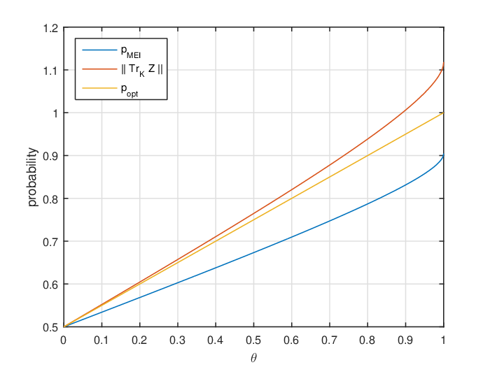
To underline how maximally entangled input states may be used for discrimination of two qubit channels, we will present an example of discrimination of identity channel ϕi​d\phi_{id} and amplitude damping channel ϕA​D\phi_{AD}. The amplitude damping channels are not unital and hence (MEI) is not necessarily satisfied, and we will see that the maximally entangled state is indeed not optimal. The identity channel may be replaced by a unitary channel with some changes to the following calculations. We will set λ=12\lambda=\frac{1}{2}.

Refer to caption
Figure 1. The dependence of success probability with maximally entangled input state pMEIp_{\text{MEI}}, optimal success probability poptp_{\text{opt}} and the upper bound ‖Tr𝒦​Z‖\|\mathrm{Tr}_{\mathcal{K}}Z\| given by Thm. 2 on the parameter θ\theta in discrimination of the amplitude damping channel ϕA​D\phi_{AD} and the identity channel (Example 2).
Example 2.

Let ℋ\mathcal{H} denote complex Hilbert space with dim(ℋ)=2\dim(\mathcal{H})=2 and |0⟩,|1⟩|0\,\rangle,|1\,\rangle will denote some orthonormal basis of ℋ\mathcal{H}. The amplitude damping channel is represented by Kraus operators AθA_{\theta}, BθB_{\theta}, defined as

Aθ\displaystyle A_{\theta} =|0⟩​⟨ 0|+1−θ|1⟩​⟨ 1|,\displaystyle=|0\,\rangle\langle\,0|+\sqrt{1-\theta}|1\,\rangle\langle\,1|,
Bθ\displaystyle B_{\theta} =θ​|0⟩​⟨ 1|,\displaystyle=\sqrt{\theta}|0\,\rangle\langle\,1|,

where θ∈[0,1]\theta\in[0,1] is a parameter. Note that for θ=0\theta=0 the amplitude damping channel becomes the identity. We will proceed as follows: we will find the Choi matrices corresponding to ϕi​d\phi_{id} and ϕA​D\phi_{AD} to obtain pMEIp_{\text{MEI}} and the upper bound on the optimal success probability. Then we will find poptp_{\text{opt}} to compare it with the upper bound.

Let Ci​d=C⁡(ϕi​d)C_{id}=C(\phi_{id}) and CA​D=C⁡(ϕA​D)C_{AD}=C(\phi_{AD}). We will be interested in the matrix Δ12=12​(Ci​d−CA​D)\Delta_{\frac{1}{2}}=\dfrac{1}{2}(C_{id}-C_{AD}) which is of the form

Δ12=12​(0001−1−θ000000−θ01−1−θ00θ).\Delta_{\frac{1}{2}}=\dfrac{1}{2}\begin{pmatrix}0&0&0&1-\sqrt{1-\theta}\\ 0&0&0&0\\ 0&0&-\theta&0\\ 1-\sqrt{1-\theta}&0&0&\theta\end{pmatrix}.

Since pMEI=12​(1+12​Tr​|Δ12|)p_{\text{MEI}}=\frac{1}{2}(1+\frac{1}{2}\mathrm{Tr}\,|\Delta_{\frac{1}{2}}|) we can already find pMEIp_{\text{MEI}} as a function of θ\theta. It is easy to see that 00 and −12​θ-\frac{1}{2}\theta are eigenvalues of Δ12\Delta_{\frac{1}{2}}. Finding the other two eigenvalues is easy since the problem reduces to finding eigenvalues of a 2×22\times 2 matrix, they are 14​(θ+θ2+4​(1−1−θ)2)\frac{1}{4}\big(\theta+\sqrt{\theta^{2}+4(1-\sqrt{1-\theta})^{2}}\,\big) and 14​(θ−θ2+4​(1−1−θ)2)\frac{1}{4}\big(\theta-\sqrt{\theta^{2}+4(1-\sqrt{1-\theta})^{2}}\,\big). Let us denote

λ1=12​(θ+θ2+4​(1−1−θ)2)\displaystyle\lambda_{1}=\frac{1}{2}\big(\theta+\sqrt{\theta^{2}+4(1-\sqrt{1-\theta})^{2}}\,\big)
λ2=12​(θ−θ2+4​(1−1−θ)2)\displaystyle\lambda_{2}=\frac{1}{2}\big(\theta-\sqrt{\theta^{2}+4(1-\sqrt{1-\theta})^{2}}\,\big)

then we have pMEI=12​(1+12​λ1)p_{\text{MEI}}=\frac{1}{2}(1+\frac{1}{2}\lambda_{1}). Moreover after a tedious calculation it can be seen that

Tr1​|Δ12|=\displaystyle\mathrm{Tr}_{1}|\Delta_{\frac{1}{2}}|= λ12​I−λ12+λ1​λ22​(λ1−λ2)​|0⟩​⟨ 0|\displaystyle\dfrac{\lambda_{1}}{2}I-\dfrac{\lambda_{1}^{2}+\lambda_{1}\lambda_{2}}{2(\lambda_{1}-\lambda_{2})}|0\,\rangle\langle\,0|
+λ12+λ1​λ22​(λ1−λ2)​|1⟩​⟨ 1|\displaystyle+\dfrac{\lambda_{1}^{2}+\lambda_{1}\lambda_{2}}{2(\lambda_{1}-\lambda_{2})}|1\,\rangle\langle\,1|

and we have popt≤12​‖I+Tr1​|Δ12|‖p_{\text{opt}}\leq\frac{1}{2}\|I+\mathrm{Tr}_{1}|\Delta_{\frac{1}{2}}|\|. Since λ1≥0\lambda_{1}\geq 0 and λ1±λ2≥0\lambda_{1}\pm\lambda_{2}\geq 0 we have

popt≤12+λ14​(1+θθ2+4​(1−1−θ)2)p_{\text{opt}}\leq\dfrac{1}{2}+\dfrac{\lambda_{1}}{4}\left(1+\dfrac{\theta}{\sqrt{\theta^{2}+4(1-\sqrt{1-\theta})^{2}}}\right)

To verify the upper bound will find poptp_{\text{opt}}, for which we only need to find the value of 12​‖ϕi​d−ϕA​D‖⋄\frac{1}{2}\|\phi_{id}-\phi_{AD}\|_{\diamond}, which we have done by numeric methods. According to [25] the problem of finding a diamond norm can be formulated as following SDP problem:

maxX⁡12​(Tr⁡(Δ12∗​X)+Tr⁡(Δ12​X))\displaystyle\max_{X}\dfrac{1}{2}(\mathrm{Tr}\,(\Delta_{\frac{1}{2}}^{*}X)+\mathrm{Tr}\,(\Delta_{\frac{1}{2}}X))
s.t. ​(I⊗ρ0XX∗I⊗ρ1)\displaystyle\mbox{s.t. }\ \begin{pmatrix}I\otimes\rho_{0}&X\\ X^{*}&I\otimes\rho_{1}\end{pmatrix} ≥0,\displaystyle\geq 0,

where X∈B⁡(ℋ⊗ℋ)X\in B(\mathcal{H}\otimes\mathcal{H}), ρ0,ρ1∈𝔖⁡(ℋ)\rho_{0},\rho_{1}\in\mathfrak{S}(\mathcal{H}). We used MATLAB and the package CVX for solving the convex program, [10, 11]. We have computed the numerical values for 100100 values of the parameter θ\theta, homogeneously distributed on the interval [0,1][0,1]. Between these points straights lines were drawn, hence the figure looks like a continuous line.

The resulting expressions of pMEIp_{\text{MEI}}, ‖Tr𝒦​Z‖\|\mathrm{Tr}_{\mathcal{K}}Z\| and numerical data of poptp_{\text{opt}} as functions of θ\theta are plotted in the Fig. 1. Even though it shows that maximally entangled input state is not optimal, notice that the upper bound is close to po​p​tp_{opt} for small values of the parameter θ\theta.

5.2. Unitary channels

Refer to caption
Figure 2. The dependence of success probability with maximally entangled input state pMEIp_{\text{MEI}}, optimal success probability poptp_{\text{opt}} and the upper bound ‖Tr𝒦​Z‖\|\mathrm{Tr}_{\mathcal{K}}Z\| given by Thm. 2 on the parameter ξ\xi in discrimination of the unitary channel (26) and the identity (Example 3).
Example 3.

Let λ=1/2\lambda=1/2 and dim(ℋ)=3\dim(\mathcal{H})=3. Without loss of generality, we may always assume that we discriminate the identity channel against a unitary A​dWAd_{W}. As our first example, we consider the unitary matrix

(26) W1=(1000i000ei​ξ).W_{1}=\begin{pmatrix}1&0&0\\ 0&i&0\\ 0&0&e^{i\xi}\end{pmatrix}.

At this point, it is easy to compute pMEIp_{\text{MEI}} and ‖Tr𝒦​Z‖\|\mathrm{Tr}_{\mathcal{K}}Z\|, as we can express them as functions of W1W_{1}, which is only dependent on ξ\xi, so the bounds are functions of ξ\xi. Moreover it is possible to compute poptp_{\text{opt}} by numerical methods described in Example 2. The expressions for pMEIp_{\text{MEI}} and ‖Tr𝒦​Z‖\|\mathrm{Tr}_{\mathcal{K}}Z\| are long and messy, they are plotted in the Fig. 2 as well as the computed values of poptp_{\text{opt}}. From the figure it is once again clear that on one hand as pMEIp_{\text{MEI}} rises the the upper bound becomes meaningless, but on the other hand if pMEIp_{\text{MEI}} is small then the upper bound and poptp_{\text{opt}} is small as well.

Another case we consider is matrix of the form

(27) W2=(100012​(1+i)000ei​ξ).W_{2}=\begin{pmatrix}1&0&0\\ 0&\frac{1}{\sqrt{2}}(1+i)&0\\ 0&0&e^{i\xi}\end{pmatrix}.

Again, it is straightforward to obtain pMEIp_{\text{MEI}} and ‖Tr𝒦​Z‖\|\mathrm{Tr}_{\mathcal{K}}Z\| and to compute poptp_{\text{opt}} numerically, the obtained functions are plotted in Fig. 3. Again it can be nicely seen that as pMEIp_{\text{MEI}} rises towards 11 the upper bound becomes meaningless.

Refer to caption
Figure 3. The dependence of success probability with maximally entangled input state pMEIp_{\text{MEI}}, optimal success probability poptp_{\text{opt}} and the upper bound ‖Tr𝒦​Z‖\|\mathrm{Tr}_{\mathcal{K}}Z\| given by Thm. 2 on the parameter ξ\xi in discrimination of the unitary channel (27) and the identity (Example 3).

5.3. Simple projective measurements

Let us demonstrate our results once more, this time for simple projective measurements.

Example 4.

Let λ=12\lambda=\frac{1}{2}, dim(ℋ)≥3\dim(\mathcal{H})\geq 3, |η1⟩=12​(|ξ1⟩+|ξ2⟩)|\eta_{1}\,\rangle=\frac{1}{\sqrt{2}}(|\xi_{1}\,\rangle+|\xi_{2}\,\rangle), |η2⟩=12​(|ξ1⟩−|ξ2⟩)|\eta_{2}\,\rangle=\frac{1}{\sqrt{2}}(|\xi_{1}\,\rangle-|\xi_{2}\,\rangle), |ηj⟩=|ξj⟩|\eta_{j}\,\rangle=|\xi_{j}\,\rangle for j≥3j\geq 3. According to our previous results the maximally entangled input state is not optimal for discriminating these two measurements. As first we need to find Tr𝒦​|Δ12|=12​∑i|Pξi−Pηi|\mathrm{Tr}_{\mathcal{K}}|\Delta_{\frac{1}{2}}|=\frac{1}{2}\sum_{i}|P_{\xi_{i}}-P_{\eta_{i}}|. We get

|Pξ1−Pη1|\displaystyle|P_{\xi_{1}}-P_{\eta_{1}}| =12​|Pξ1−Pξ2−|ξ1⟩​⟨ξ2|−|ξ2⟩​⟨ξ1||,\displaystyle=\dfrac{1}{2}|P_{\xi_{1}}-P_{\xi_{2}}-|\xi_{1}\,\rangle\langle\,\xi_{2}|-|\xi_{2}\,\rangle\langle\,\xi_{1}||,
|Pξ2−Pη2|\displaystyle|P_{\xi_{2}}-P_{\eta_{2}}| =12​|Pξ2−Pξ1+|ξ1⟩​⟨ξ2|+|ξ2⟩​⟨ξ1||,\displaystyle=\dfrac{1}{2}|P_{\xi_{2}}-P_{\xi_{1}}+|\xi_{1}\,\rangle\langle\,\xi_{2}|+|\xi_{2}\,\rangle\langle\,\xi_{1}||,

from which we see, that |Pξ1−Pη1|=|Pξ2−Pη2||P_{\xi_{1}}-P_{\eta_{1}}|=|P_{\xi_{2}}-P_{\eta_{2}}|. The operator Pξ2−Pη2P_{\xi_{2}}-P_{\eta_{2}} is diagonal in the orthonormal basis |φi⟩|\varphi_{i}\,\rangle, i=1,…,dim(ℋ)i=1,\ldots,\dim(\mathcal{H}), where

|φ1⟩\displaystyle|\varphi_{1}\,\rangle =12​2−2​(|ξ1⟩+(1−2)​|ξ2⟩),\displaystyle=\dfrac{1}{\sqrt{2}\sqrt{2-\sqrt{2}}}\left(|\xi_{1}\,\rangle+(1-\sqrt{2})|\xi_{2}\,\rangle\right),
|φ2⟩\displaystyle|\varphi_{2}\,\rangle =12​2+2​(|ξ1⟩+(1+2)​|ξ2⟩),\displaystyle=\dfrac{1}{\sqrt{2}\sqrt{2+\sqrt{2}}}\left(|\xi_{1}\,\rangle+(1+\sqrt{2})|\xi_{2}\,\rangle\right),
|φj⟩\displaystyle|\varphi_{j}\,\rangle =|ξj⟩,\displaystyle=|\xi_{j}\,\rangle,

where j≥3j\geq 3. In this basis it holds that

Pξ1−Pη1=12​Pφ1−12​Pφ2.P_{\xi_{1}}-P_{\eta_{1}}=\dfrac{1}{\sqrt{2}}P_{\varphi_{1}}-\dfrac{1}{\sqrt{2}}P_{\varphi_{2}}.

The following calculation is straightforward. We obtain

Tr𝒦​|Δ12|=12​(Pφ1+Pφ2),\mathrm{Tr}_{\mathcal{K}}|\Delta_{\frac{1}{2}}|=\dfrac{1}{\sqrt{2}}(P_{\varphi_{1}}+P_{\varphi_{2}}),

Now it is easy to see that

pMEI\displaystyle p_{\text{MEI}} =12+12​dim(ℋ),\displaystyle=\dfrac{1}{2}+\dfrac{1}{\sqrt{2}\dim(\mathcal{H})},
‖Tr𝒦​Z‖\displaystyle\|\mathrm{Tr}_{\mathcal{K}}Z\| =2+24≈0.8535​…\displaystyle=\dfrac{2+\sqrt{2}}{4}\approx 0.8535\ldots

i.e. the bound is meaningful and the same for all dim(ℋ)\dim(\mathcal{H}), even though pMEIp_{\text{MEI}} tends to 12\frac{1}{2} from above in the formal limit dim(ℋ)→∞\dim(\mathcal{H})\rightarrow\infty.

To underline the correctness of the upper bound we will find the optimal state for discrimination of the channels. Let us denote Φξ\Phi_{\xi}, Φη\Phi_{\eta} the channel corresponding to simple projective measurement corresponding to the set of projectors {Pξi}\{P_{\xi_{i}}\}, {Pηi}\{P_{\eta_{i}}\} respectively and denote P2=Pξ1+Pξ2P_{2}=P_{\xi_{1}}+P_{\xi_{2}}. Notice that the channels Φξ\Phi_{\xi} and Φη\Phi_{\eta} can be separated as follows

Φξ​(ρ)\displaystyle\Phi_{\xi}(\rho) =∑i=12Tr⁡(Pξi​ρ)​Pξi+∑i=3dim(ℋ)Tr⁡(Pξi​ρ)​Pξi\displaystyle=\sum\limits_{i=1}^{2}\mathrm{Tr}\,(P_{\xi_{i}}\rho)P_{\xi_{i}}+\sum\limits_{i=3}^{\dim(\mathcal{H})}\mathrm{Tr}\,(P_{\xi_{i}}\rho)P_{\xi_{i}}
=ϕξ​(ρ)+χ⁡(ρ),\displaystyle=\phi_{\xi}(\rho)+\chi(\rho),
Φη​(ρ)\displaystyle\Phi_{\eta}(\rho) =∑i=12Tr⁡(Pηi​ρ)​Pξi+∑i=3dim(ℋ)Tr⁡(Pξi​ρ)​Pξi\displaystyle=\sum\limits_{i=1}^{2}\mathrm{Tr}\,(P_{\eta_{i}}\rho)P_{\xi_{i}}+\sum\limits_{i=3}^{\dim(\mathcal{H})}\mathrm{Tr}\,(P_{\xi_{i}}\rho)P_{\xi_{i}}
=ϕη​(ρ)+χ⁡(ρ),\displaystyle=\phi_{\eta}(\rho)+\chi(\rho),

where ρ\rho is a state on ℋ\mathcal{H} and ϕξ=∑i=12Tr⁡(Pξi​ρ)​Pξi\phi_{\xi}=\sum_{i=1}^{2}\mathrm{Tr}\,(P_{\xi_{i}}\rho)P_{\xi_{i}}, ϕη=∑i=12Tr⁡(Pηi​ρ)​Pξi\phi_{\eta}=\sum_{i=1}^{2}\mathrm{Tr}\,(P_{\eta_{i}}\rho)P_{\xi_{i}} and χ=∑i=3dim(ℋ)Tr⁡(Pξi​ρ)​Pξi\chi=\sum_{i=3}^{\dim(\mathcal{H})}\mathrm{Tr}\,(P_{\xi_{i}}\rho)P_{\xi_{i}}. Notice that

ϕξ​(ρ)\displaystyle\phi_{\xi}(\rho) =ϕξ​(P2​ρ​P2),\displaystyle=\phi_{\xi}(P_{2}\rho P_{2}), ϕξ​(P2⟂​ρ​P2⟂)=0,\displaystyle\phi_{\xi}(P_{2}^{\perp}\rho P_{2}^{\perp})=0,
ϕη​(ρ)\displaystyle\phi_{\eta}(\rho) =ϕη​(P2​ρ​P2),\displaystyle=\phi_{\eta}(P_{2}\rho P_{2}), ϕη​(P2⟂​ρ​P2⟂)=0,\displaystyle\phi_{\eta}(P_{2}^{\perp}\rho P_{2}^{\perp})=0,
χ⁡(ρ)\displaystyle\chi(\rho) =χ⁡(P2⟂​ρ​P2⟂),\displaystyle=\chi(P_{2}^{\perp}\rho P_{2}^{\perp}), χ⁡(P2​ρ​P2)=0,\displaystyle\chi(P_{2}\rho P_{2})=0,

where P2⟂=I−P2P_{2}^{\perp}=I-P_{2}. This leads to the following

Φξ​(ρ)=Φξ​(P2​ρ​P2+P2⟂​ρ​P2⟂),\displaystyle\Phi_{\xi}(\rho)=\Phi_{\xi}(P_{2}\rho P_{2}+P_{2}^{\perp}\rho P_{2}^{\perp}),
Φη​(ρ)=Φη​(P2​ρ​P2+P2⟂​ρ​P2⟂).\displaystyle\Phi_{\eta}(\rho)=\Phi_{\eta}(P_{2}\rho P_{2}+P_{2}^{\perp}\rho P_{2}^{\perp}).

In other words, it is sufficient to consider only input states of the form ρ=λ′​ρ2+(1−λ′)​ρ⟂\rho=\lambda^{\prime}\rho_{2}+(1-\lambda^{\prime})\rho_{\perp}, where ρ2\rho_{2} and ρ⟂\rho^{\perp} are states, such that P2​ρ2​P2=ρ2P_{2}\rho_{2}P_{2}=\rho_{2}, P2⟂​ρ⟂​P2⟂=ρ⟂P_{2}^{\perp}\rho_{\perp}P_{2}^{\perp}=\rho_{\perp} and 0≤λ′≤10\leq\lambda^{\prime}\leq 1. Since

popt=\displaystyle p_{\text{opt}}= max⁡(12​Tr​((Φξ⊗i​d)​(ρ)​M)CLOSE\displaystyle\max\left(\dfrac{1}{2}\mathrm{Tr}\,((\Phi_{\xi}\otimes id)(\rho)M)\right.
OPEN+12​Tr​((Φη⊗i​d)​(ρ)​(I−M)))\displaystyle+\left.\dfrac{1}{2}\mathrm{Tr}\,((\Phi_{\eta}\otimes id)(\rho)(I-M))\right)
=\displaystyle= max(λ2(1+Tr(((ϕξ⊗id)(ρ2)\displaystyle\max\left(\dfrac{\lambda}{2}\Big(1+\mathrm{Tr}\,\big(((\phi_{\xi}\otimes id)(\rho_{2})\right.
−(ϕη⊗id)(ρ2))+))+1−λ2),\displaystyle-\left.(\phi_{\eta}\otimes id)(\rho_{2}))_{+}\big)\Big)+\dfrac{1-\lambda}{2}\right),

where MM, I−MI-M is the POVM we use for discrimination of the channels, it is obvious that for poptp_{\text{opt}} to be maximal we also have to set λ=1\lambda=1 and according to corollary 2 the problem reduces to discriminating the channels ϕξ\phi_{\xi} and ϕη\phi_{\eta}. Both ϕξ\phi_{\xi} and ϕη\phi_{\eta} are unital qubit channels and by our previous results the optimal input state ρo​p​t\rho_{opt} is

ρo​p​t=12​∑i,j=12|ξi⟩​⟨ξj|⊗|ξi⟩​⟨ξj|.\rho_{opt}=\dfrac{1}{2}\sum\limits_{i,j=1}^{2}|\xi_{i}\,\rangle\langle\,\xi_{j}|\otimes|\xi_{i}\,\rangle\langle\,\xi_{j}|.

In the product basis given by |ξ1⟩|\xi_{1}\,\rangle, ξ2⟩\xi_{2}\,\rangle, we have

(ϕξ⊗i​d)​(ρo​p​t)−(ϕη⊗i​d)​(ρo​p​t)=\displaystyle(\phi_{\xi}\otimes id)(\rho_{opt})-(\phi_{\eta}\otimes id)(\rho_{opt})=
14​(1−100−1−10000−110011)\displaystyle\dfrac{1}{4}\begin{pmatrix}1&-1&0&0\\ -1&-1&0&0\\ 0&0&-1&1\\ 0&0&1&1\\ \end{pmatrix}

This matrix has two eigenvalues 12​2\frac{1}{2\sqrt{2}} and −12​2-\frac{1}{2\sqrt{2}} each with multiplicity 22. We get Tr⁡(((ϕξ⊗i​d)​(ρ2)−(ϕη⊗i​d)​(ρ2))+)=12\mathrm{Tr}\,\big(((\phi_{\xi}\otimes id)(\rho_{2})-(\phi_{\eta}\otimes id)(\rho_{2}))_{+}\big)=\frac{1}{\sqrt{2}} and

popt=12​(1+12)=2+24p_{\text{opt}}=\dfrac{1}{2}\left(1+\dfrac{1}{\sqrt{2}}\right)=\dfrac{2+\sqrt{2}}{4}

which is exactly the same as our upper bound.

6. Conclusions

We presented necessary and sufficient conditions for optimality of a process POVM in channel discrimination, especially for a process POVM corresponding to a measurement scheme with full Schmidt rank input state. In particular, a necessary and sufficient condition for existence of an optimal measurement scheme with a given full Schmidt rank input state were found. In the case of maximally entangled input states, an upper bound of the optimal success probability was given if the optimality condition is not satisfied. For discrimination of two channels, we obtained a simple condition in terms of the Choi matrices of the channels and a new upper bound on the diamond norm.

The results were applied to discrimination of four types of channels. For covariant channels, known results for the irreducible case were extended to some reducible cases and an upper bound on the optimal success probability was found. For qubit channels, the obtained condition generalizes previously known results to some pairs of non-unital channels. We proved that for discrimination of unitary channels, maximally entangled input states are optimal only in some very special cases. To our best knowledge, the results obtained for unitary channels and simple projective measurements are new.

An interesting open question is whether it is possible to obtain a similar condition for input states with lower Schmidt rank. As it was shown, there are cases when such input states are optimal and there may even be no optimal full rank input states. It is not only of question what the Schmidt rank of the optimal input state may be but also how to select the subspace of the input Hilbert space that will form the support of the partial trace of the input state. Another possible future directions of research is to investigate optimal discrimination of more complex quantum processes.

Acknowledgments

We thank the anonymous referee for the valuable feedback and comments that made this paper more readable and better organized and also for pointing out an easier proof of Prop. 3. This research was supported by grant VEGA 2/0069/16.

References

  • [1] S. M. Barnett and S. Croke, Quantum state discrimination, Adv. Opt. Photonics, vol. 1, no. 2, pp. 238 - 278 (2009)
  • [2] A. O. Barut, R. R\textpolhookaczka, Theory of Group Represetations and Applications, Warszava: PWN - Polish Scientific Publishers, 1980
  • [3] A. Barvinok, A Course in Convexity, AMS, 2002
  • [4] F.G.S.L. Brandao, M. Piani, P. Horodecki, Nature Communications 6, Art. No. 7908 (2015)
  • [5] G. M. D’Ariano, P.LO Presti, M. G. A. Paris, Phys. Rev. Lett. 87, 270404 (2001)
  • [6] G. M. D’Ariano, P.LO Presti, M. G. A. Paris, J. Opt. B 4, 273 (2002)
  • [7] G. Chiribella, Optimal networks for quantum metrology: Semidefinite programs and product rules, New J. Phys., vol. 14, pp. 1-19, (2012)
  • [8] G. Chiribella, G. M. D’Ariano, and P. Perinotti, Phys. Rev. Lett. 101, 180501 (2008)
  • [9] M.D. Choi, Completely positive maps on complex matrices, Lin. Alg. Appl. 10, pp. 285-290 (1975)
  • [10] CVX Research, Inc. CVX: Matlab software for disciplined convex programming, version 2.1. http://cvxr.com/cvx, June 2015.
  • [11] M. Grant, S. Boyd, Graph implementations for nonsmooth convex programs, Recent Advances in Learning and Control (a tribute to M. Vidyasagar), V. Blondel, S. Boyd, and H. Kimura, editors, pp. 95-110, Lecture Notes in Control and Information Sciences, Springer, 2008.
  • [12] Gus Gutoski, J. Math. Phys., vol. 53, no. 3, (2012)
  • [13] Gus Gutoski and John Watrous, Toward a general theory of quantum games. In Proceedings STOC 2007, pp. 565–574
  • [14] C. W. Helstrom, Quantum Detection and Estimation Theory, Academic Press, 1976
  • [15] A. S. Holevo, Journal of Multivariate Analysis 3, pp. 337–394 (1973)
  • [16] A. Jenčová, J Math. Phys. 55, 022201 (2014)
  • [17] A. Kitaev, Quantum computations: algorithms and error correction. Russian Mathematical Surveys, 52, pp. 1191–1249 (1997)
  • [18] K. Matsumoto, arXiv:1209.2392
  • [19] M. Piani and J. Watrous, Phys. Rev. Lett., 102 (25) : 250501, (2009)
  • [20] M. F. Sacchi, Optimal discrimination of quantum operations, Phys. Rev. A 71, 062340 (2005);
  • [21] M. F. Sacchi, Entanglement can enhance the distinguishability of entanglement-breaking channels, Phys. Rev. A - At. Mol. Opt. Phys., vol. 72, no. 1, pp. 1–2 (2005)
  • [22] M. F. Sacchi, Minimum error discrimination of Pauli channels, J. Opt. B-Quantum Semiclassical Opt., vol. 7, no. 10, pp. S333–S336 (2005)
  • [23] M. Sedlák, M. Ziman, Phys. Rev. A 90, 052312 (2014)
  • [24] W. Tadej and K. Zyczkowski, Open Systems and Information Dynamics, vol. 13, pp. 133 - 177 (2006)
  • [25] J. Watrous, Chicago Journal of Theoretical Computer Science, vol. 2013, pp. 1 - 19 (2013)
  • [26] H. Yuen, R. Kennedy and M. Lax, IEEE Transactions on Information Theory, IT-21 (1975)
  • [27] M. Ziman, Phys. Rev. A 77, 062112 (2008)

Appendix: Computation of the absolute value of the difference of positive rank-1 operators

Let |ϕ⟩,|ψ⟩|\phi\,\rangle,|\psi\,\rangle be unit vectors, Pϕ=|ϕ⟩​⟨ϕ|P_{\phi}=|\phi\,\rangle\langle\,\phi|, Pψ=|ψ⟩​⟨ψ|P_{\psi}=|\psi\,\rangle\langle\,\psi|. Let λ∈(0,1)\lambda\in(0,1) and

Dλ:=λ​Pψ−(1−λ)​Pϕ.D_{\lambda}:=\lambda P_{\psi}-(1-\lambda)P_{\phi}.

Then

|Dλ|=|μ1|​Pξ1+|μ2|​Pξ2,|D_{\lambda}|=|\mu_{1}|P_{\xi_{1}}+|\mu_{2}|P_{\xi_{2}},

where μ1,μ2∈ℝ\mu_{1},\mu_{2}\in\mathbb{R} are the eigenvalues and ξ1,ξ2\xi_{1},\xi_{2} the corresponding eigenvectors of DλD_{\lambda}. Moreover, we have

ξi=αiϕ+βiψ,i=1,2\xi_{i}=\alpha_{i}\phi+\beta_{i}\psi,\qquad i=1,2

and since we do not worry about a phase, we may suppose that αi≥0\alpha_{i}\geq 0. From Dλ​|ξi⟩=μi​|ξi⟩D_{\lambda}|\xi_{i}\,\rangle=\mu_{i}|\xi_{i}\,\rangle, we obtain

λ⁡(αi​z¯+βi)​|ψ⟩−(1−λ)​(αi+βi​z)​|ϕ⟩=\displaystyle\lambda(\alpha_{i}\bar{z}+\beta_{i})|\psi\,\rangle-(1-\lambda)(\alpha_{i}+\beta_{i}z)|\phi\,\rangle=
μi​αi​|ϕ⟩+μi​βi​|ψ⟩,\displaystyle\mu_{i}\alpha_{i}|\phi\,\rangle+\mu_{i}\beta_{i}|\psi\,\rangle,

where z=⟨ϕ,ψ⟩z=\langle\,\phi,\psi\,\rangle. It follows that λ⁡(αi​z¯+βi)=μi​βi\lambda(\alpha_{i}\bar{z}+\beta_{i})=\mu_{i}\beta_{i}, so that

βi=kiz¯,i=1,2\beta_{i}=k_{i}\bar{z},\qquad i=1,2

where ki=λμi−λ​αi∈ℝk_{i}=\frac{\lambda}{\mu_{i}-\lambda}\alpha_{i}\in\mathbb{R}. We obtain

|Dλ|=\displaystyle|D_{\lambda}|= ∑i=12|μi|​|αi​ϕ+ki​z¯​ψ⟩​⟨αi​ϕ+ki​z¯​ψ|\displaystyle\sum_{i=1}^{2}|\mu_{i}||\alpha_{i}\phi+k_{i}\bar{z}\psi\,\rangle\langle\,\alpha_{i}\phi+k_{i}\bar{z}\psi|
=\displaystyle= ∑i=12|μi|(αi2​Pϕ+ki2​|z|2​PψCLOSE\displaystyle\sum_{i=1}^{2}|\mu_{i}|(\alpha_{i}^{2}P_{\phi}+k_{i}^{2}|z|^{2}P_{\psi}
OPEN+αi​ki​z​|ϕ⟩​⟨ψ|+αi​ki​z¯|ψ⟩​⟨ϕ|)\displaystyle+\alpha_{i}k_{i}z|\phi\,\rangle\langle\,\psi|+\alpha_{i}k_{i}\bar{z}|\psi\,\rangle\langle\,\phi|)
=\displaystyle= (|μ1|​α12+|μ2|​α22)​Pϕ\displaystyle(|\mu_{1}|\alpha_{1}^{2}+|\mu_{2}|\alpha_{2}^{2})P_{\phi}
+(|μ1|​k12+|μ2|​k22)​|z|2​Pψ+(α1​k1​|μ1|CLOSE\displaystyle+(|\mu_{1}|k_{1}^{2}+|\mu_{2}|k_{2}^{2})|z|^{2}P_{\psi}+(\alpha_{1}k_{1}|\mu_{1}|
OPEN+α2​k2​|μ2|)​(z⁡|ϕ⟩​⟨ψ|+z¯|ψ⟩​⟨ϕ|).\displaystyle+\alpha_{2}k_{2}|\mu_{2}|)(z|\phi\,\rangle\langle\,\psi|+\bar{z}|\psi\,\rangle\langle\,\phi|).