Minimization of Büchi Automata using Fair Simulation

Bachelorthesis

Daniel Tischner

Abstract

We present an algorithm, which reduces the size of Büchi automata using fair simulation. Its time complexity is $\mathcal{O}(|Q|^{4}\cdot|\Delta|^{2})$ , the space complexity is $\mathcal{O}(|Q|\cdot|\Delta|)$ .

Simulation is a common approach for minimizing $\omega$ -automata such as Büchi automata. Direct simulation, delayed simulation and fair simulation are different types of simulation. As we will show, minimization based on direct or delayed simulation is conceptually simple. Whereas the algorithm based on fair simulation is more complex. However, fair simulation allows a stronger minimization of the automaton.

Further, we illustrate the theory behind the algorithm, cover optimizations useful in practice, give experimental results and compare our technique to other minimization strategies.

^†^†publishers: Supervisor: Prof. Dr. Andreas Podelski Advisor: Matthias Heizmann

1 Introduction

Many applications heavily make use of automata, as shown in [7, 10, 15]. Büchi automata, alongside LTL, are commonly used for model checking. Efficiently reducing the size of automata without changing their language greatly improves the capabilities of such applications, since the amount of states and transitions often form a bottleneck.

Refer to caption — Fig. 1: Automaton where there is no mutually delayed simulation but three pairs of states that fairly simulate each other, $\{(q_{ri},q_{li})|i\in\mathbb{N}\}$ . The algorithm presented in this thesis (see Section 4) checks whether merging those states changes the language. Since it does not, the merges are accepted. The state $q_{a}$ gets removed because $cccac^{\omega}$ is no accepting word.

The term minimizing an automaton can be used in different ways. For $\omega$ -automata, finding a language-equivalent automaton with minimal size is NP-hard. This was proven in [13]. Instead, in the context of this thesis, it is defined as the search for any language-equivalent automaton with less states and transitions.

A common approach for minimization consists of finding pairs of states that can be merged without changing the language of the automaton. They are called merge-equivalent. But how can those efficiently be found for $\omega$ -automata such as Büchi automata?

Many existing solutions are based on simulation. Moreover, as seen in [6], they use direct simulation or delayed simulation. Simulation provides pairs of states, they are called simulation-equivalent. For direct and delayed simulation such pairs are always also merge-equivalent, as shown in [6]. Unfortunately, these types of simulation are not always practicable. For delayed simulation, they quickly run out of space for big automata. For direct simulation, they just remove few states.

In this work, we present an algorithm first introduced in [7] which reduces the size of Büchi automata using fair simulation. Its time complexity is $\mathcal{O}(|Q|^{4}\cdot|\Delta|^{2})$ , the space complexity is $\mathcal{O}(|Q|\cdot|\Delta|)$ . The state pairs provided by fair simulation are a superset of the pairs provided by direct or delayed simulation. Therefore, a technique based on fair simulation can remove more states than based direct or delayed simulation (compare to Fig. 1). However, in contrast to the other types, merging two fair-simulation equivalent states is not always possible without changing the language of the automaton (see Fig. 2). We present a method which checks if merging two states changes the language with acceptable overhead.

Moreover, the presented algorithm extends techniques of [6] by also removing some transitions redundant for the language of the automaton, as seen in Fig. 3. This approach effectively eliminates entire parts of an automaton which become unreachable after the edge removal.

Besides presenting the algorithm, another focus of this work is to illustrate the theory behind it and to cover optimizations useful in practice. Further we give experimental results as the algorithm runs in the context of the ULTIMATE Project [11], which is a program analysis framework. Additionally we compare our method to other minimization techniques.

2 Simulation

This section presents different types of simulation based on relations, focusing on fair simulation. It first demonstrates how to obtain simulation relations on Büchi automata in general. As an introduction to the minimization algorithm, parity games and parity game graphs are then explained in more detail.

2.1 Preliminaries

Definition 1.

A Büchi automaton $A$ is a tuple $\langle\Sigma,Q,Q_{0},\Delta,F\rangle$ , where $\Sigma$ is a finite set called the alphabet, $Q$ is a finite set of states, $Q_{0}\subseteq Q$ is the set of initial states, $\Delta\subseteq Q\times\Sigma\times Q$ is the transition relation and $F\subseteq Q$ is the set of final states.

We define $succ(v)$ for the set of successors $\{v^{\prime}\in V|\exists a\in\Sigma\,\exists(v,a,v^{\prime})\in\Delta\}$ and $pred(v)$ analogue for the set of predecessors of a given state $v$ .

Given a Büchi automaton $A$ , $A^{q}$ refers to the Büchi automaton
$\langle\Sigma,Q,\{q\},\Delta,F\rangle$ which is the automaton $A$ with only $q$ as initial state.

Definition 2.

A run of a Büchi automaton $A$ is a sequence
$\pi=q_{0}a_{1}q_{1}a_{2}q_{2}a_{3}q_{3}\ldots$ of arbitrary states alternating with arbitrary letters such that $\forall i:(q_{i},a_{i+1},q_{i+1})\in\Delta$ . The run forms the path $q_{0}\overset{a_{1}}{\rightarrow}q_{1}\overset{a_{2}}{\rightarrow}q_{2}\overset{a_{3}}{\rightarrow}q_{3}\ldots$ in $A$ and the corresponding $\omega$ -word is $w=a_{1}a_{2}a_{3}\ldots$ .

We write $q\in\pi$ or $a\in\pi$ if the state or letter occurs at least once in the sequence $\pi$ .

The automaton $A$ accepts an $\omega$ -word $w=a_{1}a_{2}a_{3}\ldots$ iff for at least one corresponding run $\pi$ the following holds:

\displaystyle q_{0}\in Q_{0},\forall i:(q_{i},a_{i+1},q_{i+1})\in\Delta\text{ and }|\{i:q_{i}\in F\}|=\infty,

i.e. $\pi$ starts at an initial state and visits finite states infinitely often.

Definition 3.

The accepted $\omega$ -language of a Büchi automaton $A$ is
$\mathcal{L}(A)=\{w\in\Sigma^{\omega}|A\text{ accepts }w\}$ .

For the sake of simplicity, the presented algorithm requires $A$ to have no dead ends.

Definition 4.

A dead end is a state of an automaton $A$ that has no outgoing transitions, i.e. $v$ dead end $\Leftrightarrow v\in Q\land succ(v)=\emptyset$ .

However, Section 5 shows how automata with dead ends are handled. Fig. 4 shows an automaton and its language, and illustrates several runs with their corresponding words and a dead state.

2.2 Types of simulation

Definition 5.

Given a Büchi automaton $A$ , fair simulation is defined as a relation $\preceq_{f}\,\subseteq Q\times Q$ where

	$\displaystyle q\preceq_{f}q^{\prime}\text{ iff }$	$\displaystyle\left(\forall w=a_{1}a_{2}\ldots\exists\pi=qa_{1}q_{1}a_{2}\ldots\Rightarrow\exists\pi^{\prime}=q^{\prime}a_{1}q^{\prime}_{1}a_{2}\ldots\right)$
		$\displaystyle\land\left(\forall w=a_{1}a_{2}\ldots\in\mathcal{L}(A^{q})\Rightarrow w\in\mathcal{L}(A^{q^{\prime}})\right).$

I.e. for all words that have a corresponding run starting at $q$ , there must also be a corresponding run to the same word starting at $q^{\prime}$ . And, for all accepting words whose runs start at $q$ , there must also exist an accepting run starting at $q^{\prime}$ that corresponds to the same word.

Let $\pi=q_{0}a_{1}q_{1}a_{2}q_{2}a_{3}q_{3}\ldots$ and $\pi^{\prime}=q^{\prime}_{0}a_{1}q^{\prime}_{1}a_{2}q^{\prime}_{2}a_{3}q^{\prime}_{3}\ldots$ be corresponding runs to $w$ starting at $q=q_{0}$ and $q^{\prime}=q^{\prime}_{0}$ . Then delayed simulation is a relation $\preceq_{de}\,\subseteq Q\times Q$ where

\displaystyle q\preceq_{de}q^{\prime}\text{ iff }q\preceq_{f}q^{\prime}\land\forall i:q_{i}\in F\Rightarrow\exists j\geq i:q^{\prime}_{j}\in F.

Every time $\pi$ visits an accepting state $q_{i}$ , $\pi^{\prime}$ must also visit at least one accepting state $q^{\prime}_{j}$ at some point after to cover that event.

3.

Direct simulation is defined analogously,

$\displaystyle q\preceq_{di}q^{\prime}\text{ iff }q\preceq_{f}q^{\prime}\land\forall i:q_{i}\in F\Rightarrow q^{\prime}_{i}\in F.$

That is, every time $\pi$ visits an accepting state $q_{i}$ , $\pi^{\prime}$ must also visit an accepting state $q^{\prime}_{i}$ at the same time.

We say $q^{\prime}$ $\star$ -simulates $q$ if the relation $q\preceq_{\star}q^{\prime}$ , where $\star\in\{f,de,di\}$ , holds. Note that $q\preceq_{di}q^{\prime}\Rightarrow q\preceq_{de}q^{\prime}\Rightarrow q\preceq_{f}q^{\prime}$ , but not vice versa which follows directly from the definition.

Again taking a look at Fig. 1 reveals that $q_{l1}$ fairly simulates $q_{r1}$ ( $q_{r1}\preceq_{f}q_{l1}$ ) and vice versa. The run starting at the state $q_{r1}$ is $\pi_{r1}=q_{r1}cq_{r2}cq_{r3}bq_{b}c\ldots$ , which corresponds to the word $w=ccbc\ldots$ . The run $\pi_{r1}$ is accepting, but there is also an accepting run starting at $q_{l1}$ corresponding to the same word, namely $\pi_{l1}=q_{l1}cq_{l2}cq_{l3}bq_{b}c\ldots$ . Since there are no other accepting runs starting at $q_{r1}$ it follows that $q_{r1}\preceq_{f}q_{l1}$ .

It holds that $q_{r1}$ delayedly and directly simulates $q_{l1}$ . Regardless of whether $\pi_{l1}$ visits $q_{a}$ or $q_{b}$ , everytime it visits an accepting state $\pi_{r1}$ does also. This is because $q_{b}$ is the only accepting state on run $\pi_{l1}$ .

But $q_{l1}$ does not directly simulate $q_{r1}$ . Since $q_{l1},q_{l2},q_{l3}$ are not accepting states, $\pi_{l1}$ cannot visit accepting states the same time $\pi_{r1}$ does.

$q_{l1}$ also not delayedly simulates $q_{r1}$ because the corresponding word $w=ccac\ldots$ of the run $\pi_{r1}=q_{r1}cq_{r2}cq_{r3}aq_{a}c\ldots$ can only be matched by the run $\pi_{l1}=q_{l1}cq_{l2}cq_{l3}aq_{a}c\ldots$ . Further, $\pi_{r1}$ visits three accepting states before entering the loop whereas $\pi_{l1}$ not visits an accepting state for coverage.

Last we point out why $q_{r1}$ does not fairly simulate $q_{r2}$ . The run $\pi_{r2}=q_{r2}cq_{r3}bq_{b}c\ldots$ corresponds to the word $w=cbc\ldots$ , but no run $\pi_{r1}$ corresponding to the same word starting from $q_{r1}$ exists.

For minimizing automata pairs of states that simulate each other, i.e. $q$ and $q^{\prime}$ if $q\preceq_{\star}q^{\prime}\land q^{\prime}\preceq_{\star}q$ are of interest. As seen later, for $\star\in\{di,de\}$ it is always possible to merge such a pair without changing the language of the automaton. For fair simulation this is not always be the case. As the algorithm in question aims to reduce as many states as safely possible, the correctness of any such potential merge must be verified before it is applied.

A naive implementation, for determining whether a pair of states $q$ and $q^{\prime}$ simulates each other, consists of iterating over all possible words starting at $q$ and $q^{\prime}$ . Then creating all corresponding runs for such words and compute wether Definition 5 holds.

We present a more efficient implementation, Algorithm 1. The concept of this algorithm is based on parity games.

2.3 Parity game

A parity game $G_{A}(q,q^{\prime})$ , where $q$ and $q^{\prime}$ are arbitrary states of the Büchi automaton $A$ , is played by two players, Spoiler (or Antagonist) and Duplicator (or Protagonist). Each player has one token, initially placed at states $q$ and $q^{\prime}$ , for Spoiler and Duplicator respectively. The players move their token alongside the automaton $A$ using transitions. Both tokens can be moved to the same state without interfering each other.

The game is played in rounds, assuming that at the beginning of round $i$ Spoiler’s token is at state $q_{i}$ and Duplicator’s at $q^{\prime}_{i}$ , a round is played as follows:

1.

Spoiler chooses a transition $(q_{i},a,q_{i+1})\in\Delta$ and moves his token to $q_{i+1}$ .
2.

Duplicator must now respond to Spoiler’s choice, choose an a-transition $(q^{\prime}_{i},a,q^{\prime}_{i+1})\in\Delta$ and move his token to $q^{\prime}_{i+1}$ .

If $q^{\prime}_{i}$ does not have such an outgoing a-transition, Duplicator can not respond. The game halts and Spoiler wins the game. Note that Spoiler can always choose an outgoing transition, as we assume $A$ having no dead ends (compare to Definition 4).

If Duplicator can always respond to Spoilers choices, the game produces two infinite runs $\pi=qa_{1}q_{1}a_{2}q_{2}a_{3}q_{3}\ldots$ and $\pi^{\prime}=q^{\prime}a_{1}q^{\prime}_{1}a_{2}q^{\prime}_{2}a_{3}q^{\prime}_{3}\ldots$ . The game history is defined as the tuple $(\pi,\pi^{\prime})$ .

We connsider three types of parity games. All of them differ in the winning conditions for Duplicator.

Definition 6.

1.

In the direct simulation game $G^{di}_{A}(q,q^{\prime})$ the game history $(\pi,\pi^{\prime})$ is winning for Duplicator iff $\forall i:q_{i}\in F\Rightarrow q^{\prime}_{i}\in F$ .
2.

In the delayed simulation game $G^{de}_{A}(q,q^{\prime})$ the game history $(\pi,\pi^{\prime})$ is winning for Duplicator iff $\forall i:q_{i}\in F\Rightarrow\exists j>i:q^{\prime}_{j}\in F$ .
3.

In the fair simulation game $G^{f}_{A}(q,q^{\prime})$ the game history $(\pi,\pi^{\prime})$ is winning for Duplicator iff $|\{j|q^{\prime}_{j}\in F\}|=\infty\Rightarrow|\{i|q_{i}\in F\}|<\infty$ .

Note that there are similarities between this definition and the definition of simulation (Definition 5).

Fig. 5 shows two copies of the same automata. They represent a parity game with the token of Spoiler initially standing on $q_{3}$ and the token of Duplicator on $q_{1}$ . Spoiler has two possibilites in the first round, he can choose the $b$ -transition $(q_{3},b,q_{4})$ or the $a$ -transition $(q_{3},a,q_{5})$ . A wise decision would be to choose the $a$ -transition, we assume he decides for this way. The token of Spoiler now is placed at $q_{5}$ and Duplicator must also choose an $a$ -transition or he looses. Duplicator decides for $(q_{1},a,q_{2})$ and moves his token to $q_{2}$ . The second round starts and Spoiler has again the option to choose any transition he likes. However, there is only one transition and he chooses $(q_{5},a,q_{5})$ . Duplicator must react and also choose an $a$ -transition but $q_{2}$ has no outgoing transitions. The game holds and Spoiler wins since Duplicator can not match his transition.

Now assuming Spoiler takes the $b$ -transition in the first round and moves to $q_{4}$ instead of $q_{5}$ . If Duplicator takes the transition $(q_{1},b,q_{2})$ he would lose again in the next round so he chooses $(q_{1},b,q_{3})$ . The only possibility for Spoiler is to take $(q_{4},b,q_{4})$ and Duplicator also moves to $q_{4}$ . Both players now repeatedly take the transition $(q_{4},b,q_{4})$ and the game creates the game history $(\pi,\pi^{\prime})$ where $\pi=q_{3}bq_{4}b\ldots$ and $\pi^{\prime}=q_{1}bq_{3}bq_{4}b\ldots$ . The game history determines the winner, for fair and delayed simulation the game history is winning for Duplicator, for direct simulation Spoiler wins since he visits an accepting state in the first round while Duplicator visits $q_{3}$ in this round.

Observe that as soon as, in the beginning of the same round, Duplicator’s token is placed at the same state Spoiler’s token is at, he can directly copy every move of Spoiler by simply following him. If that is the case Spoiler cannot win the game anymore.

While assuming both players give their best Spoiler would not choose the transition $(q_{3},b,q_{4})$ and Duplicator would not choose $(q_{1},b,q_{2})$ .

2.3.1 Strategy

Informally a stategy for Duplicator determines at each round of the game which transition Duplicator should choose based on the history of previous rounds. Such a strategy is called a winning strategy if, no matter how Spoiler plays, Duplicator always wins. While assuming that Duplicator always gives his best to win this corresponds to using the best strategy. Formally strategy and winning strategy are defined the way as seen in [6].

Definition 7.

Let $s_{i}=q_{0}q^{\prime}_{0}a_{1}q_{1}q^{\prime}_{1}a_{2}\ldots a_{i-1}q_{i-1}q^{\prime}_{i-1}a_{i}q_{i}$ be an interleaving sequence such that $\pi^{\prime}=q_{0}a_{1}q_{1}a_{2}\ldots a_{i-1}q_{i-1}a_{i}q_{i}$ is a run for Spoiler and $\pi=q^{\prime}_{0}a_{1}q^{\prime}_{1}a_{2}\ldots a_{i-1}q^{\prime}_{i-1}$ is a run for Duplicator.

A strategy for Duplicator in $G^{\star}_{A}(q,q^{\prime})$ is a partial function $f:Q\times(Q\times\Sigma\times Q)^{*}\mathrel{\vtop{\halign{#\cr\hfil$\mapstochar$\hfil\cr$\to$\cr}}}Q$ where

\displaystyle f(q)=q^{\prime}\land(\forall s_{i}:i>0\Rightarrow(q^{\prime}_{i-1},a_{i},f(s_{i}))\in\Delta).

Observe that the existance of a strategy implies that it is possible for Duplicator to play the game in such way that it does not halt. It also means that if there does not exist a strategy for Duplicator then Spoiler always wins the game since he can make moves Duplicator cannot respond to.

In the example of Fig. 5 there does not exist a strategy for Duplicator. Since if Spoiler chooses the $a$ -transition $(q_{3},a,q_{5})$ and then $(q_{5},a,q_{5})$ Duplicator, meanwhile at $q_{2}$ , has no possibility to find an outgoing $a$ -transition. The corresponding sequence up to this point is $s_{2}=q_{3}q_{1}aq_{5}q_{2}aq_{5}$ .

Assuming the transition $(q_{3},a,q_{5})$ does not exist, Spoiler must choose the $b$ -transition $(q_{3},b,q_{4})$ , then there exist two different strategies. The first strategy $f_{1}$ chooses $(q_{1},b,q_{2})$ for Duplicator, $f_{1}(q_{3}q_{1}bq_{4})=q_{2}$ and the second strategy $f_{2}$ chooses $(q_{1},b,q_{3})$ , $f_{2}(q_{3}q_{1}bq_{4})=q_{3}$ .

Definition 8.

A strategy $f$ for Duplicator in $G^{\star}_{A}(q,q^{\prime})$ is a winning strategy iff for all runs of Spoiler $\pi$ there exists a run of Duplicator $\pi^{\prime}$ , received by using the strategy for each move, such that the game history $(\pi,\pi^{\prime})$ is winning for Duplicator (Definition 6).

$\forall\pi=q_{0}a_{1}q_{1}a_{2}\ldots\exists\pi^{\prime}:(\pi,\pi^{\prime})$ winning for Duplicator, where run $\pi^{\prime}=q_{0}^{\prime}a_{1}q_{1}^{\prime}a_{2}\ldots$ is the run received by $q^{\prime}_{i+1}=f(q_{0}q^{\prime}_{0}a_{1}q_{1}q^{\prime}_{1}a_{2}\ldots q_{i+1})$ .

Having a winning strategy means that, for fixed starting positions, no matter how Spoiler plays the strategy will always create a winning game history for Duplicator. When using such a strategy for given starting positions it is not possible for Spoiler to win the game.

In Fig. 5, when again assuming $(q_{3},a,q_{5})$ does not exist, there is a winning strategy for fair and delayed simulation games. Strategy $f_{2}$ , which chooses $(q_{1},b,q_{3})$ instead of $(q_{1},b,q_{2})$ is a winning strategy. In complete $f_{2}$ is defined as follows:

$\displaystyle f_{2}$	$\displaystyle(q_{3})$	$\displaystyle=q_{1}$
$\displaystyle f_{2}$	$\displaystyle(q_{3}q_{1}bq_{4})$	$\displaystyle=q_{3}$
$\displaystyle f_{2}$	$\displaystyle(q_{3}q_{1}bq_{4}q_{3}bq_{4})$	$\displaystyle=q_{4}$
$\displaystyle f_{2}$	$\displaystyle(q_{3}q_{1}bq_{4}q_{3}bq_{4}q_{4}bq_{4})$	$\displaystyle=q_{4}$

The following lemma shows the connection between parity games and simulation relations.

Lemma 1.

Given a Büchi automaton $A$ where $q$ and $q^{\prime}$ are states of $A$ ,
$q\preceq_{\star}q^{\prime}$ iff there exists a winning strategy for Duplicator in $G^{\star}_{A}(q,q^{\prime})$ where $\star\in\{di,de,f\}$ .

Proof.

The winning strategy creates game histories $(\pi,\pi^{\prime})$ for every run $\pi$ Spoiler can build. Since the strategy is a winning strategy every run $\pi^{\prime}$ that follows the strategy creates a game history that is winning for Duplicator. Given the definition of such a game history (Definition 6) it follows directly that $q\preceq_{\star}q^{\prime}$ .

Assuming $q\preceq_{\star}q^{\prime}$ there must exist a game history $(\pi,\pi^{\prime})$ that is winning for Duplicator for every possible run $\pi$ Spoiler can create. All possible runs $\pi$ of Spoiler together with the corresponding runs $\pi^{\prime}$ of Duplicator define a winning strategy and the proof is complete.
∎

Given two states $q$ and $q^{\prime}$ , finding out if $q\preceq_{\star}q^{\prime}$ is equivalent to finding a winning strategy for Duplicator in the game $G^{\star}_{A}(q,q^{\prime})$ .

2.4 Parity game graph

Obviously the difficulty is to find a winning strategy or to proof that there does not exist one. By using parity game graphs the problem can be solved algorithmic.

Definition 9.

Let $A=\langle\Sigma,Q,Q_{0},\Delta,F\rangle$ be a Büchi automaton to which we refer as Spoiler’s automaton and $A^{\prime}=\langle\Sigma,Q^{\prime},Q^{\prime}_{0},\Delta^{\prime},F^{\prime}\rangle$ is a Büchi automaton to which we refer as Duplicator’s automaton. A parity game graph on two Büchi automata is a tuple $G^{\star}_{A,A^{\prime}}=\langle V_{0}^{\star},V_{1}^{\star},E^{\star},p^{\star}\rangle$ where $\star\in\{di,de,f\}$ .

$V^{\star}$ is the set of vertices and $V^{\star}=V_{0}^{\star}\cup V_{1}^{\star}$ , $E^{\star}\subseteq V^{\star}\times V^{\star}$ is the set of edges (note that labels for the edges are not needed) and $p^{\star}:V^{\star}\to\mathbb{N}$ is a function that maps a priority to each vertex.

The elements are defined as follows:

1.

For fair simulation ( $\star=f$ ):

$V_{1}^{f}=\{v_{(q,q^{\prime})}|q\in Q\land q^{\prime}\in Q^{\prime}\}$

$V_{0}^{f}=\{v_{(q,q^{\prime},a)}|q\in Q\land q^{\prime}\in Q^{\prime}\land\exists\tilde{q}\in pred(q):(\tilde{q},a,q)\in\Delta\}$

$E^{f}=\underbrace{\{(v_{(q,q^{\prime})},v_{(\tilde{q},q^{\prime},a)})|\exists(q,a,\tilde{q})\in\Delta\}}_{\text{move from Spoiler}}$

$\cup\underbrace{\{(v_{(q,q^{\prime},a)},v_{(q,\tilde{q})})|\exists(q^{\prime},a,\tilde{q})\in\Delta^{\prime}\}}_{\text{move from Duplicator}}$

$p^{f}:V^{f}\to\{0,1,2\},p^{f}(v)=\begin{cases}0&\textnormal{if }v=v_{(q,q^{\prime})}\land q^{\prime}\in F^{\prime}\\ 1&\textnormal{if }v=v_{(q,q^{\prime})}\land q\in F\land q^{\prime}\notin F^{\prime}\\ 2&\textnormal{otherwise}\end{cases}$
2.

For direct simulation ( $\star=di$ ):

$V_{1}^{di}=V_{1}^{f}$

$V_{0}^{di}=V_{0}^{f}$

$E^{di}=E^{f}\setminus(\{(v_{(q,q^{\prime})},v_{(\tilde{q},q^{\prime},a)})|q\in F\land q^{\prime}\notin F^{\prime}\}$

$\cup\{(v_{(q,q^{\prime},a)},v_{(q,\tilde{q})})|q\in F\land\tilde{q}\notin F^{\prime}\})$

$p^{di}:V^{di}\to\{0\},p^{di}(v)=0$
3.

For delayed simulation ( $\star=de$ ):

$V_{1}^{de}=\{v_{(b,q,q^{\prime})}|q\in Q\land q^{\prime}\in Q^{\prime}\land b\in\{0,1\}\land(q^{\prime}\in F^{\prime}\rightarrow b=0)\}$

$V_{0}^{de}=\{v_{(b,q,q^{\prime},a)}|q\in Q\land q^{\prime}\in Q^{\prime}\land b\in\{0,1\}\land\exists\tilde{q}\in pred(q):(\tilde{q},a,q)\in\Delta\}$

$E^{de}=\{v_{(b,q,q^{\prime}),v_{(b,\tilde{q},q^{\prime},a)}}|(q,a,\tilde{q})\in\Delta\land\tilde{q}\notin F\}$

$\cup\{v_{(b,q,q^{\prime}),v_{(1,\tilde{q},q^{\prime},a)}}|(q,a,\tilde{q})\in\Delta\land\tilde{q}\in F\}$

$\cup\{v_{(b,q,q^{\prime},a)},v_{(b,q,\tilde{q})}|(q^{\prime},a,\tilde{q}\in\Delta^{\prime}\land\tilde{q}\notin F^{\prime})\}$

$\cup\{v_{(b,q,q^{\prime},a)},v_{(0,q,\tilde{q})}|(q^{\prime},a,\tilde{q}\in\Delta^{\prime}\land\tilde{q}\in F^{\prime})\}$

$p^{de}:V^{de}\to\{0,1,2\},p^{de}(v)=\begin{cases}b&\textnormal{if }v=v_{(b,q,q^{\prime})}\in V^{de}_{1}\\ 2&\textnormal{if }v\in V^{de}_{0}\end{cases}$
The bit b encodes whether Spoiler has visited a final state without Duplicator visiting one since then, 1 indicates this and 0 the opposite case.

For the remainder of this thesis $(q,q^{\prime})$ abbreviates the vertex $v_{(q,q^{\prime})}$ and $(q,q^{\prime},a)$ the vertex $v_{(q,q^{\prime},a)}$ .

From now the focus is on fair simulation parity game graphs but the same can be applied similiar to other simulations.

First note that a parity game graph is build using two automata $A$ and $A^{\prime}$ . In order to compute simulation relations it is enough to use $A=A^{\prime}$ and simply write $G^{f}_{A}$ instead of $G^{f}_{A,A}$ . But Section 4 needs the possibility to build a game graph on two different automata. This allows letting Spoiler play on a different automaton than Duplicator which makes computing simulation relations between two different automaton possible.

A parity game graph represents all possible positions and moves of a parity game in one graph. For each position of the parity game, the states Spoiler and Duplicator stand on, there is a vertex in the graph. Possible moves of the players are represented by edges between the vertices.

More precisely a vertex $v_{1}=(q,q^{\prime})\in V^{f}_{1}$ or $v_{0}=(q,q^{\prime},a)\in V^{f}_{0}$ encodes the position where Spoiler’s token is placed at $q$ and Duplicator’s at $q^{\prime}$ . For such a vertex $v_{1}$ it is now Spoiler’s time to make a move and choose a transition, he may choose an a-transition $(q,a,\tilde{q})\in\Delta$ which is encoded by the vertex $v_{0}=(\tilde{q},q^{\prime},a)\in V^{f}_{0}$ that stands for the position where Duplicator also needs to choose an a-transition. Let that transition be $(q^{\prime},a,\bar{q})\in\Delta^{\prime}$ which then leads to the vertex $(\tilde{q},\bar{q})\in V^{f}_{1}$ in the game graph. The game graph has edges between vertices for every possible move. For example the edge $(v_{(q,q^{\prime})},v_{(\tilde{q},q^{\prime},a)})$ does exist if it is possible for Spoiler to move from the state $q$ to $\tilde{q}$ by using the letter $a$ , i.e. $(q,a,\tilde{q})\in\Delta$ . And $(v_{(q,q^{\prime},a)},v_{(q,\tilde{q})})$ exists if Duplicator can move from $q^{\prime}$ to $\tilde{q}$ by using $a$ , i.e. $(q^{\prime},a,\tilde{q})\in\Delta^{\prime}$ .

Fig. 6 illustrates the fair simulation game graph $G^{f}_{A,A}$ obtained by using the automaton $A$ (from Fig. 2) for Spoiler and also for Duplicator. When creating a game graph, the transition $(q_{0},a,q_{0})$ from $A$ produces the edges $(v_{(q_{0},q_{0})},v_{(q_{0},q_{0},a)})$ , $(v_{(q_{0},q_{1})},v_{(q_{0},q_{1},a)})$ and $(v_{(q_{0},q_{0},a)},v_{(q_{0},q_{0})})$ in $G^{f}_{A,A}$ . The vertex $v_{(q_{1},q_{0},a)}$ does not exist since it would require $q_{1}$ to have an incoming transition labeled with $a$ .

2.4.1 Correlation to parity games

A parity game $G^{f}_{A}(q,q^{\prime})$ can be played on the corresponding parity game graph by starting at the vertex $(q,q^{\prime})\in V_{1}$ . The two players, with Spoiler starting, now alternately move the same token over the game graph representing the original game.

The priorities encode the simulation conditions. Priority $0$ , for fair simulation, represents the situation where Duplicator visits a final state. Analogously, priority $1$ stands for the position where Spoiler visits a final state and Duplicator does not. Priority $2$ is a neutral situation in which both players do not visit a final state.

Fig. 6 demonstrates the definition of priority for fair simulation. The vertex $v_{(q_{1},q_{1})}$ has a priority of $2$ since $q_{1}$ is no final state, all vertices in $V_{0}$ also have priority $2$ . However, the vertex $v_{(q_{0},q_{1})}$ has priority $1$ because Spoiler’s state $q_{0}$ is final while Duplicator’s state $q_{1}$ is not.

Definition 6 describes that Duplicator wins a parity game if he does not allow Spoiler to visit final states infinitely often, while not doing the same. When Duplicator lost, then he visited vertices with priority $1$ infinitely often by not also visiting priority $0$ that many. So in general Duplicator prefers to visit vertices with priority $0$ and Spoiler prefers priority $1$ since those priorities bring the players closer to their victory. Although this sounds like a good strategy for Duplicator, if he dully moves to a vertex $v$ with priority $0$ , this could lead him into a trap. For example a loop of vertices with priority $1$ behind $v$ or similar.

The following two definitions clarify the connection between parity games and game graphs by introducing an isomorphism $\sigma$ .

Definition 10.

Given the Büchi automata $A,A^{\prime}$ and the game graph $G^{f}_{A,A^{\prime}}$ , let $P$ be the set of all paths in $G^{f}_{A,A^{\prime}}$ , $R$ the set of all runs in $A$ and $R^{\prime}$ of all runs in $A^{\prime}$ .

Then we define the path-transformation $\sigma:P\xrightarrow{\,\smash{\raisebox{-1.35623pt}{$\scriptstyle\sim$}}\,}(R\times R^{\prime})$ . Which is, for a path $\varrho=v_{(q_{0},q^{\prime}_{0})}\rightarrow v_{(q_{1},q^{\prime}_{0},a_{1})}\rightarrow v_{(q_{1},q^{\prime}_{1})}\rightarrow\ldots$ , given by $\sigma(\varrho)=(\pi,\pi^{\prime})$ . Where $\pi=q_{0}a_{1}q_{1}\ldots$ and $\pi^{\prime}=q^{\prime}_{0}a_{1}q^{\prime}_{1}\ldots$ .

Lemma 2.

The path-transformation $\sigma$ is an isomorphism between paths in game graphs and game histories in parity games.

Proof.

$\sigma$ is a morphism by definition. We define $\sigma^{-1}:(R\times R^{\prime})\xrightarrow{\,\smash{\raisebox{-1.35623pt}{$\scriptstyle\sim$}}\,}P$ given by $\sigma^{-1}((\pi,\pi^{\prime}))=\varrho$ where $\pi,\pi^{\prime}$ and $\varrho$ are defined the same as in Definition 10. It follows that $\sigma\circ\sigma^{-1}=\operatorname{id}_{R\times R}$ and $\sigma^{-1}\circ\sigma=\operatorname{id}_{P}$ . Thus $\sigma$ is bijective, an ismorphism and $\sigma^{-1}$ is the inverse of $\sigma$ .
∎

Given the isomorphism $\sigma$ , we define when a path is winning for Duplicator.

Definition 11.

A path $\varrho$ in a game graph $G^{f}_{A,A^{\prime}}$ is winning for Duplicator iff the game history $\sigma(\varrho)$ is winning for Duplicator.

For simplicity $v\in\varrho$ means the path visits a vertex $v$ . With the aid of vertex priorities, the following lemma enhances Definition 11.

Lemma 3.

The path $\varrho$ is winning for Spoiler iff $min\{n:|\{v|v\in\varrho\land p^{f}(v)=n\}|=\infty\}$ is odd, i.e. the smallest priority that occurs infinite times in the path.

Proof.

Spoiler only wins if he visits final states infinitely times while Duplicator does not. This case is reflected by a path that visits vertices with priority $1$ infinitely times while not visiting priority $0$ infinitely often. In all other cases Duplicator wins the game. Since $1$ is the only odd priority, the lemma holds.
∎

Using the path-transformation $\sigma$ and Lemma 3, a winning strategy can be obtained on a parity game graph $G^{f}_{A,A^{\prime}}$ only.

Let us deepen that by again taking a look on Fig. 6. When playing a parity game on the game graph $G^{f}_{A}$ , starting at $(q_{1},q_{1})$ , Spoiler may move to $(q_{1},q_{1},b)$ or $(q_{0},q_{1},a)$ . Assuming he decided for $(q_{1},q_{1},b)$ , Duplicator can only choose $(q_{1},q_{1})$ and it is Spoiler’s turn, again on the same spot. He may choose this edge everytime which produces the path $\varrho=v_{(q_{1},q_{1})}\rightarrow v_{(q_{1},q_{1},b)}\rightarrow v_{(q_{1},q_{1})}\rightarrow\ldots$ . The smallest priority that occurs infinite times on $\varrho$ is $2$ , even both vertices have that priority, which is not odd. Because of that $\varrho$ is winning for Duplicator but Spoiler may choose the transition to $(q_{0},q_{1},a)$ and so on.

In this example, it is not possible for Spoiler to win the play since there is no possibility to visit priority $1$ infinite times no matter where the starting position is or how Duplicator plays. For this reason every strategy for Duplicator is a winning strategy in this game.

The correlation between game graphs and parity games leads to the next observation. With Lemma 1, $\sigma$ and Lemma 3, a simulation relation can be computed on a parity game graph $G^{f}_{A,A^{\prime}}$ only.

Referring to the example of Fig. 6, where every strategy defines a winning strategy, the fair simulation relation is obtained. The relation consists of $q_{0}\preceq_{f}q_{1}$ and $q_{1}\preceq_{f}q_{0}$ . As seen before such a pair that fairly simulates each other is a candidate for merging. However, as seen later, merging $q_{0}$ and $q_{1}$ will change the language of the automaton from $\{w\in\Sigma^{\omega}|w=(b^{*}a)^{\omega}\}$ to $\{w\in\Sigma^{\omega}|w=(ab)^{\omega}\}$ so the merge attempt gets rejected.

3 Computing a simulation relation

In the section before we have seen that $q\preceq_{f}q^{\prime}$ if there exists a winning strategy for Duplicator in the parity game $G^{f}_{A}(q,q^{\prime})$ (see Lemma 1). This section shows how to compute if there exists a winning strategy for a pair of states $q$ and $q^{\prime}$ . A winning strategy is computed on the game graph only by using the isomorphism $\sigma$ (Definition 10) and Lemma 3.

With the use of Jurdzińskis algorithm, originally from [9], the simulation relation is computed for every pair of starting states at the same time. This is done by building paths on the game graph that reflect the optimal solution for the players and extending them in every round if possible. The paths are computed by introducing a progress measure for each vertex.

Given a parity game graph $G^{f}_{A,A^{\prime}}=\langle V_{0},V_{1},E,p\rangle$ on two Büchi automata $A$ and $A^{\prime}$ , in order for the algorithm to work correctly we assume that the graph has no self loops nor dead ends (Definition 4). The first condition will not occur if the graph was built correctly but dead ends can develop in practice. However, Section 5 shows how to handle these.

Note that Jurdzińskis algorithm also works more general on priorities up to an arbitrary $k\in\mathbb{N}$ , as shown in [6].

3.1 Terminology

This section starts with some terminology. First the priority function for fair simulation parity game graphs $p^{f}$ (Definition 9) is needed. For simplicity $p$ abbreviates $p^{f}$ .

Definition 12.

We define $n$ as the amount of vertices that have a priority of $1$ , $n=|\{v:v\in V\land p(v)=1\}|$ .

Next $\mu$ is a function that assigns each vertex a progress measure, $\mu:V\to\left(\{0,1,\ldots,n\}\cup\{\infty\}\right)$ , where $\forall i\in\{0,1,\ldots,n\}:i<\infty$ .

The algorithm uses a set of functions $\text{incr}_{i}$ . They are used to increase the current progress measure of a vertex based on its priority $i$ .

Definition 13.

Given the priority $i$ of a vertex, $i\in\{0,1,2\}$ , we define the function $\text{incr}_{i}:(\{0,1,\ldots,n\}\cup\{\infty\})\to(\{0,1,\ldots,n\}\cup\{\infty\})$ as follows.

\displaystyle\text{incr}_{i}(x)=\begin{cases}x+1&\text{if }i=1\land x<n\\ x&\text{if }i=2\land x\neq\infty\\ 0&\text{if }i=0\land x\neq\infty\\ \infty&\text{if }x=\infty\lor(i=1\land x=n)\end{cases}

The progress measure, together with $\text{incr}_{i}$ , is used to count the amount of vertices visited with priority $1$ and reset the counter if a vertex with priority $0$ is visted. The function $\text{incr}_{i}$ increases a progress measure from $0$ to $n$ and then to $\infty$ whenever vertices with priority $1$ are visited. It resets the counter to $0$ if a vertex with priority $0$ gets visited and does not change it for priority $2$ .

Note that, for a fixed priority $i$ , the function $\text{incr}_{i}(\cdot)$ is monotonically increasing.

If the progress measure of a vertex is infinity, there does not exist a winning strategy for a game starting at this vertex. When the algorithm terminates and a progress measure of a vertex is not infinity, a winning strategy for a game starting at this vertex does exist. Section 3.3 deepens this later.

Next the algorithm needs a function that selects the best neighboring progress measure. It is the progress measure of a vertex, a player would choose as successor if it is his turn.

Definition 14.

We define the best neighboring progress measure function $\text{best-nghb-ms}:\{\mu|\mu:V\to(\{0,1,\ldots,n\}\cup\{\infty\})\}\times V\to\\ (\{0,1,\ldots,n\}\cup\{\infty\})$ , given by

\displaystyle\text{best-nghb-ms}(\mu,v)=\begin{cases}0&\text{if }p(v)=0\\ min\left(\{\mu(w)|w\in succ(v)\}\right)&\text{if }p(v)\neq 0\land v\in V_{0}\\ max\left(\{\mu(w)|w\in succ(v)\}\right)&\text{if }p(v)\neq 0\land v\in V_{1}\end{cases}

If its Duplicator’s turn he will choose the neighbor with the smallest measure, analogue the greatest measure for Spoiler. If the priority of the current vertex is $0$ however, it represents a vertex that resets the progress measure counter anyways so every choice will be optimal for both players.

A very simple although not fast implementation is to initiate every vertex with progress measure $0$ and run $\text{incr}_{p(v)}(\text{best-nghb-ms}(\mu,v))$ on each vertex until there is no progress. For all vertices $v$ that then have a progress measure $\mu(v)\neq\infty$ , there does exist a winning strategy in the game starting at $v$ . This is exactly what Algorithm 2, the original version of Jurdzińskis algorithm does. For improving the runtime of the algorithm additional fields are needed.

Let $B$ and $C$ be arrays. $B$ stores the value of $\text{best-nghb-ms}(\mu,v)$ for each vertex $v$ .

Definition 15.

We define the neighbor counter function $\text{nghb-cnt}:\{\mu|\mu:V\to(\{0,1,\ldots,n\}\cup\{\infty\})\}\times V\to\mathbb{N}$ ,

\displaystyle\text{nghb-cnt}(\mu,v)=\begin{cases}|\{u:u\in succ(v)\land\mu(u)=\\ \qquad\text{best-nghb-ms}(\mu,v)\}|&\text{if }p(v)\neq 0\\ |\{u:u\in succ(v)\land 0=\\ \qquad\text{best-nghb-ms}(\mu,v)\}|&\text{if }p(v)=0\end{cases}

The function nghb-cnt counts the number of neighbors a vertex has that represent the best choice to move at. The array $C$ stores for each vertex $v$ the value of $\text{nghb-cnt}(\mu,v)$ .

3.2 Enhanced version of Jurdzińskis algorithm

Let us now take a brief look at Algorithm 1, which is an optimized version of the algorithm seen in [6], and going in deep afterwards in Section 3.4.

Algorithm 1 Efficient implementation of Jurdzińskis algorithm fitted for use with three priorities.

1 for $\textnormal{{v}}\in\textnormal{{V}}$ do

\textnormal{{B}}(\textnormal{{v}}):=0

;

\textnormal{{C}}(\textnormal{{v}}):=|\{\textnormal{{w}}:\textnormal{{w}}\in\textnormal{{succ}}(\textnormal{{v}})\}|

;

\textnormal{{$\mu$}}(\textnormal{{v}}):=0

;

\textnormal{{L}}:=\{\textnormal{{v}}\in\textnormal{{V}}|\textnormal{{p}}(\textnormal{{v}})=1\}

6 while $\textnormal{{L}}\neq\emptyset$ do

\text{let }\textnormal{{v}}\in\textnormal{{L}}

;

\textnormal{{L}}:=\textnormal{{L}}\setminus\{\textnormal{{v}}\}

;

\textnormal{{t}}:=\textnormal{{$\mu$}}(\textnormal{{v}})

;

\textnormal{{B}}(\textnormal{{v}}):=\textnormal{{best-nghb-ms}}(\textnormal{{$\mu$}},\textnormal{{v}})

;

\textnormal{{C}}(\textnormal{{v}}):=\textnormal{{nghb-cnt}}(\textnormal{{$\mu$}},\textnormal{{v}})

;

\textnormal{{$\mu$}}(\textnormal{{v}}):=\textnormal{{incr}}_{\textnormal{{p}}(\textnormal{{v}})}(\textnormal{{B}}(\textnormal{{v}}))

;

\textnormal{{P}}:=\{\textnormal{{w}}\in\textnormal{{V}}|\textnormal{{w}}\in\textnormal{{pred}}(\textnormal{{v}})\land\textnormal{{w}}\notin\textnormal{{L}}\}

;

14 for $\textnormal{{w}}\in\textnormal{{P}}$ do

15 if $\textnormal{{p}}(w)\neq 0\land\textnormal{{$\mu$}}(\textnormal{{v}})>\textnormal{{B}}(\textnormal{{w}})$ then

16 if $\textnormal{{w}}\in\textnormal{{V}}_{1}$ then

\textnormal{{L}}:=\textnormal{{L}}\cup\{\textnormal{{w}}\}

;

18 else if $\textnormal{{w}}\in\textnormal{{V}}_{0}\land((\textnormal{{p}}(\textnormal{{w}})\neq 0\land\textnormal{{t}}=\textnormal{{B}}(\textnormal{{w}}))\lor(\textnormal{{p}}(\textnormal{{w}})=0\land 0=\textnormal{{B}}(\textnormal{{w}})))$ then

19 if $\textnormal{{C}}(\textnormal{{w}})>1$ then

\textnormal{{C}}(\textnormal{{w}}):=\textnormal{{C}}(\textnormal{{w}})-1

;

21 else if $\textnormal{{C}}(\textnormal{{w}})=1$ then

\textnormal{{L}}:=\textnormal{{L}}\cup\{\textnormal{{w}}\}

;

Lines 1-5 initialize the data structures of the algorithm, every vertex gets the progress measure $0$ which also means that every neighbor $w$ has $\mu(w)=0$ thus $C(v)$ needs to be the amount of successors.

In line 5 a working list is created that contains every vertex which has a priority of $1$ .

Lines 6-22 represent the loop of the algorithm that processes the working list. Given a vertex $v$ from the working list its values are updated in lines 10-12.

Lines 13-22 process the predecessors of the current vertex $v$ . If the progress measure of $v$ has increased the predecessors may be added to the working list if they choose $v$ as optimal choice to move at.

Lines 16-17 are responsible for the predecessors in $V_{1}$ , they represent a move by Spoiler and he is always interested in an increased progress measure. Lines 18-22 are responsible for the predecessors in $V_{0}$ , analogously they represent a move by Duplicator and he tries to evade the update by choosing an alternative if possible.

3.2.1 Complexity

Algorithm 1 runs in $\mathcal{O}(|Q|^{3}\cdot|\Delta|)$ time and $\mathcal{O}(|Q|\cdot|\Delta|)$ space. In the following this section analyses and proofs this claim.

Given a Büchi automaton $A=\langle\Sigma,Q,Q_{0},\Delta,F\rangle$ first the size of the game graph $G^{f}_{A}$ gets analysed.

Lemma 4.

For a game graph $G^{f}_{A}=\langle V_{0},V_{1},E,p\rangle$ with $V=V_{0}\times V_{1}$ where $n=|\{v\in V:p(v)=1\}|$ it holds that

	$\displaystyle\|V\|,\|E\|$	$\displaystyle\in\mathcal{O}(\|Q\|\cdot\|\Delta\|)$
	$\displaystyle n$	$\displaystyle\in\mathcal{O}(\|Q\|^{2})$

Proof.

Looking at Definition 9 obviously $|V_{1}|=|Q|^{2}$ since for every pair $(q,q^{\prime})$ exactly one vertex gets created. Every state has at least one outgoing transition because a requirement of the algorithm is that $A$ has no dead ends, this follows $|Q|\leq|\Delta|$ . Furthermore $|V_{1}|=|Q|^{2}\leq|Q|\cdot|\Delta|$ thus $|V_{1}|\in\mathcal{O}(|Q|\cdot|\Delta|)$ .

Analyzing the size of $V_{0}$ , every state $q^{\prime}$ and transition $(q,a,\tilde{q})$ creates a vertex $v_{(\tilde{q},q^{\prime},a)}$ . This implies $|V_{0}|\leq|Q|\cdot|\Delta|$ and the following is received:

\displaystyle|V|=|V_{0}|+|V_{1}|\leq 2\cdot(|Q|\cdot|\Delta|)\Rightarrow|V|\in\mathcal{O}(|Q|\cdot|\Delta|).

Likewise there is an edge $(v_{(q,q^{\prime})},v_{(\tilde{q},q^{\prime},a)})$ from $V_{1}$ to $V_{0}$ for every state $q^{\prime}$ and transition $(q,a,\tilde{q})$ . This are $|Q|\cdot|\Delta|$ edges. Together with the edges from $V_{0}$ to $V_{1}$ , which are limited by $|Q|\cdot|\Delta|$ in the same way, it holds that $|E|\in\mathcal{O}(|Q|\cdot|\Delta|)$ .

Last $|\{v\in V:p(v)=1\}|\in\mathcal{O}(|Q|^{2})$ is proven. Since vertices with a priority of $1$ form a subset of $V_{1}$ , whose size is bounded by $|Q|^{2}$ , also $|\{v\in V:p(v)=1\}|\leq|Q|^{2}$ holds.
∎

Next the complexity of the algorithm is received.

Theorem 1.

Algorithm 1 runs in $\mathcal{O}(|Q|^{3}\cdot|\Delta|)$ time and $\mathcal{O}(|Q|\cdot|\Delta|)$ space.

Proof.

First we proof the space complexity. The algorithm needs to hold the set of successors and predecessors of every node $v$ , this is limited by the amount of edges $|E|$ of the game graph. With Lemma 4 the space complexity follows since $|E|\in\mathcal{O}(|Q|\cdot|\Delta|)$ .

Next to the time complexity. The initialization in lines 1-4 needs time in $\mathcal{O}(|E|)$ because it processes every outcoming edge, together this are exactly all existing edges. The other assignments and the function succ $(v)$ itself need to be implemented in constant time.

The time needed for processing a vertex $v$ in lines 6-22 depends on the number of its successors and predecessors. Thus the time complexity is $\mathcal{O}(|pred(v)|+|succ(v)|)$ . Calculating the best-nghb-ms, nghb-cnt and the new progress measure of $v$ is proportional to the amount of successors. Assuming all if statements in lines 13-22 are implemented in constant time calculating which predecessors needs to be added to the working list is proportional to the amount of predecessors obviously. Note that the containment test $w\notin L$ in line 13 also needs to be implemented in constant time. However, this easily can be realized by introducing a containment flag for every vertex.

An upper bound gets formed by assuming that every vertex is in the working list. Then, the amount of iterations is $|V|$ , each consuming time $|pred(v)|+|succ(v)|$ . Together this visits every edge exactly two times. It follows that the time complexity for iterating over each vertex is $\mathcal{O}(|E|)$ .

The progress measure of a vertex can increase at most $n+1$ times where $n$ is the amount of vertices with priority $1$ . After that its progress measure definitely reaches $\infty$ . The algorithm only adds a vertex to the working list if it will increase its progress measure when processing. It directly follows that each vertex can at most be added $n+1$ times to the working list. Using this the upper bound gets extended by assuming that every vertex gets added $n+1$ times to the working list. Iterating over each vertex costs $\mathcal{O}(|E|)$ time hence the time complexity for the upper bound is $\mathcal{O}(|E|\cdot(n+1))$ . After that each vertex must have reached its final progress measure and the program terminates.

Together with the initialization part a time complexity of $\mathcal{O}(|E|\cdot(n+1))$ follows for the whole algorithm.

Last $|E|\in\mathcal{O}(|Q|\cdot|\Delta|)$ and $n\in\mathcal{O}(|Q|^{2})$ , according to Lemma 4. Thus the time complexity is in $\mathcal{O}(|Q|^{3}\cdot|\Delta|)$ .
∎

3.2.2 Correctness

The output of the algorithm is the progress measure function $\mu:V\to\{0,1,\ldots,n\}\cup\{\infty\}$ . This function is later used to obtain the elements of the simulation relation, Section 3.3 shows this in detail.

Before we talk of correctness of Algorithm 1, we define when the resulting progress measure function $\mu$ is correct.

Let $M=\{f|f:V\to(\{0,1,2\}\cup\{\infty\})\}$ be the set of all functions that map vertices to progress measures. That are all variants of progress measure functions, note that $\mu$ is a member of the set $M$ .

Definition 16.

For all $u\in V$ , $\lift_{u}:M\to M$ defines an unary operator such that

\displaystyle\lift_{u}(\mu)(v):=\begin{cases}\mu(v)&\text{if }u\neq v\\ \text{incr}_{p(v)}(\text{best-nghb-ms}(\mu,v))&\text{if }u=v\\ \end{cases}

Given a vertex $u$ the corresponding operator $\lift_{u}(\mu)$ creates a lifted version of $\mu$ . For all vertices $v\neq u$ the image $\lift_{u}(\mu)(v)$ is the same as $\mu(v)$ , only the image of $u$ may be changed.

Definition 17.

An element $x\in X$ is a simultaneous fixed point of a set of functions $F=\{f|f:X\to X\}$ iff it is a fixed point for all those functions. Formally this is $\forall f\in F:f(x)=x$ .

Definition 18.

A progress measure function $\mu:V\to\{0,1,\ldots,n\}\cup\{\infty\}$ is a correct result of Algorithm 1 iff $\mu$ is the least simultaneous fixed point of all operators $\lift_{u}$ .

To prove that the result of the algorithm $\mu$ is correct we go more afield. We will use the original version of Jurdzińskis algorithm, from [9], and prove that our, more efficient, version yields the same result.

First we define an ordering on the set of progress measure functions.

Definition 19.

Given two functions $\mu_{1},\mu_{2}\in M$ , the progress measure function ordering $\sqsubseteq$ defines a partial order over the set $M$ . It is given by $\mu_{1}\sqsubseteq\mu_{2}$ iff $\mu_{1}(v)\leq\mu_{2}(v)\,\forall v\in V$ .

Analogously $\sqsubset$ defines an order over the set $M$ , given by $\mu_{1}\sqsubset\mu_{2}$ iff $(\mu_{1}\sqsubseteq\mu_{2}\land\mu_{1}\neq\mu_{2})$ .

The progress measure function ordering $\sqsubseteq$ gives the complete lattice structure $\langle M,\sqsubseteq\rangle$ .

Proposition 1.

The operator $\lift_{u}$ is $\sqsubseteq$ -monotone for all $u\in V$ .

Proof.

Since $\text{incr}_{p(v)}$ , for a fixed $p(v)$ , is monotonically increasing it holds that $\mu\sqsubseteq\lift_{u}(\mu)$ for all $\mu\in M$ .
∎

Lemma 5.

Every lift operator $\lift_{u}$ has at least one fixed point.

\displaystyle\forall u\in V\exists\mu:\lift_{u}(\mu)=\mu

Proof.

$\langle M,\sqsubseteq\rangle$ forms a complete lattice structure and $\lift_{u}:M\to M$ is $\sqsubseteq$ -monotone, see Proposition 1. Using the Knaster-Tarski theorem [17] the existance of a fixed point follows.
∎

The next definition introduces a sequence of progress measure functions. Each received by applying an arbitrary lift operator to the previous element of the sequence.

Definition 20.

Let $\text{fam}:\mathbb{N}\to V$ be a family of elements in $V$ indexed by $\mathbb{N}$ . $\text{seq}:\mathbb{N}\to M$ is a sequence defined by

	$\displaystyle\text{seq}(0)$	$\displaystyle=\mu_{0}$
	$\displaystyle\text{seq}(n+1)$	$\displaystyle=\lift_{\text{fam}(n+1)}(\text{seq}(n))$

where $\mu_{0}\in M:\mu_{0}(v)=0$ for all $v\in V$ .

Note that a sequence seq is not necessarily an injective function.

Colorally 1.

seq is a $\sqsubseteq$ -monotone sequence.

Proof.

Directly follows from Proposition 1.
∎

Algorithm 2 Original version of Jurdzińskis algorithm from [9].

\mu:\textnormal{{V}}\to(\{0,1,2\}\cup\{\infty\}),\mu(\textnormal{{v}})=0\quad\forall\textnormal{{v}}\in\textnormal{{V}}

;

2 while $\exists\textnormal{{u}}\in\textnormal{{V}}:\textnormal{{$\mu$}}\sqsubset\textnormal{{lift}}_{\textnormal{{u}}}(\textnormal{{$\mu$}})$ do

\textnormal{{$\mu$}}:=\textnormal{{lift}}_{\textnormal{{u}}}(\textnormal{{$\mu$}})

;

Taking a look on Algorithm 2, the assignment sequence of $\mu$ in line 3 represents a sequence which we denote by $seq^{\prime}_{\textit{algo}}$ . It is obtained by $seq^{\prime}_{\textit{algo}}(i)=\textnormal{{lift}}_{u}(seq^{\prime}_{\textit{algo}}(i-1))$ for every iteration $i$ of the while-loop in line 2-3.

Theorem 2.

After Algorithm 2 has terminated the resulting progress measure function $\mu$ is the least simultaneous fixed point of all operators $\textnormal{{lift}}_{u}$ .

Proof.

First of all $\mu$ is a simultaneous fixed point of all operators $\textnormal{{lift}}_{u}$ , else the algorithm would not have terminated.

$\langle M,\sqsubseteq\rangle$ forms a complete lattice structure and $\textnormal{{lift}}_{u}$ is $\sqsubseteq$ -monotone, see Proposition 1. Using Lemma 5 and the Knaster-Tarski theorem [17], it follows that the least simultaneous fixed point of all operators $\textnormal{{lift}}_{u}$ does exist. If using an approach like Definition 20 describes, it also follows that the first simultaneous fixed point occurring in such a sequence is the least simultaneous fixed point.

Since $\mu$ is the first simultaneous fixed point occurring in $seq^{\prime}_{\textit{algo}}$ , the proof is complete.
∎

Next the connection between Algorithm 1 and Algorithm 2 is shown.

Proposition 2.

Algorithm 1 creates a sequence $\textit{seq}_{\textit{algo}}=\mathbb{N}\to M$ .

Proof.

The progress measure gets initialized with $0$ for all vertices in lines 1-4, this corresponds to $\mu_{0}$ thus $\textit{seq}_{\textit{algo}}(0)=\mu_{0}$ . In every following iteration, let $\textit{seq}_{\textit{algo}}(n)$ be the current progress measure of this round and $v$ the vertex currently processing, line 12 corresponds to applying $\textnormal{{lift}}_{v}(\textit{seq}_{\textit{algo}}(n))$ and assigning it as new progress measure. $\textit{seq}_{\textit{algo}}(n+1)$ is received and this behavior exactly matches the definition of a sequence.
∎

Lemma 6.

After applying Algorithm 1 to the game graph $G^{\star}_{A,A^{\prime}}$ the resulting progress measure $\mu$ is a simultaneous fixed point of all operators $\textnormal{{lift}}_{v}$ .

Proof.

Using Lemma 5 we follow with Knaster-Tarski theorem [17] the existance of simultaneous fixed points. What is left is the question if the resulting progress measure $\mu$ actually is a simultaneous fixed point. In other words, does there exist a $v\in V$ such that $\textnormal{{lift}}_{v}(\mu)\sqsubset\mu$ ? The answer is no, we prove by contradiction and let us refer with $\mu^{\prime}$ to $\textnormal{{lift}}_{v}(\mu)$ .

Assuming $\exists v\in V:\mu^{\prime}\sqsubset\mu$ . Only one value can change by definition, $\mu^{\prime}(v)\neq\mu(v)$ . Because $\textit{incr}_{i}(\cdot)$ is monotonically increasing for a fixed $i$ , $\mu^{\prime}(v)$ must be strict greater than $\mu(v)$ . $\mu(v)$ gets assigned in line 12 only, this presupposes $p(v)\neq 0$ . Furthermore this means a successor $s$ of $v$ has increased its progress measure in a previous iteration without adding $v$ to the working list.

1.

Assuming $v\in V_{1}$ , $v$ would have been added to the working list in lines 16-17. ↯
2.

Assuming $v\in V_{0}$ , $C(v)>1$ else lines 21-22 would also add $v$ to the working list. Let $\mu_{s}$ be the progress measure right before $s$ updated its value for the progress measure. $C(v)>1$ thus $\textit{best-nghb-ms}(\mu_{s},v)=\textit{best-nghb-ms}(\mu^{\prime},v)$ while $\textit{nghb-cnt}(\mu_{s},v)>\textit{nghb-cnt}(\mu^{\prime},v)$ but
$\textit{nghb-cnt}(\mu^{\prime},v)\geq 1$ , i.e. $s$ is no optimal choice for $v$ anymore but it has an alternative. However, this means $v$ has a successor with a smaller progress measure than $s$ and best-nghb-ms prefers this successor since $v\in V_{0}$ . This contradicts to $\mu^{\prime}(v)>\mu(v)$ because then $\mu^{\prime}(v)=\mu(v)$ . ↯

It follows that $\textnormal{{lift}}_{v}(\mu)=\mu\,\forall v\in V$ . So $\mu$ is a simultaneous fixed point of all operators $\textnormal{{lift}}_{v}$ .
∎

The following theorem proofs the correctness of Algorithm 1.

Theorem 3.

The output of Algorithm 1, the progress measure function $\mu:V\to\{0,1,\ldots,n\}\cup\{\infty\}$ , is a correct result of the algorithm.

Proof.

For $\mu$ to be a correct result it needs to be the least simultaneous fixed point of all operators $\textnormal{{lift}}_{u}$ , compare to Definition 18. Using Lemma 6, $\mu$ already is a simultaneous fixed point of all operators $\textnormal{{lift}}_{u}$ .

By using Proposition 2 it is clear that Algorithm 1 uses the same lifting process as the original version uses. Furthermore, our algorithm only describes the order of applied lifting functions more precise than Algorithm 2. In fact, the original algorithm is a more general version of our more efficient implementation and the sequence $\textit{seq}_{\textit{algo}}$ can also be produced by Algorithm 2. Using Theorem 2 $\mu$ must also be the least simultaneous fixed point.

It follows that $\mu$ is a correct result of Algorithm 1.
∎

3.3 Simulation from progress measure

Once the algorithm has finished, the elements of the simulation relation are computed by using the progress measures.

Lemma 7.

Let $\mu$ be the progress measure function received by applying Algorithm 1 to the game graph $G^{\star}_{A,A^{\prime}}$ . It holds that there exists a winning strategy for Duplicator in the game $G^{\star}_{A,A^{\prime}}(q,q^{\prime})$ iff $\mu(v_{(q,q^{\prime})})<\infty$ , where $\star\in\{di,de,f\}$ .

Proof.

Theorem 3 states that the resulting progress measure function $\mu$ of the algorithm is a correct result. This implies that it is the least simultaneous fixed point by definition.

Theorem 11 from [9] describes that the least simultaneous fixed point progress measure function $\mu$ forms a winning set where $\mu(v_{(q,q^{\prime})})<\infty$ holds iff there exists a winning strategy for Duplicator in $G^{\star}_{A,A^{\prime}}(q,q^{\prime})$ with $\star\in\{di,de,f\}$ .
∎

Theorem 4.

After applying Algorithm 1 to the game graph $G^{\star}_{A,A^{\prime}}$ the following holds

\displaystyle q\preceq_{\star}q^{\prime}\Leftrightarrow\mu(v_{(q,q^{\prime})})<\infty\qquad\text{where }\star\in\{di,de,f\}.

Proof.

Assuming $\mu(v_{(q,q^{\prime})})<\infty$ , by using Lemma 7 there exists a winning strategy for Duplicator in $G^{\star}_{A,A^{\prime}}$ . With Lemma 1 the existance of a winning strategy implies $q\preceq_{\star}q^{\prime}$ and vice versa.
∎

This connects simulation to the algorithm. The elements of the simulation relation $\preceq_{f}$ are efficiently computed by applying Algorithm 1 to the fair simulation game graph $G^{f}_{A}$ and then using Theorem 4.

3.4 Illustration

In this section we illustrate the algorithm and the technique of how a simulation relation is computed by a progress measure function. Further, we give example automata and explain the process of creating a game graph and applying Algorithm 1 to it.

In an iteration of the algorithm, currently processing with $v$ from the working list, if the progress measure of $v$ has increased in lines 14-22, the algorithm may reversly build paths that use $v$ by suggesting it as possible optimal choice for its predecessors.

If it has not increased above the best neighbor measure of predecessor $w$ there is no reason to update $w$ since it already has a successor that represents a better (or as good as) choice than $v$ . The same applies if the predecessor has priority $0$ , it then will reset its counter anyways so there is no reason why it should especially pick $v$ as successor, any will be optimal.

But whenever predecessor $w\in V_{1}$ , it will pick $v$ as optimal successor if the progress measure of $v$ has increased above the current best neighbor measure of $w$ because $w$ then represents a move by Spoiler who wants to increase the progress measure. If now $w\in V_{0}$ and $v$ previously belonged to the best choices for $w$ its counter of neighbors that have the best progress measure needs to be decreased. This is because $v$ increased its measure and $w$ , which represents a move by Duplicator, wants to build a path that has a low progress measure. However, if $w$ only had $v$ as best choice $w$ needs to be updated since the increased progress measure of $v$ will still be the best choice for $w$ .

Everytime we put a predecessor $w$ in the working list it represents that $w$ will choose $v$ as optimal successor that suits his needs as Duplicator, if $w\in V_{0}$ , or Spoiler, if $w\in V_{1}$ . If a vertex reaches progress measure $\infty$ it means that his path visits vertices with priority $1$ infinity times while not visiting priority $0$ that often. Whenever a progress measure reaches $\infty$ it will be passed through all predecessors to all members on that path since $\forall i\in\{0,1,\ldots,n\}:i<\infty$ .

For the algorithm we can assume that as soon as we count $n+1$ occurences of vertices with priority $1$ while not visiting priority $0$ we have built a path that can visit such vertices infinite times. Because of that we assign $\infty$ as progress measure whenever increasing a measure that is $n$ . Note that the size of $\infty$ can be optimized by analyzing the graph, e.g. by using SCC as seen in Section 5.

3.4.1 Examples

To properly understand the algorithm we take a closer look on three examples.

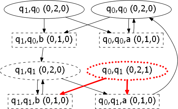
The first is from Fig. 6, in Section 2.4.1 we already saw that Spoiler can not win the game, no matter where the starting position is. Thus and because of Theorem 4 $q_{0}\preceq_{f}q_{1}$ and $q_{1}\preceq_{f}q_{0}$ . Hence we already know the correct result, after program termination every vertex must have a progress measure lower than infinity. We also know the amount of vertices with a priority of $1$ , it is $n=1$ . This means as soon as a the progress measure $\mu$ of a vertex $v$ that has $\mu(v)=1$ should be increased it reachs infinity.

Looking at Fig. 7 we see the game graph after the algorithm has terminated. In this example the program will only make one iteration and then terminate. First we notice the default values of a vertex, for best-nghb-ms it is $0$ , nghb-cnt is the amount of successors and $\mu$ also is $0$ . The vertex $(q_{0},q_{1})$ initially also had these default values, $(0,2,0)$ .

The working list of the algorithm is initialized with $(q_{0},q_{1})$ since this is the only vertex that has a priority of $1$ . In lines 6-22 the first iteration starts with $v=(q_{0},q_{1})$ now. In line 10 the best-nghb-ms of $v$ gets calculated based on its succeeding vertices. $v$ has a priority of $1$ and is in $V_{1}$ , this means it is Spoiler’s turn to make a move. Because of that he is looking for the successor with the highest progress measure, both successors have a progress measure of $0$ so any will be optimal. Therefore the best-nghb-ms of $v$ currently is $0$ and there are two successors having that measure, nghb-ms remains $2$ .

Line 12 updates the progress measure of $v$ based on its best-nghb-ms. Since the priority of $v$ is $1$ and the best-nghb-ms is $0$ the progress measure gets increased from $0$ to $1$ . The program now would inform the predecessors of $v$ about the update but since $v$ has no predecessors the iteration ends.

The working list is empty and the algorithm terminates. $(q_{0},q_{1})$ managed to increase its progress measure from $0$ to $1$ but not to $\infty$ , which would only be one additional update away. $(q_{0},q_{1})$ has a progress measure below $\infty$ thus $q_{1}\preceq_{f}q_{0}$ follows, analogously $q_{1}\preceq_{f}q_{0}$ follows from $(q_{1},q_{0})$ .

The basic concept is to update the data structures of a vertex based on its successors and then inform its predecessors about the update, maybe add them to the working list. If, for example, $q\not\preceq_{f}q^{\prime}$ then the algorithm will reversly build the path

	$\displaystyle\varrho=$	$\displaystyle\quad v_{0}\rightarrow v_{1}\rightarrow\ldots\rightarrow$
		$\displaystyle\quad\underbrace{v_{(q,q^{\prime})}\rightarrow\ldots\rightarrow pred(pred(v_{(q,q^{\prime})}))\rightarrow pred(v_{(q,q^{\prime})})\rightarrow v_{(q,q^{\prime})}}_{\text{loop}}\rightarrow\ldots$

by increasing the progress measure of $v_{(q,q^{\prime})}$ , adding a predecessor to the working list which also adds a predecessor to the working list and so on. This continues and $v_{(q,q^{\prime})}$ gets visited again through one of its successors, a loop is created, and it increases its progress measure again. The process repeats until the progress measure of $v_{(q,q^{\prime})}$ reaches $\infty$ , now all vertices on the loop also reach $\infty$ and the loop is completely processed.

This creates the path $\varrho$ reversly because we are informing predecessors. $v_{0},v_{1}\ldots$ may be vertices that are predecessors of a vertex that is involved in the loop. The created path has a lasso-type structure, first a chain of vertices and then a loop.

Next the second example which has more iterations.

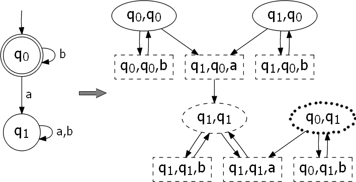
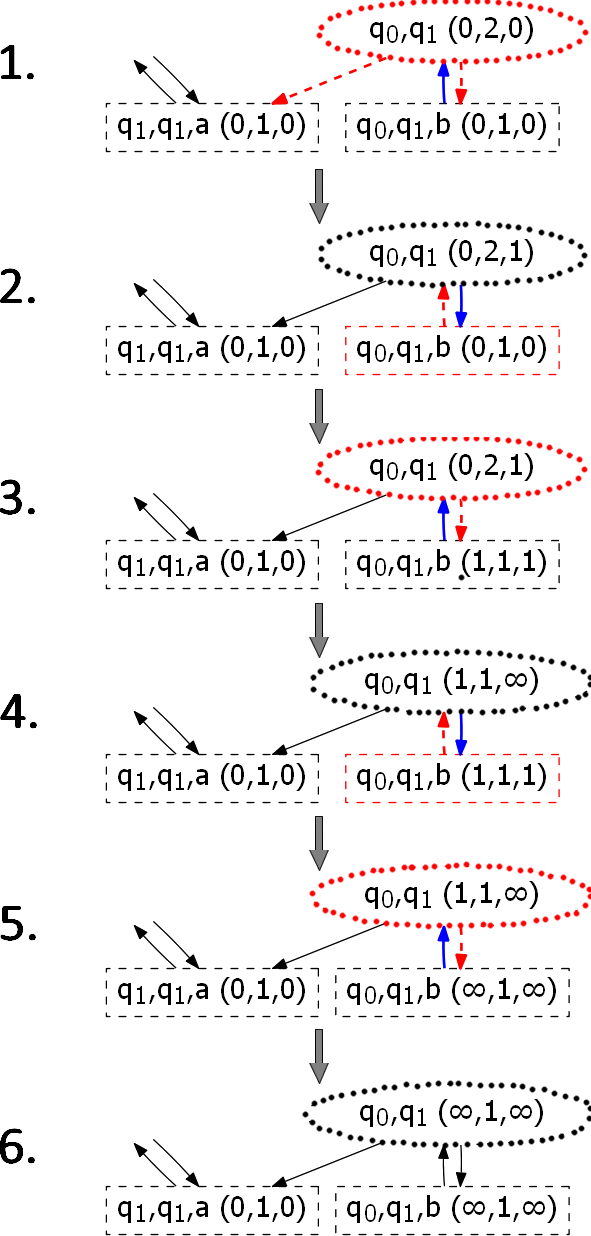
Fig. 8 shows an automaton with language $\{b^{\omega}\}$ . The language already tells that the two states can not be merged or the new language will be $\{(ab)^{\omega}\}$ . However, $q_{1}$ is of course redundant as it can not reach a final state. Note that the presented algorithm is not able to remove $q_{1}$ as it is not part of a mutually fair simulation.

In Fig. 9 the sequence of iterations the algorithm performs can be seen. $\infty$ comes after increasing beyond $n=1$ because there is only one vertex with a priority of $1$ . The working list gets initialized with $v=(q_{0},q_{1})$ , $v$ has two successors and both have the same progress measure, $0$ . Since $v$ has a priority of $1$ its progress measure gets increased to $1$ and lines 13-22 work through the predecessors of $v$ . There is only one predecessor, $w=(q_{0},q_{1},b)$ , and $w$ is in $V_{0}$ which means this vertex represents a move by Duplicator. Since Duplicator does not want to increase the progress measure of its vertices he seeks for another possibility to move at instead of $v$ . But $w$ has no better alternative, there is no other successor of $w$ with a smaller progress measure, the nghb-cnt of $w$ is $1$ . Therefore line 21 resolves to true and $w$ gets added to the working list.

In the second iteration the working vertex is $v=(q_{0},q_{1},b)$ . For $v$ the best-nghb-ms is the smallest progress measure of its successors since it is in $V_{0}$ . However, $v$ has only one successor, it has a progress measure of $1$ so $v$ must increase its progress measure to $2$ . We are again in lines 13-22 and work through the predecessors of $v$ . There is only $w=(q_{0},q_{1})\in V_{1}$ and line 16 resolves to true, $w$ is added to the working list.

This process repeats until $v=(q_{0},q_{1})$ reaches a progress measure of $\infty$ in the fourth iteration. It then again forces Duplicator’s vertex $w=(q_{0},q_{1},b)$ to be added into the working list. After the fifth iteration the cycle ends because line 15 resolves to false for $w$ . The reason why is that the progress measure of $v$ has not increased in this round, the best-nghb-ms of $w$ already is $\infty$ from the last iteration thus $\mu(v)\not>B(w)$ .

The program terminates because the working list is empty and we obtain two vertices with a progress measure of $\infty$ , $(q_{0},q_{1})$ and $(q_{0},q_{1},b)$ . We follow $q_{0}\not\preceq_{f}q_{1}$ but $q_{1}\preceq_{f}q_{0}$ since the vertex $(q_{1},q_{0})$ has a progress measure of $0$ .

Note that if $(q_{0},q_{1})$ would have another predecessor $u$ it would pass its $\infty$ , after creating the loop with $(q_{0},q_{1},b)$ , through $u$ . Of course this can only be the case if $u$ , which then would represent a move of Duplicator, has no better alternative to move at.

The third and last example demonstrates, the possibility of Duplicator to evade an update notification by choosing a better alternative.

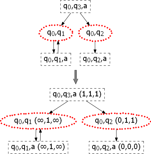
If we apply the algorithm to the game graph from Fig. 10 we initially have a working list of $\{(q_{0},q_{1}),(q_{0},q_{2})\}$ . We first work with $v=(q_{0},q_{2})$ which increases its progress measure to $1$ . Next $v$ notifies $w=(q_{0},q_{3},a)$ about its update but Duplicator has no interest in increasing the progress measure thus it chooses the vertex $(q_{0},q_{1})$ as a better successor than $v$ . This event corresponds to line 19, $w$ decreases its nghb-cnt to $1$ since it now only has one neighbor with its current optimal best-nghb-ms of $0$ and $w$ gets not added to the working list.

Next its $v=(q_{0},q_{1})$ turn and he also increases its progress measure to $1$ . Its predecessor $(q_{0},q_{1},a)$ gets added to the working list. The other predecessor $w=(q_{0},q_{3},a)$ now also gets added since both of its successors currently have a progress measure of $1$ . For $w$ there is no better alternative to move at as to $v$ or $(q_{0},q_{2})$ . This represents line 21 in the algorithm and the nghb-cnt of $w$ was previously decreased from $2$ to $1$ thus $w$ gets added to the working list.

Now working $(q_{0},q_{3},a)$ will increase its progress measure to $1$ , set its best-nghb-ms to $1$ and nghb-cnt to $2$ .

As next step working $(q_{0},q_{1},a)$ increases its progress measure and adds $(q_{0},q_{1})$ again which, when worked, increases its progress measure to $2$ . $v=(q_{0},q_{1})$ now tries to notify $w=(q_{0},q_{3},a)$ a second time to pass its progress measure of $2$ . Although line 18 resolves to true, since $v$ represented one of the optimal choices to move at in the last round, $w$ gets not added to the working list again because Duplicator better moves to $(q_{0},q_{2})$ . This is represented by line 19 and the nghb-cnt of $w$ gets decreased to $1$ again.

The vertex $v=(q_{0},q_{1})$ together with $(q_{0},q_{1},a)$ will create a loop and increase their progress measures to $\infty$ . In every iteration $v$ tries to notify $w=(q_{0},q_{3},a)$ about the update but the best-nghb-ms of $w$ is still only $1$ , representing $(q_{0},q_{2})$ as optimal choice, thus line 18 resolves to false (more precisely: $t\neq B(w)$ ) in every following iteration.

The program terminates after $v=(q_{0},q_{1})$ and $(q_{0},q_{1},a)$ have reached a progress measure of $\infty$ and they could not pass $\infty$ to $w=(q_{0},q_{3},a)$ . $w$ prefers to move to $(q_{0},q_{2})$ and accepts its progress measure of $1$ which is far better than $\infty$ for Duplicator.

4 Minimization using fair simulation

In this section we see how to reduce the size of a Büchi automaton using fair simulation. For this we use two techniques, the first allows us to merge pairs of states and the second technique removes transitions. First the chain of proof that connects merging and transition removal to fair simulation is constructed. After that we present the complete minimization algorithm.

In order to reduce the size of a Büchi automaton $A$ we need to modify it, merge states or remove transitions. Let $A^{\prime}$ be the automaton received after applying the desired modifications. We then evaluate if the language of the automaton did change. If it does not, $\mathcal{L}(A)=\mathcal{L}(A^{\prime})$ , the modifications are executed and $A:=A^{\prime}$ .

Merging of two states $q_{1}$ and $q_{2}$ is achieved by adding transitions and then removing one of the states from the automaton. Section 4.3 describes this process in detail.

Both of our techniques are achieved by adding or removing transitions and then checking if the language did change.

4.1 Language preservation

This section shows how fair simulation is used for merging two states and the removal of a transition such that it preserves the language.

Definition 21.

We define that two states $q$ and $q^{\prime}$ of a Büchi automaton $A=\langle\Sigma,Q,Q_{0},\Delta,F\rangle$ have the same in- and outgoing possibilities iff the following holds.

\displaystyle\begin{pmatrix}&\exists a\in\Sigma,q^{\prime}\in Q:(q_{1},a,q^{\prime})\in\Delta\Rightarrow\exists(q_{2},a,q^{\prime})\in\Delta\\ \land&\exists a\in\Sigma,q^{\prime}\in Q:(q^{\prime},a,q_{1})\in\Delta\Rightarrow\exists(q^{\prime},a,q_{2})\in\Delta\\ \land&\exists a\in\Sigma,q^{\prime}\in Q:(q_{2},a,q^{\prime})\in\Delta\Rightarrow\exists(q_{1},a,q^{\prime})\in\Delta\\ \land&\exists a\in\Sigma,q^{\prime}\in Q:(q^{\prime},a,q_{2})\in\Delta\Rightarrow\exists(q^{\prime},a,q_{1})\in\Delta\end{pmatrix}

Next we define the relation $\sim$ between states to hold iff both states have the same in- and outgoing possibilities.

Lemma 8.

Given two states $q_{1},q_{2}\in Q$ of a Büchi automaton $A=\\ \langle\Sigma,Q,Q_{0},\Delta,F\rangle$ where $A^{\prime}$ is the automaton obtained by removing $q_{2}$ (or $q_{1}$ if $q_{2}\in F\land q_{1}\notin F$ ) and all its in- and outgoing transitions, i.e. merging states $q_{1}$ and $q_{2}$ . the following holds.

\displaystyle q_{1}\sim q_{2}\Rightarrow\mathcal{L}(A)=\mathcal{L}(A^{\prime})

I.e. merging $q_{1}$ and $q_{2}$ does not change the language if they have the same in- and outgoing possibilities.

Proof.

We proof by contradiction, assuming $\mathcal{L}(A)\neq\mathcal{L}(A^{\prime})$ .

1.

$\mathcal{L}(A)\supset\mathcal{L}(A^{\prime})\Rightarrow\exists w=a_{1}a_{2}a_{3}\ldots:w\in\mathcal{L}(A)\land w\notin\mathcal{L}(A^{\prime})$
Let $\pi=q^{\prime}_{0}a_{1}q^{\prime}_{1}a_{2}q^{\prime}_{2}a_{3}q^{\prime}_{3}\ldots$ be an arbitrary run that corresponds to $w$ and $w.l.o.g.$ the states where merged by removing $q_{2}$ . We construct $\pi^{\prime}$ from $\pi$ by exchanging $q_{2}$ with $q_{1}$ . $\pi^{\prime}$ is still a valid run since if $\pi$ uses $(q^{\prime},a,q_{2})$ or $(q_{2},a,q^{\prime})$ it follows that the transition $(q^{\prime},a,q_{1})$ or $(q_{1},a,q^{\prime})$ does also exist by the left hand side of the lemma. But $q_{1}$ and its transitions do also exist in $A^{\prime}$ because we only removed $q_{2}$ . We follow that $\pi^{\prime}$ corresponds to $w$ , forms an accepting run and $w\in\mathcal{L}(A^{\prime})$ . ↯
2.

$\mathcal{L}(A)\subset\mathcal{L}(A^{\prime})\Rightarrow\exists w=a_{1}a_{2}a_{3}\ldots:w\notin\mathcal{L}(A)\land w\in\mathcal{L}(A^{\prime})$
Let $\pi^{\prime}=q^{\prime}_{0}a_{1}q^{\prime}_{1}a_{2}q^{\prime}_{2}a_{3}q^{\prime}_{3}\ldots$ be an arbitrary run that corresponds to $w$ and $w.l.o.g.$ the states where merged by removing $q_{2}$ . We immediately see that $\pi=\pi^{\prime}$ forms an accepting run in $A$ because every existing transition or state from $A^{\prime}$ also exists in $A$ . We follow that $w\in\mathcal{L}(A)$ . ↯

This follows $\mathcal{L}(A)=\mathcal{L}(A^{\prime})$ , the language did not change.
∎

Using Lemma 8 we can safely merge two states if both have the same in- and outgoing possibilities (Definition 21). But what if this is not the case? For example if there is a transition $(q_{1},a,q_{3})$ and the corresponding transition $(q_{2},a,q_{3})$ does not exist. We need to add $(q_{2},a,q_{3})$ to the automaton and check wether this changed the language. This is where the correlation to simulation shows.

So far fair simulation was only used for states from one automaton. If two automata $A$ and $A^{\prime}$ only differ in their set of transitions we now use fair simulation between two automata. For example $q\preceq_{f}q^{\prime}$ where $q$ is a state from $A$ and $q^{\prime}$ a state from $A^{\prime}$ . Recalling Definition 5, fair simulation is easily extended by letting the left hand side of the implications use transitions of $A$ and the right hand side transitions from $A^{\prime}$ .

Using this we define fair simulation between automata.

Definition 22.

Given two Büchi automata $A=\langle\Sigma,Q,Q_{0},\Delta,F\rangle$ and $A^{\prime}=\langle\Sigma,Q,Q^{\prime}_{0},\Delta^{\prime},F\rangle$ where $Q_{0}=Q^{\prime}_{0}$ we say

\displaystyle A^{\prime}\textnormal{ fairly simulates }A\text{ iff }\forall q\in Q_{0}\exists q^{\prime}\in Q^{\prime}_{0}:q\preceq_{f}q^{\prime}

Next we see how fair simulation between automata preserves language.

Colorally 2.

Given a Büchi automaton $A=\langle\Sigma,Q,Q_{0},\Delta,F\rangle$ and two states $q,q^{\prime}\in Q$ it holds that $q\preceq_{f}q^{\prime}\Rightarrow\mathcal{L}(A^{q})\subseteq\mathcal{L}(A^{q^{\prime}})$

Proof.

Follows directly from the definition of fair simulation as described in Definition 5.
∎

Lemma 9.

Given two Büchi automata $A=\langle\Sigma,Q,Q_{0},\Delta,F\rangle$ , $A^{\prime}=\\ \langle\Sigma,Q,Q_{0}^{\prime},\Delta^{\prime},F\rangle$ where $Q_{0}=Q_{0}^{\prime}$ , the following holds

\displaystyle A^{\prime}\text{ fairly simulates }A\Rightarrow\mathcal{L}(A)\subseteq\mathcal{L}(A^{\prime})

Proof.

Since $A^{\prime}$ fairly simulates $A$ we know that there exists a $q^{\prime}\in Q^{\prime}_{0}$ for each $q\in Q_{0}$ so that $q\preceq_{f}q^{\prime}$ . With Corollary 2 $\mathcal{L}(A^{q})\subseteq\mathcal{L}(A^{\prime q^{\prime}})$ follows.

\displaystyle\mathcal{L}(A)=\bigcup\limits_{q\in Q_{0}}\mathcal{L}(A^{q})\subseteq\bigcup\limits_{q^{\prime}\in Q^{\prime}_{0}}\mathcal{L}(A^{\prime q^{\prime}})=\mathcal{L}(A^{\prime}).

∎

Theorem 5.

$A=\langle\Sigma,Q,Q_{0},\Delta,F\rangle$ , $A^{\prime}=\langle\Sigma,Q,Q_{0}^{\prime},\Delta^{\prime},F\rangle$ are two Büchi automata and $Q_{0}=Q_{0}^{\prime}$ . Then, if both automata fairly simulate each other, their language is the same.

\displaystyle(A^{\prime}\text{ fairly simulates }A\land A\text{ fairly simulates }A^{\prime})\Rightarrow\mathcal{L}(A)=\mathcal{L}(A^{\prime})

Proof.

$\mathcal{L}(A)\subseteq\mathcal{L}(A^{\prime})\land\mathcal{L}(A)\supseteq\mathcal{L}(A^{\prime})\Rightarrow\mathcal{L}(A)=\mathcal{L}(A^{\prime})$ . Using Lemma 9 we are done.
∎

For language equality we need inclusion in both directions, $\mathcal{L}(A)\subseteq\mathcal{L}(A^{\prime})$ and $\mathcal{L}(A)\supseteq\mathcal{L}(A^{\prime})$ . So if we add transitions for an attempted merge we need to check if $A$ fairly simulates $A^{\prime}$ and if also $A^{\prime}$ fairly simulates $A$ . The same applies if we want to remove transitions, language does not change if we have fair simulation in both directions between the automaton before and after the modification.

4.2 Modifing the game graph

For checking language inclusion we use a method that allows us to efficiently modify the game graph.

We present tools for game graph manipulation and in the next section take a closer look on how they are used to compute language inclusion.

Definition 23.

For a given Büchi automaton $A=\langle\Sigma,Q,Q_{0},\Delta,F\rangle$ , a game graph $G^{f}_{A,A^{\prime}}=\langle V_{0},V_{1},E,p\rangle$ and a set of transitions $T\subseteq Q\times\Sigma\times Q$ , we make the following four definitions.

1.

$\textnormal{rem}(A,T)=\langle\Sigma,Q,Q_{0},\Delta\setminus T,F\rangle$ is the automaton without transitions in $T$ .
2.

$\textnormal{rem}(G^{f}_{A,A^{\prime}},T)$ is the game graph $\langle V_{0},V_{1},E^{\prime},p\rangle$ where

$E^{\prime}=E\setminus\{\underbrace{\left(v_{(q,q^{\prime},a)},v_{(q,\tilde{q})}\right)}_{\text{transition of Duplicator}}|v_{(q,q^{\prime},a)}\in V_{0},v_{(q,\tilde{q})}\in V_{1},$

$(q^{\prime},a,\tilde{q})\in T\}$ .
3.

$\textnormal{add}(A,T)=\langle\Sigma,Q,Q_{0},\Delta\cup T,F\rangle$ is the automaton $A$ additionally with transitions in $T$ .
4.

$\textnormal{add}(G^{f}_{A,A^{\prime}},T)$ is the game graph $\langle V_{0},V_{1},E^{\prime},p\rangle$ where

$E^{\prime}=E\cup\{\underbrace{\left(v_{(q,q^{\prime})},v_{(\tilde{q},q^{\prime},a)}\right)}_{\text{transition for Spoiler}}|v_{(q,q^{\prime})}\in V_{1},$

$v_{(\tilde{q},q^{\prime},a)}\in V_{0},(q,a,\tilde{q})\in T\}$ .

As we see rem removes transitions, given as set $T$ , only from Duplicator’s automaton and add adds transitions only to Spoiler’s automaton.

Lemma 10.

Given two given Büchi automaton $A=\langle\Sigma,Q,Q_{0},\Delta,F\rangle$ and $A^{\prime}=\langle\Sigma,Q,Q_{0},\Delta^{\prime},F\rangle$ , where $T$ is a set of transitions. If $\Delta^{\prime}=\Delta\setminus T$ then $G^{f}_{A,A^{\prime}}=\textnormal{rem}(G^{f}_{A,A},T)$ . If $\Delta^{\prime}=\Delta\cup T$ then $G^{f}_{A^{\prime},A}=\textnormal{add}(G^{f}_{A,A},T)$ .

Proof.

Since $\text{add}(A,T)=A^{\prime}$ we directly follow that the game graph constructed by $G^{f}_{A^{\prime},A}$ is the same as that generated by modifying $G^{f}_{A,A}$ by using $\text{add}(G^{f}_{A,A},T)$ . This is because add only adds transitions to Spoiler, the same transitions that would be generated by giving Spoiler the automaton $A^{\prime}$ for use from beginning.

Analogue for rem where Duplicator looses the same transitions that would be left if he directly started with the modified automaton $A^{\prime}$ .
∎

Colorally 3.

Furthermore, given two Büchi automata $A$ , $A^{\prime}$ and two sets of transitions $T$ , $T^{\prime}$ , we have

1.

$G^{f}_{A,\textnormal{rem}(A,T)}=\textnormal{rem}(G^{f}_{A,A},T)$ and

$\textnormal{rem}(\textnormal{rem}(G^{f}_{A,A},T),T^{\prime})=\textnormal{rem}(G^{f}_{A,A},T\cup T^{\prime})$ .
2.

$G^{f}_{\textnormal{add}(A,T),A}=\textnormal{add}(G^{f}_{A,A},T)$ and

$\textnormal{add}(\textnormal{add}(G^{f}_{A,A},T),T^{\prime})=\textnormal{add}(G^{f}_{A,A},T\cup T^{\prime})$ .

Proof.

Directly follows from Lemma 10.
∎

4.3 Merge states

We have seen that a pair of states $(q,q^{\prime})$ can be merged without changing the language of the automaton when they directly or delayedly simulate each other. For fair simulation this is not the case. However, chances are high in practice that such a pair can also be merged without changing the language. We say $(q,q^{\prime})$ is of interest for merging if the states fairly simulate each other,

\displaystyle q\preceq_{f}q^{\prime}\land q^{\prime}\preceq_{f}q.

Given such a pair we construct the automaton $A^{\prime}$ where both states have the same in- and outgoing possibilites, i.e. $q\sim q^{\prime}$ (Definition 21).

In detail we define $A^{\prime}$ as the automaton $add(A,T)$ where

	$\displaystyle T=\{(q,a,\tilde{q})\notin\Delta\|(q^{\prime},a,\tilde{q})\in\Delta\}$
	$\displaystyle\cup\{(\tilde{q},a,q)\notin\Delta\|(\tilde{q},a,q^{\prime})\in\Delta\}$
	$\displaystyle\cup\{(q^{\prime},a,\tilde{q})\notin\Delta\|(q,a,\tilde{q})\in\Delta\}$
	$\displaystyle\cup\{(\tilde{q},a,q^{\prime})\notin\Delta\|(\tilde{q},a,q)\in\Delta\}$	.

Recalling Theorem 5 we need to compute if $A^{\prime}$ fairly simulates $A$ and if $A$ fairly simulates $A^{\prime}$ .

The first computation is easy. We already know that $A^{\prime}$ fairly simulates $A$ because $A^{\prime}$ has more transitions than $A$ . Hence it intuitively has more possibilities.

For $A^{\prime}$ to fairly simulate $A$ we need to show $\forall q\in Q_{0}\exists q^{\prime}\in Q^{\prime}_{0}:q\preceq_{f}q^{\prime}$ . We simply select $q^{\prime}=q$ and $q\preceq_{f}q^{\prime}$ holds because if $q$ in $A$ builds an accepting run $\pi$ then $q^{\prime}$ in $A^{\prime}$ can build the same run $\pi^{\prime}=\pi$ . All transitions from $A$ are also available for $q^{\prime}$ in $A^{\prime}$ .

The second computation is not trivial, to compute if $A$ fairly simulates $A^{\prime}$ we construct the game graph $G^{f}_{A^{\prime},A}=add(G^{f}_{A},T)$ . This is the game graph where Spoiler plays on $A^{\prime}$ and Duplicator on $A$ .

Theorem 6.

Let $\mu$ be the progress measure function obtained by applying Algorithm 1 to the graph without modifications $G^{f}_{A}$ .

Also let $\mu^{\prime}$ be the progress measure function obtained by applying the algorithm to the modified game graph $\text{add}(G^{f}_{A},T)=G^{f}_{A^{\prime},A}$ , where $T$ is a set of transitions. Then the following holds.

	$\displaystyle A\text{ fairly simulates }A^{\prime}\text{ iff }\forall v\in V:(\mu(v)\neq\infty\Rightarrow\mu^{\prime}(v)\neq\infty)$
	$\displaystyle\land(\mu(v)=\infty\Rightarrow\mu^{\prime}(v)=\infty)$

Proof.

If the right hand side holds we directly follow

\displaystyle\forall q^{\prime}\in Q^{\prime}_{0}\exists q\in Q_{0}:q^{\prime}\preceq_{f}q\overset{\textbf{Definition\penalty\ \ref{def_automatasimulation}}}{\Longrightarrow}A\text{ fairly simulates }A^{\prime}

since we trivially have $q_{i}\preceq_{f}q_{i}\forall i$ in $G^{f}_{A}$ and also in $G^{f}_{A^{\prime},A}$ , we simply select $q=q^{\prime}$ .

If $A$ fairly simulates $A^{\prime}$ we have $\forall q^{\prime}\in Q^{\prime}_{0}\exists q\in Q_{0}:q^{\prime}\preceq_{f}q$ , i.e. the trivial pairs $q^{\prime}_{i}\preceq_{f}q_{i}$ where $q^{\prime}_{i}=q_{i}$ . Since $\preceq_{f}$ transitive, which easily can be seen, we build all other elements $\tilde{q}\preceq_{f}q_{i}$ of the simulation relation with $\tilde{q}\preceq_{f}q^{\prime}_{i}$ by using

\displaystyle\tilde{q}\preceq_{f}q^{\prime}_{i}\land q^{\prime}_{i}\preceq_{f}q_{i}\Rightarrow\tilde{q}\preceq_{f}q_{i}.

∎

We see that if we apply Algorithm 1 to $G^{f}_{A^{\prime},A}$ and the obtained simulation relation is the same as after running the algorithm on $G^{f}_{A}$ , $A$ fairly simulates $A^{\prime}$ . Together with the trivial statement that $A^{\prime}$ fairly simulates $A$ we receive language equivalence $\mathcal{L}(A)=\mathcal{L}(A^{\prime})$ by Theorem 5. Both states then have the same in- and outgoing possibilities, we apply Lemma 8 and merge the two states without changing the language.

Summarized we first search for pairs $(q,q^{\prime})$ where $q\preceq_{f}q^{\prime}$ and $q^{\prime}\preceq_{f}q$ . Then we construct $G^{f}_{A^{\prime},A}$ and run Algorithm 1 on it. We compare results and if both simulation relations are equal the merge is accepted and does not change the language of the automaton.

4.4 Remove redundant transitions

A transition $(q,a,q^{\prime})$ is of interest for removal if

\displaystyle\exists\tilde{q}\in Q:(q,a,\tilde{q})\in\Delta\land q^{\prime}\preceq_{f}\tilde{q}.

In practice chances are high that such transitions do not change the language when removed, compared to arbitrary transitions. Given such a transition we construct the automaton $A^{\prime}$ where this transition was removed. In detail $A^{\prime}=rem(G^{f}_{A},T)$ where $T=\{(q,a,q^{\prime})\}$ .

We again recall Theorem 5 and compute if $A^{\prime}$ fairly simulates $A$ and $A$ fairly simulates $A^{\prime}$ .

This time the second computation is easy. If we remove transitions from $A$ we already know that $A$ fairly simulates the received automaton $A^{\prime}$ because $A^{\prime}$ intuitively has less possibilities.

For $A$ to fairly simulate $A^{\prime}$ we need to show $\forall q^{\prime}\in Q^{\prime}_{0}\exists q\in Q_{0}:q^{\prime}\preceq_{f}q$ . We select $q=q^{\prime}$ and $q^{\prime}\preceq_{f}q$ holds because if $q^{\prime}$ in $A^{\prime}$ builds an accepting run $\pi^{\prime}$ then $q$ in $A$ can build the same path $\pi=\pi^{\prime}$ . All transitions from $A^{\prime}$ are also available for $q$ in $A$ , i.e. for all transitions $(q^{\prime},a,\tilde{q})$ in $A^{\prime}$ there does also exist the transition $(q,a,\tilde{q})$ in $A$ , analogously for transitions $(\tilde{q},a,q^{\prime})$ in $A^{\prime}$ there exists the transition $(\tilde{q},a,q)$ in $A$ .

The first computation is not trivial, we proceed likewise to Section 4.3. In order to compute if $A^{\prime}$ fairly simulates $A$ , we consruct the game graph $G^{f}_{A,A^{\prime}}=rem(G^{f}_{A},T)$ . In this game graph Spoiler plays on $A$ and Duplicator on the modified automaton $A^{\prime}$ .

Theorem 7.

Let $\mu$ be the progress measure function obtained by applying Algorithm 1 to the graph without modifications $G^{f}_{A}$ .

Also let $\mu^{\prime}$ be the progress measure function obtained by applying the algorithm to the modified game graph $\text{rem}(G^{f}_{A},T)=G^{f}_{A,A^{\prime}}$ , where $T$ is a set of transitions. Then the following holds.

	$\displaystyle A^{\prime}\text{ fairly simulates }A\text{ iff }\forall v\in V:(\mu^{\prime}(v)\neq\infty\Rightarrow\mu(v)\neq\infty)$
	$\displaystyle\land(\mu^{\prime}(v)=\infty\Rightarrow\mu(v)=\infty)$

Proof.

Analogously as for Theorem 6.
∎

If both simulation relations are the same we receive that $A^{\prime}$ fairly simulates $A$ , together with $A$ fairly simulates $A^{\prime}$ we now obtain language equivalence, $\mathcal{L}(A)=\mathcal{L}(A^{\prime})$ for removing the transition.

Summarized we first search for transitions of interest $(q,a,q^{\prime})$ . Then we construct $G^{f}_{A,A^{\prime}}$ and run Algorithm 1 on it. We compare results and if both simulation relations are equal the transition removal is accepted and does not change the language of the automaton.

4.5 Algorithm

Take a look at Algorithm 3, first presented in [7], the complete minimization algorithm that uses the introduced techniques to reduce the size of a Büchi automaton using fair simulation.

Algorithm 3 Complete algorithm for minimization of Büchi automaton

A=\langle\Sigma,Q,Q_{0},\Delta,F\rangle

using fair simulation.

G^{f}_{\textnormal{{A}}}:=\langle V_{0},V_{1},E,p\rangle

;

\textnormal{{V}}:=V_{0}\cup V_{1}

;

\textnormal{{$\mu$}}:=\textbf{Algorithm\penalty\ \ref{algo_jurdzinski}}(G^{f}_{\textnormal{{A}}})

;

\textnormal{{L}}_{1}:=\emptyset

;

5 for $\textnormal{{v}}_{(q,q^{\prime})}\in\textnormal{{V}}:\mu(\textnormal{{v}}_{(q,q^{\prime})})<\infty$ do

6 if $\textnormal{{$\mu$}}(\textnormal{{v}}_{(q^{\prime},q)})<\infty\land\textnormal{{v}}_{(q^{\prime},q)}\notin\textnormal{{L}}_{1}$ then

\textnormal{{L}}_{1}:=\textnormal{{L}}_{1}\cup\textnormal{{v}}_{(q,q^{\prime})}

;

\textnormal{{L}}_{2}:=\emptyset

;

9 for $(q,a,q^{\prime})\in\Delta:\left(\exists\tilde{q}\in Q:(q,a,\tilde{q})\in\Delta\land\textnormal{{$\mu$}}(\textnormal{{v}}_{(q^{\prime},\tilde{q})})<\infty\right)$ do

\textnormal{{L}}_{2}:=\textnormal{{L}}_{2}\cup(q,a,q^{\prime})

;

\textnormal{{S}}_{1}:=\emptyset

;

12 for $\textnormal{{v}}_{(q,q^{\prime})}\in\textnormal{{L}}_{1}$ do

\textnormal{{T}}:=\{(q,a,\tilde{q})\notin\Delta|(q^{\prime},a,\tilde{q})\in\Delta\}

;

\cup\{(\tilde{q},a,q)\notin\Delta|(\tilde{q},a,q^{\prime})\in\Delta\}

;

\cup\{(q^{\prime},a,\tilde{q})\notin\Delta|(q,a,\tilde{q})\in\Delta\}

;

\cup\{(\tilde{q},a,q^{\prime})\notin\Delta|(\tilde{q},a,q)\in\Delta\}

;

\textnormal{{$\mu$}}^{\prime}:=\textbf{Algorithm\penalty\ \ref{algo_jurdzinski}}(\textnormal{{add}}(G^{f}_{\textnormal{{A}}},\textnormal{{T}}))

;

18 if $\forall\textnormal{{v}}\in\textnormal{{V}}:\left(\textnormal{{$\mu$}}^{\prime}(\textnormal{{v}})\neq\infty\Rightarrow\textnormal{{$\mu$}}(\textnormal{{v}})\neq\infty\right)\newline \qquad\qquad\land\left(\textnormal{{$\mu$}}^{\prime}(\textnormal{{v}})=\infty\Rightarrow\textnormal{{$\mu$}}(\textnormal{{v}})=\infty\right)$ then

\textnormal{{S}}_{1}:=\textnormal{{S}}_{1}\cup\textnormal{{v}}_{(q,q^{\prime})}

;

\textnormal{{S}}_{2}:=\emptyset

;

21 for $(q,a,q^{\prime})\in\textnormal{{L}}_{2}$ do

\textnormal{{T}}:=\{(q,a,q^{\prime})\}

;

\textnormal{{$\mu$}}^{\prime}:=\textbf{Algorithm\penalty\ \ref{algo_jurdzinski}}(\textnormal{{rem}}(G^{f}_{\textnormal{{A}}},\textnormal{{T}}))

;

24 if $\forall\textnormal{{v}}\in\textnormal{{V}}:\left(\textnormal{{$\mu$}}^{\prime}(\textnormal{{v}})\neq\infty\Rightarrow\textnormal{{$\mu$}}(\textnormal{{v}})\neq\infty\right)\newline \qquad\qquad\land\left(\textnormal{{$\mu$}}^{\prime}(\textnormal{{v}})=\infty\Rightarrow\textnormal{{$\mu$}}(\textnormal{{v}})=\infty\right)$ then

\textnormal{{S}}_{2}:=\textnormal{{S}}_{2}\cup(q,a,q^{\prime})

;

26 for $\textnormal{{v}}_{(q,q^{\prime})}\in\textnormal{{S}}_{1}$ do

27 A:=

\textnormal{{merge}}(q,q^{\prime},\textnormal{{A}})

;

28 for $(q,a,q^{\prime})\in\textnormal{{S}}_{2}$ do

29 A:=

\textnormal{{remove}}((q,a,q^{\prime}),\textnormal{{A}})

;

30 return A;

Lines 1-3 construct the game graph and apply the initial run of Algorithm 1.

In lines 4-10 we compute the states of interest for merging and store it in $L_{1}$ . We store the transitions of interest for removal in $L_{2}$ . As specified in Section 4.3 and Section 4.4.

Lines 11-25 check if merging or transition removal would change the language of the automaton. If a merge would not change the language the pair gets stored in $S_{1}$ , and $S_{2}$ stores the transitions that would not change the language if removed. In lines 13-16 the set $T$ describes the transitions that need to be added for $q$ and $q^{\prime}$ to have the same in- and outgoing possibilities as seen in Section 4.3. Line 18 and 24 represent Theorem 6 and Theorem 7 respectively.

Lines 26-29 merge pairs of states and remove transitions that do not change the language if merged or removed.

4.5.1 Complexity

Before we start to analyze the complexity of the minimization algorithm let us establish some assumptions. We assume that checking the conditions in lines 5, 6, 9, 18, 24 can be done in constant time. Most of them can be checked while proccessing Algorithm 1 and, for example, $L_{1}$ can be implemented as Hashset which allows membership test in constant time.

Also we assume that we only hold one game graph in the memory. If we need to change the game graph, in lines 17, 23, we do not create a new game graph and instead modify the original graph. If the modification changes the language we undo the changes, this is described in Section 5 in more detail.

Theorem 8.

Given a Büchi automaton $A=\langle\Sigma,Q,Q_{0},\Delta,F\rangle$ Algorithm 3 runs in $\mathcal{O}(|Q|^{4}\cdot|\Delta|^{2})$ time and $\mathcal{O}(|Q|\cdot|\Delta|)$ space.

Proof.

Let us first analyze the space complexity. Theorem 1 states that Algorithm 1 runs in $\mathcal{O}(|Q|\cdot|\Delta|)$ space. But we first need to construct the game graph and hold it in memory. However, the game graph also has a size of $|Q|\cdot|\Delta|$ as we know from Lemma 4. It will not increase the space complexity.

Lists $L_{1},L_{2},S_{1},S_{2}$ store vertices and transitions which are of interest. Their size depends on the size of the game graph, $|Q|\cdot|\Delta|$ . The progress measure function $\mu$ needs to be holded in memory the whole time. Its domain is $V$ , the vertices of the game graph, but $|V|\in\mathcal{O}(|Q|\cdot|\Delta|)$ . So in total we have a space complexity of $\mathcal{O}(|Q|\cdot|\Delta|)$ .

For the time complexity we first spot Algorithm 1 runs in $\mathcal{O}(|Q|^{3}\cdot|\Delta|)$ time as Theorem 1 states.

For constructing the initial game graph $G^{f}_{A}$ we need to iterate over each state and each transition especially to create vertices $v_{(q,q^{\prime},a)}\in V_{0}$ . Therefore we have a time complexity of $\mathcal{O}(|Q|\cdot|\Delta|)$ for line 1.

Last we need to know how often we apply Algorithm 1 in lines 17, 23, let us refer with $k$ to this amount. Obviously $k$ is proportional to the number of attempted merges and transition removals. Those are dependent on the amount of simulation relation elements $\preceq_{f}$ and transitions $\Delta$ . Since $\preceq_{f}:Q\times Q$ we follow $k\in\mathcal{O}(|Q|^{2}+|\Delta|)\subseteq\mathcal{O}(2\cdot|Q|\cdot|\Delta|)$ because $|Q|^{2}\leq|Q|\cdot|\Delta|\land\Delta\leq|Q|\cdot|\Delta|$ as we know by Lemma 4.

In total we have a time complexity of $\mathcal{O}(|Q|^{3}\cdot|\Delta|\cdot k)\subseteq\mathcal{O}(|Q|^{4}\cdot|\Delta|^{2})$ .
∎

4.6 Examples

Let us consider two examples. The first example is the automaton of Fig. 2. We see its game graph after the initial run of Algorithm 1 in Fig. 7. The algorithm yields $q_{0}\preceq_{f}q_{1}$ and $q_{1}\preceq_{f}q_{0}$ so this pair is of interest for merging.

Next we need to compute $T$ , the set of transitions that need to be added for $q_{0}$ and $q_{1}$ to have the same in- and outgoing possibilities. $q_{0}$ has predecessors $q_{0}$ and $q_{1}$ both with letter $a$ . $q_{1}$ now also needs this predecessors, we add $(q_{0},a,q_{1})$ and $(q_{1},a,q_{1})$ to $T$ . $q_{0}$ has successors $q_{0}$ , with $a$ , and $q_{1}$ , with $b$ . $q_{1}$ already has both required transitions. Now we move to $q_{1}$ , it has two predecessors $q_{0}$ and $q_{1}$ both with letter $b$ , we need to add $(q_{0},b,q_{0})$ and $(q_{1},b,q_{0})$ to $T$ . Since $q_{0}$ already has all transitions required by the successors of $q_{1}$ we are done and

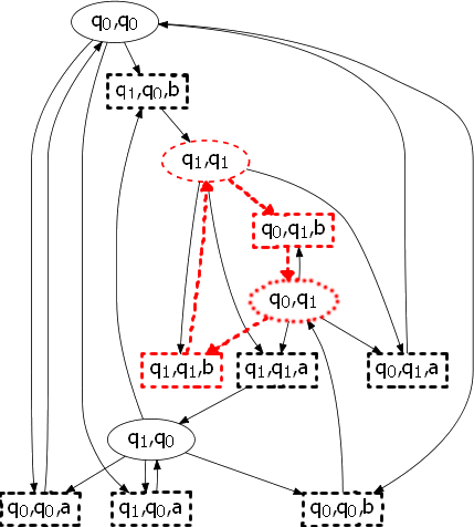
\displaystyle T=\{(q_{0},a,q_{1}),(q_{1},a,q_{1}),(q_{0},b,q_{0}),(q_{1},b,q_{0})\}.

Using $add(G^{f}_{A},T)$ creates the game graph seen in Fig. 11. When running Algorithm 1 on the modified game graph every vertex reaches a progress measure of $\infty$ . The resulting simulation relation $\preceq_{f}$ has no elements, there is no fair simulation anymore. By Theorem 6 we know this means the language changes if we merge $q_{0}$ and $q_{1}$ .

Algorithm 3 does not accept the attempted merge. Since there are no more merge candidates and no candidates for transition removal the program terminates.

In the next example we see the successful removal of a transition.

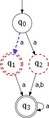
Looking at Fig. 12 we have an automaton with $q_{1}\preceq_{f}q_{2}$ , $q_{3}\preceq_{f}q_{0}$ and $q_{3}\preceq_{f}q_{2}$ which clearly can be seen. Although there is no pair of states for merging we can remove a transition.

In line 9 of Algorithm 3 we find the transition $(q_{0},a,q_{1})$ since there does exist transition $(q_{0},a,q_{2})$ and $q_{1}\preceq_{f}q_{2}$ . When building the game graph $rem(G^{f}_{A},\{(q_{0},a,q_{1})\})$ in line 23 we remove the edges

\displaystyle(v_{(q_{1},q_{0},a)},v_{(q_{1},q_{1})}),(v_{(q_{2},q_{0},a)},v_{(q_{2},q_{1})})\text{ and }(v_{(q_{3},q_{0},a)},v_{(q_{3},q_{1})})

from the original graph $G^{f}_{A}$ . As we see those edges are exactly the edges of Duplicator that would use the removed transition $(q_{0},a,q_{1})$ .

If we now apply Algorithm 1 on the modified game graph the resulting simulation relation is the same as before. By Theorem 7 this means the language does not change if $(q_{0},a,q_{1})$ is removed from the automaton. The attempted removal is accepted and the program terminates.

5 Optimization

This section presents some optimizations for the algorithm.

Reuse

When using Algorithm 1 in line 3 of Algorithm 3 in order to compute the simulation relation, we can reuse information for future runs of the algorithm in lines 17, 23. In practice modifcations on the game graph are small and most progress measures of vertices will not change.

Instead of initializing the progress measure of vertices or the arrays $B$ and $C$ with the default assignment, we can reuse information gathered from the first run of Algorithm 1 in line 3. The following lemma examines this more closely.

Lemma 11.

For the progress measures functions $\mu$ and $\mu^{\prime}$ received from $G^{f}_{A}$ and $\text{add}(G^{f}_{A},T)$ , where $T$ is a set of transitions, the following holds.

\displaystyle\forall v\in V:\mu(v)\leq\mu^{\prime}(v)

The same applies to $\text{rem}(G^{f}_{A},T)$ . I.e. the progress measure can only get greater after modifying the graph.

Proof.

The only changes made to the game graph were adding transitions to vertices $v\in V_{1}$ that belong to Spoiler. Since Spoiler always chooses a successor that increases the progress measure, if possible, the modification can only increase the progress measure of a vertex. This is because Spoiler has more possibilities to choose from after the modification.

If the progress measure is unchanged the modification did not give Spoiler a better choice than before, if it increased it did create a better choice.

Analogue for $\text{rem}(G^{f}_{A},T)$ were Duplicator can only loose and not gain opportunities to decrease the measure. The functions add and rem make the game harder to win for Duplicator.
∎

Lemma 11 allows us to initialize the data structures of every following run of Algorithm 1 with the values they had in the end of the first run. This can be done because we already know that Spoiler is capable of progressing to this progress measures. It can only happen that he progresses further. By doing so we reduce the running time by the part where the algorithm progresses to this state of progress measure.

In combination with the optimization game graph history we are even able to reuse the information gathered from the last successful modification instead only from the initial run of Algorithm 1.

However, we need to take a closer look on the working list of the algorithm. Normally it gets initialized with vertices which have a priority of $1$ but it can happen that we miss parts of the game graph. The modification, for example adding transitions, may lead to the creation of new vertices $v\in V_{0}$ in the game graph. Imagine the addition of transition $(q,a,q^{\prime})$ , this may create vertices $v_{(q,\tilde{q},a)}$ if there was no from $q$ outgoing transition labeled with $a$ before. If such a newly created vertex has a priority not equal to $0$ we also need to add it to the working list.

Preprocessing

A requirement of Algorithm 1 is that the input automaton neither has dead ends. Since they do not contribute to the language of the automaton we safely remove them before applying the algorithm by a linear search.

Furthermore this observation allows us to remove non live states [18] that do not contribute to the language of a Büchi automaton too.

Definition 24.

Given a Büchi automaton $A$ a state $q$ is live iff

\displaystyle\exists w\in\mathcal{L}(A)\exists\text{ corresponding run }\pi:q\in\pi

else $q$ is called a non live state. I.e. $q$ occurs in an accepting run on some word.

By doing so we reduce the size of the Büchi automaton and so the size of the game graph which often is a bottleneck.

Depending on the type of input automaton removing non live states may not always be a good idea, especially when the costs for removing them is greater than the benefit of a smaller game graph.

Fair-direct simulation

Merging two states $q,q^{\prime}$ is always possible without changing the language if they directly simulate each other (see [6]). This also applies to delayed simulation.

The idea for this optimization is to use delayed or direct simulation prior to fair simulation. Although delayed simulation, in contrast to direct simulation, yields more merge-equivalent pairs, the costs for creating the huge game graph are high. However, the game graph for direct simulation can be generated out of the graph for fair simulation by omitting some edges, as seen in Definition 9.

We generate the game graph for fair simulation $G^{f}_{A}$ and mark the edges needed to omit for a direct game graph. Then we easily transform it to a direct game graph $G^{di}_{A}$ , the costs for the transformation are in $\mathcal{O}(1)$ . Next we apply direct simulation by using $\textbf{Algorithm\penalty\ \ref{algo_jurdzinski}}(G^{di}_{A})$ and receive the relation $\preceq_{di}$ . After that we transform the graph back to $G^{f}_{A}$ , again the costs are in $\mathcal{O}(1)$ only. Now we start Algorithm 3. As we reach line 12, where we check if we can merge the states $q$ and $q^{\prime}$ without changing the language, we first check if they directly simulate each other, i.e. $q\preceq_{di}q^{\prime}\land q^{\prime}\preceq_{di}q$ . If that is the case, we already know that merging them does not change the language. We skip applying an additional run of Algorithm 1 and directly add the pair to $S_{1}$ .

We can do likewise for transition removal. It holds that a transition of interest for removal $(q,a,q^{\prime})$ can safely be removed without changing the language if $\exists\tilde{q}\in Q:(q,a,\tilde{q})\in\Delta\land q^{\prime}\preceq_{di}\tilde{q}$ , compare to Section 4.4. I.e. if the required relation is direct simulation, this was proven in [7].

This optimization is more useful if more pairs of directly simulating vertices exist.

Strongly connected components

As we have seen Algorithm 1 computes a bound, denoted by $\infty$ , for the progress measure. When a vertex reaches this bound one can be sure that there does not exist a winning strategy for Duplicator when starting at this vertex.

Normally this bound is set to $n+1$ where $n$ is the amount of vertices with a priority of $1$ . When increasing to a progress measure of $n+1$ we have visited $n+1$ vertices with priority $1$ without visiting priority $0$ . Then we are visiting at least one vertex with priority $1$ more than only once.

However, we can improve that bound for vertices locally. If, for example, we already know that a vertex can only reach $5$ vertices with priority $1$ where there are $30$ in total, why not setting the local bound for this vertex to $6$ instead of $31$ . The computation for vertices would finish much faster in many applications.

This is where we use strongly connected components, shortened to SCCs, lets take a look at the following definition.

Definition 25.

A SCC is a directed graph $G_{S}=\langle V,E\rangle$ , where $V$ is the set of vertices and $E$ the set of edges, that is strongly connected. $G_{S}$ is strongly connected iff

\displaystyle\forall v\in V\forall v^{\prime}\in V:v\text{ reachable from }v^{\prime},

i.e. every vertex in the SCC can be reached from every other vertex.

We can use algorithms that work in linear time, for example Tarjan’s algorithm [16], to compute every SCC of our game graph $G^{f}_{A}$ before we apply Algorithm 1. Now we compute for every vertex the local optimal bound which is the number of vertices with priority $1$ that are in the SCC. Next we can use Algorithm 1 on each SCC separately.

However, the SCCs need to propagate progress measure updates among themselves.

As Algorithm 3 uses Algorithm 1 multiple times while modifing the game graph and therefore calculating the SCCs each time from scratch we may reuse information. Since the game graph gets only slightly changed, we may already know how the SCCs change. If adding edges between SCCs they may merge to one SCC, if removing edges in a SCC it may split into several SCCs.

We can either disable the SCC optimization on following runs of Algorithm 1 and only use it on the first run or we maintain SCCs of SCCs, i.e. calculating which SCCs can be reached from other SCCs. If we have a SCC that contains several SCCs, we can merge them to one SCC. As there are far less SCCs than vertices in the game graph, the SCC calculation of SCCs may be fast, dependent on the type of input automaton.

Order of vertex processing

Algorithm 1 maintains the working list $L$ , it contains vertices that need to be processed by the algorithm. We can speed up the program by optimizing the order vertices get processed. The algorithm obviously terminates the fastest if all vertices reach a progress measure of $\infty$ as fast as possible, if they can. Therefore implementing the working list with a priority queue that first processes vertices with a higher progress measure will significantly speed up the process.

If we detect that vertices frequently get added to the working list we should prioritize them over others since chances are high they are part of a smaller loop which increases the progress measure faster to $\infty$ than bigger loops.

Game graph history

When implementing line 17, 23 of Algorithm 3 we should modify the original game graph instead of creating a new game graph, since their size is big. However, if an attempted merge or transition removal changes the language, we must be able to revert changes to the game graph. Making a backup of the original graph may not be a good idea, since they consume much space. But we can also memorize made changes and implement an undo method.

Note that when using the optimization reuse, we must also be able to revert changes to the data structures of Algorithm 1 before reusing them in future runs of the algorithm. Creating backups of the data structures needs space in the size of the game graph, $\mathcal{O}(|V|)$ . We should only memorize the exact changes that where made. For many vertices their value in the data structures will remain unchanged since the game graph gets only slightly modified.

When a modifcation does not change the language we keep the modified graph and use this graph for next modifications. This may slightly fasten the detection of future failing modifications, since the progress measure of vertices may be greater than in the unmodified game graph and reach $\infty$ faster.

Smart initialization

When applying Algorithm 1 to a game graph we may already know that a state $q^{\prime}$ does not fairly simulate $q$ . We then know for the vertex $v_{(q,q^{\prime})}$ or $v_{(q,q^{\prime},a)}$ that it will reach $\infty$ , we can speed the algorithm up by directly initializing $\mu(v_{(q,q^{\prime})})$ with $\infty$ and adding it to the working list to faster spread the progress measure in the game graph.

That is the case for vertices $v_{(q,q^{\prime},a)}\in V_{0}$ if they are dead ends, they represent the position before Duplicator’s turn in the corresponding parity game. Having no successor means loosing the game because Duplicator can not match the previous turn of Spoiler. Note that there do not exist dead end vertices $v_{(q,q^{\prime})}\in V_{1}$ because the algorithm requires the input Büchi automaton to have no dead ends.

This optimization has great potential since many applications where the size of Büchi automata needs to be reduced already have knownledge about simulation relation elements from the context. For example the context may yield equivalence classes of states where simulation between elements from different classes is impossible.

Not reachable

After removing edges in a game graph, there may exist vertices $v_{(q,q^{\prime},a)}\in V_{0}$ that have no predecessors. Those vertices are obsolete for the algorithm and can be removed to optimize future runs of the algorithm.

Note that vertices $v_{(q,q^{\prime})}\in V_{1}$ should not get removed. Although they are not reachable from other vertices, they represent a possible element of the simulation relation.

Fast detection

This optimization speeds up the compution if a modification changes the language, i.e. when using Algorithm 1 in line 17, 23 of Algorithm 3.

We can directly abort the computation of Algorithm 1 as soon as one vertex reaches a progress measure of $\infty$ , while it has not reached it in the first run of Algorithm 1. Then the simulation results of before and after the modification already differ. We do not need to compute the rest of the simulation relation and directly know the modification changes the language.

Equivalence classes

In lines 12-19 of Algorithm 3 when checking if a desired merge does change the language we may often skip the process by using equivalence classes.

Take a look at the following example. We already know that the pair $q$ and $q^{\prime}$ and the pair $q^{\prime}$ and $\tilde{q}$ can be merged without changing the language. When now attempting the merge for $q$ and $\tilde{q}$ we can skip computing if it does change the language because it will not. The state $\tilde{q}$ can be merged with $q^{\prime}$ , which can be merged with $q$ . Therefore $\tilde{q}$ and $q$ will also be mergeable without changing the language.

We detect such an equivalence class with a union-find data structure. In this structure initially every vertex has its own set. When a pair of states $q$ and $q^{\prime}$ is mergeable without changing the language we union their sets. Before attempting a merge we then check if both states are already in the same set, if so we abort the process and already know they are safely mergeable.

6 Experimental results

In this section we present experimental results for Algorithm 3. The results are compared with minimization techniques based on direct or delayed simulation and two other minimization approaches.

Results where computed by a machine with an Intel Core i5-3570K ( $4\times 3.40GHz)$ CPU. The algorithms where written in Java, the maximal heap size of the virtual machine was restricted to 10GB.

We have implemented those methods in the AutomataLibrary of the ULTIMATE Project [11], which is a program analysis framework. Fair simulation minimization was implemented as described in Section 4 using some optimizations of Section 5. The implementation of direct and delayed simulation minimization is similar to the approach shown in [6]. The other two techniques are called MinimizeSevpa and ShrinkNwa. They are based on Hopcroft’s algorithm and are described in [14] in more detail. Further, we distinguish between fair simulation minimization and fair-direct simulation minimization. Fair-direct simulation is described in Section 5.

As before $A=\langle\Sigma,Q,Q_{0},\Delta,F\rangle$ is a Büchi automaton and $G_{A}=\\ \langle V_{0},V_{1},E,p\rangle$ a game graph of $A$ where $V=V_{0}\cup V_{1}$ . Further, $\infty=|\{v\in V:p(v)=1\}|+1$ as defined in Section 3.1. The amount of states an algorithm has removed from the automaton is referred by $s$ . Analogously $t$ refers to the amount of removed transitions. The running time of an algorithm is listed in the column time and is measured in seconds.

6.1 Random automata

The automata set consists of $1000$ uniform distributed, random, connected automata. The algorithm used for automata generation is desribed in [1]. They have $100$ states, an alphabet of size $5$ and $10$ final states.

method	time	$\bm{\|Q\|}$	$\bm{\|\Delta\|}$	$\bm{\|V\|}$	$\bm{\|E\|}$	$\bm{\infty}$	s	t
Fair	$0.349$	$100$	$100$	$22\,878$	$11\,976$	$901$	$21$	$0$
Fair-Direct	$0.736$	$100$	$100$	$22\,878$	$11\,976$	$901$	$21$	$0$
Delayed	$0.09$	$100$	$100$	$38\,800$	$22\,963$	$9\,001$	$21$	–
Direct	$0.065$	$100$	$100$	$27\,724$	$18\,020$	$1$	$0$	–
MinimizeSevpa	$0.001$	$100$	$100$	–	–	–	$20$	–
ShrinkNwa	$0.001$	$100$	$100$	–	–	–	$20$	–

Table 1: Experimental results averaged over

1000

uniform distributed, random, connected automata. The alphabet size is

5

, the totality

5

% and there are

10

final states.

method	time	$\bm{\|Q\|}$	$\bm{\|\Delta\|}$	$\bm{\|V\|}$	$\bm{\|E\|}$	$\bm{\infty}$	s	t
Fair	$0.125$	$100$	$250$	$29\,701$	$34\,801$	$901$	$1$	$0$
Fair-Direct	$0.329$	$100$	$250$	$29\,701$	$34\,801$	$901$	$1$	$0$
Delayed	$0.546$	$100$	$250$	$57\,884$	$67\,101$	$9\,001$	$1$	–
Direct	$0.151$	$100$	$250$	$44\,641$	$45\,496$	$1$	$0$	–
MinimizeSevpa	$0.001$	$100$	$250$	–	–	–	$1$	–
ShrinkNwa	$0.001$	$100$	$250$	–	–	–	$1$	–

Table 2: Experimental results averaged over

1000

uniform distributed, random, connected automata. The alphabet size is

5

, the totality

50

% and there are

10

final states.

In the first setup the totality of the automata is $5$ %, for the second it is $50$ %. An automaton is total iff every state has an outgoing transition for every letter of the alphabet, i.e. $\forall q\in Q\forall a\in\Sigma\exists q^{\prime}\in Q:(q,a,q^{\prime})\in\Delta$ . Table 2 and Table 2 show the results.

By comparing the results, it strikes that fair simulation has the lowest running time for a totatility of $50$ %, but turns out to be fairly bad for $5$ %. This is attributed to the size of the game graph which is far bigger for direct or delayed simulation than for fair simulation. Additionally, there are less mergeable states when increasing the totatility. Therefore, fair simulation minimization does apply Algorithm 1 fewer times for checking if a merge changes the language. As the game graph for fair simulation is small compared to the others, a single run of Algorithm 1 is very fast. The running time for fair simulation grows the more often Algorithm 1 needs to be applied.

Further, this setup shows that fair simulation in general does not remove more states than delayed simulation for random automata. But fair simulation is a fast simulation based minimization solution for random automata with high totatility.

method	time	$\bm{\|Q\|}$	$\bm{\|\Delta\|}$	$\bm{\|V\|}$	$\bm{\|E\|}$	$\bm{\infty}$	s	t
Fair	$0.15$	$100$	$300$	$39\,107$	$33\,064$	$1\,601$	$2$	$0$
Fair-Direct	$0.365$	$100$	$300$	$39\,107$	$33\,064$	$1\,601$	$2$	$0$
Delayed	$0.281$	$100$	$300$	$74\,480$	$60\,128$	$8\,001$	$2$	–
Direct	$0.159$	$100$	$300$	$65\,176$	$50\,350$	$1$	$0$	–
MinimizeSevpa	$0.001$	$100$	$300$	–	–	–	$1$	–
ShrinkNwa	$0.001$	$100$	$300$	–	–	–	$1$	–

Table 3: Experimental results averaged over

1000

uniform distributed, random, connected automata. The alphabet size is

30

, the totality

10

% and there are

20

final states.

In a third setup the size of the alphabet is $30$ , the totatility $10$ % and the amount of final states is $20$ . Table 3 shows the results.

Again, fair simulation is a good simulation based minimization strategy. The reason is the same as before, there are not many states to remove and the game graph of fair simulation is much smaller than for direct or delayed simulation.

When increasing the size of the alphabet for random automata there are less states to remove, fair simulation benefits from this.

6.2 Program analysis automata

The next set consists of automata obtained by applying termination analysis with the Ultimate Büchi automizer [8] to C-programs from the benchmark set of the software verification competition SV-COMP 2016 [4]. In total the set has 485 automata.

method	time	$\bm{\|Q\|}$	$\bm{\|\Delta\|}$	$\bm{\|V\|}$	$\bm{\|E\|}$	$\bm{\infty}$	s	t
Fair	$1.503$	$125$	$189$	$63\,086$	$40\,461$	$641$	$35$	$0$
Fair-Direct	$0.652$	$125$	$189$	$63\,086$	$40\,461$	$641$	$35$	$0$
Delayed	$0.322$	$125$	$189$	$102\,668$	$43\,425$	$1\,729$	$33$	–
Direct	$0.329$	$125$	$189$	$101\,506$	$77\,770$	$1$	$33$	–
MinimizeSevpa	$0.002$	$125$	$189$	–	–	–	$33$	–
ShrinkNwa	$0.001$	$125$	$189$	–	–	–	$33$	–

Table 4: Experimental results averaged over

114

automata derived by the anaylsis of different programs. The automata have a size greater than

20

and the set does not contain automata where no states can be removed.

The first setup is a subset which does not contain automata with a size smaller than $20$ and automata where no states can be removed. The resulting set contains $114$ automata, the outcome is shown in Table 4.

The fair simulation minimization algorithm is slow on this set. The reason is the same as in Section 6.1. There are many states to remove, thus fair simulation often applies Algorithm 1 and the running time increases.

Though fair simulation is slow, the fair-direct optimization speeds up fair simulation significantly. This is because $33$ of the removed $35$ states are direct simulation-equivalent states. As direct simulation minimization is computed in $0.329$ seconds, the remaining fair simulation is computed in $0.652-0.329=0.323$ seconds when using the fair-direct optimization instead of $1.503$ seconds.

The benefit of fair-direct simulation becomes more significant if there are more direct simulation-equivalent states.

method	time	$\bm{\|Q\|}$	$\bm{\|\Delta\|}$	$\bm{\|V\|}$	$\bm{\|E\|}$	$\bm{\infty}$	s	t
Fair	$0.053$	$72$	$79$	$19\,239$	$11\,669$	$858$	$0$	$0$
Fair-Direct	$0.142$	$72$	$79$	$19\,239$	$11\,669$	$858$	$0$	$0$
Delayed	$0.805$	$72$	$79$	$36\,951$	$21\,515$	$7\,944$	$0$	–
Direct	$0.077$	$72$	$79$	$27\,790$	$18\,400$	$1$	$0$	–
MinimizeSevpa	$0.001$	$72$	$79$	–	–	–	$0$	–
ShrinkNwa	$0.001$	$72$	$79$	–	–	–	$0$	–

Table 5: Experimental results averaged over

112

automata derived by the anaylsis of different programs. The set does only contain automata where no states can be removed.

The second subset only contains the automata where no states can be removed by neither of the applied methods. These are $112$ automata in total, The results are shown in Table 5.

Fair simulation has the smallest running time of all simulation based methods that where applied. The reason why is the same as in Section 6.1. The size of the fair simulation game graph and $\infty$ is much smaller than for delayed simulation.

method	time	$\bm{\|Q\|}$	$\bm{\|\Delta\|}$	$\bm{\|V\|}$	$\bm{\|E\|}$	$\bm{\infty}$	s	t
Fair	$0.223$	$135$	$196$	$67\,195$	$43\,089$	$317$	$1$	$0$
Fair-Direct	$0.586$	$135$	$196$	$67\,195$	$43\,089$	$317$	$1$	$0$
Delayed	$0.456$	$135$	$196$	$108\,673$	$46\,868$	$2\,393$	$0$	–
Direct	$0.452$	$135$	$196$	$107\,779$	$83\,044$	$1$	$0$	–
MinimizeSevpa	$0.003$	$135$	$196$	–	–	–	$0$	–
ShrinkNwa	$0.001$	$135$	$196$	–	–	–	$0$	–

Table 6: Experimental results averaged over

485

automata derived by the anaylsis of different programs. The method MinimizeSevpa was applied on all automata prior to this experiment.

A similar result is yielded by the third subset. It contains all automata of the current set after MinimizeSevpa was applied on them. This setup is represented by Table 6.

As the size of the automata was already reduced by a minimization method, there are not many removable states anymore. Fair simulation benefits from this and provides a fast simulation based technique for reducing the size of automaton even further. For $12$ automata in this set, fair simulation even removed $40$ to $50$ states.

This setup shows that using a fast, coarser minimization technique before using fair simulation is a good strategy. Moreover, it creates excellent prerequisites for the fair simulation algorithm.

6.3 Complemented automata

The automata sets in this subsection contain automata which are results of complementation algorithms.

Initially, we use the set of automata that was used in the following publication [5]. Then, for the results of Table 8, the algorithm ReducedOutdegree is used on the set. It is a rank-based complementation algorithm which uses the reduced average outdegree optimization that is described in Section 4 of [12].

The results of Table 8 are derived analogously by using the algorithm Elastic. Elastic is a yet unpublished Büchi complementation algorithm that is available in the AutomataLibrary of the ULTIMATE Project [11].

method	time	$\bm{\|Q\|}$	$\bm{\|\Delta\|}$	$\bm{\|V\|}$	$\bm{\|E\|}$	$\bm{\infty}$	s	t
Fair	$0.237$	$19$	$184$	$1\,785$	$6\,071$	$120$	$5$	$31$
Fair-Direct	$0.345$	$19$	$184$	$1\,785$	$6\,071$	$120$	$5$	$31$
Delayed	$0.042$	$19$	$184$	$3\,056$	$10\,192$	$306$	$4$	–
Direct	$0.011$	$19$	$184$	$4\,396$	$8\,144$	$1$	$3$	–
MinimizeSevpa	$0.001$	$19$	$184$	–	–	–	$3$	–
ShrinkNwa	$0.001$	$19$	$184$	–	–	–	$3$	–

Table 7: Experimental results averaged over

104

automata derived by the complementation algorithm ReducedOutdegree.

method	time	$\bm{\|Q\|}$	$\bm{\|\Delta\|}$	$\bm{\|V\|}$	$\bm{\|E\|}$	$\bm{\infty}$	s	t
Fair	$0.099$	$16$	$146$	$1\,326$	$4\,123$	$93$	$4$	$17$
Fair-Direct	$0.159$	$16$	$146$	$1\,326$	$4\,123$	$93$	$4$	$17$
Delayed	$0.032$	$16$	$146$	$2\,434$	$7\,104$	$269$	$3$	–
Direct	$0.01$	$16$	$146$	$3\,148$	$5\,564$	$1$	$3$	–
MinimizeSevpa	$0.003$	$16$	$146$	–	–	–	$4$	–
ShrinkNwa	$0.001$	$16$	$146$	–	–	–	$4$	–

Table 8: Experimental results averaged over

102

automata derived by the complementation algorithm Elastic.

Though fair simulation is $3$ to $5$ times slower than direct or delayed simulation, it removes many transitions of the automata. This may even lead to states that become unreachable after the transition removal. Those states can also be removed, therefore reducing the size of the automaton even further.

6.4 Summary

The results show that for automata in general, one can not assume that minimization based on fair simulation is faster than based on direct or delayed simulation. However, if the automata have a small size or the expected amount of removed states is small, fair simulation turns out to be the fastest, presented, simulation based method.

There are automata sets where fair simulation minimization can remove much more states than direct or delayed simulation minimization. Additionally to the other methods, it also removes transitions. For special automata sets, as seen in Section 6.3, this is particularly effective.

Moreover, the space needed for fair simulation is much smaller compared to direct or delayed simulation. This is attributed to the size of the game graph and can be seen in all experiments of this section. Thus the presented algorithm can handle bigger automata where direct or delayed simulation methods run out of space.

7 Conclusion

The presented algorithm reduces the size of Büchi automata based on fair simulation. We have seen that it is capable of merging states and even removing redundant transitions. We also have seen that existing approaches using other simulation relations are limited in their optimization capabilities, remove less redundancies and may even be more complex in time or space for the case of delayed simulation.

A detailed description of the algorithm was presented as Algorithm 3 which allowed us to develop optimization techniques as shown in Section 5. Images and examples coming with the thesis illustrate sections which are more difficult to understand. The thesis should made the algorithm comprehensible and the theory behind parity games and the game graph be clear.

An aim for the future is to extend the algorithm for Nested Word automata, presented in [3]. An equivalent, more easy to understand model are Visibly Pushdown automata, as seen in [2].

This automata have a regular, a call and a return alphabet. Additionally they use a stack to remember the call levels. If they, for example, use a transition call $a$ they can use the transition return $a$ after that. If using transitions call $a$ , call $a$ , call $b$ they may use return $b$ , return $a$ , return $a$ and so on. Transitions of the regular alphabet can be used at anytime. Nested Word automata model this behavior without the use of a stack by making the structure of words, the nested words, more complex.

The ability for an automaton to use different levels makes defining simulation relations and the construction of a correct game graph tricky. However, also being able to reduce the size of Nested Word automata would be a great benefit for the ULTIMATE Project [11] and others as those automata describe the behavior of programs closer than Büchi automata.

References

[1] Marco Almeida, Nelma Moreira, and Rogério Reis. Aspects of enumeration and generation with a string automata representation. CoRR, abs/0906.3853, 2009.
[2] Rajeev Alur and P. Madhusudan. Visibly pushdown languages. In Proceedings of the Thirty-sixth Annual ACM Symposium on Theory of Computing, STOC ’04, pages 202–211, New York, NY, USA, 2004. ACM.
[3] Rajeev Alur and P. Madhusudan. Adding nesting structure to words. J. ACM, 56(3):16:1–16:43, May 2009.
[4] Dirk Beyer. Reliable and reproducible competition results with benchexec and witnesses (report on sv-comp 2016). In TACAS, Lecture Notes in Computer Science. Springer, 2016.
[5] Frantisek Blahoudek, Matthias Heizmann, Sven Schewe, Jan Strejcek, and Ming-Hsien Tsai. Complementing semi-deterministic büchi automata. In TACAS, Lecture Notes in Computer Science. Springer, 2016.
[6] Kousha Etessami, Thomas Wilke, and Rebecca A. Schuller. Fair simulation relations, parity games, and state space reduction for büchi automata. SIAM J. Comput., 34(5):1159–1175, May 2005.
[7] Sankar Gurumurthy, Roderick Bloem, and Fabio Somenzi. Fair simulation minimization. In Proceedings of the 14th International Conference on Computer Aided Verification, CAV ’02, pages 610–624, London, UK, UK, 2002. Springer-Verlag.
[8] Matthias Heizmann, Jochen Hoenicke, and Andreas Podelski. Termination analysis by learning terminating programs. In CAV, volume 8559 of Lecture Notes in Computer Science, pages 797–813. Springer, 2014.
[9] Marcin Jurdziński. Small progress measures for solving parity games. In Horst Reichel and Sophie Tison, editors, STACS 2000, volume 1770 of Lecture Notes in Computer Science, pages 290–301. Springer Berlin Heidelberg, 2000.
[10] Richard Mayr and Lorenzo Clemente. Advanced automata minimization. In Proceedings of the 40th Annual ACM SIGPLAN-SIGACT Symposium on Principles of Programming Languages, POPL ’13, pages 63–74, New York, NY, USA, 2013. ACM.
[11] Software Engineering University of Freiburg. ULTIMATE - a program analysis framework. https://ultimate.informatik.uni-freiburg.de, feb 2013.
[12] Sven Schewe. Büchi complementation made tight. In STACS, volume 3 of LIPIcs, pages 661–672. Schloss Dagstuhl - Leibniz-Zentrum fuer Informatik, Germany, 2009.
[13] Sven Schewe. Minimisation of deterministic parity and buchi automata and relative minimisation of deterministic finite automata. CoRR, abs/1007.1333, 2010.
[14] Christian Schilling. Minimization of nested word automata. Master’s thesis, University of Freiburg, Germany, 2013.
[15] Fabio Somenzi and Roderick Bloem. Efficient büchi automata from ltl formulae. In Proceedings of the 12th International Conference on Computer Aided Verification, CAV ’00, pages 248–263, London, UK, UK, 2000. Springer-Verlag.
[16] Robert Tarjan. Depth-first search and linear graph algorithms. SIAM Journal on Computing, 1(2):146–160, 1972.
[17] Alfred Tarski. A lattice-theoretical fixpoint theorem and its applications. Pacific J. Math., 5(2):285–309, 1955.
[18] Ming-Hsien Tsai, Seth Fogarty, Moshe Y. Vardi, and Yih-Kuen Tsay. Implementation and Application of Automata: 15th International Conference, CIAA 2010, Winnipeg, MB, Canada, August 12-15, 2010. Revised Selected Papers, chapter State of Büchi Complementation, pages 261–271. Springer Berlin Heidelberg, Berlin, Heidelberg, 2011.

	$\displaystyle\|V\|,\|E\|$	$\displaystyle\in\mathcal{O}(\|Q\|\cdot\|\Delta\|)$
	$\displaystyle n$	$\displaystyle\in\mathcal{O}(\|Q\|^{2})$

	$\displaystyle T=\{(q,a,\tilde{q})\notin\Delta\|(q^{\prime},a,\tilde{q})\in\Delta\}$
	$\displaystyle\cup\{(\tilde{q},a,q)\notin\Delta\|(\tilde{q},a,q^{\prime})\in\Delta\}$
	$\displaystyle\cup\{(q^{\prime},a,\tilde{q})\notin\Delta\|(q,a,\tilde{q})\in\Delta\}$
	$\displaystyle\cup\{(\tilde{q},a,q^{\prime})\notin\Delta\|(\tilde{q},a,q)\in\Delta\}$	.