Elastic Net Hypergraph Learning for Image Clustering and Semi-supervised Classification
Abstract
Graph model is emerging as a very effective tool for learning the complex structures and relationships hidden in data. Generally, the critical purpose of graph-oriented learning algorithms is to construct an informative graph for image clustering and classification tasks. In addition to the classical -nearest-neighbor and -neighborhood methods for graph construction, -graph and its variants are emerging methods for finding the neighboring samples of a center datum, where the corresponding ingoing edge weights are simultaneously derived by the sparse reconstruction coefficients of the remaining samples. However, the pair-wise links of -graph are not capable of capturing the high order relationships between the center datum and its prominent data in sparse reconstruction. Meanwhile, from the perspective of variable selection, the norm sparse constraint, regarded as a LASSO model, tends to select only one datum from a group of data that are highly correlated and ignore the others. To simultaneously cope with these drawbacks, we propose a new elastic net hypergraph learning model, which consists of two steps. In the first step, the Robust Matrix Elastic Net model is constructed to find the canonically related samples in a somewhat greedy way, achieving the grouping effect by adding the penalty to the constraint. In the second step, hypergraph is used to represent the high order relationships between each datum and its prominent samples by regarding them as a hyperedge. Subsequently, hypergraph Laplacian matrix is constructed for further analysis. New hypergraph learning algorithms, including unsupervised clustering and multi-class semi-supervised classification, are then derived. Extensive experiments on face and handwriting databases demonstrate the effectiveness of the proposed method.
Index Terms:
Hypergraph, matrix elastic net, group selection, data clustering, semi-supervised learning.I Introduction
Graph model is widely regarded as an effective tool for representing the association relationships and intrinsic structures hiding in data. Generally, graph model takes each data point as a vertex and links a pairwise edge to represent the association relationship between two data points. In this way, data clustering is usually formulated as a graph partition problem without any assumption on the form of the clusters [1], [2]. Graph is also widely used as a basic tool in many machine learning methods such as subspace learning [3], [4], manifold learning [5], [6], [7] and semi-supervised learning [8], [9].
Related work: How to construct an informative graph is a key issue in all graph-based learning methods. The -Nearest Neighbors (KNN) graph and -neighborhood graph are two popular methods for graph construction. KNN connects each vertex to its -nearest neighbors, where is an integer number to control the local relationships of data. The -neighborhood graph connects each center vertex to the vertices falling inside a ball of radius , where is a parameter that characterizes the local structure of data. Although simple, these two methods have some disadvantages. For example, due to the use of uniform neighborhood size, they cannot produce datum-adaptive neighborhoods that determine the graph structure, and thus they are unable to well capture the local distribution of data. To achieve better performance, some similarity measurement functions, e.g., indicator function, Gaussian kernel function and cosine distance, are employed to encode the graph edge weights. However, real-world data is often contaminated by noise and corruptions, and thereby the similarities estimated by directly measuring corrupted data may seriously deviate from the ground truth.
Recently, Cheng et al. [10] proposed a robust and datum-adaptive method called -graph, in which sparse representation is introduced to graph construction. -graph simultaneously determined both the neighboring samples of a datum and the corresponding edge weights by the sparse reconstruction from the remaining samples, with the objective of minimizing the reconstruction error and the norm of the reconstruction coefficients. Compared with the conventional graphs constructed by the KNN and -neighborhood methods, the -graph has some nice properties, e.g., the robustness to noise and the datum-adaptive ability. Inspired by -graph, a non-negative constraint is imposed on the sparse representation coefficients in [11]. Tang et al. constructed a KNN-sparse graph for image annotation by finding datum-wise one-vs-kNN sparse reconstructions of all samples [12]. All these methods used multiple pair-wise edges (i.e., the non-zero prominent coefficients) to represent the relationships between the center datum and the prominent datums. However, the center datum has close relationships with all the prominent datums, which is high-order rather than pair-wise. The pair-wise links in -graph are not capable of capturing such high-order relationships, because some valuable information may be lost by breaking a multivariant relationship into multiple pair-wise edge connections. In general, it is very crucial to establish effective representations for these high-order relationships in image clustering and analysis tasks.
In terms of variable selection using linear regression model, the norm constrained sparse representation problem in -graph can be regarded as a LASSO problem [13], which takes the center datum as the response and the remaining data as the covariate predictors [14]. According to the extensive studies in [14], [15], the norm in LASSO has the shortcoming that each variable is estimated independently and therefore the relationships and structures between the variables are not considered. More precisely, if there is a group of highly correlated variables, then LASSO tends to select one variable from a group and ignore the others. In fact, it has been empirically observed that the prediction performance of LASSO is dominated by the ridge regression if the high correlations between predictors existing [15]. Intuitively, we expect that all the related data points are selected as a group to predict the response. To this end, group sparsity techniques, e.g., the mixed norm, are suitable choices, because they favor the selection of multiple correlated covariates to represent the response [16]. However, the group sparsity regularization needs to know the grouping information. In many cases, unfortunately, we are unaware of the grouping information.
Motivation: In contrast to pair-wise graph, a hypergraph is a generalization of a graph, where each edge (called hyperedge) is capable to connect more than two vertices [17], [18]. In other words, vertices with similar characteristics can all be enclosed by a hyperedge, and thus the high order information of data, which is very useful for learning tasks, can be captured in an elegant fashion. Taking the clustering problem as an example, it is often necessary to consider three or more data points together to determine whether they belong to the same cluster. As a consequence, hypergraph is gaining much attention in these years. Agarwal et al. [19], [20] applied hypergraph for data clustering, in which clique average is performed to transform a hypergraph to a usual pair-wise graph. Zass and Shashua [21] adopted the hypergraph in image matching by using convex optimization. Hypergraph was applied to the problem of multilabel learning in [22] and video segmentation in [23]. In [24], Tian et al. proposed a semi-supervised learning method called HyperPrior to classify gene expression data by using probe alignment as a constraint. [18] presented the basic concept of hypergraph Laplacian and the hypergraph Laplacian based learning algorithm. In [25], Huang et al. formulated the task of image clustering as a problem of hypergraph partition. In [26], a hypergraph ranking was designed for image retrieval. However, almost all the above methods use a simple KNN strategy to construct the hyperedges. Namely, a hyperedge is generated from the neighborhood relationship between each sample and its nearest neighbors, which cannot adaptively match the local data distribution. Hong et al. integrated the idea of sparse representation to construct a semantic correlation hypergraph (SCHG) for image retrieval [27], which uses the top highest sparse coefficients to build a hyperedge. However, such a fixed order hyperedge still cannot adapt well to the local data distribution. In addition, SCHG also adopted the norm as the sparsity measurement criterion, suffering the same shortcomings as LASSO and -graph. In the nutshell, the fundamental problem of an informative hypergraph model is how to define hyperedges to represent the complex relationship information, especially the group structure hidden in the data.
Our Work: In this paper, we propose a new elastic net hypergraph learning method for image clustering and semi-supervised classification. Our algorithm consists of two steps. In the first step, we construct a robust matrix elastic net model by adding the penalty to the constraint to achieve the group selection effect. The Least Angle Regression (LARS) [13], [15] algorithm is used to find the canonically related samples and obtain the representation coefficient matrix in a somewhat greedy way, unlike the convex optimization algorithms adopted in [10] and [3]. In the second step, based on the obtained reconstruction, hyperedge is used to represent the high-order relationship between a datum and its prominent reconstruction samples in the elastic net, resulting in an elastic net hypergraph. A hypergraph Laplacian matrix is then constructed to find the spectrum signature and geometric structure of the data set for subsequent analysis. Compared to previous works, the proposed method can both achieve grouped selection and capture high-order group information of the data by elastic net hypergraph. Lastly, new hypergraph learning algorithms, including unsupervised and semi-supervised learning, are derived based on the elastic net hypergraph. Experiments on the Extended Yale B, the PIE face databases and the USPS handwriting database demonstrate the effectiveness of the proposed method. The main innovations of our paper are summarized below:
- •
Robust Matrix Elastic Net is designed to find the canonical groups of predictors from the dictionary to reconstruct the response sample. More specially, if there is a group of samples among which the mutual correlations are very high, our model tends to recognize them as a group and automatically include the whole group into the model once one of its sample is selected (¡®group selection¡¯), which is very helpful for further analysis.
- •
In order to link a sample with its selected groups of predictors, an elastic net hypergraph model, instead of the traditional pair-wise graph, is proposed, where a hyperedge represents the high-order relationship between one datum and its prominent reconstruction samples in the elastic net. This paper devotes to construct an informative hypergraph for image analysis. Our model can effectively represent the complex relationship information, especially the group structure hidden in the data, which is beneficial for clustering and semi-supervised learning derived upon the constructed elastic net hypergraph.
In the following sections, we will first introduce the preliminaries of hypergraph. Section III details the construction of Elastic Net Hypergraph. Section V presents the clustering and semi-supervised learning defined on the constructed hypergraph model. Experimental results and analysis are given in Section IV and Section VI concludes the paper.
II Hypergraph Preliminaries
Assuming represents a finite set of samples, and is a family of hyperedge of such that , A positive number is associated with each hyperedge , called the weight of hyperedge . is then called a weighted hypergraph with the vertex set , the hyperedge set and the weight matrix . An incidence matrix (of size ) denotes the relationship between the vertices and the hyperedges, with entries defined as:
| (1) |
That is, indicates to which hyperedge a vertex belongs. Based on , the vertex degree of each vertex and the edge degree of hyperedge can be calculated as:
| (2) |
| (3) |
For convenience, Table I lists the important notations used in the rest of this paper.
| Notation | Description |
|---|---|
| The representation of a hypergraph with the vertex set , the hyperedge set , and the hyperedge weight matrix | |
| Vertices in the hypergraph | |
| The diagonal matrix of the vertex degrees | |
| The diagonal matrix of the hyperedge degrees | |
| The incidence matrix for the hypergraph | |
| The diagonal weight matrix and its-th element is the weight of the -th hyperedge | |
| The constructed hypergraph Laplacian matrix | |
| The degree of the vertex | |
| The degree of the hyperedge | |
| The weight of the hyperedge |
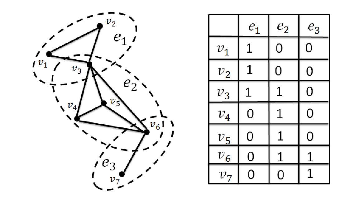
From the above definition, the main difference between a hypergraph and a pair-wise graph (For convenience, we call it simple graph in the following) lies in that a hyperedge can link more than two vertices. Thus, the hypergraph acts as a good model to represent local group information and complex relationship between samples. Taking Fig. 1 as an example, there are seven data points, and they are attributed to three local groups. One may construct a simple graph, in which two vertices are joined together by an edge if they are similar. However, simple graph cannot represent the group information well due to its pair-wise links. Different from a simple graph, a hypergraph can enclose a local group as one hyperedge according to the matrix shown in the right of Fig. 1. Thus, the constructed hypergraph is able to represent the local group information hidden in the data.
III Elastic Net Hypergraph
The hypergraph has been proposed as a natural way to encode higher order relationships in unsupervised and semi-supervised learning. By enclosing all the vertices with common attributes or close relationships within one hyperedge, we can effectively describe the high-order information of the data. Nevertheless, how to discover the related samples to form hyperedges and compute their weights is the key issue in the hypergraph construction. Most previous works have adopted the KNN method to generate the hyperedge, whereby each sample and its nearest neighbors form a hyperedge [25], [26]. The method is very simple, but it is not adaptive to local data distribution and some inherent information may be lost in the construction of hypergraphs.
In this section, we propose a process for constructing the so-called elastic net hypergraph (ENHG), in which each sample acts as a vertex and the hyperedge associated with each sample describes its robust elastic net driven reconstruction from the remaining samples. A robust matrix elastic net model is first designed for discovering the group structures and relationships hidden in the data. For each data point, we find the canonically related samples from the remaining samples to reconstruct it by the elastic net model. We then use the non-zero prominent elements of the representation to adaptively seek the most relevant neighbors to form a hyperedge, so that the data points in that hyperedge have strong dependencies. By regarding the elastic net representation of each data point as a feature, we compute the hyperedge weight by the sum of the mutual affinity between two data points calculated by the dot product between two features. The details are presented in the following sub-section.
III-A Robust Matrix Elastic Net for Group Representation
For a general data clustering or classification problem, the training sample set is assumed to be stacked as a matrix , whose columns are data points drawn from dimensional feature space. In practice, the data points may be contaminated by gross error ,
| (4) |
where and represent the clean data and the observed data respectively, is the error matrix. The -th sample is contaminated by error , which can present as noise, missed entries, outliers and corruption. Then the clean data can be represented by a linear combination of atoms from the dictionary ( is the atom number of ) as:
| (5) |
where is the coefficient matrix, and is the representation of upon the dictionary . The dictionary is often redundant and over-complete. Hence there can be many feasible solutions to problem (5). A popular method is to impose the common sparsity criteria, known as sparse linear representation. Intuitively, the sparsity of the coding coefficient vector can be measured by the norm to count the nonzero coefficients in the representation. It has been shown that under certain conditions, the norm optimization can provide us the sparse solution with similar nonzero supports as the norm optimization [28].
From the view of variable selection, the sparse linear representation problem can be cast as a problem of sparse covariate selection via a linear regression model by taking the dictionary matrix as an observation of the covariate and the query matrix as the response [14]. The norm constrained sparse linear representation can be regarded as a LASSO model, which seeks to predict an output by linearly combining a small subset of the features that describe the data. As a result of efficient optimization algorithms and the well-developed theory for generalization properties and variable selection consistency, the norm regularization has become a popular tool for variable selection and model estimation. However, the norm has its shortcomings in that each variable is estimated independently, regardless of its position in the input feature vector. If there is a group of variables among which the pair-wise correlations are very high, then LASSO tends to select only one variable from the group and does not care which one is selected. It lacks the ability to reveal the grouping information. It has been empirically observed that if there are high correlations between predictors, the prediction performance of LASSO is dominated by ridge regression. To overcome these limitations, the elastic net adds a quadratic part to the regularization, which can be regarded as a combination of LASSO and ridge regression. Here we take sample-specific corruption as an example, indicates the phenomenon that a fraction of the data points (i.e., columns of the data matrix ) is contaminated by a large error. By using the sample set itself as the dictionary, the matrix elastic net is modeled by
| (6) |
where the “entrywise” norm of the matrix is defined by , is the Frobenius norm of the matrix , denotes the mixed norm for dealing with sample-specific corruptions, computed as the sum of the norm of the columns of the matrix: , is the weight parameter of the quadratic part and is the regularization parameter to trade off the proportion and . An additional constraint is introduced, which is used to avoid the trivial solution of representing a point as a linear combination of itself. In other words, each datum is reconstructed by the linear combination of the remaining samples, which can be used to discover the group structures and relationships hidden in the data. The elastic net regularization encourages the grouping effect, favoring the selection of multiple correlated data points to represent the test sample.
Now we start out to solve the model (6). First, by replacing with , we can transform Eq. (6) into the following equivalent equation,
| (7) |
This objective function is to obtain the elastic net decomposition of all the samples, which can be indeed solved in a column-by-column fashion. Namely, it is equivalent to solve the elastic net decomposition of each sample respectively. Inspired by [10], we cope with the constraint by eliminating the sample from the sample matrix and the elastic net decomposition of sample can be formulated as,
| (8) |
where the dictionary matrix and the decomposition coefficient . It can be found that Eq. (8) is a typical elastic net model as in [15]. Thus, we directly adopt the LARS-EN algorithm [15],[13] to solve Eq. (8), which can compute the entire elastic net regularization paths with the computational effort of a single ordinal least squares fit. Since Eq. (8) is a convex problem, LARS-EN has been proved to converge to the global minimizer. After all the samples have been processed, the coefficient matrix can then be augmented as dimensional matrix by adding zero to the diagonal elements. Finally, we can obtain the coefficient matrix and the clean data from the given observation matrix , the gross error can be accordingly computed as . In terms of the reconstruction relationship of each vertex, we can define the hyperedge as the current vertex and its reconstruction, and predict the cluster or label information through the hypergraph defined on the obtained elastic net representation.
III-B Hyperedge construction
Given the data, each sample forms a vertex of the hypergraph , and can be represented by the other samples as in Eq. (6), where is its sparse coefficients, naturally characterizing the importance of the other samples for the reconstruction of . Such information is useful for recovering the clustering relationships among the samples. Although there are many zero components in , sample is mainly associated with only a few samples with prominent non-zero coefficients in its reconstruction. Thus, we design a quantitative rule to select the prominent samples and define the incidence matrix of an ENHR as:
| (9) |
where is a small threshold. For example, can be set as the mean values of . It can be seen that a vertex is assigned to based on whether the reconstruction coefficients is greater than the threshold . We take each sample as a centroid and form a hyperedge by the centroid and the selected most relevant samples in the elastic net reconstruction. The number of neighbors selected by Eq. (9) is adaptive to each datum, which is be propitious to capture the local grouping information of non-stationary data.
III-C Computation of hyperedge weights
The hyperedge weight also plays an important role in the hypergraph model. In [27], the non-zero coefficients are directly taken to measure the pair-wise similarity between two samples in the hyperedge. This is unreasonable, because the non-zero coefficients naturally represent the reconstruction relationship, but not the explicit degree of similarity. In this paper, we take each sparse representation vector as the sparse feature of , and we measure the similarity between two samples by the dot product of two sparse vectors as
| (10) |
The affinity matrix can be calculated as: , and the hyperedge weight is computed as follows:
| (11) |
Based on this definition, the compact hyperedge (local group) with higher inner group similarities is assigned a higher weight, and a weighted hypergraph is subsequently constructed. The ENHG model construction is summarized in Algorithm 1.
IV Learning with Elastic net Hypergraph
A well-designed graph is critical for those graph-oriented learning algorithms. In this section, we briefly introduce how to benefit from ENHG for clustering and classification tasks. Based on the proposed ENHG model, a hypergraph Laplacian matrix is constructed to find the spectrum signature and geometric structure of the data set for subsequent image analysis. Then, we formulate two learning tasks, i.e., spectral clustering and semi-supervised classification for image analysis formulated in terms of operations on our elastic net hypergraph. The principal idea is to perform spectral decomposition on the Laplacian matrix of the hypergraph model to obtain its eigenvectors and the eigenvalues [18]. Our elastic net hypergraph Laplacian matrix is also computed as
| (12) |
where and are the diagonal matrix of the vertex degrees and the hyperedge degrees, respectively. Based on the elastic net hypergraph model and its Laplacian matrix, we can design different learning algorithms.
IV-A Hypergraph spectral clustering
Clustering, or partitioning similar items into dissimilar groups, is widely used in data analysis and is applied in various areas such as, statistics, computer science, biology and social sciences. Spectral clustering is a popular algorithm for this task and is a powerful technique for partitioning simple graphs. Following [18], we develop an ENHR-based spectral clustering method. The main steps of spectral clustering based on ENHG are as follows:
- 1.
Calculate the normalized hypergraph Laplacian matrix by Eq. (12).
- 2.
Calculate the eigenvectors of L corresponding to the first k eigenvalues (sorted ascendingly), denoting the eigenvectors by .
- 3.
Denote the -th row of by , clustering the points in with K-Means algorithm into clusters .
- 4.
Finally, assign to cluster if the th row of the matrix is assigned to cluster .
IV-B Hypergraph Semi-supervised classification
Now we consider semi-supervised learning on ENHG. Given an ENHG model , each vertex represents a data point, is the total number of samples/vertices. Partial samples are labeled as from a label set ; is the total number of categories and the remaining samples are unlabeled. The goal of hypergraph semi-supervised learning is to predict the labels of the unlabeled samples according to the geometric structure of the hypergraph [18], [29], [30]. Due to the strong similarity of the data in a hyperedge, we try to assign the same label to all the vertices contained in the same hyperedge, and it is then straightforward to derive a semi-supervised prediction from a clustering scheme. Define a non-negative matrix corresponding to a classification on the by labeling each vertex with a label . We can understand as a vectorial classification function , which assigns a label vector to a vertex .
The hypergraph semi-supervised learning model can be formulated as the following regularization problem,
| (13) |
where is a regularizer on the hypergraph, is an empirical loss, and is the regularization parameter. The regularizer on the hypergraph is defined by
| (14) |
where is the matrix trace, and is the normalized hypergraph Laplacian matrix. Eq. (14) measures how smoothly the classification function defined on these points (vertices) changes with respect to their neighborhoods within the hyperedge. For the empirical loss, we define an matrix with if is labeled as and otherwise. Note that is consistent with the initial labels assigned according to the decision rule. To force the assigned labels to approach the initial labeling , the empirical loss can be defined as follows:
| (15) |
Differentiating the regularization framework with respect to , we can obtain a linear system for achieving the classification matrix . With the least square loss function, as shown in [18], the classification matrix can be directly given by with iterations, where , is a parameter in (0, 1). The predicted label for each point is determined using:
| (16) |
IV-C Discussions


Based on the above description, we can find that the computation of the Laplacian matrix plays a key role in the two learning algorithms. Here, we discuss the construction of our elastic net hypergraph Laplacian matrix, specifically the hyperedge construction, through a series of experiments. The quantitative results of the two learning algorithms upon the face and handwritten digits databases and comparison with other algorithms will be presented in Section V.
The authors of [15] have argued that the elastic net promotes the group selection of canonically related samples. Qualitatively speaking, a regression method exhibits the grouping effect if the regression coefficients of a group of highly correlated variables tend to be equal (up to a change of sign if negatively correlated). Theorem 1 of [15] pointed out the quantitative relationship between the consistency of sample ’s and ’s coefficient paths and their correlation . To empirically inspect the group selection effect of our elastic net model, we perform a number of evaluation experiments on the Extended Yale Face Database B [31] and examine the consistency of the solution path. We select the first four individuals as the sample set . Each individual has 64 near frontal images under different illuminations. We take each sample as a vertex, so the hypergraph size is equal to the number of training samples, and is the sample matrix. The evaluation experiment on the fifth face image of the first individual is presented for illustration. The response image (the fifth image) and partial predictor images (6th to 15th) are shown in Fig. 2.
Fig. 3 compares the solution path of the fifth face image of the first individual (response) in our elastic net model and the LASSO model. The coefficient paths of the sixth to fifteenth samples (predictor) in the LASSO and the elastic net model are displayed. We adopt as the horizontal axis. The vertical axis represents the coefficients value of each predictor. The LASSO paths are unstable and unsmooth. In contrast, the elastic net has much smoother solution paths, and the coefficient paths of highly related samples tend to coincide with each other, which clearly shows the group selection effect. Fig. 4 presents the reconstruction coefficients of the fifth face image of the first individual using the LASSO model and our elastic net model respectively. The parameter is set as 0.02 for our model and as 2.6 for LASSO, such that the two models find roughly the same number of non-zero coefficients. A number of highly correlated samples surrounding the prominent samples are selected in the elastic net, which also demonstrates the group selection effect. However, the prominent samples spread independently in the LASSO model.
Fig. 5 depicts the coefficients matrix of KNN, LASSO and our elastic net on the first four individuals of the Extended Yale B face database. The KNN method employs the Gaussian kernel function to find 45 neighbors of each sample. As with the KNN method, LASSO and our elastic net only keeps the first 45 large coefficients of each sample. The face samples are arranged sequentially according to their category. Thus, the ideal coefficient matrix should have the block diagonal structure. However, the KNN method has many large coefficients deviating from the main diagonal. LASSO and our Elastic Net has a distinct diagonal structure nevertheless. The prominent coefficient of our elastic net method gather more closely along the main diagonal than the LASSO method. It demonstrates that our method is more capable of finding correct neighbors than the LASSO method.


To evaluate the robustness of the hyperedge construction in our elastic net hypergraph, we select the first ten individuals as the sample set. Each individual has 64 samples, thus there are 640 samples in total and 640 vertices in the constructed hypergraph accordingly. Among the sample set, a sample from the first individual is used as the response for illustration and the remaining 639 samples are utilized as the dictionary to represent this response sample image. Fig. 6 shows the results. The horizontal axis indicates the index number of the samples in the dictionary and the index range is 1 to 639. The vertical axis indicates the distribution of the reconstruction coefficients for the remaining samples in the elastic net, and the response samples contaminated by the increasing degree of corruption (sparse noise and data missing) are shown in the right column. Those samples for which the coefficients are beyond the threshold indicated by the red dash line are enclosed by the hyperedge. By this selection strategy, the number of neighbors, i.e. the size of the hyperedge in ENHG, is adaptive to distinctive neighborhood structure of each datum, which is valuable for applications with non-homogeneous data distributions. Although the sparse error increases in the response sample, the distribution of the prominent samples in the elastic net does not show significant changes and the indices of the prominent samples beyond the threshold remain. The main reason for this stability is that the elastic net model can sperate the error from the corrupted sample. Fig. 7 shows the extracted components of some face images. We can see that our model can effectively remove the shadow. Compared with the hypergraphs constructed by the KNN and -neighborhood methods, the proposed elastic net hypergraph (ENHG) has two inherent advantages. First, ENHG is robust owing to the elastic net reconstruction from the remaining samples and the explicit consideration of data corruption. Second, the size of each hyperedge is datum-adaptive and automatically determined instead of uniformly global setting in the KNN and -neighborhood methods.
V Experiment Results and Analysis
We conduct the experiments on three public databases: the Extended Yale face database B [31], the PIE face database, and the USPS handwritten digit database [32], which are widely used to evaluate clustering and classification algorithms.
- •
Extended Yale Face Database B: This database has 38 individuals, and each subject has approximately 64 near frontal images under different illuminations. Following to [31], we crop the images by fixing the eyes and resize them to the size of , and we select the first 10, 15, 20, 30 and full subject set for the respective experiments.
- •
PIE Face Database: This database contains 41368 images of 68 subjects with different poses, illumination and expressions. Similar to [33], we select the first 15 and 25 subjects and only use the images of five near frontal poses (C05, C07, C09, C27, C29) under different illuminations and expressions. Each image is cropped and resized to the size of .
- •
USPS Handwritten Digital Database: This database contains ten classes (0-9 digit characters) and 9298 handwritten digit images in total. 200 images are randomly selected from each category for experiments. All of these images are normalized to the size of pixels.


Fig. 8 shows the sample images from the above three databases. As in [34], we normalize the samples so that they have a unit norm. To further evaluate the performance of the proposed methods, we compare them to seven state-of-the-art graph-based algorithms including:
- •
G-graph: We adopt Euclidean distance as our similarity measure, and use a Gaussian kernel to compute a weight for each edge of the graph.
- •
LE-graph: Following the example of [7], we construct the LE-graph, which used in Laplacian EigenMaps algorithm.
- •
- •
KNN-hypergraph (KNN-HG): Following [25], [26], we first use the Euclidean distance as the similarity measure. Each sample chooses eight nearest neighbors to construct the hyperedge, then transforms the hypergraph into an induced graph whose edge weights are normalized by the degree of the hyperedge.
- •
Semantic correlation hypergraph (SCHG): Following [27], we construct a semantic correlation hypergraph and each hyperedge is constructed by the index of the top five reconstruction coefficients from the sparse representation, hyperedge weights are then derived by these coefficients.
- •
Sparse Subspace Clustering (SSC): By representing each sample as the sparse combination of all the other data points, spectral clustering is used to obtain the clustering of the data [3].
- •
Low Rank Representation (LRR): This algorithm [4] sought the lowest-rank representation among all the candidates, which is used to define the weighted pairwise graph for spectral clustering.
For the sake of evaluating the effect of ENHG, we also implement a -Hypergraph algorithm, in which the elastic net is replaced by the original norm constrained sparse representation in the hyperedge construction.
The parameter and of the ENHG model are estimated by cross-validation, and we find that =0.01 and =0.18 is a proper parameter setting. The parameters of all the other algorithms are also tuned for optimal results. All the algorithms are implemented in Matlab R2011b running on Windows7, with an Intel (R)-Core(TM) i7-2600 3.40GHz processor and 16GB memory. The experiments are run 10 times and their average results are reported.
V-A Spectral clustering experiments
We carry out the spectral clustering experiments on two face databases and the USPS digital database. Two popular metrics, accuracy (AC) and normalized mutual information (NMI) [10], are used for quantitative performance evaluation.
The experimental results are listed in Tables II-IV respectively. From the results, it can be seen that the ENHG-based spectral clustering algorithm achieves better performance than the other five algorithms. The superiority of ENGH is mainly credited to the utilization of the elastic net to find the overall contextual information for constructing the hyperedge and computing weight. The Hypergraph-based algorithms mostly obtain better accuracy than the corresponding graph-based algorithms, which shows that the high-order local group information among the data is very useful for clustering. Meanwhile, ENGH can still obtain good clustering results on the Extended Yale B database with large shadow, which demonstrates its robustness to noise and error in the samples.
| YaleB | Metric | G-graph | LE-graph | -graph | SSC | LRR | KNN-HG | SCHG | -Hypergraph | ENHG |
| Cluster# | ||||||||||
| K=10 | AC | 0.172 | 0.420 | 0.758 | 0.821 | 0.822 | 0.507 | 0.775 | 0.873 | 0.928 |
| NMI | 0.091 | 0.453 | 0.738 | 0.811 | 0.814 | 0.495 | 0.702 | 0.846 | 0.922 | |
| K=15 | AC | 0.136 | 0.464 | 0.762 | 0.801 | 0.816 | 0.494 | 0.791 | 0.896 | 0.921 |
| NMI | 0.080 | 0.494 | 0.759 | 0.767 | 0.802 | 0.464 | 0.749 | 0.866 | 0.914 | |
| K=20 | AC | 0.113 | 0.478 | 0.793 | 0.797 | 0.801 | 0.534 | 0.782 | 0.884 | 0.918 |
| NMI | 0.080 | 0.492 | 0.786 | 0.781 | 0.792 | 0.485 | 0.742 | 0.866 | 0.912 | |
| K=30 | AC | 0.08 | 0.459 | 0.821 | 0.819 | 0.807 | 0.512 | 0.773 | 0.876 | 0.911 |
| NMI | 0.090 | 0.507 | 0.803 | 0.814 | 0.806 | 0.484 | 0.737 | 0.856 | 0.933 | |
| K=38 | AC | 0.08 | 0.443 | 0.785 | 0.794 | 0.785 | 0.486 | 0.764 | 0.826 | 0.881 |
| NMI | 0.110 | 0.497 | 0.776 | 0.787 | 0.781 | 0.473 | 0.723 | 0.804 | 0.915 |
| PIE | Metric | G-graph | LE-graph | -graph | SSC | LRR | KNN-HG | SCHG | -Hypergraph | ENHG |
| Cluster# | ||||||||||
| K=15 | AC | 0.144 | 0.158 | 0.786 | 0.798 | 0.802 | 0.554 | 0.792 | 0.801 | 0.821 |
| NMI | 0.090 | 0.114 | 0.762 | 0.803 | 0.813 | 0.503 | 0.769 | 0.775 | 0.839 | |
| K=25 | AC | 0.131 | 0.149 | 0.771 | 0.782 | 0.794 | 0.554 | 0.781 | 0.788 | 0.813 |
| NMI | 0.087 | 0.106 | 0.753 | 0.766 | 0.760 | 0.503 | 0.763 | 0.757 | 0.828 |
| USPS | Metric | G-graph | LE-graph | -graph | SSC | LRR | KNN-HG | SCHG | -Hypergraph | ENHG |
| Cluster # | ||||||||||
| K=4 | AC | 0.516 | 0.711 | 0.980 | 0.989 | 0.992 | 0.911 | 0.986 | 0.990 | 0.996 |
| NMI | 0.482 | 0.682 | 0.968 | 0.969 | 0.971 | 0.803 | 0.970 | 0.972 | 0.984 | |
| K=6 | AC | 0.424 | 0.69 | 0.928 | 0.936 | 0.957 | 0.871 | 0.925 | 0.945 | 0.980 |
| NMI | 0.351 | 0.542 | 0.917 | 0.928 | 0.937 | 0.762 | 0.916 | 0.927 | 0.942 | |
| K=8 | AC | 0.412 | 0.602 | 0.898 | 0.908 | 0.910 | 0.779 | 0.907 | 0.910 | 0.955 |
| NMI | 0.252 | 0.503 | 0.905 | 0.894 | 0.903 | 0.641 | 0.882 | 0.910 | 0.911 | |
| K=10 | AC | 0.338 | 0.582 | 0.856 | 0.881 | 0.889 | 0.765 | 0.801 | 0.886 | 0.932 |
| NMI | 0.213 | 0.489 | 0.872 | 0.866 | 0.871 | 0.636 | 0.822 | 0.870 | 0.874 |
| Dataset | G-graph | LE-graph | -graph | KNN-HG | SCHG | -Hypergraph | ENHG |
|---|---|---|---|---|---|---|---|
| Extended Yale B (10%) | 66.49 | 70.79 | 76.34 | 71.80 | 77.68 | 82.15 | 90.71 |
| Extended Yale B (20%) | 65.34 | 69.97 | 80.46 | 75.54 | 81.80 | 83.48 | 92.36 |
| Extended Yale B (30%) | 33.72 | 71.85 | 81.90 | 77.67 | 82.84 | 85.36 | 93.94 |
| Extended Yale B (40%) | 66.28 | 71.34 | 83.61 | 80.59 | 83.55 | 86.90 | 94.34 |
| Extended Yale B (50%) | 66.90 | 71.60 | 84.75 | 80.80 | 84.48 | 87.08 | 95.07 |
| Extended Yale B (60%) | 67.52 | 71.48 | 88.48 | 81.79 | 89.46 | 90.42 | 95.28 |
| PIE (10%) | 65.72 | 67.75 | 78.29 | 68.74 | 79.35 | 80.24 | 88.32 |
| PIE (20%) | 66.94 | 69.58 | 82.82 | 70.18 | 84.74 | 84.55 | 94.93 |
| PIE (30%) | 69.89 | 73.48 | 87.94 | 74.39 | 88.78 | 89.29 | 96.47 |
| PIE (40%) | 71.54 | 76.38 | 90.99 | 76.14 | 90.33 | 91.75 | 97.32 |
| PIE (50%) | 73.04 | 78.35 | 93.39 | 78.76 | 92.66 | 93.71 | 97.65 |
| PIE (60%) | 74.91 | 80.44 | 95.00 | 79.95 | 94.12 | 94.87 | 98.44 |
| USPS (10%) | 96.87 | 96.79 | 88.33 | 96.51 | 97.08 | 97.20 | 97.36 |
| USPS (20%) | 97.78 | 97.90 | 91.11 | 98.17 | 98.12 | 98.29 | 98.27 |
| USPS (30%) | 98.45 | 98.47 | 93.08 | 98.78 | 98.87 | 98.85 | 98.90 |
| USPS (40%) | 98.80 | 98.82 | 95.96 | 99.08 | 99.08 | 99.10 | 99.08 |
| USPS (50%) | 99.18 | 99.14 | 97.31 | 99.39 | 99.41 | 99.39 | 99.40 |
| USPS (60%) | 99.35 | 99.28 | 98.86 | 99.51 | 99.50 | 99.52 | 99.54 |
V-B Semi-supervised classification experiments
We also use the above three databases to evaluate the performance of semi-supervised classification. For the Extended Yale B and PIE databases, we randomly select 50 images from each subject in each run. The Extended Yale B and the first 15 subjects of PIE are used for evaluation. Of these images, the percentage of the labeled images ranges from 10% to 60%. For the USPS database, the ten digits are used and 200 images are randomly selected from each category for the experiments. These images are randomly labeled with different ratio as in the face databases. The accuracy rate is used to measure the classification performance as in [10], [34], [35]. The experimental results are reported in Table V. We can see that the ENHG method almost always achieves the best classification accuracy compared to the other five methods. The Hypergraph-based methods essentially outperform the pair-wise graph based methods. -Hypergraph has an evident advantage over -Graph, which shows that the high-order modeling ability of the hypergraph is very useful for semi-supervised learning. ENHG outperforming of -Hypergraph indicates that the elastic net can represent group structure hidden in the data more effectively. ENHG is also better than SCHG, because the hyperedges in ENHG are adaptive to local data distribution and the weight computation is more reasonable.
V-C Parameters analysis
In our proposed method, there are two regularization parameters, i.e., and . balances the importance between the norm and the norm. is the regularization parameter to trade off the proportion between the component and the component. We design two experiments to evaluate the influence of the two parameters on the results. We first analyze the influence of . The first ten individuals of the Extended Yale Face Database B are used as the sample set. We fix as 0.08, 0.18 and 1.8, and then sample ten points for in the range [0, 1000] for each value of . The AC and NMI scores of spectral clustering as a function of for several values of are plotted in Fig. 9. The semi-supervised classification results with 30% labeled samples are presented in Fig. 10. With regard to three values of , the curves of AC and NMI scores share similar changing trends and the maximum values of different curves are close to each other. When is set to 0, our model is identical to the LASSO. With ranging in [0.001, 1], the score index climbs slowly and stays for a while, which demonstrates the effectiveness of the elastic net regularization. With increasing to 1000, our model tends to be closer to ridge regression and thus the score drops rapidly.
Furthermore, we turn to the parameter. The first ten individuals of the Extended Yale Face Database B are also employed as the sample set. Each sample is normalized to have the unit length. In order to test the influence of the parameter and validate the robustness of our model to noise, 25% percentages of samples are randomly chosen to be corrupted by Gaussian noise, i.e., for a sample vector chosen to be corrupted, its observed vector is computed by adding Gaussian noise with zero mean and variance 0.1. Fixing as 0.01, 1 and 10, we run our model with different for each value of . Fig. 11 plots the spectral clustering results with ENHG. When is small, the component cannot reconstruct the sample matrix , and is not capable of representing the relationship between samples. Thus, the AC and NMI score are low. As roughly increases to 0.2, can represent the reconstruction relationship effectively, and noise component may be well separated from . The AC and NMI scores reach the top at this time. With continually increasing to 10, the noise component cannot be removed well and the AC and NMI scores decrease slowly. Fig. 12 presents the semi-supervised classification results, which are similar to the spectral clustering results. However, the changing range of semi-supervised classification is smaller than spectral clustering. The value of controls the proportion of norm in the constraint. Although the curves of AC and NMI scores corresponding to each value of demonstrate a similar pattern of variability, the maximum scores of each curve are certainly different.


VI Conclusions
This paper proposed a novel elastic net hypergraph (ENHG) for two learning tasks, namely spectral clustering and semi-supervised classification, which has three important properties: adaptive hyperedge construction, reasonable hyperedge weight calculation, and robustness to data noise. The hypergraph structure and the hyperedge weights are simultaneously derived by solving a problem of robust elastic net representation of the whole data. Robust elastic net encourages a grouping effect, where strongly correlated samples tend to be simultaneously selected or rejected by the model. The ENHG represents the high order relationship between one datum and its prominent reconstruction samples by regarding them as a hyperedge. Extensive experiments show that ENHG is more effective and more suitable than other graphs for many popular graph-based machine learning tasks.
References
- [1] Jianbo Shi and Jitendra Malik, “Normalized cuts and image segmentation,” IEEE Transactions on Pattern Analysis and Machine Intelligence, vol. 22, no. 8, pp. 888–905, 2000.
- [2] Andrew Y Ng, Michael I Jordan, Yair Weiss, et al., “On spectral clustering: Analysis and an algorithm,” Advances in neural information processing systems, vol. 2, pp. 849–856, 2001.
- [3] Ehsan Elhamifar and Ren´ e Vidal, “Sparse subspace clustering: Algorithm, theory, and applications,” IEEE Transactions on Pattern Analysis and Machine Intelligence, vol. 35, no. 11, pp. 2765–2781, 2013.
- [4] Liu Guangcan, Lin Zhouchen, and et al., “Robust recovery of subspace structures by low-rank representation,” IEEE Transactions on Pattern Analysis and Machine Intelligence, vol. 35, no. 1, pp. 171–184, 2013.
- [5] Joshua B Tenenbaum, Vin De Silva, and John C Langford, “A global geometric framework for nonlinear dimensionality reduction,” Science, vol. 290, no. 5500, pp. 2319–2323, 2000.
- [6] Sam T Roweis and Lawrence K Saul, “Nonlinear dimensionality reduction by locally linear embedding,” Science, vol. 290, no. 5500, pp. 2323–2326, 2000.
- [7] Mikhail Belkin and Partha Niyogi, “Laplacian eigenmaps for dimensionality reduction and data representation,” Neural computation, vol. 15, no. 6, pp. 1373–1396, 2003.
- [8] Xiaojin Zhu, “Semi-supervised learning literature survey,” Computer Science, vol. 37, no. 1, pp. 63–67, 2008.
- [9] Xiaojin Zhu, Zoubin Ghahramani, John Lafferty, et al., “Semi-supervised learning using gaussian fields and harmonic functions,” in International Conference on Machine Learning, 2003, pp. 912–919.
- [10] Bin Cheng, Jianchao Yang, Shuicheng Yan, Yun Fu, and Thomas S Huang, “Learning with -graph for image analysis.,” IEEE Transactions on Image Processing, vol. 19, no. 4, pp. 858–866, 2010.
- [11] Ran He, Wei-Shi Zheng, Bao-Gang Hu, and Xiang-Wei Kong, “Nonnegative sparse coding for discriminative semi-supervised learning,” in IEEE Conference on Computer Vision and Pattern Recognition, 2011, pp. 2849–2856.
- [12] Jinhui Tang, Richang Hong, Shuicheng Yan, Tat-Seng Chua, Guo-Jun Qi, and Ramesh Jain, “Image annotation by knn-sparse graph-based label propagation over noisily tagged web images,” ACM Transactions on Intelligent Systems and Technology, vol. 2, no. 2, pp. 135–136, 2011.
- [13] Johnstone Iain Efron Bradley, Hastie Trevor and Tibshirani Robert, “Least angle regression,” Annals of Statistics, vol. 32, no. 2, pp. 407–499, 2004.
- [14] Yuan XiaoTong, Liu Xiaobai, and Yan Shuicheng, “Visual classification with multitask joint sparse representation,” IEEE Transactions on Image Processing, vol. 21, no. 10, pp. 4349–4360, 2012.
- [15] Hui Zou and Trevor Hastie, “Regularization and variable selection via the elastic net,” Journal of the Royal Statistical Society B, vol. 67, no. 2, pp. 301–320, 2005.
- [16] E. Elhamifar and R. Vidal, “Robust classification using structured sparse representation,” 2010, pp. 1873–1879.
- [17] László Lovász, “Minimax theorems for hypergraphs,” in Hypergraph seminar, 1974, pp. 111–126.
- [18] Dengyong Zhou, Jiayuan Huang, and Bernhard Schölkopf, “Learning with hypergraphs: Clustering, classification, and embedding,” Advances in Neural Information Processing Systems, vol. 19, pp. 1601–1608, 2006.
- [19] Sameer Agarwal, Kristin Branson, and Serge Belongie, “Higher order learning with graphs,” in International Conference on Machine Learning, 2006, pp. 17–24.
- [20] Sameer Agarwal, Jongwoo Lim, Lihi Zelnik-Manor, Pietro Perona, David Kriegman, and Serge Belongie, “Beyond pairwise clustering,” in IEEE Computer Society Conference on Computer Vision and Pattern Recognition,, 2005, vol. 2, pp. 838–845.
- [21] Ron Zass and Amnon Shashua, “Probabilistic graph and hypergraph matching,” in IEEE Conference on Computer Vision and Pattern Recognition, 2008, pp. 1–8.
- [22] Liang Sun, Shuiwang Ji, and Jieping Ye, “Hypergraph spectral learning for multi-label classification,” in Proceedings of the 14th ACM SIGKDD international conference on Knowledge discovery and data mining, 2008, pp. 668–676.
- [23] Yuchi Huang, Qingshan Liu, and Dimitris Metaxas, “Video object segmentation by hypergraph cut,” in IEEE Conference on Computer Vision and Pattern Recognition, 2009, pp. 1738–1745.
- [24] Ze Tian and Rui Kuang, “Integrative classification and analysis of multiple arraycgh datasets with probe alignment,” Bioinformatics, vol. 26, no. 18, pp. 2313–2320, 2010.
- [25] Yuchi Huang, Qingshan Liu, Shaoting Zhang, and Dimitris N Metaxas, “Image retrieval via probabilistic hypergraph ranking,” in IEEE Conference on Computer Vision and Pattern Recognition, 2010, pp. 3376–3383.
- [26] Yuchi Huang, Qingshan Liu, Fengjun Lv, Yihong Gong, and Dimitris N Metaxas, “Unsupervised image categorization by hypergraph partition,” IEEE Transactions on Pattern Analysis and Machine Intelligence, vol. 33, no. 6, pp. 1266–1273, 2011.
- [27] Chaoqun Hong and Jianke Zhu, “Hypergraph-based multi-example ranking with sparse representation for transductive learning image retrieval,” Neurocomputing, vol. 101, no. 4, pp. 94–103, 2013.
- [28] DL Donoho, “For most large underdetermined systems of linear equations the minimal l1-norm solution is also the sparsest solution,” Communications on pure and applied mathematics, vol. 56, no. 6, pp. 797–829, 2006.
- [29] Dengyong Zhou, Olivier Bousquet, Thomas Navin Lal, Jason Weston, and Bernhard Schölkopf, “Learning with local and global consistency,” Advances in neural information processing systems, vol. 17, no. 4, pp. 321–328, 2004.
- [30] Dengyong Zhou, Jiayuan Huang, and Bernhard Schölkopf, “Learning from labeled and unlabeled data on a directed graph,” in International Conference on Machine Learning, 2005, pp. 1036–1043.
- [31] Kuang-Chih Lee, Jeffrey Ho, and David J Kriegman, “Acquiring linear subspaces for face recognition under variable lighting,” IEEE Transactions on Pattern Analysis and Machine Intelligence, vol. 27, no. 5, pp. 684–698, 2005.
- [32] Jonathan J. Hull, “A database for handwritten text recognition research,” IEEE Transactions on Pattern Analysis and Machine Intelligence, vol. 16, no. 5, pp. 550–554, 1994.
- [33] D Cai X He, et al., “Graph regularized non-negative matrix factorization for data representation,” IEEE Transactions on Pattern Analysis and Machine Intelligence, vol. 33, no. 8, pp. 1548–1560, 2011.
- [34] John Wright, Yi Ma, Julien Mairal, Guillermo Sapiro, Thomas S Huang, and Shuicheng Yan, “Sparse representation for computer vision and pattern recognition,” Proceedings of the IEEE, vol. 98, no. 6, pp. 1031–1044, 2010.
- [35] Shuicheng Yan and Huan Wang, “Semi-supervised learning by sparse representation.,” in Proceedings of the SIAM International Conference on Data Mining, 2009, pp. 792–801.