1Introduction

CBMM Memo No. 045 August 24, 2026

Learning Functions: When Is Deep Better Than Shallow

Hrushikesh Mhaskar
Department of Mathematics, California Institute of Technology, Pasadena, CA 91125;
Institute of Mathematical Sciences, Claremont Graduate University, Claremont, CA 91711,
Qianli Liao and Tomaso Poggio
Center for Brains, Minds, and Machines, McGovern Institute for Brain Research
Massachusetts Institute of Technology, Cambridge, MA, 02139

Abstract: ¹¹ 1 This is an update of a previous version released on March 3rd 2016. While the universal approximation property holds both for hierarchical and shallow networks, we prove that deep (hierarchical) networks can approximate the class of compositional functions with the same accuracy as shallow networks but with exponentially lower number of training parameters as well as VC-dimension. This theorem settles an old conjecture by Bengio on the role of depth in networks. We then define a general class of scalable, shift-invariant algorithms to show a simple and natural set of requirements that justify deep convolutional networks.

This work was supported by the Center for Brains, Minds and Machines (CBMM), funded by NSF STC award CCF - 1231216.

1 Introduction

There are two main theory questions about Deep Neural Networks. The first question is about the power of the architecture – which classes of functions can it approximate well? The second question is about learning the unknown coefficients from the data: why is SGD so unreasonably efficient, at least in appearance? Are good minima easier to find in deep rather than in shallow networks? In this paper we describe a set of approximation theory results that include answers to why and when deep networks are better than shallow by using the idealized model of a deep network as a binary tree. In a separate paper, we show that the binary tree model with its associated results can indeed be extended formally to the very deep convolutional networks of the ResNet type which have only a few stages of pooling and subsampling.

This paper compares shallow (one-hidden layer) networks with deep networks (see for example Figure 1). Both types of networks use the same small set of operations – dot products, linear combinations, a fixed nonlinear function of one variable, possibly convolution and pooling. The logic of the paper is as follows.

•

Both shallow (a) and deep (b) networks are universal, that is they can approximate arbitrarily well any continuous function of $d$ variables on a compact domain.
•

We show that the approximation of functions with a compositional structure – such as $f(x_{1},\cdots,x_{d})=h_{1}(h_{2}\cdots(h_{j}(h_{i1}(x_{1},x_{2}),h_{i2}(x_{3},x_{4})),\cdots))$ – can be achieved with the same degree of accuracy by deep and shallow networks but that the number of parameters, the VC-dimension and the fat-shattering dimension are much smaller for the deep networks than for the shallow network with equivalent approximation accuracy. It is intuitive that a hierarchical network matching the structure of a compositional function should be “better” at approximating it than a generic shallow network but universality of shallow networks makes the statement less than obvious. Our result makes clear that the intuition is indeed correct and provides quantitative bounds.
•

Why are compositional functions important? We argue that the basic properties of scalability and shift invariance in many natural signals such as images and text require compositional algorithms that can be well approximated by Deep Convolutional Networks. Of course, there are many situations that do not require shift invariant, scalable algorithms. For the many functions that are not compositional we do not expect any advantage of deep convolutional networks.

2 Previous work

The success of Deep Learning in the present landscape of machine learning poses again an old theory question: why are multi-layer networks better than one-hidden-layer networks? Under which conditions? The question is relevant in several related fields from machine learning to function approximation and has appeared many times before.

Most Deep Learning references these days start with Hinton’s backpropagation and with Lecun’s convolutional networks (see for a nice review [LeCun et al., 2015]). Of course, multilayer convolutional networks have been around at least as far back as the optical processing era of the 70s. The Neocognitron ([Fukushima, 1980]) was a convolutional neural network that was trained to recognize characters. The HMAX model of visual cortex ([Riesenhuber and Poggio, 1999a]) was described as a series of AND and OR layers to represent hierarchies of disjunctions of conjunctions. There are several recent papers addressing the question of why hierarchies. Sum-Product networks, which are equivalent to polynomial networks (see [B. Moore and Poggio, 1998, Livni et al., 2013]), are a simple case of a hierarchy that can be analyzed ([Delalleau and Bengio, 2011]). [Montufar et al., 2014] provided an estimation of the number of linear regions that a network with ReLU nonlinearities can synthesize in principle but leaves open the question of whether they can be used for learning. Examples of functions that cannot be represented efficiently by shallow networks have been given very recently by [Telgarsky, 2015]. Most relevant to this paper is the work on hierarchical quadratic networks ([Livni et al., 2013]), together with function approximation results ([Pinkus, 1999, Mhaskar, 1993]).

3 Compositional functions

We assume that the shallow networks do not have any structural information on the function to be learned (here its compositional structure), because they cannot represent it directly. Deep networks with standard architectures on the other hand do represent compositionality and can be adapted to the details of such prior information. Thus, it is natural to conjecture that hierarchical compositions of functions such as

	$\displaystyle f(x_{1},\cdots,x_{8})=h_{3}(h_{21}(h_{11}(x_{1},x_{2}),h_{12}(x_{3},x_{4})),$				(1)
			$\displaystyle\qquad h_{22}(h_{13}(x_{5},x_{6}),h_{14}(x_{7},x_{8})))$		(1)

are approximated more efficiently by deep than by shallow networks.

In addition, both shallow and deep representations may or may not reflect invariance to group transformations of the inputs of the function ( [Soatto, 2011, Anselmi et al., 2015]). Invariance is expected to decrease the complexity of the network, for instance its VC-dimension. Since we are interested in the comparison of shallow vs deep architectures, here we consider the generic case of networks (and functions) for which invariance is not assumed.

We approximate functions of $d$ variables of the form of Equation (1) with networks in which the activation nonlinearity is a smoothened version of the so called ReLU, originally called ramp by Breiman and given by $\sigma(x)=x_{+}=max(0,x)$ . The architecture of the deep networks reflects Equation (1) with each node $h_{i}$ being a ridge function.

Refer to caption — Figure 1: a) A shallow universal network in 8 variables and $N$ units which can approximate a generic function $f(x_{1},\cdots,x_{8})$ . b) A binary tree hierarchical network in 8 variables, which approximates well functions of the form $f(x_{1},\cdots,x_{8})=h_{3}(h_{21}(h_{11}(x_{1},x_{2}),h_{12}(x_{3},x_{4})),\allowbreak h_{22}(h_{13}(x_{5},x_{6}),h_{14}(x_{7},x_{8})))$ . Each of the nodes in b) consists of $n$ ReLU units and computes the ridge function ([Pinkus, 1999]) $\sum_{i=1}^{n}a_{i}(\left\langle{\mathbf{v}_{i}},{\mathbf{x}}\right\rangle+t_{i})_{+}$ , with $\mathbf{v}_{i},\mathbf{x}\in\R^{2}$ , $a_{i},t_{i}\in\R$ . Each term, that is each unit in the node, corresponds to a “channel”. Similar to the shallow network a hierarchical network as in b) can approximate any continuous function; the text proves how it approximates a compositional functions better than a shallow network. No invariance is assumed here.

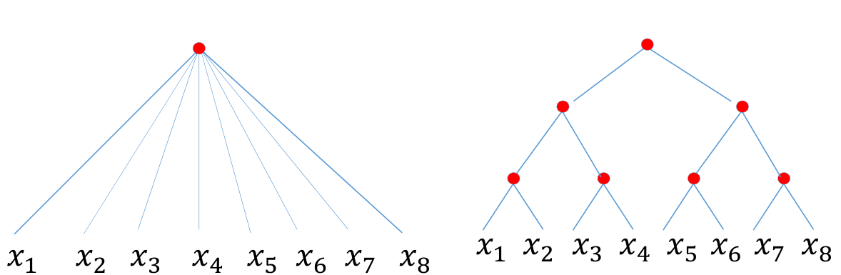
It is important to emphasize here that the properties of state-of-art Deep Learning Neural Networks (DLNNs) of the ResNet type ([He et al., 2015]), with their small kernel size and many layers, are well represented by our results on binary tree architectures, as we show formally elsewhere. Visual cortex has a similar compositional architecture with receptive fields becoming larger and larger in higher and higher visual areas, with each area corresponding to a recurrent layer in a deep neural network ([Liao and Poggio, 2016]).

4 Main results

In this section, we describe the approximation properties of the shallow and deep networks in two cases: deep networks with ReLU nonlinearities and deep Gaussian networks. The general paradigm is as follows. We are interested in determining how complex the network ought to be to theoretically guarantee that the network would approximate an unknown target function $f$ up to a given accuracy $\epsilon>0$ . To measure the accuracy, we need a norm $\|\cdot\|$ on some normed linear space $\mathbb{X}$ . The complexity of the network is indicated by a subscript to the general class of networks with this complexity; let $V_{n}$ the be set of all networks of a given kind with the complexity given by $n$ (e.g., all shallow networks with $n$ units in the hidden layer). It is assumed that the class of networks with a higher complexity include those with a lower complexity; i.e., $V_{n}\subseteq V_{n+1}$ . The degree of approximation is defined by

\mathsf{dist}(f,V_{n})=\inf_{P\in V_{n}}\|f-P\|.

(2)

For example, if $\mathsf{dist}(f,V_{n})=\mathcal{O}(n^{-\gamma})$ for some $\gamma>0$ , then one needs a network with complexity $\mathcal{O}(\epsilon^{-\gamma})$ to guarantee an approximation up to accuracy $\epsilon$ . It is therefore customary and easier to give estimates on $d(f,V_{n})$ in terms of $n$ rather than in terms of $\epsilon$ , inverse to $d(f,V_{n})$ . Since $f$ is unknown, in order to obtain theoretically proved upper bounds, we need to make some assumptions on the class of functions from which the unknown target function is chosen. This a priori information is codified by the statement that $f\in W$ for some subspace $W\subseteq\mathbb{X}$ . This subspace is usually referred to as the smoothness class. In general, a deep network architecture (in this paper, we restrict ourselves to the binary tree structure as in (1)) has an advantage over the shallow networks when the target function itself has the same hierarchical, compositional structure, e.g., (1).

4.1 Deep and shallow neural networks

We start with a review of previous results ([Mhaskar, 1996]). Let $I^{d}=[-1,1]^{d}$ , $\mathbb{X}=C(I^{d})$ be the space of all continuous functions on $I^{d}$ , with $\|f\|=\max_{\mathbf{x}\in I^{d}}|f(\mathbf{x})|$ . Let $\mathcal{S}_{n}$ denote the class of all shallow networks with $n$ units of the form

\mathbf{x}\mapsto\sum_{k=1}^{n}a_{k}\sigma(\mathbf{w}_{k}\cdot\mathbf{x}+b_{k}),

where $\mathbf{w}_{k}\in\R^{d}$ , $b_{k},a_{k}\in\R$ . The number of trainable parameters here is $(d+2)n\sim n$ . Let $r\geq 1$ be an integer, and $W_{r,d}^{\mbox{NN}}$ be the set of all functions with continuous partial derivatives of orders up to $r$ such that $\|f\|+\sum_{1\leq|\mathbf{k}|_{1}\leq r}\|D^{\mathbf{k}}f\|\leq 1$ , where $D^{\mathbf{k}}$ denotes the partial derivative indicated by the multi–integer $\mathbf{k}\geq 1$ , and $|\mathbf{k}|_{1}$ is the sum of the components of $\mathbf{k}$ .

For the hierarchical binary tree network, the analogous spaces are defined by considering the compact set $W_{H,r,2}^{\mbox{NN}}$ to be the class of all functions $f$ which have the same structure (e.g., (1)), where each of the constituent functions $h$ is in $W_{r,2}^{\mbox{NN}}$ (applied with only $2$ variables). We define the corresponding class of deep networks $\mathcal{D}_{n}$ to be set of all functions with the same structure, where each of the constituent functions is in $\mathcal{S}_{n}$ . We note that in the case when $d$ is an integer power of $2$ , the number of parameters involved in an element of $\mathcal{D}_{n}$ – that is, weights and biases, in a node of the binary tree is $(d-1)(d+2)n$ .

The following theorem estimates the degree of approximation for shallow and deep networks. We remark that the assumptions on $\sigma$ in the theorem below are not satisfied by the ReLU function $x\mapsto x_{+}$ , but they are satisfied by smoothing the function in an arbitrarily small interval around the origin.

Theorem 1.

Let $\sigma:\R\to\R$ be infinitely differentiable, and not a polynomial on any subinterval of $\R$ .
(a) For $f\in W_{r,d}^{\mbox{NN}}$

\mathsf{dist}(f,\mathcal{S}_{n})=\mathcal{O}(n^{-r/d}).

(3)

(b) For $f\in W_{H,r,d}^{\mbox{NN}}$

\mathsf{dist}(f,\mathcal{D}_{n})=\mathcal{O}(n^{-r/2}).

(4)

Proof. Theorem 1(a) was proved by [Mhaskar, 1996]. To prove Theorem 1(b), we observe that each of the constituent functions being in $W_{r,2}^{\mbox{NN}}$ , (3) applied with $d=2$ implies that each of these functions can be approximated from $\mathcal{S}_{n}$ up to accuracy $n^{-r/2}$ . Our assumption that $f\in W_{H,r,2}^{\mbox{NN}}$ implies that each of these constituent functions is Lipschitz continuous. Hence, it is easy to deduce that, for example, if $P$ , $P_{1}$ , $P_{2}$ are approximations to the constituent functions $h$ , $h_{1}$ , $h_{2}$ , respectively within an accuracy of $\epsilon$ , then

\|h(h_{1},h_{2})-P(P_{1},P_{2})\|\leq c\epsilon,

for some constant $c>0$ independent of the functions involved. This leads to (4). $\square$

The constants involved in $\mathcal{O}$ in (3) will depend upon the norms of the derivatives of $f$ as well as $\sigma$ . Thus, when the only a priori assumption on the target function is about the number of derivatives, then to guarantee an accuracy of $\epsilon$ , we need a shallow network with $\mathcal{O}(\epsilon^{-d/r})$ trainable parameters. If we assume a hierarchical structure on the target function as in Theorem 1, then the corresponding deep network yields a guaranteed accuracy of $\epsilon$ only with $\mathcal{O}(\epsilon^{-2/r})$ trainable parameters.

Is this the best? To investigate this question, let $M_{n}:W_{r,d}^{\mbox{NN}}\to\mathbb{R}^{n}$ be a continuous mapping (parameter selection), and $A_{n}:\mathbb{R}^{n}\to C(I^{d})$ be any mapping (recovery algorithm). Then an approximation to $f$ is given by $A_{n}(M_{n}(f))$ , where the continuity of $M_{n}$ means that the selection of parameters is robust with respect to perturbations in $f$ . The nonlinear $n$ –width of the compact set $W_{r,d}^{\mbox{NN}}$ is defined by (cf. [DeVore et al., 1989])

d_{n}(W_{r,d}^{\mbox{NN}})=\inf_{M_{n},A_{n}}\sup_{f\in W_{r,d}^{\mbox{NN}}}\|f-A_{n}(M_{n}(f))\|,

(5)

and the curse for $W_{r,d}^{\mbox{NN}}$ by

\mathsf{curse}(W_{r,d}^{\mbox{NN}},\epsilon)=\min\{n\geq 1:d_{n}(W_{r,d}^{\mbox{NN}})\leq\epsilon\}.

(6)

We note that the curse depends only on the compact set $W_{r,d}^{\mbox{NN}}$ , and represents the best that can be achieved by any continuous parameter selection and recovery processes. It is shown by [DeVore et al., 1989] that $\mathsf{curse}(W_{r,d}^{\mbox{NN}},\epsilon)\geq c\epsilon^{-d/r}$ for some constant $c>0$ depending only on $d$ and $r$ . So, the estimate implied by (3) is the best possible among all reasonable methods of approximating arbitrary functions in $W_{r,d}^{\mbox{NN}}$ , although by itself, the estimate (3) is blind to the process by which the approximation is accomplished; in particular, this process is not required to be robust. Similar considerations apply to the estimate (4), and we will explain the details in Section 4.2 in a different context.

The lower bound on the $n$ –width implies only that there is some function in $W_{r,d}^{\mbox{NN}}$ for which the approximation cannot be better than that suggested by (3). This begs the question whether this function could be unreasonably pathological, and for most functions arising in practice, clever ideas can lead to a substantially better accuracy of approximation, its smoothness notwithstanding. At this time, we are not able to address this question in the context of neural networks as in Theorem 1, but we are able to do so if each unit evaluates a Gaussian network. Accordingly, we now turn to our new results in this direction. The proofs will be published separately.

4.2 Deep and shallow Gaussian networks

We wish to consider shallow networks where each channel evaluates a Gaussian non–linearity; i.e., Gaussian networks of the form

G(\mathbf{x})=\sum_{k=1}^{N}a_{k}\exp(-|\mathbf{x}-\mathbf{x}_{k}|^{2}),\qquad\mathbf{x}\in\mathbb{R}^{d}.

(7)

It is natural to consider the number of trainable parameters $(d+1)N$ as a measurement of the complexity of $G$ . However, it is known ([Mhaskar, 2004]) that an even more important quantity that determines the approximation power of Gaussian networks is the minimal separation among the centers. For any subset $\mathcal{C}$ of $\mathbb{R}^{d}$ , the minimal separation of $\mathcal{C}$ is defined by

\eta(\mathcal{C})=\inf_{\mathbf{x},\mathbf{y}\in\mathcal{C},\mathbf{x}\not=\mathbf{y}}|\mathbf{x}-\mathbf{y}|.

(8)

For $N,m>0$ , the symbol $\mathcal{N}_{N,m}(\mathbb{R}^{d})$ denotes the set of all Gaussian networks of the form (7), with $\eta(\{\mathbf{x}_{1},\cdots,\mathbf{x}_{N}\})\geq 1/m$ .

Since it is our goal to make a comparison between shallow and deep networks, we will consider also deep networks organized for simplicity as a binary tree $\mathcal{T}$ , where each unit computes a network in $\mathcal{N}_{N,m}(\mathbb{R}^{2})$ . The set of all such networks will be denoted by $\mathcal{T}\mathcal{N}_{N,m}(\mathbb{R}^{2})$ . In this context, it is not natural to constrain the output of the hidden units to be in $[-1,1]$ . Therefore, we need to consider approximation on the entire Euclidean space in question. Accordingly, let $\mathbb{X}_{d}$ be the space $C_{0}(\mathbb{R}^{d})$ of continuous functions on $\mathbb{R}^{d}$ vanishing at infinity, equipped with the norm $\|f\|_{d}=\max_{\mathbf{x}\in\mathbb{R}^{d}}|f(\mathbf{x})|$ . For the class $W$ , we then need to put conditions not just on the number of derivatives but also on the rate at which these derivatives tend to $0$ at infinity. Generalizing an idea from [Freud, 1972, Mhaskar, 2003], we first define the space $W_{r,d}$ for integer $r\geq 1$ as the set of all functions $f$ which have $r$ continuous derivatives in $C_{0}(\mathbb{R}^{d})$ , satisfying

\|f\|_{r,d}=\|f\|_{d}+\sum_{1\leq|\mathbf{k}|_{1}\leq r}\|\exp(-|\cdot|^{2})D^{\mathbf{k}}(\exp(|\cdot|^{2})f\|_{d}<\infty.

Since one of our goals is to show that our results on the upper bounds for the accuracy of approximation are the best possible for individual functions, the class $W_{r,d}$ needs to be refined somewhat. Toward that goal, we define next a regularization expression, known in approximation theory parlance as a $K$ –functional, by

K_{r,d}(f,\delta)=\inf_{g\in W_{r,d}}\{\|f-g\|_{d}+\delta^{r}(\|g\|_{d}+\|g\|_{r,d})\}.

We note that the infimum above is over all $g$ in the class $W_{r,d}$ rather than just the class of all networks. The class $\mathcal{W}_{\gamma,d}$ of functions which we are interested in is then defined for $\gamma>0$ as the set of all $f\in C_{0}(\mathbb{R}^{d})$ for which

\|f\|_{\gamma,d}=\|f\|+\sup_{\delta\in(0,1]}\frac{K_{r,d}(f,\delta)}{\delta^{\gamma}}<\infty,

for some integer $r\geq\gamma$ . It turns out that different choices of $r$ yield equivalent norms, without changing the class itself. The following theorem gives a bound on approximation of $f\in C_{0}(\mathbb{R}^{d})$ from $\mathcal{N}_{N,m}$ . Here and in the sequel, we find it convenient to adopt the following convention. By $A\lesssim B$ we mean $A\leq cB$ where $c>0$ is a constant depending only on the fixed parameters of the discussion, such as $\gamma$ , $d$ . By $A\sim B$ , we mean $A\lesssim B$ and $B\lesssim A$ . The following theorems, as they apply to shallow networks, are technical improvements on those in [Mhaskar, 2004].

Theorem 2.

There exists a constant $c>0$ depending on $d$ alone with the following property. Let $\{\mathcal{C}_{m}\}$ be a sequence of finite subsets with $\mathcal{C}_{m}\subset[-cm,cm]^{d}$ , with

1/m\lesssim\max_{\mathbf{y}\in K}\min_{\mathbf{x}\in\mathcal{C}}|\mathbf{x}-\mathbf{y}|\lesssim\eta(\mathcal{C}_{m}),\qquad m=1,2,\cdots.

(9)

If $\gamma>0$ and $f\in\mathcal{W}_{\gamma,d}$ , then for integer $m\geq 1$ , there exists $G\in\mathcal{N}_{|\mathcal{C}_{m}|,m}$ with centers at points in $\mathcal{C}_{m}$ such that

\|f-G\|_{d}\lesssim\frac{1}{m^{\gamma}}\|f\|_{\gamma,d}.

(10)

Moreover, the coefficients of $G$ can be chosen as linear combinations of the data $\{f(\mathbf{x}):\mathbf{x}\in\mathcal{C}_{m}\}$ .

We note that the set of centers $\mathcal{C}_{m}$ can be chosen arbitrarily subject to the conditions stated in the theorem; there is no training necessary to determine these parameters. Therefore, there are only $\mathcal{O}(m^{2})$ coefficients to be found by training. This means that if we assume a priori that $f\in\mathcal{W}_{\gamma,d}$ , then the number of trainable parameters to theoretically guarantee an accuracy of $\epsilon>0$ is $\mathcal{O}(\epsilon^{-2d/\gamma})$ . We will comment on the optimality of this estimate later.

Next, we discuss approximation by deep networks in $\mathcal{T}\mathcal{N}_{N,m}(\mathbb{R}^{2})$ . We will show that the accuracy of the approximation increases dramatically if the target function $f$ is known to have the compositional hierarchical structure prescribed by $\mathcal{T}$ . It is not clear that this structure is unique. Therefore, for mathematical analysis, it is convenient to think of such a function $f$ as in fact a family of functions $\{f_{v}\}_{v\in V}$ , where $V$ is the set of non–leaf nodes in $\mathcal{T}$ , and $f_{v}$ is the constituent function evaluated at the vertex $v$ . The set of all such functions will be denoted by $\mathcal{T}C_{0}(\mathbb{R}^{2})$ . Likewise, a network $G\in\mathcal{T}\mathcal{N}_{N,m}(\mathbb{R}^{2})$ is thought of as the family of networks $\{G_{v}\}_{v\in V}$ , where each $G_{v}\in\mathcal{N}_{N,m}(\mathbb{R}^{2})$ . Accordingly, the norm in which the approximation error (respectively, the smoothness) is measured is defined by

\|f\|_{\mathcal{T}}=\sum_{v\in V}\|f_{v}\|_{2},\qquad\|f\|_{\mathcal{T}\mathcal{W}_{\gamma,2}}=\sum_{v\in V}\|f_{v}\|_{\mathcal{W}_{\gamma,2}}.

(11)

The analogue of Theorem 2 is the following.

Theorem 3.

For each $v\in V$ , let $\{\mathcal{C}_{m,v}\}$ be a sequence of finite subsets as described in Theorem 2. Let $\gamma>0$ and $f\in\mathcal{T}\mathcal{W}_{\gamma,2}$ . Then for integer $m\geq 1$ , there exists $G\in\mathcal{T}\mathcal{N}_{\max|\mathcal{C}_{m,v}|,m}(\mathbb{R}^{2})$ with centers of the constituent network $G_{v}$ at vertex $v$ at points in $\mathcal{C}_{m,v}$ such that

\|f-G\|_{\mathcal{T}}\lesssim\frac{1}{m^{\gamma}}\|f\|_{\mathcal{T},\gamma,2}.

(12)

Moreover, the coefficients of each constituent $G_{v}$ can be chosen as linear combinations of the data $\{f(\mathbf{x}):\mathbf{x}\in\mathcal{C}_{m,v}\}$ .

Clearly, Theorem 3 is applicable only for those target functions which have the hierarchical structure prescribed by the binary tree. It is not difficult to generalize the theorem to the case when the structure confirms rather to a more general directed acyclic graph, but for simplicity, we will continue to assume the binary tree structure in this section. Therefore, Theorem 3 can be compared with Theorem 2 only in the following sense. A target function $f$ satisfying the tree structure can also be thought of as a shallow function of $L$ arguments, where $L$ is the number of leaves of the binary tree (the input variables). Then the set $V$ contains $\leq L$ elements as well. If $f$ satisfies the smoothness conditions in both the theorems, and an accuracy of $\epsilon>0$ is required, then a shallow network requires $\mathcal{O}(\epsilon^{-2L/\gamma})$ trainable parameters, while the deep network requires only $\mathcal{O}(L\epsilon^{-4/\gamma})$ trainable parameters.

How good are these results for individual functions? If we know that some oracle can give us Gaussian networks that achieve a given accuracy with a given complexity, does it necessarily imply that the target function is smooth as indicated by the above theorems? It is in this context that we need to measure the complexity in terms of minimal separation among the centers; such a result will then hold even if we allow the oracle to chose a very large number of channels. The following is a converse to Theorems 2 and 3, demonstrating that the accuracy asserted by these theorems is possible if and only if the target function is in the smoothness class required in these theorems.

Theorem 4.

(a) Let $\{\mathcal{C}_{m}\}$ be a sequence of finite subsets of $\mathbb{R}^{d}$ , such that for each integer $m\geq 1$ , $\mathcal{C}_{m}\subseteq\mathcal{C}_{m+1}$ , $|\mathcal{C}_{m}|\leq c\exp(c_{1}m^{2})$ , and $\eta(\mathcal{C}_{m})\geq 1/m$ . Further, let $f\in C_{0}(\mathbb{R}^{d})$ , and for each $m\geq 1$ , let $G_{m}$ be a Gaussian network with centers among points in $\mathcal{C}_{m}$ , such that

\sup_{m\geq 1}m^{\gamma}\|f-G_{m}\|_{d}<\infty.

(13)

Then $f\in\mathcal{W}_{\gamma,d}$ .
(b) For each $v\in V$ , let $\{\mathcal{C}_{m,v}\}$ be a sequence of finite subsets of $\mathbb{R}^{d(v)}$ , satisfying the conditions as described in part (a) above. Let $f\in\mathcal{T}C_{0}(\mathbb{R}^{2})$ , $\gamma>0$ , and $\{G_{m}\in\mathcal{T}\mathcal{N}_{n,m}$ } be a sequence where, for each $v\in V$ , the centers of the constitutent networks $G_{m,v}$ are among points in $\mathcal{C}_{m,v}$ , and such that

\sup_{m\geq 1}m^{\gamma}\|f-G_{m}\|_{\mathcal{T}}<\infty.

(14)

Then $f\in\mathcal{T}\mathcal{W}_{\gamma,2}$ .

4.3 VC bounds

A direct connection between regression and binary classification is provided by the following observation (due to [Livni et al., 2013]): Theorems 11.13 and 14.1 from [Anthony and Bartlett, 2002] show that the fat-shattering dimension is upper-bounded by the VC-dimension of a slightly larger class of networks, which has a similar VC-dimension to the original class, hence the fat-shattering dimension can also be bounded. The following theorem can be deduced from the results in Section 4 and a well known result ([Anthony and Bartlett, 2002], [Mhaskar et al., 2016]):

Theorem 5.

The VC-dimension of the shallow network with $N$ units is bounded by $(d+2)N^{2}$ ; the VC-dimension of the binary tree network with $n(d-1)$ units is bounded by $4n^{2}(d-1)^{2}$ .

5 A general framework for hierarchical, compositional computations

There are many phenomena in nature that have descriptions along a range of rather different scales. An extreme case consists of fractals which are infinitely self-similar, iterated mathematical constructs. As a reminder, a self-similar object is similar to a part of itself (i.e. the whole is similar to one or more of the parts). Many objects in the real world are statistically self-similar, showing the same statistical properties at many scales: clouds, river networks, snow flakes, crystals and neurons branching. A relevant point is that the shift-invariant scalability of image statistics follows from the fact that objects contain smaller clusters of similar surfaces in a selfsimilar fractal way. [Ruderman, 1997] analysis shows that image statistics reflects the property of compositionality of objects and parts: parts are themselves objects, that is selfsimilar clusters of similar surfaces in the physical world. The closely related property of compositionality was a main motivation for hierarchical models of visual cortex such as HMAX which can be regarded as a pyramid of AND and OR layers ([Riesenhuber and Poggio, 1999b]), that is a sequence of conjunctions and disjunctions.

The architecture of algorithms that are applied to data characterized by many scales – such as images – should exploit this property in their architecture. A way to formulate the requirements on the algorithms is to assume that scalable computations are a subclass of nonlinear discrete operators, mapping vectors from $\R^{n}$ into $\R^{d}$ (for simplicity we put in the following $d=1$ ). Informally we call an algorithm $K_{n}:\R^{n}\mapsto\R$ scalable if it maintains the same “form” when the input vectors increase in dimensionality; that is, the same kind of computation takes place when the size of the input vector changes. This motivates the following construction and definitions. Consider a “layer” operator $H_{2m}:\R^{2m}\mapsto\R^{2m-2}$ for $m\geq 1$ with a special structure that we call “shift invariance”.

Definition 1.

For integer $m\geq 2$ , an operator $H_{2m}$ is shift-invariant if $H_{2m}=H_{m}^{\prime}\oplus H_{m}^{\prime\prime}$ where $\R^{2m}=\R^{m}\oplus\R^{m}$ , $H^{\prime}=H^{\prime\prime}$ and $H^{\prime}:\R^{m}\mapsto\R^{m-1}$ . An operator $K_{2M}:\R^{2M}\to\R$ is called scalable and shift invariant if $K_{2M}=H_{2}\circ\cdots H_{2M}$ where each $H_{2k}$ , $1\leq k\leq M$ , is shift invariant.

We observe that scalable shift-invariant operators $K:\R^{2m}\mapsto\R$ have the structure $K=H_{2}\circ H_{4}\circ H_{6}\cdots\circ H_{2m}$ , with $H_{4}=H^{\prime}_{2}\oplus H^{\prime}_{2}$ , $H_{6}=H^{\prime\prime}_{2}\oplus H^{\prime\prime}_{2}\oplus H_{2}^{\prime\prime}$ , etc.. Thus the structure of a shift-invariant, scalable operator consists of several layers; each layer consists of identical blocks; each block is an operator $H:\R^{2}\mapsto R$ (See Figure 2). We note also that an alternative weaker constraint on $H_{2m}$ in Definition 1, instead of shift invariance, is mirror symmetry, that is $H^{\prime\prime}=R\circ H^{\prime}$ , where $R$ is a reflection. Obviously, shift-invariant scalable operator are equivalent to shift-invariant compositional functions.

The final step in the argument uses the results of previous sections to claim that a nonlinear node with two inputs and enough units (that is, channels) can approximate arbitrarily well each of the $H_{2}$ blocks. This leads to conclude that deep convolutional neural networks are natural approximators of scalable, shift-invariant operators.

Figure 2: A scalable operator. Each layer consists of identical blocks; each block is an operator

H_{2}:\R^{2}\mapsto R

6 Discussion

Implicit in the results in Section 4.1 is the fact that a hierarchical network can approximate a high degree polynomial $P$ in the input variables $x_{1},\cdots,x_{d}$ , that can be written as a hierarchical composition of lower degree polynomials. For example, let

\displaystyle Q(x,y)

\displaystyle\!\!\!=\!\!\!

\displaystyle(Ax^{2}y^{2}+Bx^{2}y+Cxy^{2}+Dx^{2}+2Exy+Fy^{2}+2Gx+2Hy+I)^{2^{10}}.

Since $Q$ is nominally a polynomial of coordinatewise degree $2^{11}$ , [Mhaskar, 1996, Lemma 3.2] shows that a shallow network with $2^{11}+1$ units is able to approximate $Q$ arbitrarily well on $I^{d}$ . However, because of the hierarchical structure of $Q$ , [Mhaskar, 1996, Lemma 3.2] shows also that a hierarchical network with $9$ units can approximate the quadratic expression, and $10$ further layers, each with $3$ units can approximate the successive powers. Thus, a hierarchical network with $11$ layers and $39$ units can approximate $Q$ arbitrarily well. We note that even if $Q$ is nominally of degree $2^{11}$ , each of the monomial coefficients in $Q$ is a function of only $9$ variables, $A,\cdots,I$ . A similar, simpler example was tested using standard DLNN software and is shown in Figure 3.

Figure 3: A sparse trigonometric function

f(x)=2(2\cos^{2}(x)-1)^{2}-1

with one input variable is learned in a regression set-up using standard deep networks with 1, 2 or 3 hidden layers. In the 1 hidden layer setting, 24, 48, 72, 128 and 256 hidden units were tried. With 2 hidden layers, 12, 24 and 36 units per layer were tried. With 3 hidden layers, 8, 16 and 24 units per layer were tried. Each of the above settings was repeated 5 times, reporting the lowest test error. Mean squared error (MSE) was used as the objective function; the y axes in the above figures are the square root of the testing MSE. For the experiments with 2 and 3 hidden layers, batch normalization [Ioffe and Szegedy, 2015] was used between every two hidden layers. 60k training and 60k testing samples were drawn from a uniform distribution over

[-2\pi,2\pi]

. The training process consisted of 2000 passes through the entire training data with mini batches of size 3000. Stochastic gradient descent with momentum 0.9 and learning rate 0.0001 was used. Implementations were based on MatConvNet [Vedaldi and Lenc, 2015]. Same data points are plotted in 2 sub-figures with x axes being number of units and parameters, respectively. Note that with the input being 1-D, the number of parameters of a shallow network scales slowly with respect to the number of units, giving a shallow network some advantages in the right sub-figure. Although not shown here, the training errors are very similar to those of testing. The advantage of deep networks is expected to increase with increasing dimensionality of the function. Even in this simple case the solution found by SGD are almost certain to be suboptimal. Thus the figure cannot be taken as fully reflecting the theoretical results of this paper.

These arguments suggest that the proof of Theorem 1 can be used to show (see [Mhaskar et al., 2016]) that functions approximated well by sparse polynomials can be learned efficiently by deep networks with a tree or graph structure that matches the polynomial. We recall that in a similar way several properties of certain Boolean functions can be “read out” from the terms of their Fourier expansion corresponding to “large” coefficients, that is from a polynomial that approximates well the function (see [Poggio et al., 2015]). In this sense our Theorem 1 should cover recently described functions that cannot be represented efficiently by shallow networks (see [Telgarsky, 2015]).

Classical results ([Hastad, 1987]) about the depth-breadth tradeoff in circuits design show that deep circuits are more efficient in representing certain Boolean functions than shallow circuits. These results have been often quoted in support of the claim that deep neural networks can represent functions that shallow networks cannot. For instance [Bengio and LeCun, 2007] write “We claim that most functions that can be represented compactly by deep architectures cannot be represented by a compact shallow architecture”. The results of this paper (see Supplementary Material and [Mhaskar et al., 2016]) should settle the issue, justifying the original conjecture and providing an approach connecting results on Boolean functions with current real valued neural networks.

References

[Anselmi et al., 2015] Anselmi, F., Leibo, J. Z., Rosasco, L., Mutch, J., Tacchetti, A., and Poggio, T. (2015). Unsupervised learning of invariant representations. Theoretical Computer Science.
[Anthony and Bartlett, 2002] Anthony, M. and Bartlett, P. (2002). Neural Network Learning - Theoretical Foundations. Cambridge University Press.
[B. Moore and Poggio, 1998] B. Moore, B. and Poggio, T. (1998). Representations properties of multilayer feedforward networks. Abstracts of the First annual INNS meeting, 320:502.
[Bengio and LeCun, 2007] Bengio, Y. and LeCun, Y. (2007). Scaling learning algorithms towards ai. In Bottou, L., Chapelle, O., and DeCoste, D.and Weston, J., editors, Large-Scale Kernel Machines. MIT Press.
[Delalleau and Bengio, 2011] Delalleau, O. and Bengio, Y. (2011). Shallow vs. deep sum-product networks. In Advances in Neural Information Processing Systems 24: 25th Annual Conference on Neural Information Processing Systems 2011. Proceedings of a meeting held 12-14 December 2011, Granada, Spain., pages 666–674.
[DeVore et al., 1989] DeVore, R. A., Howard, R., and Micchelli, C. A. (1989). Optimal nonlinear approximation. Manuscripta mathematica, 63(4):469–478.
[Freud, 1972] Freud, G. (1972). On direct and converse theorems in the theory of weighted polynomial approximation. Mathematische Zeitschrift, 126(2):123–134.
[Fukushima, 1980] Fukushima, K. (1980). Neocognitron: A self-organizing neural network for a mechanism of pattern recognition unaffected by shift in position. Biological Cybernetics, 36(4):193–202.
[Hastad, 1987] Hastad, J. T. (1987). Computational Limitations for Small Depth Circuits. MIT Press.
[He et al., 2015] He, K., Zhang, X., Ren, S., and Sun, J. (2015). Deep residual learning for image recognition. arXiv preprint arXiv:1512.03385v1 [cs.CV] 10 Dec 2015.
[Ioffe and Szegedy, 2015] Ioffe, S. and Szegedy, C. (2015). Batch normalization: Accelerating deep network training by reducing internal covariate shift. arXiv preprint arXiv:1502.03167.
[LeCun et al., 2015] LeCun, Y., Bengio, Y., and G., H. (2015). Deep learning. Nature, pages 436–444.
[Liao and Poggio, 2016] Liao, Q. and Poggio, T. (2016). Bridging the gap between residual learning, recurrent neural networks and visual cortex. Center for Brains, Minds and Machines (CBMM) Memo No. 47, also in arXiv.
[Linial et al., 1993] Linial, N., Y., M., and N., N. (1993). Constant depth circuits, fourier transform, and learnability. Journal of the ACM, 40(3):607–620.
[Livni et al., 2013] Livni, R., Shalev-Shwartz, S., and Shamir, O. (2013). A provably efficient algorithm for training deep networks. CoRR, abs/1304.7045.
[Mansour, 1994] Mansour, Y. (1994). Learning boolean functions via the fourier transform. In Roychowdhury, V., Siu, K., and Orlitsky, A., editors, Theoretical Advances in Neural Computation and Learning, pages 391–424. Springer US.
[Mhaskar et al., 2016] Mhaskar, H., Liao, Q., and Poggio, T. (2016). Learning real and boolean functions: When is deep better than shallow? Center for Brains, Minds and Machines (CBMM) Memo No. 45, also in arXiv.
[Mhaskar, 1993] Mhaskar, H. N. (1993). Neural networks for localized approximation of real functions. In Neural Networks for Processing [1993] III. Proceedings of the 1993 IEEE-SP Workshop, pages 190–196. IEEE.
[Mhaskar, 1996] Mhaskar, H. N. (1996). Neural networks for optimal approximation of smooth and analytic functions. Neural Computation, 8(1):164–177.
[Mhaskar, 2003] Mhaskar, H. N. (2003). On the degree of approximation in multivariate weighted approximation. In Advanced Problems in Constructive Approximation, pages 129–141. Springer.
[Mhaskar, 2004] Mhaskar, H. N. (2004). When is approximation by Gaussian networks necessarily a linear process? Neural Networks, 17(7):989–1001.
[Montufar et al., 2014] Montufar, G. F.and Pascanu, R., Cho, K., and Bengio, Y. (2014). On the number of linear regions of deep neural networks. Advances in Neural Information Processing Systems, 27:2924–2932.
[Pinkus, 1999] Pinkus, A. (1999). Approximation theory of the mlp model in neural networks. Acta Numerica, pages 143–195.
[Poggio et al., 2015] Poggio, T., Anselmi, F., and Rosasco, L. (2015). I-theory on depth vs width: hierarchical function composition. CBMM memo 041.
[Riesenhuber and Poggio, 1999a] Riesenhuber, M. and Poggio, T. (1999a). Hierarchical models of object recognition in cortex. Nat. Neurosci., 2(11):1019–1025.
[Riesenhuber and Poggio, 1999b] Riesenhuber, M. and Poggio, T. (1999b). Hierarchical models of object recognition in cortex. Nature Neuroscience, 2(11):1019–1025.
[Ruderman, 1997] Ruderman, D. (1997). Origins of scaling in natural images. Vision Res., pages 3385 – 3398.
[Soatto, 2011] Soatto, S. (2011). Steps Towards a Theory of Visual Information: Active Perception, Signal-to-Symbol Conversion and the Interplay Between Sensing and Control. arXiv:1110.2053, pages 0–151.
[Telgarsky, 2015] Telgarsky, M. (2015). Representation benefits of deep feedforward networks. arXiv preprint arXiv:1509.08101v2 [cs.LG] 29 Sep 2015.
[Vedaldi and Lenc, 2015] Vedaldi, A. and Lenc, K. (2015). Matconvnet: Convolutional neural networks for matlab. In Proceedings of the 23rd Annual ACM Conference on Multimedia Conference, pages 689–692. ACM.

Appendix A Boolean functions

Our results sketched in the previous section are interesting not only in themselves but also because they suggest several connections to similar properties of Boolean functions. In fact our results seem to generalize properties already known for Boolean functions which are of course a special case of functions of real variables. We first recall some definitions followed by a few observations.

One of the most important and versatile tools for theoretical computer scientists for the study of functions of $n$ Boolean variables, their related circuit design and several associated learning problems, is the Fourier transform over the Abelian group $\mathcal{Z}^{n}_{2}$ . This is known as Fourier analysis over the Boolean cube $\{-1,1\}^{n}$ . The Fourier expansion of a Boolean function $f:\{-1,1\}^{n}\to\{-1,1\}$ or even a real-valued Boolean function $f:\{-1,1\}^{n}\to[-1,1]$ is its representation as a real polynomial, which is multilinear because of the Boolean nature of its variables. Thus for Boolean functions their Fourier representation is identical to their polynomial representation. In the following we will use the two terms interchangeably. Unlike functions of real variables, the full finite Fourier expansion is exact instead of an approximation and there is no need to distingush between trigonometric and real polynomials. Most of the properties of standard harmonic analysis are otherwise preserved, including Parseval theorem. The terms in the expansion correspond to the various monomials; the low order ones are parity functions over small subsets of the variables and correspond to low degrees and low frequencies in the case of polynomial and Fourier approximations, respectively, for functions of real variables.

The section in the main text referring to sparse functions suggests the following approach to characterize which functions are best learned by which type of network – for instance shallow or deep. The structure of the network is reflected in polynomials that are best approximated by it – for instance generic polynomials or sparse polynomials (in the coefficients) in $d$ variables of order $k$ . The tree structure of the nodes of a deep network reflects the structure of a specific sparse polynomial. Generic polynomial of degree $k$ in $d$ variables are difficult to learn because the number of terms, trainable parameters and associated VC-dimension are all exponential in $d$ . On the other hand, functions approximated well by sparse polynomials can be learned efficiently by deep networks with a tree structure that matches the polynomial. We recall that in a similar way several properties of certain Boolean functions can be “read out” from the terms of their Fourier expansion corresponding to “large” coefficients, that is from a polynomial that approximates well the function.

Classical results [Hastad, 1987] about the depth-breadth tradeoff in circuits design show that deep circuits are more efficient in representing certain Boolean functions than shallow circuits. Hastad proved that highly-variable functions (in the sense of having high frequencies in their Fourier spectrum) in particular the parity function cannot even be decently approximated by small constant depth circuits (see also [Linial et al., 1993]). These results on Boolean functions have been often quoted in support of the claim that deep neural networks can represent functions that shallow networks cannot. For instance Bengio and LeCun [Bengio and LeCun, 2007] write “We claim that most functions that can be represented compactly by deep architectures cannot be represented by a compact shallow architecture”.”. It seems that the results summarized in this paper provide a general approach connecting results on Boolean functions with current real valued neural networks. Of course, we do not imply that the capacity of deep networks is exponentially larger than the capacity of shallow networks. As pointed out by Shalev-Shwartz, this is clearly not true, since the VC dimension of a network depends on the number of nodes and parameters and not on the depth. We remark that a nice theorem was recently published [Telgarsky, 2015], showing that a certain family of classification problems with real-valued inputs cannot be approximated well by shallow networks with fewer than exponentially many nodes whereas a deep network achieves zero error. This is a special case of our results and corresponds to high-frequency, sparse trigonometric polynomials.

Finally, we want to speculate about a series of observations on Boolean functions that may show an interesting use of our approach using the approximating polynomials and networks for studying the learning of general functions. It is known that within Boolean functions the $AC^{0}$ class of polynomial size constant depth circuits is characterized by Fourier transforms where most of the power spectrum is in the low order coefficients. Such functions can be approximated well by a polynomial of low degree and can be learned well by considering only such coefficients. In general, two algorithms [Mansour, 1994] seems to allow learning of certain Boolean function classes:

1.

the low order algorithm that approximates functions by considering their low order Fourier coefficients and
2.

the sparse algorithm which learns a function by approximating its significant coefficients.

Decision lists and decision trees can be learned by algorithm 1. Functions with small $L_{1}$ norm can be approximated well by algorithm 2. Boolean circuits expressing DNFs can be approximated by 1 but even better by 2. In fact, in many cases most of the coefficients of the low terms may still be negligeable and furthermore it may the case that a function can be approximated by a small set of coefficients but these coefficients do not correspond to low-order terms. All these cases are consistent with the description we have in section on sparse functions. For general functions they may suggest the following. Many functions can be learned efficiently in terms of their low order coefficients and thus by shallow networks. This corresponds to using Tikhonov regularization that effectively cuts out high frequencies. Other functions must be learned in terms of their sparse coefficients by a deep network with an appropriate architecture. This is more similar to $L_{1}$ regularization. The sparsity approach which corresponds to deep networks includes the shallow Tikhonov approach and thus is more general and preferrable at least as long as computational and sample complexity issues are not taken into account.