跳到论文正文
W Papers独立论文阅读器 arXiv:1603.00945 论文正文 计算阅读时间 · 0%
引用这篇论文根据当前论文元数据生成,正式投稿前建议核对。


License: arXiv.org perpetual non-exclusive license
arXiv:1603.00945v3 [math.NA] 26 Oct 2016
\runningheads

Kareem T. ElgindyBarycentric Gegenbauer Quadratures

\corraddr

Mathematics Department, Faculty of Science, Assiut University, Assiut 71516, Egypt

High-Order, Stable, And Efficient Pseudospectral Method Using Barycentric Gegenbauer Quadratures

Kareem T. Elgindy\corrauth Address: Mathematics Department, Faculty of Science, Assiut University, Assiut 71516, Egypt
Abstract

The work reported in this article presents a high-order, stable, and efficient Gegenbauer pseudospectral method to solve numerically a wide variety of mathematical models. The proposed numerical scheme exploits the stability and the well-conditioning of the numerical integration operators to produce well-conditioned systems of algebraic equations, which can be solved easily using standard algebraic system solvers. The core of the work lies in the derivation of novel and stable Gegenbauer quadratures based on the stable barycentric representation of Lagrange interpolating polynomials and the explicit barycentric weights for the Gegenbauer-Gauss (GG) points. A rigorous error and convergence analysis of the proposed quadratures is presented along with a detailed set of pseudocodes for the established computational algorithms. The proposed numerical scheme leads to a reduction in the computational cost and time complexity required for computing the numerical quadrature while sharing the same exponential order of accuracy achieved by [Elgindy and Smith-Miles (2013a)]. The bulk of the work includes three numerical test examples to assess the efficiency and accuracy of the numerical scheme. The present method provides a strong addition to the arsenal of numerical pseudospectral methods, and can be extended to solve a wide range of problems arising in numerous applications.

keywords
Barycentric interpolation; Gegenbauer polynomials; Gegenbauer quadrature; Integration matrix; Pseudospectral method.

1 Introduction

The past few decades have seen a conspicuous attention towards the solution of differential problems by working on their integral reformulations; cf. [Elgindy (2009), Elgindy and Smith-Miles (2013b), Françolin, Benson, Hager, and Rao (2014), Elgindy and Smith-Miles (2013c), Tang (2015), Coutsias, Hagstrom, and Torres (1996), Greengard (1991), Viswanath (2015), Driscoll (2010), Olver and Townsend (2013), El-Gendi (1969)]. Perhaps one of the reasons that laid the foundation of this methodology appears in the well stability and boundedness of numerical integral operators in general whereas numerical differential operators are inherently ill-conditioned; cf. [Funaro (1987), Greengard (1991), Elgindy (2013)]. The numerical integral operator used in the popular pseudospectral methods is widely known as the spectral integration matrix (also called the operational matrix of integration), which dates back to [El-Gendi (1969)] in the year 1969. In fact, the introduction of the numerical integration matrix has provided the key to apply the rich and powerful matrix linear algebra in many areas [Elgindy (2013)].

In 2013, [Elgindy and Smith-Miles (2013a)] presented some novel numerical quadratures based on the concept of numerical integration matrices. Their unified approach employed the Gegenbauer basis polynomials to achieve rapid convergence rates for small/medium range of spectral expansion terms while using Chebyshev and Legendre bases polynomials for a large-scale number of expansion terms. The established quadratures were presented in basis form, and were parameter optimized in the sense of minimizing the Gegenbauer parameter associated with the quadrature truncation error. This key idea allowed for interpolating the integrand function at some Gegenbauer-Gauss (GG) sets of points called the adjoint GG points instead of using the same integration points for constructing the numerical quadrature. This approach provides in turn the luxury of evaluating quadratures for any arbitrary integration points for any desired degree of accuracy; thus increasing the accuracy of collocation schemes using relatively small number of collocation points; cf. [Elgindy and Smith-Miles (2013a), Elgindy and Smith-Miles (2013b), Elgindy and Smith-Miles (2013c), Elgindy (2016a)].

In the current article, we extend the works of Elgindy and Smith-Miles [Elgindy and Smith-Miles (2013a), Elgindy and Smith-Miles (2013b), Elgindy (2016a)], and develop some novel and efficient Gegenbauer integration matrices (GIMs) and quadratures based on the stable barycentric representation of Lagrange interpolating polynomials and the explicit barycentric weights for the GG points. The present numerical scheme represents an improvement over the aforementioned works as we reduce the computational cost and time complexity required for computing the numerical quadratures while sharing the same order of accuracy.

The rest of the article is organized as follows: In Section 2, we give some basic preliminaries relevant to Gegenbauer polynomials and their orthogonal basis and linear barycentric rational interpolations. In Section 3, we derive the barycentric GIM and quadrature, and provide a rigorous error and convergence analysis. In Section 4, we construct the optimal barycentric GIM in some optimality measure, and analyze its associated quadrature error in Section 4.1. Section 5 is devoted for a comprehensive discussion on some efficient computational algorithms required for the construction of the novel GIMs and quadratures. A discussion on how to resolve boundary-value problems using the barycentric GIM is presented in Section 5.1. Three numerical test examples are studied in Section 6 to assess the efficiency and accuracy of the numerical scheme. We provide some concluding remarks and possible future directions in Section 7. Finally, a detailed set of pseudocodes for the established computational algorithms is presented in Appendix A.

2 Preliminaries

In this section, we briefly recall some preliminary properties of the Gegenbauer polynomials and their orthogonal interpolations. The Gegenbauer polynomial Gn(α)​(x)G_{n}^{(\alpha)}(x), of degree n∈ℤ+n\in\mathbb{Z}^{+}, and associated with the parameter α>−1/2\alpha>-1/2, is a real-valued function, which appears as an eigensolution to a singular Sturm-Liouville problem in the finite domain [−1,1][-1,1] [Szegö (1975)]. It is a symmetric Jacobi polynomial, Pn(ν1,ν2)​(x)P_{n}^{(\nu_{1},\nu_{2})}(x), with ν1=ν2=α−1/2\nu_{1}=\nu_{2}=\alpha-1/2, and can be standardized through [Elgindy and Smith-Miles (2013c), Eq. (A.1)]. It is an odd function for odd nn and an even function for even nn. The Gegenbauer polynomials can be generated by the three-term recurrence equations [Elgindy and Smith-Miles (2013a), Eq. (A.4)], or in terms of the hypergeometric functions [Elgindy (2016a), Eq. (2.3)]. The weight function for the Gegenbauer polynomials is the even function w(α)​(x)=(1−x2)α−1/2w^{(\alpha)}(x)={(1-{x^{2}})^{\alpha-1/2}}. The Gegenbauer polynomials form a complete orthogonal basis polynomials in Lw(α)2​[−1,1]L_{w^{(\alpha)}}^{2}[-1,1], and their orthogonality relation is given by the following weighted inner product:

(Gm(α),Gn(α))w(α)=∫−11Gm(α)​(x)​Gn(α)​(x)​w(α)​(x)​𝑑x=‖Gn(α)‖w(α)2​δm,n=λn(α)​δm,n,\left(G_{m}^{(\alpha)},G_{n}^{(\alpha)}\right)_{w^{(\alpha)}}=\int_{-1}^{1}{G_{m}^{(\alpha)}(x)\,G_{n}^{(\alpha)}(x)\,w^{(\alpha)}(x)\,dx}=\left\|{G_{n}^{(\alpha)}}\right\|_{{w^{(\alpha)}}}^{2}{\delta_{m,n}}={\lambda}_{n}^{(\alpha)}{\delta_{m,n}}, (2.1)

where

λn(α)=‖Gn(α)‖w(α)2=21−2​α​π​Γ​(n+2​α)n!​(n+α)​Γ2​(α),{\lambda}_{n}^{(\alpha)}=\left\|{G_{n}^{(\alpha)}}\right\|_{{w^{(\alpha)}}}^{2}=\frac{{{2^{1-2\alpha}}\,\pi\,\Gamma(n+2\alpha)}}{{n!\,(n+\alpha)\,{\Gamma^{2}}(\alpha)}}, (2.2)

is the normalization factor, and δm,n\delta_{m,n} is the Kronecker delta function. We denote the GG nodes and their corresponding Christoffel numbers by xn,k(α),ϖn,k(α),k=0,…,nx_{n,k}^{(\alpha)},\varpi_{n,k}^{(\alpha)},k=0,\ldots,n, respectively. The reader may consult Refs. [Abramowitz and Stegun (1965), Szegö (1975), Bayin (2006), Elgindy and Smith-Miles (2013a), Elgindy (2013)] for more information about this elegant family of polynomials.

2.1 Orthogonal Gegenbauer interpolation

The function

Pn​f​(x)=∑j=0nf~j​Gj(α)​(x),{P_{n}}f(x)=\sum\limits_{j=0}^{n}{{{\tilde{f}}_{j}}\,G_{j}^{(\alpha)}(x)}, (2.3)

is the Gegenbauer interpolant of a real function ff defined on [−1,1][-1,1], if we compute the coefficients f~j{{\tilde{f}}_{j}} so that

Pnf(xk)=f(xk),k=0,…,n,{P_{n}}f({x_{k}})=f({x_{k}}),\quad k=0,\ldots,n, (2.4)

for some nodes xk∈[−1,1],k=0,…,nx_{k}\in[-1,1],k=0,\ldots,n. If we choose the interpolation points xk,k=0,…,nx_{k},k=0,\ldots,n, to be the GG nodes xn,k(α),k=0,…,nx_{n,k}^{(\alpha)},k=0,\ldots,n, then we can simply compute the discrete Gegenbauer transform using the discrete inner product created from the GG quadrature by the following formula:

f~j=(Pn​f,Gj(α))n‖Gj(α)‖w(α)2=(f,Gj(α))n‖Gj(α)‖w(α)2=1λj(α)∑k=0nϖn,k(α)fn,k(α)Gj(α)(xn,k(α)),j=0,…,n,{{\tilde{f}}_{j}}=\frac{{{{\left({P_{n}}f,G_{j}^{(\alpha)}\right)}_{n}}}}{{\left\|{G_{j}^{(\alpha)}}\right\|_{w^{(\alpha)}}^{2}}}=\frac{{{{\left(f,G_{j}^{(\alpha)}\right)}_{n}}}}{{\left\|{G_{j}^{(\alpha)}}\right\|_{w^{(\alpha)}}^{2}}}=\frac{1}{{\lambda_{j}^{(\alpha)}}}\sum\limits_{k=0}^{n}{\varpi_{n,k}^{(\alpha)}\,f_{n,k}^{(\alpha)}\,G_{j}^{(\alpha)}\left(x_{n,k}^{(\alpha)}\right)},\quad j=0,\ldots,n, (2.5)

where fn,k(α)=f⁡(xn,k(α))​∀kf_{n,k}^{(\alpha)}=f\left(x_{n,k}^{(\alpha)}\right)\,\forall k. Substituting Equation (2.5) into (2.3) yields the Lagrange basis form of the Gegenbauer interpolation (nodal approximation) of ff at the GG nodes as follows:

Pn​f​(x)=∑k=0nfn,k(α)​ℒn,k(α)​(x),{P_{n}}f(x)=\sum\limits_{k=0}^{n}{{f_{n,k}^{(\alpha)}}\,\mathcal{L}_{n,k}^{(\alpha)}(x)}, (2.6)

where ℒn,k(α)​(x)\mathcal{L}_{n,k}^{(\alpha)}(x), are the Lagrange interpolating polynomials defined by

ℒn,k(α)(x)=ϖn,k(α)∑j=0n(λj(α))−1Gj(α)(xn,k(α))Gj(α)(x),k=0,…,n.\mathcal{L}_{n,k}^{(\alpha)}(x)=\varpi_{n,k}^{(\alpha)}\sum\limits_{j=0}^{n}{{{\left({\lambda_{j}^{(\alpha)}}\right)}^{-1}}\,G_{j}^{(\alpha)}\left(x_{n,k}^{(\alpha)}\right)\,G_{j}^{(\alpha)}(x)},\quad k=0,\ldots,n. (2.7)

It is noteworthy to mention that the cost of the discrete Gegenbauer transform (2.5) amounts to O⁡(n2)O(n^{2}) operations in general by direct evaluation, except for Chebyshev points, where the cost can be reduced to O⁡(n​log⁡n)O(n\,\log n) using the FFT. Therefore, we need to perform O⁡(n2)O(n^{2}) operations in general to compute the value of the modal interpolant (2.3) for every new value xx. Similarly, and despite the numerically stable form of the nodal interpolating polynomial (2.6), its evaluation also requires O⁡(n2)O(n^{2}) operations in general at each new value xx; cf. [Kopriva (2009), Wang, Huybrechs, and Vandewalle (2014)]. Moreover, adding a new data pair (xn+1,k(α),fn+1,k(α))\left({x_{n+1,k}^{(\alpha)},f_{n+1,k}^{(\alpha)}}\right) requires an entirely new computation of every ℒn+1,k(α)​(x),k=0,…,n+1\mathcal{L}_{n+1,k}^{(\alpha)}(x),\,k=0,\ldots,n+1.

2.2 The linear barycentric rational Lagrange interpolation

A fast and efficient variant of Lagrange interpolation is the linear barycentric rational Lagrange interpolation, which gained much attention in recent years [Berrut and Trefethen (2004), Higham (2004), Berrut, Baltensperger, and Mittelmann (2005), Wang, Jiang, Tang, and Zheng (2014), Berrut and Klein (2014)]. The barycentric formula of the Lagrange interpolating polynomial is defined by

ℒB,n,i(α)(x)=ξn,i(α)x−xn,i(α)/∑j=0nξn,j(α)x−xn,j(α),i=0,…,n,{\mathcal{L}}_{B,n,i}^{(\alpha)}(x)=\frac{{\xi_{n,i}^{(\alpha)}}}{{x-x_{n,i}^{(\alpha)}}}/\sum\limits_{j=0}^{n}{\frac{{\xi_{n,j}^{(\alpha)}}}{{x-x_{n,j}^{(\alpha)}}}},\quad i=0,\ldots,n, (2.8)

where

ξn,j(α)=1∏i=0i≠jn(xn,j(α)−xn,i(α)),j=0,…,n,\xi_{n,j}^{(\alpha)}=\frac{1}{{\prod\nolimits_{\scriptstyle i=0\hfill\atop\scriptstyle i\neq j\hfill}^{n}{\left(x_{n,j}^{(\alpha)}-x_{n,i}^{(\alpha)}\right)}}},\quad j=0,\ldots,n, (2.9)

are the barycentric weights. The barycentric formula for Pn​f{P_{n}}f is therefore defined by

PB,n​f​(x)=∑i=0nfn,i(α)​ℒB,n,i(α)​(x).{P_{B,n}}f(x)=\sum\limits_{i=0}^{n}{{f_{n,i}^{(\alpha)}}\,\mathcal{L}_{B,n,i}^{(\alpha)}(x)}. (2.10)

The linear barycentric rational Lagrange interpolation enjoys several advantages, which makes it very efficient in practice: (i) The barycentric Lagrange interpolating polynomials of Eq. (2.8) are scale-invariant; thus avoid any problems of underflow and overflow [Berrut and Trefethen (2004)]. (ii) They are forward stable for Gauss sets of interpolating points with slowly growing Lebesgue constant [Higham (2004)]. (iii) Once the weights are computed, the interpolant at any point xx will take only O⁡(n)O(n) floating point operations to compute; cf. [Kopriva (2009), Gander (2005), Berrut and Trefethen (2004)]. [Berrut and Trefethen (2004)] have further considered the barycentric Lagrange interpolation to be the ‘standard method of polynomial interpolation.’

Despite the pleasant features of the barycentric formula discussed above, the direct calculation of the barycentric weights using Eq. (2.9) suffers from significant numerical errors when the number of interpolating points is large, since the differences (xn,j(α)−xn,i(α))\left(x_{n,j}^{(\alpha)}-x_{n,i}^{(\alpha)}\right) appearing in the denominator are subject to floating-point cancellation errors for large nn. Fortunately, the recent works of [Wang and Xiang (2012)] and [Wang, Huybrechs, and Vandewalle (2014)] showed that the barycentric weights for the Gauss points can be expressed explicitly in terms of the corresponding quadrature weights for classical orthogonal polynomials. In particular, for the Gegenbauer polynomials considered in this work, we have the following theorem, which mitigates the harm of cancellation error arising in Eq. (2.9).

Theorem 2.1 ([Wang, Huybrechs, and Vandewalle (2014)]).

The barycentric weights for the GG points are given by

ξn,i(α)=(−1)i(1−(xn,i(α))2)​ϖn,i(α),i=0,…,n,\xi_{n,i}^{(\alpha)}={(-1)^{i}}\sqrt{\left({1-{{\left({x_{n,i}^{(\alpha)}}\right)}^{2}}}\right)\,\varpi_{n,i}^{(\alpha)}},\quad i=0,\ldots,n, (2.11)

where {xn,i(α),ϖn,i(α)}i=0n\left\{{x_{n,i}^{(\alpha)},\varpi_{n,i}^{(\alpha)}}\right\}_{i=0}^{n} is the set of GG points and quadrature weights, respectively.

Based on a fast O⁡(n)O(n) algorithm for the computation of Gaussian quadrature due to [Hale and Townsend (2013)], Theorem 2.1 leads to an O⁡(n)O(n) computational scheme for the barycentric weights. A MATLAB code for the GG points and quadrature weights can be found in Chebfun “jacpts” function; cf. [Trefethen et al. (2011)].

So far, the reader may expect that cancellation errors arising in the calculation of the barycentric weights are eliminated by using the numerically more stable formula (2.11), but the story does not end here. Recall that the GG points cluster quadratically near the endpoints ±1\pm 1 as n→∞n\to\infty; in addition, the positive GG points increase monotonically when α\alpha decreases. Therefore, Formula (2.11) may still suffer from cancellation effects. Fortunately, it is possible in this case to modify the computation and avoid cancellation by introducing the useful transformation x=cos⁡(θ)x=\cos(\theta), as stated by the following theorem, which gives a more numerically stable expression for calculating the barycentric weights.

Theorem 2.2.

The barycentric weights for the GG points are given by

ξn,i(α)=(−1)isin(cos−1(xn,i(α)))ϖn,i(α),i=0,…,n.\xi_{n,i}^{(\alpha)}={(-1)^{i}}\,\sin\left({{{\cos}^{-1}}\left({x_{n,i}^{(\alpha)}}\right)}\right)\sqrt{{\mkern 1.0mu}\varpi_{n,i}^{(\alpha)}},\quad i=0,\ldots,n. (2.12)

3 The barycentric GIM and quadrature

In many problems and applications, one needs to convert the integral equations involved in the mathematical models into algebraic equations. Such procedures also require some expressions for approximating the integral operators involved in the integral equations. In a Gegenbauer collocation method, this operation is conveniently carried out through the GIM; cf. [Elgindy and Smith-Miles (2013b), Elgindy (2013), Elgindy, Smith-Miles, and Miller (2012), Elgindy and Smith-Miles (2013c), Elgindy and Smith-Miles (2013a), Elgindy (2016a)]. The GIM is simply a linear map which takes a vector of nn function values f⁡(xi)f(x_{i}) to a vector of nn integral values ∫−1xif⁡(x)​𝑑x\int_{-1}^{{x_{i}}}{f(x)\,dx}, for a certain set of integration nodes {xi}i=0n{\{x_{i}\}_{i=0}^{n}}. It represents an easy, stable, and efficient numerical integration operator for approximating the definite integrals of the function f⁡(x)f(x) on the intervals [−1,xi],i=0,…,n[-1,x_{i}],i=0,\ldots,n, which frequently arise in collocating integral equations, integro-differential equation, ordinary and partial differential equations, optimal control problems, etc.; cf. [Elgindy (2009), Elgindy and Smith-Miles (2013b), Elgindy, Smith-Miles, and Miller (2012), Elgindy and Smith-Miles (2013a), Elgindy and Smith-Miles (2013c), Elgindy (2016a)]. One way to achieve such approximations was designed by [Elgindy and Smith-Miles (2013a)] via integrating the orthogonal Gegenbauer interpolant (2.6), and the sought definite integration approximations can be simply expressed in a matrix-vector multiplication; cf. [Elgindy and Smith-Miles (2013a), Theorem 2.1]. [Elgindy and Smith-Miles (2013a)] have further introduced a method for optimally constructing a rectangular GIM by minimizing the magnitude of the quadrature error in some optimality sense; cf. [Elgindy and Smith-Miles (2013a), Theorem 2.2]. In the sequel, we present a novel numerical scheme considered an improvement over the work of [Elgindy and Smith-Miles (2013a)] for constructing the GIM and its associated quadrature through the stable barycentric representation of Lagrange interpolating polynomials and the explicit barycentric weights for the GG points.

To construct the barycentric GIM and quadrature, we integrate the orthogonal barycentric Gegenbauer interpolant (2.10) on [−1,xn,j(α)][-1,{x_{n,j}^{(\alpha)}}], for each jj so that

∫−1xn,j(α)PB,nf(x)dx=∑i=0nfn,i(α)∫−1xn,j(α)ℒB,n,i(α)(x)dx,j=0,…,n.\int_{-1}^{x_{n,j}^{(\alpha)}}{{P_{B,n}}f(x)\,dx}=\sum\limits_{i=0}^{n}{f_{n,i}^{(\alpha)}{\mkern 1.0mu}\int_{-1}^{x_{n,j}^{(\alpha)}}{{\mathcal{L}}_{B,n,i}^{(\alpha)}(x)\,dx}},\quad j=0,\ldots,n. (3.1)

Introducing the change of variable

x=12​((xn,j(α)+1)​t+xn,j(α)−1),x=\frac{1}{2}\left({\left({x_{n,j}^{(\alpha)}+1}\right)\,t+x_{n,j}^{(\alpha)}-1}\right), (3.2)

allows us to rewrite the definite integrals (3.1) further as

∫−1xn,j(α)PB,nf(x)dx=xn,j(α)+12∑i=0nfn,i(α)∫−11ℒB,n,i(α)(t;−1,xn,j(α))dt,j=0,…,n.\int_{-1}^{x_{n,j}^{(\alpha)}}{{P_{B,n}}f(x)\,dx}=\frac{{x_{n,j}^{(\alpha)}+1}}{2}\sum\limits_{i=0}^{n}{f_{n,i}^{(\alpha)}{\mkern 1.0mu}\int_{-1}^{1}{{\mathcal{L}}_{B,n,i}^{(\alpha)}\left({t;-1,x_{n,j}^{(\alpha)}}\right)\,dt}},\quad j=0,\ldots,n. (3.3)

Since the barycentric Lagrange interpolating polynomials ℒB,n,i(α)​(t,−1,xn,j(α)){{\mathcal{L}}_{B,n,i}^{(\alpha)}\left({t;-1,x_{n,j}^{(\alpha)}}\right)} are polynomials of degree less than or equal to nn, the integrals ∫−11ℒB,n,i(α)​(t,−1,xn,j(α))​𝑑t\int_{-1}^{1}{{\mathcal{L}}_{B,n,i}^{(\alpha)}\left({t;-1,x_{n,j}^{(\alpha)}}\right)\,dt} can be computed exactly using an ⌈(n+1)/2⌉\left\lceil{(n+1)/2}\right\rceil-point Legendre-Gauss (LG) quadrature, where ⌈⋅⌉\left\lceil\cdot\right\rceil denotes the ceiling function. In particular, let N=⌈(n−1)/2⌉,{xN,k(0.5)}k=0NN=\left\lceil{(n-1)/2}\right\rceil,\left\{{x_{N,k}^{(0.5)}}\right\}_{k=0}^{N} be the zeros of the (N+1)(N+1)th-degree Legendre polynomial, LN+1​(t)L_{N+1}(t), and {ϖN,k(0.5)}k=0N\left\{{\varpi_{N,k}^{(0.5)}}\right\}_{k=0}^{N} be the LG weights defined by

ϖN,k(0.5)=2(1−(xN,k(0.5))2)​[LN+1′​(xN,k(0.5))]2,k=0,…,N,{\varpi_{N,k}^{(0.5)}}=\frac{2}{{\left({1-{{\left({{x_{N,k}^{(0.5)}}}\right)}^{2}}}\right)\,{{\left[{{L^{\prime}_{N+1}}\left({x_{N,k}^{(0.5)}}\right)}\right]}^{2}}}},\quad k=0,\ldots,N, (3.4)

where LN+1′{L^{\prime}_{N+1}} denotes the derivative of LN+1{{{L}_{N+1}}}. Then,

∫−11ℒB,n,i(α)​(t,−1,xn,j(α))​𝑑t=∑k=0NϖN,k(0.5)​ℒB,n,i(α)​(xN,k(0.5),−1,xn,j(α)).\int_{-1}^{1}{{\mathcal{L}}_{B,n,i}^{(\alpha)}\left({t;-1,x_{n,j}^{(\alpha)}}\right)\,dt}=\sum\limits_{k=0}^{N}{{\varpi_{N,k}^{(0.5)}}\,{\mathcal{L}}_{B,n,i}^{(\alpha)}\left({{x_{N,k}^{(0.5)}};-1,x_{n,j}^{(\alpha)}}\right)}. (3.5)

Hence,

∫−1xn,j(α)PB,nf(x)dx=∑i=0npB,j,i(1)fn,i(α),j=0,…,n,\int_{-1}^{x_{n,j}^{(\alpha)}}{{P_{B,n}}f(x)\,dx}=\sum\limits_{i=0}^{n}{{p_{B,j,i}^{(1)}}\,f_{n,i}^{(\alpha)}},\quad j=0,\ldots,n, (3.6)

where pB,j,i(1),i,j=0,…,np_{B,j,i}^{(1)},i,j=0,\ldots,n, are the elements of the first-order barycentric GIM given by

pB,j,i(1)=xn,j(α)+12​∑k=0NϖN,k(0.5)​ℒB,n,i(α)​(xN,k(0.5),−1,xn,j(α)),i,j=0,…,n.{p_{B,j,i}^{(1)}}=\frac{{x_{n,j}^{(\alpha)}+1}}{2}\sum\limits_{k=0}^{N}{\;{\varpi_{N,k}^{(0.5)}}\,{\mathcal{L}}_{B,n,i}^{(\alpha)}\left({{x_{N,k}^{(0.5)}};-1,x_{n,j}^{(\alpha)}}\right)},\quad i,j=0,\ldots,n. (3.7)

Eqs. (3.6) provide the values of the barycentric Gegenbauer quadrature on the intervals [−1,xn,j(α)],j=0,…,n\left[-1,x_{n,j}^{(\alpha)}\right],j=0,\ldots,n, and can be further written in matrix notation as

𝐈n(α)=𝐏B(1)​𝐅,{\mathbf{I}}_{n}^{(\alpha)}={\mathbf{P}}_{B}^{(1)}\,{\mathbf{F}}, (3.8)

where 𝐈n(α)=(∫−1xn,0(α)PB,n​f​(x)​𝑑x,∫−1xn,1(α)PB,n​f​(x)​𝑑x,…,∫−1xn,n(α)PB,n​f​(x)​𝑑x)T,𝐅=(fn,0(α),fn,1(α),…,fn,n(α))T{\mathbf{I}}_{n}^{(\alpha)}={\left({\int_{-1}^{x_{n,0}^{(\alpha)}}{{P_{B,n}}f(x)\,dx},\int_{-1}^{x_{n,1}^{(\alpha)}}{{P_{B,n}}f(x)\,dx},\ldots,\int_{-1}^{x_{n,n}^{(\alpha)}}{{P_{B,n}}f(x)\,dx}}\right)^{T}},\,{\mathbf{F}}={\left({f_{n,0}^{(\alpha)},f_{n,1}^{(\alpha)},\ldots,f_{n,n}^{(\alpha)}}\right)^{T}}, and 𝐏B(1)=(pB,j,i(1)){\mathbf{P}}_{B}^{(1)}=\left({{p_{B,j,i}^{(1)}}}\right), i,j=0,…,ni,j=0,\ldots,n is the first-order barycentric GIM. Clearly, 𝐏B(1){\mathbf{P}}_{B}^{(1)} is a square matrix of size (n+1)(n+1). Notice also that the barycentric Chebyshev and Legendre matrices can be directly recovered by setting α=0;0.5\alpha=0;0.5, respectively.

Similar to the works of [Elgindy and Smith-Miles (2013a)] and [Elgindy (2016a)], the qqth-order barycentric GIM can be directly generated from the first-order barycentric GIM by the following formulas

pB,j,i(q)=(xn,j(α)−xn,i(α))q−1(q−1)!​pB,j,i(1),i,j=0,…,n,p_{B,j,i}^{(q)}=\frac{{{{\left(x_{n,j}^{(\alpha)}-x_{n,i}^{(\alpha)}\right)}^{q-1}}}}{{(q-1)!}}p_{B,j,i}^{(1)},\quad i,j=0,\ldots,n, (3.9)

or in matrix form,

𝐏B(q)=1(q−1)!​((𝐱n(α)⊗𝐉1,n+1)−((𝐱n(α))T⊗𝐉n+1,1))(q−1)∘𝐏B(1),{{\mathbf{P}}_{B}}^{(q)}={\mkern 1.0mu}\frac{1}{{(q-1)!}}\left({\left({{\mathbf{x}}_{n}^{(\alpha)}\otimes{{\mathbf{J}}_{1,n+1}}}\right)-\left({{{\left({{\mathbf{x}}_{n}^{(\alpha)}}\right)}^{T}}\otimes{{\mathbf{J}}_{n+1,1}}}\right)}\right)_{(q-1)}\circ{{\mathbf{P}}_{B}}^{(1)}, (3.10)

where 𝐱n(α)=[xn,0(α),xn,1(α),…,xn,n(α),]T,𝒜(m)=𝒜∘𝒜∘…∘𝒜⏟m−times{\mathbf{x}}_{n}^{(\alpha)}={[x_{n,0}^{(\alpha)},x_{n,1}^{(\alpha)},\ldots,x_{n,n}^{(\alpha)},]^{T}},{\mathbf{\mathcal{A}}_{(m)}}=\underbrace{\mathbf{\mathcal{A}}\circ\mathbf{\mathcal{A}}\circ\ldots\circ\mathbf{\mathcal{A}}}_{m-{\text{times}}}, for any 𝒜∈ℝl×l,m,l∈ℤ+,𝐉i,j\mathbf{\mathcal{A}}\in{\mathbb{R}^{l\times l}},m,l\in{\mathbb{Z}^{+}},{{\mathbf{J}}_{i,j}} is the all ones matrix of size i×ji\times j, “⊗\otimes” and “∘\circ” denote the Kronecker product and Hadamard product (entrywise product), respectively; cf. [Elgindy (2016a), Eq. (4.42)]. On the interval [0,1][0,1], the R.H.S. of each of Eqs. (3.9) and (3.10) is divided by 2q2^{q}.

3.1 Error and Convergence Analysis

Since the barycentric formula of the Lagrange interpolating polynomial (2.8) is mathematically equivalent to the standard Lagrange interpolating polynomials defined by (2.7), the established barycentric GIM and quadrature share the same order of error and convergence properties of the GIM and quadrature developed by [Elgindy and Smith-Miles (2013a)]; therefore, the following theorem is straightforward.

Theorem 3.1.

Let 𝕊n(α)={xn,j(α),j=0,…,n},n∈ℤ+\mathbb{S}_{n}^{(\alpha)}=\left\{{x_{n,j}^{(\alpha)},\;j=0,\ldots,n}\right\},n\in\mathbb{Z}^{+}, be the set of GG points. Moreover, let f⁡(x)∈Cn+1​[−1,1]f(x)\in C^{n+1}[-1,1] be approximated by the barycentric Gegenbauer expansion series (2.10). Then there exist some numbers ζn,j(α)∈[−1,1],j=0,…,n\zeta_{n,j}^{(\alpha)}\in[-1,1],j=0,\ldots,n such that

∫−1xn,j(α)f⁡(x)​𝑑x=∑i=0npB,j,i(1)​fn,i(α)+En(α)​(xn,j(α),ζn,j(α))​∀xn,j(α)∈𝕊n(α),\int_{-1}^{{x_{n,j}^{(\alpha)}}}{f(x)dx}=\sum\limits_{i=0}^{n}{p_{B,j,i}^{(1)}}{f_{n,i}^{(\alpha)}}+E_{n}^{(\alpha)}\left({x_{n,j}^{(\alpha)}},{\zeta_{n,j}^{(\alpha)}}\right)\,\forall x_{n,j}^{(\alpha)}\in\mathbb{S}_{n}^{(\alpha)}, (3.11)

where pB,j,i(1),i,j=0,…,n{p_{B,j,i}^{(1)}},i,j=0,\ldots,n are the elements of the first-order barycentric GIM, 𝐏B(1){\mathbf{P}}_{B}^{(1)}, as defined by Eqs. (3.7),

En(α)​(xn,j(α),ζn,j(α))=f(n+1)​(ζn,j(α))(n+1)!​Kn+1(α)​∫−1xn,j(α)Gn+1(α)​(x)​𝑑x,E_{n}^{(\alpha)}\left({{x_{n,j}^{(\alpha)}}},{\zeta_{n,j}^{(\alpha)}}\right)=\frac{{{f^{(n+1)}}\left({\zeta_{n,j}^{(\alpha)}}\right)}}{{(n+1)!K_{n+1}^{(\alpha)}}}\int_{-1}^{{x_{n,j}^{(\alpha)}}}{G_{n+1}^{(\alpha)}(x)\,dx}, (3.12)

is the Gegenbauer quadrature error term, and Kn(α)K_{n}^{(\alpha)} is the leading coefficient of the nnth-degree Gegenbauer polynomial Gn(α)​(x)G_{n}^{(\alpha)}(x) as defined by [Elgindy and Smith-Miles (2013a), Eq. (A.8)].

The following theorem gives the error bounds of the barycentric Gegenbauer quadrature.

Theorem 3.2 (Error bounds).

Assume that f⁡(x)∈Cn+1​[−1,1]f(x)\in C^{n+1}[-1,1], and ‖f(n+1)‖L∞​[−1,1]≤A∈ℝ+{\left\|{{f^{(n+1)}}}\right\|_{{L^{\infty}}[-1,1]}}\leq A\in{\mathbb{R}^{+}}, for some number n∈ℤ0+n\in\mathbb{Z}_{0}^{+}, where the constant AA is independent of nn. Moreover, let ∫−1xn,j(α)f⁡(x)​𝑑x\int_{-1}^{{x_{n,j}^{(\alpha)}}}{f(x)\,dx}, be approximated by the barycentric Gegenbauer quadrature (3.6) up to the (n+1)(n+1)th Gegenbauer quadrature expansion term, for each node xn,j(α),j=0,…,nx_{n,j}^{(\alpha)},j=0,\ldots,n. Then there exist some positive constants D1(α)D_{1}^{(\alpha)} and D2(α)D_{2}^{(\alpha)}, independent of nn such that the truncation error of the barycentric Gegenbauer quadrature, En(α)​(xn,j(α),ζn,j(α)){E_{n}^{(\alpha)}\left({x_{n,j}^{(\alpha)},\zeta_{n,j}^{(\alpha)}}\right)}, is bounded by the following inequalities:

A​2−n​(xn,j(α)+1)​Γ​(α+1)​Γ​(n+2​α+1)Γ⁡(2​α+1)​Γ​(n+2)​Γ​(n+α+1),n≥0∧α≥0,\displaystyle{\frac{{A{2^{-n}}\left({x_{n,j}^{(\alpha)}+1}\right)\Gamma\left({\alpha+1}\right)\Gamma\left({n+2\alpha+1}\right)}}{{\Gamma\left({2\alpha+1}\right)\Gamma\left({n+2}\right)\Gamma\left({n+\alpha+1}\right)}},\quad n\geq 0\wedge\alpha\geq 0,} (3.13)
A​2−n−1​(xn,j(α)+1)​Γ​(α)Γ⁡(n+α+1)​(n−12+αn+12),n+12∈ℤ+∧−12<α<0,\displaystyle{\frac{{A{2^{-n-1}}\left({x_{n,j}^{(\alpha)}+1}\right)\Gamma\left(\alpha\right)}}{{\Gamma\left({n+\alpha+1}\right)}}{\left({\begin{array}[]{*{20}{c}}{\frac{{n-1}}{2}+\alpha}\\ {\frac{{n+1}}{2}}\end{array}}\right)},\quad\frac{{n+1}}{2}\in{\mathbb{Z}^{+}}\wedge-\frac{1}{2}<\alpha<0,}
|En(α)​(xn,j(α),ζn,j(α))|<A​2−n​(xn,j(α)+1)​Γ​(α+1)(n+1)​(2​α+n+1)​Γ​(n+α+1)​(n2+αn2),n2∈ℤ0+∧−12<α<0,\left|{E_{n}^{(\alpha)}\left({x_{n,j}^{(\alpha)},\zeta_{n,j}^{(\alpha)}}\right)}\right|<{\frac{{A{2^{-n}}\left({x_{n,j}^{(\alpha)}+1}\right)\Gamma\left(\alpha+1\right)}}{{\sqrt{\left({n+1}\right)\left({2\alpha+n+1}\right)}\Gamma\left({n+\alpha+1}\right)}}{\left({\begin{array}[]{*{20}{c}}{\frac{n}{2}+\alpha}\\ {\frac{n}{2}}\end{array}}\right)},\quad\frac{n}{2}\in\mathbb{Z}_{0}^{+}\wedge-\frac{1}{2}<\alpha<0}, (3.16)

Moreover, as n→∞n\to\infty, the truncation error of the barycentric Gegenbauer quadrature is asymptotically bounded by

B1(α)​(e2)n​(xn,j(α)+1)​nα−n−32,α≥0,\displaystyle B_{1}^{(\alpha)}{\left({\frac{e}{2}}\right)^{n}}\left({x_{n,j}^{(\alpha)}+1}\right){n^{\alpha-n-\frac{3}{2}}},\quad\alpha\geq 0, (3.17)
B2(α)​(e2)n​(xn,j(α)+1)​n−n−32,−12<α<0,\displaystyle B_{2}^{(\alpha)}{\left({\frac{e}{2}}\right)^{n}}\left({x_{n,j}^{(\alpha)}+1}\right){n^{-n-\frac{3}{2}}},\quad-\frac{1}{2}<\alpha<0, (3.18)

for all j=0,…,nj=0,\ldots,n, where B1(α)=A​D1(α)B_{1}^{(\alpha)}=AD_{1}^{(\alpha)} and B2(α)=B1(α)​D2(α)B_{2}^{(\alpha)}=B_{1}^{(\alpha)}D_{2}^{(\alpha)}.

Proof.

The proof follows readily from [Elgindy (2016a), Theorem 4.3]. ∎

Clearly, the barycentric Gegenbauer quadrature converges exponentially exhibiting spectral accuracy, since the error decays at a rate faster than any fixed power in 1/n1/n.

4 The optimal barycentric GIM and quadrature

To construct optimal barycentric GIM and quadrature, we follow the approach pioneered by [Elgindy and Smith-Miles (2013a)], and seek to determine the optimal Gegenbauer parameter αj∗\alpha_{j}^{*}, which minimizes the magnitude of the quadrature error En(α)​(xj,ζj)E_{n}^{(\alpha)}\left(x_{j},\zeta_{j}\right), at any arbitrary node xj∈[−1,1]x_{j}\in[-1,1], for each j=0,…,nj=0,\ldots,n. In particular, The values of the optimal Gegenbauer parameters αj∗\alpha_{j}^{*} can be determined by solving the following one-dimensional minimization problems:

Find αj∗=argminα>−1/2ηj,n2(α),j=0,…,n,{\text{Find }}\alpha_{j}^{*}=\mathop{{\text{argmin}}}\limits_{\alpha>-1/2}\eta_{j,n}^{2}(\alpha),\quad j=0,\ldots,n, (4.1)

where,

ηj,n​(α)=2nKn+1(α)​∫−1xjGn+1(α)​(x)​𝑑x.\eta_{j,n}{(\alpha)}=\frac{{{2^{n}}}}{{K_{n+1}^{(\alpha)}}}\int_{-1}^{{x_{j}}}{G_{n+1}^{(\alpha)}(x)\,dx}. (4.2)

Problems (4.1) can be further converted into unconstrained one-dimensional minimization problems using the change of variable defined by [Elgindy (2016a), Eq. (4.17)]. Let zm,j,i(αj∗),j=0,…,n;i=0,…,m,z_{m,j,i}^{(\alpha_{j}^{*})},j=0,\ldots,n;i=0,\ldots,m, be the adjoint GG nodes as defined by [Elgindy and Smith-Miles (2013a)], for some m∈ℤ+m\in\mathbb{Z}^{+}; i.e. the zeros of the (m+1)(m+1)th-degree Gegenbauer polynomial, Gm+1(αj∗)​(x){G_{m+1}^{(\alpha_{j}^{*})}(x)}, for each jj. The following theorem lays the foundation for deriving the optimal barycentric Lagrange interpolating polynomials of a real-valued function ff.

Theorem 4.1 (Optimal barycentric Lagrange interpolating polynomials).

Let ϖm,k,i(αk∗),k=0,…,n;i=0,…,m\varpi_{m,k,i}^{(\alpha_{k}^{*})},k=0,\ldots,n;i=0,\ldots,m be the set of quadrature weights associated with the adjoint GG points zm,k,i(αk∗),k=0,…,n;i=0,…,mz_{m,k,i}^{(\alpha_{k}^{*})},k=0,\ldots,n;i=0,\ldots,m. The functions ℒO​B,m,i(αk∗)​(x),i=0,…,m;k=0,…,n,\mathcal{L}_{OB,m,i}^{(\alpha_{k}^{*})}(x),i=0,\ldots,m;k=0,\ldots,n, defined by

ℒO​B,m,i(αk∗)(x)=ξm,k,i(αk∗)x−zm,k,i(αk∗)/∑j=0mξm,k,j(αk∗)x−zm,k,j(αk∗),i=0,…,m;k=0,…,n,{\mathcal{L}}_{OB,m,i}^{(\alpha_{k}^{*})}(x)=\frac{{\xi_{m,k,i}^{(\alpha_{k}^{*})}}}{{x-z_{m,k,i}^{(\alpha_{k}^{*})}}}/\sum\limits_{j=0}^{m}{\frac{{\xi_{m,k,j}^{(\alpha_{k}^{*})}}}{{x-z_{m,k,j}^{(\alpha_{k}^{*})}}}},\quad i=0,\ldots,m;\,k=0,\ldots,n, (4.3)

are the barycentric Lagrange interpolating polynomials of a real-valued function ff constructed through Gegenbauer interpolations at the adjoint GG nodes zm,k,i(αk∗),k=0,…,n;i=0,…,mz_{m,k,i}^{(\alpha_{k}^{*})},k=0,\ldots,n;i=0,\ldots,m, with the barycentric weights

ξm,k,i(αk∗)=(−1)isin(cos−1(zm,k,i(αk∗)))ϖm,k,i(αk∗),i=0,…,m;k=0,…,n.\xi_{m,k,i}^{(\alpha_{k}^{*})}={(-1)^{i}}\sin\left({{{\cos}^{-1}}\left({z_{m,k,i}^{(\alpha_{k}^{*})}}\right)}\right)\sqrt{{\mkern 1.0mu}\varpi_{m,k,i}^{(\alpha_{k}^{*})}},\quad i=0,\ldots,m;\,k=0,\ldots,n. (4.4)
Proof.

Denote f⁡(zm,k,i(αk∗))f\left(z_{m,k,i}^{(\alpha_{k}^{*})}\right) by fm,k,i(αk∗)f_{m,k,i}^{(\alpha_{k}^{*})}, for each k,ik,i. The classical Lagrange forms of the polynomials of degrees nn that interpolate the function ff at the set of points {(zm,k,i(αk∗),fm,k,i(αk∗))},k=0,…,n;i=0,…,m\left\{\left(z_{m,k,i}^{(\alpha_{k}^{*})},f_{m,k,i}^{(\alpha_{k}^{*})}\right)\right\},k=0,\ldots,n;i=0,\ldots,m, are defined by

Pk,m​f​(x)=∑j=0mfm,k,j(αk∗)​ℒm,j(αk∗)​(x),{P_{k,m}f}(x)=\sum\limits_{j=0}^{m}{f_{m,k,j}^{(\alpha_{k}^{*})}\,{\mathcal{L}}_{m,j}^{(\alpha_{k}^{*})}(x)}, (4.5)

where ℒm,j(αk∗)​(x){\mathcal{L}}_{m,j}^{(\alpha_{k}^{*})}(x) are the classical Lagrange interpolating polynomials given by

ℒm,j(αk∗)​(x)=∏i=0i≠jmx−zm,k,i(αk∗)zm,k,j(αk∗)−zm,k,i(αk∗).{\mathcal{L}}_{m,j}^{(\alpha_{k}^{*})}(x)=\prod\limits_{\scriptstyle i=0\hfill\atop\scriptstyle i\neq j\hfill}^{m}{\frac{{x-z_{m,k,i}^{(\alpha_{k}^{*})}}}{{z_{m,k,j}^{(\alpha_{k}^{*})}-z_{m,k,i}^{(\alpha_{k}^{*})}}}}. (4.6)

Clearly, ℒm,j(αk∗)​(zm,k,i(αk∗))=δi,j,{\mathcal{L}}_{m,j}^{(\alpha_{k}^{*})}\left({z_{m,k,i}^{(\alpha_{k}^{*})}}\right)={\delta_{i,j}}, where δi,j{\delta_{i,j}} is the Kronecker delta function. Now rewrite the classical Lagrange interpolant in the so-called “modified Lagrange interpolant” given by

Pk,m​f​(x)=ψk​(x)​∑j=0mfm,k,j(αk∗)​ξm,k,j(αk∗)x−zm,k,j(αk∗),{P_{k,m}f}(x)={\psi_{k}}(x)\sum\limits_{j=0}^{m}{f_{m,k,j}^{(\alpha_{k}^{*})}\,\frac{{\xi_{m,k,j}^{(\alpha_{k}^{*})}}}{{x-z_{m,k,j}^{(\alpha_{k}^{*})}}}}, (4.7)

where,

ψk​(x)=∏i=0m(x−zm,k,i(αk∗)),{\psi_{k}}(x)=\prod\limits_{i=0}^{m}{\left({x-z_{m,k,i}^{(\alpha_{k}^{*})}}\right)}, (4.8)

and

ξm,k,j(αk∗)=1∏i=0i≠jm(zm,k,j(αk∗)−zm,k,i(αk∗)).\xi_{m,k,j}^{(\alpha_{k}^{*})}=\frac{1}{{\prod\limits_{\scriptstyle i=0\hfill\atop\scriptstyle i\neq j\hfill}^{m}{\left({z_{m,k,j}^{(\alpha_{k}^{*})}-z_{m,k,i}^{(\alpha_{k}^{*})}}\right)}}}. (4.9)

Since the function values fm,k,j(αk∗)=1{f_{m,k,j}^{(\alpha_{k}^{*})}}=1 are evidently interpolated by Pk,m​f​(x)=1{P_{k,m}f}(x)=1, we have

ψk​(x)​∑j=0mξm,k,j(αk∗)x−zm,k,j(αk∗)=1;{\psi_{k}}(x)\sum\limits_{j=0}^{m}{\frac{{\xi_{m,k,j}^{(\alpha_{k}^{*})}}}{{x-z_{m,k,j}^{(\alpha_{k}^{*})}}}}=1; (4.10)

hence,

Pk,m​f​(x)=∑i=0mfm,k,i(αk∗)​ξm,k,i(αk∗)x−zm,k,i(αk∗)∑j=0mξm,k,j(αk∗)x−zm,k,j(αk∗)=∑i=0mfm,k,i(αk∗)​ℒO​B,m,i(αk∗)​(x).{P_{k,m}f}(x)=\frac{{\sum\limits_{i=0}^{m}{f_{m,k,i}^{(\alpha_{k}^{*})}\,\frac{\displaystyle{\xi_{m,k,i}^{(\alpha_{k}^{*})}}}{\displaystyle{x-z_{m,k,i}^{(\alpha_{k}^{*})}}}}}}{{\sum\limits_{j=0}^{m}{\,\frac{\displaystyle{\xi_{m,k,j}^{(\alpha_{k}^{*})}}}{\displaystyle{x-z_{m,k,j}^{(\alpha_{k}^{*})}}}}}}=\sum\limits_{i=0}^{m}{f_{m,k,i}^{(\alpha_{k}^{*})}\,{\mathcal{L}}_{OB,m,i}^{(\alpha_{k}^{*})}(x)}. (4.11)

Eq. (4.4) follows directly from Theorem 2.2. ∎

Integrating Eq. (4.11) on [−1,xk][-1,x_{k}], and applying the change of variable

x=12​((xk+1)​t+xk−1),x=\frac{1}{2}\left({\left({x_{k}+1}\right)\,t+x_{k}-1}\right), (4.12)

yields,

∫−1xkPk,m​f​(x)​𝑑x=xk+12​∑i=0mfm,k,i(αk∗)​∫−11ℒO​B,m,i(αk∗)​(t,−1,xk)​𝑑t.\int_{-1}^{{x_{k}}}{{P_{k,m}}f(x)\,dx}=\frac{{{x_{k}}+1}}{2}\sum\limits_{i=0}^{m}{f_{m,k,i}^{(\alpha_{k}^{*})}\,\int_{-1}^{1}{{\mathcal{L}}_{OB,m,i}^{(\alpha_{k}^{*})}(t;-1,{x_{k}})\,}\,dt}. (4.13)

Hence, the optimal barycentric Gegenbauer quadrature,

∫−1xkPk,m​f​(x)​𝑑x=∑i=0mpO​B,k,i(1)​fm,k,i(αk∗),\int_{-1}^{{x_{k}}}{{P_{k,m}}f(x)\,{\mkern 1.0mu}dx}=\sum\limits_{i=0}^{m}{p_{OB,k,i}^{(1)}{\mkern 1.0mu}f_{m,k,i}^{(\alpha_{k}^{*})}}, (4.14)

can be exactly calculated from Eq. (4.13) using an (M+1)(M+1)-point LG quadrature, where pO​B,k,i(1),k=0,…,n;i=0,…,mp_{OB,k,i}^{(1)},k=0,\ldots,n;i=0,\ldots,m, are the elements of the first-order optimal barycentric GIM denoted by 𝐏O​B(1)\mathbf{P}_{OB}^{(1)}. The qqth-order optimal barycentric GIM can be directly generated from the first-order optimal barycentric GIM analogous to [Elgindy and Smith-Miles (2013a), Eq. (2.34)] and [Elgindy (2016a), Eq. (4.43)] by the following formulas:

pO​B,j,i(q)=(xn,j(α)−zm,j,i(αj∗))q−1(q−1)!pO​B,j,i(1),j=0,…,n;i=0,…,m.p_{OB,j,i}^{(q)}=\frac{{{{\left(x_{n,j}^{(\alpha)}-z_{m,j,i}^{(\alpha_{j}^{*})}\right)}^{q-1}}}}{{(q-1)!}}p_{OB,j,i}^{(1)},\quad j=0,\ldots,n;i=0,\ldots,m. (4.15)
Remark 4.1.

Although the barycentric GIM is a square, dense matrix that generally leads to dense linear algebra, the optimal barycentric GIM on the other hand is a rectangular, dense matrix that could significantly reduce the computational cost of the collocation scheme for large collocation points; cf. [Elgindy (2016b), Remark 5.2].

4.1 Error and convergence analysis

Now we are ready to present the following useful theorem, which outlines the creation of the optimal barycentric GIM and its associated quadrature. Moreover, the theorem marks the truncation error of the optimal barycentric Gegenbauer quadrature.

Theorem 4.2.

Let 𝕋n,m={zm,k,i(αk∗),k=0,…,n;i=0,…,m},n,m∈ℤ+\mathbb{T}_{n,m}=\{z_{m,k,i}^{(\alpha_{k}^{*})},k=0,\ldots,n;i=0,\ldots,m\},n,m\in\mathbb{Z}^{+}, be the set of adjoint GG points, where αk∗\alpha_{k}^{*} are the optimal Gegenbauer parameters in the sense that

αk∗=argminα>−1/2ηk,m2(α),k=0,…,n,\alpha_{k}^{*}=\mathop{{\text{argmin}}}\limits_{\alpha>-1/2}\eta_{k,m}^{2}(\alpha),\quad k=0,\ldots,n, (4.16)

and ηk,m​(α)\eta_{k,m}(\alpha) is as defined by Eq. (4.2). Moreover, let M=⌈(m−1)/2⌉M=\left\lceil{(m-1)/2}\right\rceil, and denote by {xM,s(0.5),ϖM,s(0.5)}s=0M\left\{x_{M,s}^{(0.5)},\varpi_{M,s}^{(0.5)}\right\}_{s=0}^{M}, the set of LG points and quadrature weights, respectively. Assume further that f⁡(x)∈Cm+1​[−1,1]f(x)\in{C^{m+1}}[-1,1] is approximated by the Gegenbauer polynomials expansion series such that the Gegenbauer coefficients are computed by interpolating the function f⁡(x)f(x) at the adjoint GG points zm,k,i(αk∗)∈𝕋n,m​∀k,iz_{m,k,i}^{(\alpha_{k}^{*})}\in\mathbb{T}_{n,m}\,\forall k,i. Then for any arbitrary nodes xk∈[−1,1],k=0,…,nx_{k}\in[-1,1],k=0,\ldots,n, there exist a matrix 𝐏O​B(1)=(pO​B,k,i(1)),k=0,…,n;i=0,…,m\mathbf{P}_{OB}^{(1)}=\left(p_{OB,k,i}^{(1)}\right),k=0,\ldots,n;i=0,\ldots,m, and some numbers ζk∈[−1,1],k=0,…,n\zeta_{k}\in[-1,1],k=0,\ldots,n, such that

∫−1xkf⁡(x)​𝑑x=∑i=0mpO​B,k,i(1)​fm,k,i(αk∗)+Em(αk∗)​(xk,ζk),\int_{-1}^{{x_{k}}}{f(x)\,dx}=\sum\limits_{i=0}^{m}{{p_{OB,k,i}^{(1)}}\,f_{m,k,i}^{(\alpha_{k}^{*})}}+E_{m}^{(\alpha_{k}^{*})}\left({x_{k}},{\zeta_{k}}\right), (4.17)

where

pO​B,k,i(1)=xk+12​∑s=0MϖM,s(0.5)​ℒO​B,m,i(αk∗)​(xM,s(0.5),−1,xk);p_{OB,k,i}^{(1)}=\frac{{{x_{k}}+1}}{2}\sum\limits_{s=0}^{M}{{\varpi_{M,s}^{(0.5)}}\,\mathcal{L}_{OB,m,i}^{(\alpha_{k}^{*})}\left({x_{M,s}^{(0.5)};-1,{x_{k}}}\right)}; (4.18)
Em(αk∗)​(xk,ζk)=f(m+1)​(ζk)2m​(m+1)!​ηk,m​(αk∗).E_{m}^{(\alpha_{k}^{*})}({x_{k}},{\zeta_{k}})=\frac{{{f^{(m+1)}}({\zeta_{k}})}}{{{2^{m}}\,(m+1)!}}{\mkern 1.0mu}{\eta_{k,m}}(\alpha_{k}^{*}). (4.19)
Proof.

The quadrature error term (4.19) follows directly from Theorem 3.1 by substituting the value of α\alpha with αk∗\alpha_{k}^{*}, and expanding the Gegenbauer expansion series up to the (m+1)(m+1)th term. ∎

The following theorem is a direct corollary of Theorem 3.2 and [Elgindy and Smith-Miles (2013a), Theorem 2.3], and gives the error bounds of the optimal barycentric Gegenbauer quadrature.

Theorem 4.3 (Error bounds).

Assume that f⁡(x)∈Cm+1​[−1,1]f(x)\in C^{m+1}[-1,1], and ‖f(m+1)‖L∞​[−1,1]≤A∈ℝ+{\left\|{{f^{(m+1)}}}\right\|_{{L^{\infty}}[-1,1]}}\leq A\in{\mathbb{R}^{+}}, for some number m∈ℤ0+m\in\mathbb{Z}_{0}^{+}, where the constant AA is independent of mm. Moreover, let ∫−1xkf⁡(x)​𝑑x\int_{-1}^{{x_{k}}}{f(x)\,dx}, be approximated by the optimal barycentric Gegenbauer quadrature (4.14) up to the (m+1)(m+1)th Gegenbauer quadrature expansion term, for each arbitrary integration node xk∈[−1,1],k=0,…,mx_{k}\in[-1,1],k=0,\ldots,m. Then there exist some positive constants D1(αk∗)D_{1}^{(\alpha_{k}^{*})} and D2(αk∗)D_{2}^{(\alpha_{k}^{*})}, independent of mm such that the truncation error of the barycentric Gegenbauer quadrature, Em(αk∗)​(xk,ζk){E_{m}^{(\alpha_{k}^{*})}\left({x_{k},\zeta_{k}}\right)}, is bounded by the following inequalities:

A​2−m​(xk+1)​Γ​(αk∗+1)​Γ​(m+2​αk∗+1)Γ⁡(2​αk∗+1)​Γ​(m+2)​Γ​(m+αk∗+1),m≥0∧αk∗≥0,\displaystyle{\frac{{A{2^{-m}}\left({x_{k}+1}\right)\Gamma\left({{\alpha_{k}^{*}}+1}\right)\Gamma\left({m+2{\alpha_{k}^{*}}+1}\right)}}{{\Gamma\left({2{\alpha_{k}^{*}}+1}\right)\Gamma\left({m+2}\right)\Gamma\left({m+{\alpha_{k}^{*}}+1}\right)}},\hskip 9.24994ptm\geq 0\wedge{\alpha_{k}^{*}}\geq 0,} (4.20)
A​2−m−1​(xk+1)​Γ​(αk∗)Γ⁡(m+αk∗+1)​(m−12+αk∗m+12),m+12∈ℤ+∧−12<αk∗<0,\displaystyle{\frac{{A{2^{-m-1}}\left({x_{k}+1}\right)\Gamma\left({\alpha_{k}^{*}}\right)}}{{\Gamma\left({m+{\alpha_{k}^{*}}+1}\right)}}{\left({\begin{array}[]{*{20}{c}}{\frac{{m-1}}{2}+{\alpha_{k}^{*}}}\\ {\frac{{m+1}}{2}}\end{array}}\right)},\hskip 9.24994pt\frac{{m+1}}{2}\in{\mathbb{Z}^{+}}\wedge-\frac{1}{2}<{\alpha_{k}^{*}}<0,}
A​2−m​(xk+1)​Γ​(αk∗+1)(m+1)​(2​αk∗+m+1)​Γ​(m+αk∗+1)​(m2+αk∗m2),m2∈ℤ0+∧−12<αk∗<0.\displaystyle{\frac{{A{2^{-m}}\left({x_{k}+1}\right)\Gamma\left({\alpha_{k}^{*}}+1\right)}}{{\sqrt{\left({m+1}\right)\left({2{\alpha_{k}^{*}}+m+1}\right)}\Gamma\left({m+{\alpha_{k}^{*}}+1}\right)}}{\left({\begin{array}[]{*{20}{c}}{\frac{m}{2}+{\alpha_{k}^{*}}}\\ {\frac{m}{2}}\end{array}}\right)},\hskip 9.24994pt\frac{m}{2}\in\mathbb{Z}_{0}^{+}\wedge-\frac{1}{2}<{\alpha_{k}^{*}}<0}.

Moreover, as m→∞m\to\infty, the truncation error of the optimal barycentric Gegenbauer quadrature is asymptotically bounded by

B1(αk∗)​(e2)m​(xk+1)​mαk∗−m−32,αk∗≥0,\displaystyle B_{1}^{({\alpha_{k}^{*}})}{\left({\frac{e}{2}}\right)^{m}}\left({x_{k}+1}\right){m^{{\alpha_{k}^{*}}-m-\frac{3}{2}}},\hskip 9.24994pt{\alpha_{k}^{*}}\geq 0, (4.25)
B2(αk∗)​(e2)m​(xk+1)​m−m−32,−12<αk∗<0,\displaystyle B_{2}^{({\alpha_{k}^{*}})}{\left({\frac{e}{2}}\right)^{m}}\left({x_{k}+1}\right){m^{-m-\frac{3}{2}}},\hskip 9.24994pt-\frac{1}{2}<{\alpha_{k}^{*}}<0, (4.26)

for all k=0,…,mk=0,\ldots,m, where B1(αk∗)=A​D1(αk∗)B_{1}^{({\alpha_{k}^{*}})}=AD_{1}^{({\alpha_{k}^{*}})} and B2(αk∗)=B1(αk∗)​D2(αk∗)B_{2}^{({\alpha_{k}^{*}})}=B_{1}^{({\alpha_{k}^{*}})}D_{2}^{({\alpha_{k}^{*}})}.

Notice here that Theorem 4.3 gives more tight asymptotic error bounds than that obtained in [Elgindy and Smith-Miles (2013a), Theorem 2.3] by realizing that (m+1)!=(m+1)⋅m!≈m⋅2​π​m​(m/e)m=2​π​m3/2​(m/e)m(m+1)!=(m+1)\cdot m!\approx m\cdot\sqrt{2\,\pi\,m}\,{\left({m/e}\right)^{m}}=\sqrt{2\,\pi}\,{m^{3/2}}\,{\left({m/e}\right)^{m}}, as m→∞m\to\infty.

The following theorem parallels [Elgindy and Smith-Miles (2013a), Theorem 2.4], as it shows that the optimal barycentric Gegenbauer quadrature converges to the optimal Chebyshev quadrature in the L∞L^{\infty}-norm, for a large-scale number of expansion terms.

Theorem 4.4 (Convergence of the optimal barycentric Gegenbauer quadrature).

Assume that f⁡(x)∈Cm+1​[−1,1]f(x)\in C^{m+1}[-1,1], and max|x|≤1|f(m+1)​(x)|≤A∈ℝ+\mathop{{\max}}\nolimits_{\left|x\right|\leq 1}\left|{{f^{(m+1)}}(x)}\right|\leq A\in{\mathbb{R}^{+}}, for some number m∈ℤ+m\in\mathbb{Z}^{+}, where the constant AA is independent of mm. Moreover, let ∫−1xkf⁡(x)​𝑑x\int_{-1}^{{x_{k}}}{f(x)\,dx} be approximated by the optimal barycentric Gegenbauer quadrature (4.14) up to the (m+1)(m+1)th Gegenbauer quadrature expansion term, for each arbitrary integration node xk,k=0,…,mx_{k},k=0,\ldots,m. Then the optimal barycentric Gegenbauer quadrature converges to the barycentric Chebyshev quadrature in the L∞L^{\infty}-norm as m→∞m\to\infty; that is,

∑i=0mpO​B,k,i(1)​fm,k,i(αk∗)→∑i=0mpB,k,i(1)​fm,i(0),as ​m→∞​∀k.\sum\limits_{i=0}^{m}{p_{OB,k,i}^{(1)}f_{m,k,i}^{(\alpha_{k}^{*})}}\to\sum\limits_{i=0}^{m}{p_{B,k,i}^{(1)}f_{m,i}^{(0)}},\quad{\text{as }}m\to\infty\;\forall k. (4.27)

5 Computational algorithms

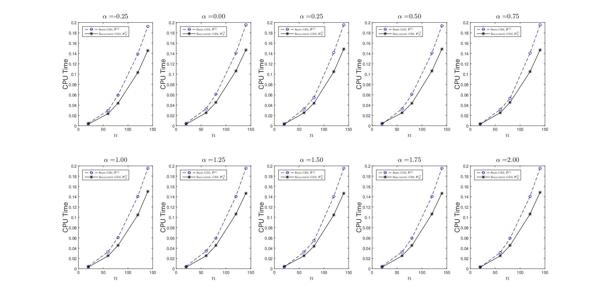
In this section, we discuss 1010 computational algorithms created to efficiently calculate the developed barycentric GIMs and quadratures and their optimal partners. We commence our discussion with Algorithms 1 and 2, which represent two simple and fast computational algorithms for the computation of the square barycentric GIM and its associated quadrature for the GG set of points; cf. Appendix A. We find that one of the major advantages of the established algorithms lies in the reduction of the operational cost required for calculating the GIM and quadrature. Indeed, the barycentric weights can be computed in O⁡(n)O(n) operations, whereas the LG points and quadrature weights, {xN,i(0.5),ϖN,i(0.5)}i=0N\left\{{x_{N,i}^{(0.5)},\varpi_{N,i}^{(0.5)}}\right\}_{i=0}^{N}, require O⁡(N)O(N) operations. Therefore, the computation of {pB,j,i(1)}i=0n\left\{{p_{B,j,i}^{(1)}}\right\}_{i=0}^{n} through Eq. (3.7) costs O⁡(N⋅n)O(N\cdot n) operations per point– the same cost required for the evaluation of the barycentric Gegenbauer quadrature through Eq. (3.6) for each point. This amounts to O⁡(N⋅n2)O\left(N\cdot n^{2}\right) for the construction of the barycentric GIM, 𝐏B(1){\mathbf{P}}_{B}^{(1)}. On the other hand, the evaluation of the Gegenbauer quadrature derived in [Elgindy and Smith-Miles (2013a), Theorem 2.1] in basis form requires O⁡(n2)O\left(n^{2}\right) operations per point while the cost of constructing the associated basis GIM rises up to O⁡(n3)O\left(n^{3}\right) operations. Figure 1 shows the average elapsed CPU time in 1010 runs required for the construction of the basis GIM, 𝐏^(1)\hat{\mathbf{P}}^{(1)}, derived by [Elgindy and Smith-Miles (2013a)] and the barycentric GIM, 𝐏B(1)\mathbf{P}_{B}^{(1)} using n=20,60,80,120,140n=20,60,80,120,140 points and α=−0.25​(0.25)​2\alpha=-0.25(0.25)2. Both GIMs were constructed in each case using the same inputs of GG points and quadrature weights, {xn,i(α),ϖn,i(α)}i=0n\left\{{x_{n,i}^{(\alpha)},\varpi_{n,i}^{(\alpha)}}\right\}_{i=0}^{n}. Clearly, the construction of 𝐏B(1)\mathbf{P}_{B}^{(1)} is faster than 𝐏^(1)\hat{\mathbf{P}}^{(1)}, and the gap grows wider for increasing values of nn.

Refer to caption
Figure 1: The average elapsed CPU time (in seconds) in 10 runs required for the construction of the basis GIM, 𝐏^(1)\hat{\mathbf{P}}^{(1)}, derived by [Elgindy and Smith-Miles (2013a)] and the barycentric GIM, 𝐏B(1)\mathbf{P}_{B}^{(1)} using n=20,60,80,120;140n=20,60,80,120;140, and α=−0.25​(0.25)​2\alpha=-0.25(0.25)2.

To analyze the errors of the barycentric and basis quadratures, we have conducted several numerical experiments on the three test functions f1​(x)=x20,f2​(x)=e−x2{f_{1}}(x)={x^{20}},\;{f_{2}}(x)={e^{-{x^{2}}}}, and f3​(x)=1/(1+25​x2){f_{3}}(x)=1/(1+25\,{x^{2}}), which were studied by [Elgindy and Smith-Miles (2013a)]. The absolute errors (AEs) obtained for {fi}i=13\{f_{i}\}_{i=1}^{3} are shown in Figures 2-4, where one can clearly verify that both quadratures share the same order of error for all {fi}i=13\{f_{i}\}_{i=1}^{3} with almost matched error values for the third test function, f3f_{3}.

Refer to caption
Refer to caption
Figure 2: The AEs of the barycentric and basis quadratures for f1f_{1} on [−1,1][-1,1] for α=−0.25​(0.25)​2\alpha=-0.25(0.25)2. Figures 2 and 2 show the results for n=20;80n=20;80, respectively.
Refer to caption
Refer to caption
Figure 3: The AEs of the barycentric and basis quadratures for f2f_{2} on [−1,1][-1,1] for α=−0.25​(0.25)​2\alpha=-0.25(0.25)2. Figures 3 and 3 show the results for n=20;80n=20;80, respectively.
Refer to caption
Refer to caption
Figure 4: The AEs of the barycentric and basis quadratures for f3f_{3} on [−1,1][-1,1] for α=−0.25​(0.25)​2\alpha=-0.25(0.25)2. Figures 4 and 4 show the results for n=20;80n=20;80, respectively.

Notice that both the CPU time and AEs were not reported for n=40,100,160n=40,100,160 as we observed that

|x^N,k(0.5)−xn,i(α)|≤εmach,\left|{\hat{x}_{N,k}^{(0.5)}-x_{n,i}^{(\alpha)}}\right|\leq\varepsilon_{\text{mach}}, (5.1)

for certain values of α\alpha, where

x^N,k(0.5)=12​((xn,j(α)+1)​xN,k(0.5)+xn,j(α)−1)​∀k,\hat{x}_{N,k}^{(0.5)}=\frac{1}{2}\left({\left({x_{n,j}^{(\alpha)}+1}\right){\mkern 1.0mu}x_{N,k}^{(0.5)}+x_{n,j}^{(\alpha)}-1}\right)\;\forall k, (5.2)

and εmach\varepsilon_{\text{mach}} denotes the machine precision that is approximately equals 2.2204×10−162.2204\times 10^{-16} in double precision arithmetic. For instance, we find that Eq. (5.1) is satisfied for k=25k=25 and i=33i=33 using 101101 GG points at α=1\alpha=1, where both x^50,25(0.5)\hat{x}_{50,25}^{(0.5)} and x100,33(1)x_{100,33}^{(1)} equals -0.5; thus overflow occurs. In fact, such a rare and unpleasant difficulty could happen whenever,

xN,k(0.5)=2​xn,i(α)−xn,j(α)+1xn,j(α)+1,x_{N,k}^{(0.5)}=\frac{{2x_{n,i}^{(\alpha)}-x_{n,j}^{(\alpha)}+1}}{{x_{n,j}^{(\alpha)}+1}}, (5.3)

for some i,j∈{0,…,n},k∈{0,…,N}i,j\in\{0,\ldots,n\},k\in\{0,\ldots,N\} in exact arithmetic, or

|1+xN,k(0.5)−2​(1+xn,i(α))1+xn,j(α)|≤ε​∀i,j;k,\left|{1+x_{N,k}^{(0.5)}-\frac{{2\left({1+x_{n,i}^{(\alpha)}}\right)}}{{1+x_{n,j}^{(\alpha)}}}}\right|\leq\varepsilon\;\forall i,j;k, (5.4)

in finite precision arithmetic, for some relatively small positive number ε\varepsilon. Therefore, a sufficient condition for constructing the barycentric GIM using Algorithm 1 is given by

|1+xN,k(0.5)−2​(1+xn,i(α))1+xn,j(α)|>ε​∀i,j;k.\left|{1+x_{N,k}^{(0.5)}-\frac{{2\left({1+x_{n,i}^{(\alpha)}}\right)}}{{1+x_{n,j}^{(\alpha)}}}}\right|>\varepsilon\;\forall i,j;k. (5.5)

We shall refer to the set,

𝔽B={(n,α):The Sufficient Condition (5.5) is always satisfied},\mathbb{F}_{B}=\left\{(n,\alpha):{\text{The Sufficient Condition }}\eqref{eq:rarecase3}\text{ is always satisfied}\right\}, (5.6)

by the “barycentric GIM feasible set.”

One approach to construct the barycentric GIM for (n,α)∉𝔽B(n,\alpha)\not\in\mathbb{F}_{B}, is to modify Algorithm 1 so that it accomplishes the fundamental property of Lagrange interpolating polynomials,

ℒB,n,i(α)(xN,k(0.5);−1,xn,j(α))=1,if x^N,k(0.5)=xn,i(α)∀i,k.\mathcal{L}_{B,n,i}^{(\alpha)}\left({x_{N,k}^{(0.5)};-1,x_{n,j}^{(\alpha)}}\right)=1,\quad{\text{if }}\hat{x}_{N,k}^{(0.5)}=x_{n,i}^{(\alpha)}\;\forall i,k. (5.7)

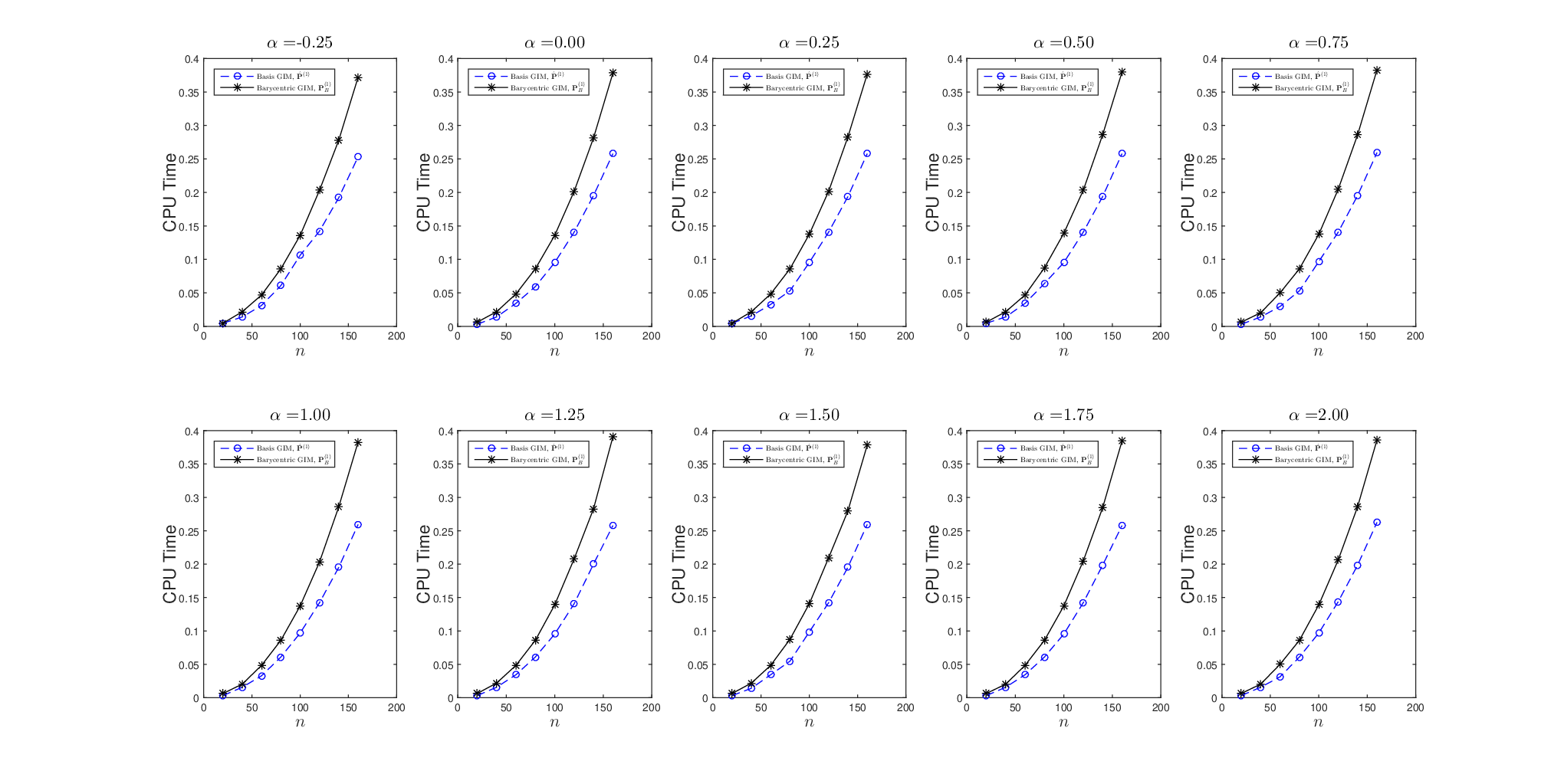
Algorithm 3 is a modification to Algorithm 1, which ensures the satisfaction of the Sufficient Condition (5.5); cf. Appendix A. The trick here is to set ℒB,n,i(α)​(xN,k(0.5),−1,xn,j(α))=1​∀i,j,k\mathcal{L}_{B,n,i}^{(\alpha)}\left({x_{N,k}^{(0.5)};-1,x_{n,j}^{(\alpha)}}\right)=1\;\forall i,j,k initially, and then update only the values of ℒB,n,i(α)​(xN,k(0.5),−1,xn,j(α))\mathcal{L}_{B,n,i}^{(\alpha)}\left({x_{N,k}^{(0.5)};-1,x_{n,j}^{(\alpha)}}\right) for which Condition (5.5) is satisfied. However, the result of such a modification casts its shadows on the time complexity required for constructing the barycentric GIM, 𝐏B(1){\mathbf{P}}_{B}^{(1)}. Indeed, Figure 5 shows that the time required for constructing the basis GIM, 𝐏^(1)\hat{\mathbf{P}}^{(1)}, derived by [Elgindy and Smith-Miles (2013a)] becomes shorter than that required for constructing 𝐏B(1){\mathbf{P}}_{B}^{(1)} using several values of nn and α\alpha.

Refer to caption
Figure 5: The average elapsed CPU time in 10 runs required for the construction of the basis GIM, 𝐏^(1)\hat{\mathbf{P}}^{(1)}, derived by [Elgindy and Smith-Miles (2013a)] and the barycentric GIM, 𝐏B(1)\mathbf{P}_{B}^{(1)}, using n=20​(20)​160n=20(20)160, and α=−0.25​(0.25)​2\alpha=-0.25(0.25)2.

Another approach to successfully construct the barycentric GIM for (n,α)∉𝔽B(n,\alpha)\not\in\mathbb{F}_{B} without applying Property (5.7) is to increase the value of NN if Condition (5.4) occurs before applying Algorithm 1; that is, we use instead an ⌈(n+3)/2⌉\left\lceil{(n+3)/2}\right\rceil-point LG quadrature for calculating the integrals

∫−11ℒB,n,i(α)​(t,−1,xn,j(α))​𝑑t,i,j=0,…,n.\int_{-1}^{1}{{\mathcal{L}}_{B,n,i}^{(\alpha)}\left({t;-1,x_{n,j}^{(\alpha)}}\right)\,dt},\quad i,j=0,\ldots,n. (5.8)

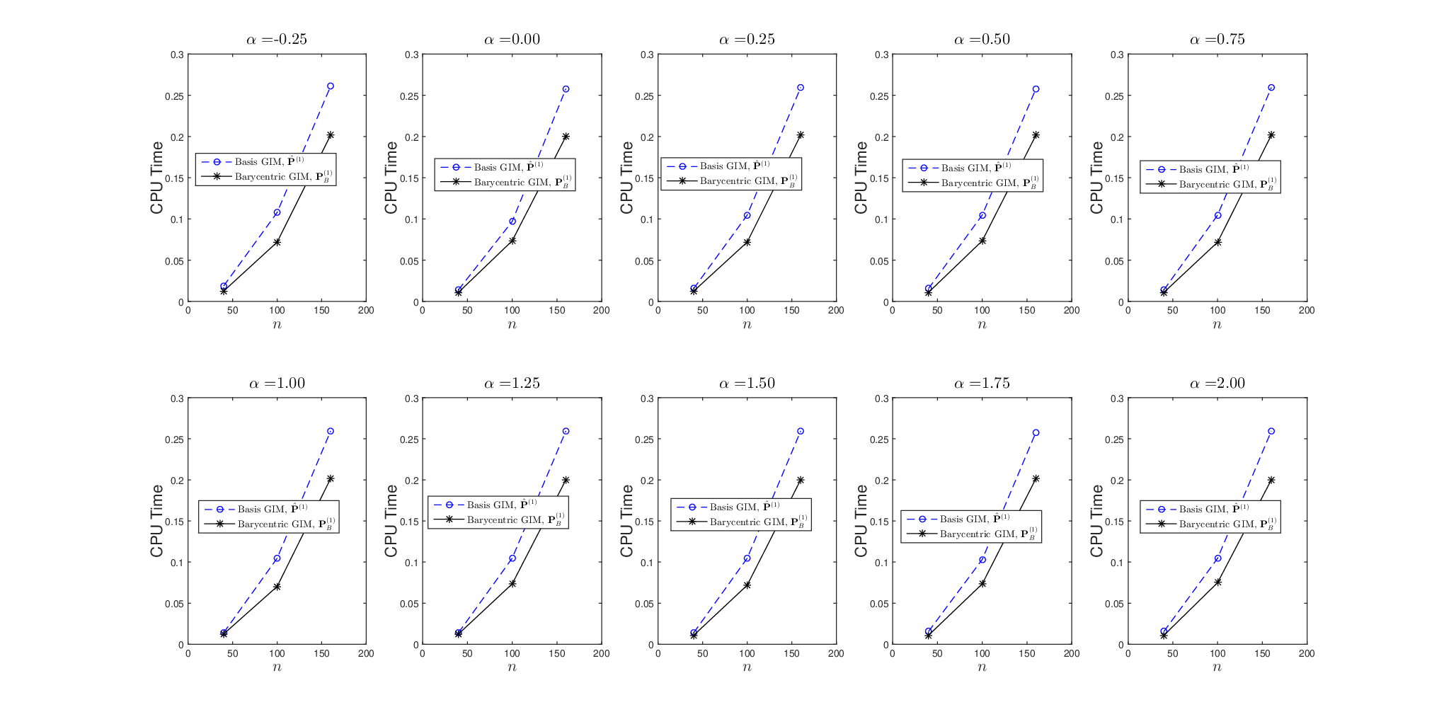
For instance, replacing NN with (N+1)(N+1) would change the values of {xN,k(0.5)}k=0N\{x_{N,k}^{(0.5)}\}_{k=0}^{N} with the possibility of fulfilling Condition (5.5) while exactly calculating the integrals (5.8) and retaining relatively lower computational cost. Algorithm 4 checks for the satisfaction of the Sufficient Condition (5.5); cf. Appendix A. Now running Algorithm 1 with the replacement of the statement N←⌈(n−1)/2⌉N\leftarrow\left\lceil{(n-1)/2}\right\rceil by N←⌈(n+1)/2⌉N\leftarrow\left\lceil{(n+1)/2}\right\rceil, retrieves the previous rapid construction of the barycentric GIM, 𝐏B(1){\mathbf{P}}_{B}^{(1)}, as verified by Figure 6.

Remark 5.1.

We checked the Sufficient Condition (5.5) using Algorithm 4 running on a Windows 10 64-bit operating system endowed with MATLAB V. R2014b (8.4.0.150421) in double precision arithmetic for n=1​(1)​100n=1(1)100, α=−0.4​(0.001)​2\alpha=-0.4(0.001)2, and ε=εmach\varepsilon=\varepsilon_{\text{mach}}. Failure to construct the barycentric GIM was only reported at α=1\alpha=1 for n=4​(12)​100n=4(12)100. Therefore, Gegenbauer collocation schemes can be carried out safely and efficiently using any of the aforementioned valid input data.
Refer to caption
Figure 6: The average elapsed CPU time in 10 runs required for the construction of the basis GIM, 𝐏^(1)\hat{\mathbf{P}}^{(1)}, derived by [Elgindy and Smith-Miles (2013a)] and the barycentric GIM, 𝐏B(1)\mathbf{P}_{B}^{(1)} using n=40,100;160n=40,100;160, and α=−0.25​(0.25)​2\alpha=-0.25(0.25)2.

5.1 Resolving boundary-value problems using the barycentric Gegenbauer quadrature

To solve the integral reformulations of differential problems provided with boundary conditions using Gauss collocation methods, one needs to approximate the integral of the unknown solution y⁡(x)y(x) on [−1,1][-1,1] using Gauss collocation points {xn,i(α)}i=0n⊂(−1,1)\{x_{n,i}^{(\alpha)}\}_{i=0}^{n}\subset(-1,1); that is the following integral is often required,

I=∫−11y⁡(x)​𝑑x.I=\int_{-1}^{1}{y(x)\,dx}. (5.9)

Since the barycentric GIM is in principal designed for the GG points, we cannot directly apply Algorithm 1 for evaluating II. Notice here that we cannot approximate II using a LG quadrature unless the collocation points are the LG points. Therefore, to consider the more general case, we shall modify Algorithm 1 to work for general GG points. At first, denote the point 11 by xn+1,j(α){x_{n+1,j}^{(\alpha)}}. Then Eqs. (3.7) can be written as follows:

pB,n+1,i(1)=∑k=0NϖN,k(0.5)ℒB,n,i(α)(xN,k(0.5);−1,xn,n+1(α)),i=0,…,n,p_{B,n+1,i}^{(1)}=\sum\limits_{k=0}^{N}{\;\varpi_{N,k}^{(0.5)}{\mkern 1.0mu}{\mathcal{L}}_{B,n,i}^{(\alpha)}\left({x_{N,k}^{(0.5)};-1,x_{n,n+1}^{(\alpha)}}\right)},\quad i=0,\ldots,n, (5.10)

where pB,n+1,i(1),i=0,…,np_{B,n+1,i}^{(1)},i=0,\ldots,n, are the elements of the additional row of the barycentric GIM, 𝐏B,n+1(1){\mathbf{P}}_{B,n+1}^{(1)}, corresponding to the point 11. Since x^N,k(0.5)=xN,k(0.5)​∀k\hat{x}_{N,k}^{(0.5)}=x_{N,k}^{(0.5)}\;\forall k in this case, the Sufficient Condition (5.5) is now simplified to

|xN,k(0.5)−xn,i(α)|>ε​∀i;k.\left|{x_{N,k}^{(0.5)}-x_{n,i}^{(\alpha)}}\right|>\varepsilon\;\forall i;k. (5.11)

Since n>N​∀n≥1n>N\;\forall n\geq 1, both LG and GG points share the zero value if both nn and NN are even. For instance, for n=4n=4, we find that x2,1(0.5)=x4,2(α)=0∀α>−1/2{x_{2,1}^{(0.5)}=x_{4,2}^{(\alpha)}}=0\,\forall\alpha>-1/2, and again overflow occurs. To overcome this issue we increase the number of LG points as discussed before so that NN is replaced with N+1N+1. This convenient technique is adopted in Algorithm 6; cf. Appendix A. Notice here that Algorithm 6 is implemented assuming 𝐏B(1){\mathbf{P}}_{B}^{(1)} for the GG collocation points is not required. If this is not the case, then the barycentric weights are already computed using Algorithm 1, and we can safely remove this partial procedure to gain more efficiency when calculating the row barycentric GIM corresponding to the point 11. This is depicted in Algorithm 7.

Remark 5.2.

The barycentric GIM can be slightly modified to work for any set of arbitrary points {xk}k=0n\{x_{k}\}_{k=0}^{n} by following Algorithm 8 in Appendix A.

5.2 Computational algorithms for the optimal barycentric GIM

Similar to the work of [Elgindy and Smith-Miles (2013a)], the computational cost of 𝐏O​B(1)\mathbf{P}_{OB}^{(1)} can be reduced significantly for arbitrarily symmetric set of points {xk}k=0n\{x_{k}\}_{k=0}^{n} if mm is even. Indeed, in this case, ∫−1xkGm+1(αk∗)​(x)​𝑑x=∫−1−xkGm+1(αk∗)​(x)​𝑑x​∀k\int_{-1}^{{x_{k}}}{G_{m+1}^{(\alpha_{k}^{*})}(x)\,dx}=\int_{-1}^{-{x_{k}}}{G_{m+1}^{(\alpha_{k}^{*})}(x)\,dx}\,\forall k; thus {αk∗}k=0⌈n/2⌉−1={αn−k∗}k=0⌈n/2⌉−1\left\{{\alpha_{k}^{*}}\right\}_{k=0}^{\left\lceil{n/2}\right\rceil-1}=\left\{{\alpha_{n-k}^{*}}\right\}_{k=0}^{\left\lceil{n/2}\right\rceil-1}, which implies that {zm,k,i(αk∗),ξm,k,i(αk∗)}i=0m={zm,n−k,i(αn−k∗),ξm,n−k,i(αn−k∗)}i=0m\left\{{z_{m,k,i}^{(\alpha_{k}^{*})},\xi_{m,k,i}^{(\alpha_{k}^{*})}}\right\}_{i=0}^{m}=\left\{{z_{m,n-k,i}^{(\alpha_{n-k}^{*})},\xi_{m,n-k,i}^{(\alpha_{n-k}^{*})}}\right\}_{i=0}^{m}, for k=0,…,⌈n/2⌉−1k=0,\ldots,{\left\lceil{n/2}\right\rceil}-1. Hence, {zm,k,i(αk∗),ξm,k,i(αk∗)}i=0m\left\{{z_{m,k,i}^{(\alpha_{k}^{*})},\xi_{m,k,i}^{(\alpha_{k}^{*})}}\right\}_{i=0}^{m} can be stored for the first (⌈n/2⌉−1)({\left\lceil{n/2}\right\rceil}-1) iterations, and invoked later in the next iterations. Algorithms 9 and 10 are two efficient algorithms for the construction of the optimal barycentric GIM for any non-symmetric/symmetric set of integration points, respectively; cf. Appendix A. For a large number of expansion terms, Chebyshev and Legendre quadratures often behave optimally as specified by the used error norm; cf. [Elgindy and Smith-Miles (2013a)]. Therefore, both algorithms provide the user with the flexibility to choose two parameter inputs mmaxm_{\max} and αa\alpha_{a} at which the algorithms construct the Chebyshev/Legendre quadratures instead. Moreover, the parameter input αb\alpha_{b} adds further stability to the algorithms in the occasions, where αk∗\alpha_{k}^{*} lies in the critical interval (−0.5,−0.5+ε)(-0.5,-0.5+\varepsilon). The parameter input rr is ideally chosen from the interval [1,2][1,2] to hamper the extrapolatory effect of the optimal Gegenbauer quadrature caused by the narrowing behavior of the Gegenbauer weight function for increasing values of α\alpha; cf. [Elgindy and Smith-Miles (2013a)]. For a non-symmetric set of integration nodes {xk}k=0n\{x_{k}\}_{k=0}^{n} with m≤mmax:mm\leq m_{\max}:m is even and 1∈{xk}k=0n1\in\{x_{k}\}_{k=0}^{n}, MM should be replaced with (M+1)(M+1) in Algorithm 9 if MM is even, as we discussed earlier. This procedure should also be carried out in Algorithm 10 for symmetric sets of integration nodes with m≤mmaxm\leq m_{\max} and 1∈{xk}k=0n1\in\{x_{k}\}_{k=0}^{n}, since mm is always an even integer in such cases.

Since Algorithms 9 and 10 work for any arbitrary set of nodes {xk}k=0n\{x_{k}\}_{k=0}^{n}, the Sufficient Condition (5.5) for m>mmaxm>m_{\max} now becomes

|xM,s(0.5)−1−xk+2​xm,i(αa)1+xk|>ε​∀i,s;k,\left|{x_{M,s}^{(0.5)}-\frac{{1-{x_{k}}+2x_{m,i}^{({\alpha_{a}})}}}{{1+{x_{k}}}}}\right|>\varepsilon\;\forall i,s;k, (5.12)

which can be checked using Algorithm 5. We refer to the set,

𝔽O​B,1(mmax)={(m,αa):m>mmax;the Sufficient Condition (5.12) is always satisfied},\mathbb{F}_{OB,1}^{(m_{\max})}=\left\{(m,\alpha_{a}):m>m_{\max};{\text{the Sufficient Condition }}\eqref{eq:rarecase3OB}\text{ is always satisfied}\right\}, (5.13)

by the “optimal barycentric GIM feasible set for m>mmaxm>m_{\max}.” It is important here to mention that in Gegenbauer collocation schemes, the dynamics is often enforced at the GG points; cf. [Elgindy and Smith-Miles (2013a), Elgindy and Smith-Miles (2013b), Elgindy (2016a), Elgindy, Smith-Miles, and Miller (2012), Elgindy and Smith-Miles (2013c)]. Therefore, the input set of integration nodes {xk}k=0n\{{x_{k}}\}_{k=0}^{n} in Algorithm 10 is frequently taken as the set of GG points {xn,k(α)}k=0n\{x_{n,k}^{(\alpha)}\}_{k=0}^{n}. Hence, the sufficient condition for constructing 𝐏O​B(1)\mathbf{P}_{OB}^{(1)} for m≤mmaxm\leq m_{\max} reads

|xM,s(0.5)−1−xn,k(α)+2​zm,k,i(αk∗)1+xn,k(α)|>ε​∀i,s;k.\left|{x_{M,s}^{(0.5)}-\frac{{1-x_{n,k}^{(\alpha)}+2\,z_{m,k,i}^{(\alpha_{k}^{*})}}}{{1+x_{n,k}^{(\alpha)}}}}\right|>\varepsilon\;\forall i,s;k. (5.14)

We refer to the set,

𝔽O​B,2(mmax)={(n,m,α):m≤mmax;the Sufficient Condition (5.14) is always satisfied},\mathbb{F}_{OB,2}^{(m_{\max})}=\left\{(n,m,\alpha):m\leq m_{\max};{\text{the Sufficient Condition }}\eqref{eq:rarecase3OBmlmmax}\text{ is always satisfied}\right\}, (5.15)

by the “optimal barycentric GIM feasible set for m≤mmaxm\leq m_{\max}.” The above argument implies that the set,

𝔽O​B(mmax)={𝔽O​B,1(mmax),m>mmax,𝔽O​B,2(mmax),m≤mmax,\mathbb{F}_{OB}^{({m_{\max}})}=\left\{\begin{array}[]{l}\mathbb{F}_{OB,1}^{({m_{\max}})},\quad m>{m_{\max}},\\ \mathbb{F}_{OB,2}^{({m_{\max}})},\quad m\leq{m_{\max}},\end{array}\right. (5.16)

is the optimal barycentric GIM feasible set.

Remark 5.3.

The phrase ‘If M=NM=N then set 𝐏=𝐏^\mathbf{P}=\hat{\mathbf{P}} with α=0.5\alpha=0.5;’ in [Elgindy and Smith-Miles (2013a), Algorithms 2.1 & 2.2] should be carried out with each iith-indexed GG point xix_{i} replaced with the corresponding arbitrary point while keeping the jjth-indexed GG points xjx_{j} the same. This should be straightforward and the implementation should follow that of Algorithm 8 in Appendix A. We have also noticed a typo in [Elgindy and Smith-Miles (2013a), Algorithm 2.2], where the phrase ‘NN is even’ in the input should be replaced with ‘MM is even.’ In turns, the condition ‘i≤N/2i\leq N/2’ in Step 4 should be correctly replaced with ‘i≤⌊N/2⌋i\leq\left\lfloor{N/2}\right\rfloor’ to cover both cases when NN is even or odd.

Remark 5.4.

Since most of the current state of the art software such as MATLAB are optimized for operations involving matrices and vectors, all of the proposed algorithms are vectorized to run much faster than the corresponding codes containing loops.

6 Numerical examples

In this section, we apply the developed barycentric GIMs and quadratures on three well-studied test examples with known exact solutions in the literature. Comparisons with other competitive numerical schemes are presented to assess the accuracy and efficiency of the current work. The numerical experiments were conducted on a personal laptop equipped with an Intel(R) Core(TM) i7-2670QM CPU with 2.20GHz speed running on a Windows 10 64-bit operating system.

Example 1

Consider the following Fredholm integro-differential equation:

y′​(x)−y⁡(x)−∫01es​x​y​(s)​𝑑s=1−ex+1x+1,y⁡(0)=1,y^{\prime}(x)-y(x)-\int_{0}^{1}{{e^{sx}}\;y(s)\;ds}=\frac{{1-{e^{x+1}}}}{{x+1}},\quad y(0)=1, (6.1)

with the exact solution y⁡(x)=exy(x)=e^{x}. This problem was previously solved by [Elgindy and Smith-Miles (2013b)] using a hybrid Gegenbauer integration method (HGIM). Following the numerical scheme developed by [Elgindy and Smith-Miles (2013b)] together with the obtained barycentric GIMs results in the following algebraic system of linear equations:

wj−∑i=0n(pB,j,i(1)+∑k=0npB,n+1,i(1)pB,j,k(1)exn,k(α)​xn,i(α))wi−∑i=0mpO​B,j,i(1)rj,i−1=0,j=0,…,n,{w_{j}}-\sum\limits_{i=0}^{n}{\left({p_{B,j,i}^{(1)}+\sum\limits_{k=0}^{n}{p_{B,n+1,i}^{(1)}p_{B,j,k}^{(1)}{e^{x_{n,k}^{(\alpha)}x_{n,i}^{(\alpha)}}}}}\right){\mkern 1.0mu}{w_{i}}-\sum\limits_{i=0}^{m}{p_{OB,j,i}^{(1)}\;{r_{j,i}}}-1=0},\quad j=0,\ldots,n, (6.2)

where wj≈y⁡(xn,j(α))​∀j;r⁡(x)=(1−ex+1)/(x+1).{w_{j}}\approx y\left(x_{n,j}^{(\alpha)}\right)\,\forall j;r(x)=\left(1-{e^{x+1}}\right)/(x+1). We refer to the present method by the hybrid barycentric Gegenbauer integration method (HBGIM). We implemented the developed algorithms for the set of feasible 33-tuples {(10,14,α)}α=−0.4​(0.1)1\{(10,14,\alpha)\}_{\alpha=-0.4(0.1)}^{1} ⊂𝔽O​B(20)\subset\mathbb{F}_{OB}^{(20)}. The resulting algebraic linear system of equations were solved using MATLAB “mldivide” Algorithm provided with MATLAB V. R2014b (8.4.0.150421). Figure 7 shows the maximum absolute errors (MAEs) of the present method. As can be observed from the results, the maxα=−0.4:0.1:1MAE\max_{\alpha=-0.4:0.1:1}\text{MAE} of the present method is about 9.948×10−149.948\times 10^{-14} obtained at α=1\alpha=1 versus approximately 4.201×10−134.201\times 10^{-13} for the HGIM obtained at α=−0.4\alpha=-0.4. The best MAE ≈5.329×10⁻¹⁵\approx 5.329\times 10^{-15} was obtained at α=0.7\alpha=0.7 in 0.0170.017 seconds. The reported 22-norm condition number, κ2{\kappa_{2}}, of the linear system is approximately bounded by 35.27≤κ2≤42.87​∀α35.27\leq{\kappa_{2}}\leq 42.87\;\forall\alpha.

Refer to caption
Figure 7: The figure shows the MAEs of the HGIM versus the HBGIM for the set of feasible 33-tuples {(10,14,α)}α=−0.4​(0.1)1\{(10,14,\alpha)\}_{\alpha=-0.4(0.1)}^{1} ⊂𝔽O​B(20)\subset\mathbb{F}_{OB}^{(20)}.

Example 2

Consider the following nonlinear boundary value problem:

−cα​α​(∫01u⁡(t)​𝑑t)​u′′​(x)+u5​(x)=0,  0<x<1,-{c_{\alpha}}\alpha\left({\int_{0}^{1}{u(t)\,dt}}\right)\,u^{\prime\prime}(x)+{u^{5}}(x)=0,\;\;0<x<1, (6.3)

such that u(0)=1,u(1)=2/2,cα=4/(3α(22−2));α(q)=1/q∀q>0.u(0)=1,u(1)=\sqrt{2}/2,{c_{\alpha}}=4/\left({3\,\alpha\left({2\sqrt{2}-2}\right)}\right);\alpha(q)=1/q\,\forall q>0. The exact solution is u⁡(x)=1/1+xu(x)=1/\sqrt{1+x} [Themistoclakis and Vecchio (2015)]. Notice here that the coefficient of the second derivative of the unknown solution uu depends upon the integral of uu itself, which in turn depends on the whole solution domain [0,1][0,1] rather than on a single point. Therefore, the boundary value problem is classified as a “nonlocal” nonlinear problem. This problem was studied by [Themistoclakis and Vecchio (2015)] and was solved using an iterative scheme (IS). The present HBGIM results in the following nonlinear algebraic system of equations:

PB(2)​U(5)−PB,n+1(2)​U(5)​X+[4​(4−3​2)​X−8​(2−1)​(U−1)]⊘(3​PB,n+1(1)​U),P_{B}^{(2)}{U^{(5)}}-P_{B,n+1}^{(2)}{U^{(5)}}X+\left[{4\left({4-3\sqrt{2}}\right)X-8\left({\sqrt{2}-1}\right)\left({U-1}\right)}\right]\oslash\left({3P_{B,n+1}^{(1)}U}\right), (6.4)

where U=[U0,U1,…,Un]T≈[u⁡(xn,0(α)),u⁡(xn,1(α)),…,u⁡(xn,n(α))]T,X=[xn,0(α),xn,1(α),…,xn,n(α)]T;U={\left[{{U_{0}},{U_{1}},\ldots,{U_{n}}}\right]^{T}}\approx{\left[{u\left({x_{n,0}^{(\alpha)}}\right),u\left({x_{n,1}^{(\alpha)}}\right),\ldots,u\left({x_{n,n}^{(\alpha)}}\right)}\right]^{T}},X={\left[{x_{n,0}^{(\alpha)},x_{n,1}^{(\alpha)},\ldots,x_{n,n}^{(\alpha)}}\right]^{T}};

U(5)=U∘U​…∘U⏟5−times,{U^{(5)}}=\underbrace{U\circ U\ldots\circ U}_{5-{\text{times}}},

∘\circ and ⊘\oslash denote the Hadamard product and division, respectively. We implemented the developed algorithms for the set of feasible pairs {(n,α):n=6,7,9;α=−0.4(0.1)1}⊂𝔽B\{(n,\alpha):n=6,7,9;\alpha=-0.4(0.1)1\}\subset\mathbb{F}_{B}. The nonlinear system (6.4) was solved using MATLAB “fsolve” solver with “TolX” set at εmach\varepsilon_{\text{mach}}. Figure 8 shows the MAEs of the present method while Figure 9 shows the number of correct digits cdn:=−log10⁡[max0≤i≤n⁡|u⁡(xi)−Ui|]{\text{c}}{{\text{d}}_{n}}:=-{\log_{10}}\left[{{{\max}_{0\leq i\leq n}}\left|{u({x_{i}})-{U_{i}}}\right|}\right] obtained in each case. Clearly, the present numerical scheme achieves a very rapid convergence rate using relatively small number of barycentric quadratures terms. For instance, the IS of [Themistoclakis and Vecchio (2015)] requires 257257 points to obtain 66 correct digits versus only 1010 GG points to achieve a larger number of correct digits for the present method with an elapsed time of about 0.010.01 seconds for all experimental values of α\alpha. Both numerical tests confirm the efficiency of the proposed numerical schemes.

Refer to caption
Figure 8: The MAEs of the HBGIM for {(n,α):n=6,7,9;α=−0.4(0.1)1}⊂𝔽B\{(n,\alpha):n=6,7,9;\alpha=-0.4(0.1)1\}\subset\mathbb{F}_{B}.
Refer to caption
Figure 9: The cdn for the HBGIM and the IS of [Themistoclakis and Vecchio (2015)].

Example 3

Consider the following second-order one-dimensional hyperbolic telegraph equation,

ut​t​(x,t)+2​π2​ut​(x,t)+π2​u​(x,t)=ux​x​(x,t)+e−t​sin⁡(π​x),0≤x≤1,t>0,{u_{tt}}(x,t)+2{\pi^{2}}{u_{t}}(x,t)+{\pi^{2}}u(x,t)={u_{xx}}(x,t)+{e^{-t}}\sin(\pi x),\quad 0\leq x\leq 1,t>0, (6.5)

provided with the initial conditions,

u⁡(x,0)\displaystyle u(x,0) =sin⁡(π​x),\displaystyle=\sin(\pi x), (6.6)
ut​(x,0)\displaystyle{u_{t}}(x,0) =−sin⁡(π​x),\displaystyle=-\sin(\pi x), (6.7)

and the following Dirichlet boundary conditions,

u⁡(0,t)=0;\displaystyle u(0,t)=0; (6.8)
u⁡(1,t)=0.\displaystyle u(1,t)=0. (6.9)

The exact solution of the above problem is u⁡(x,t)=e−t​sin⁡(π​x)u(x,t)={e^{-t}}\sin(\pi x) [Luo and Du (2013)]. We solved the problem using the numerical scheme developed by [Elgindy (2016a)] together with the obtained barycentric GIMs. The developed algorithms were carried out using the feasible 33-tuple (8,8,0)∈𝔽O​B(20)(8,8,0)\in\mathbb{F}_{OB}^{(20)}. The plots of the exact solution, its bivariate shifted Gegenbauer interpolant Pn,n​u​(x,t){P_{n,n}}u(x,t) (see [Elgindy (2016a)]), and the absolute error function

En,n​(x,t)=|u⁡(x,t)−Pn,n​u​(x,t)|,(x,t)∈D1,12,{E}_{n,n}(x,t)=\left|u(x,t)-{P_{n,n}}u(x,t)\right|,\quad(x,t)\in D_{1,1}^{2}, (6.10)

are shown in Figure 10, where D1,12=[0,1]×[0,1]D_{1,1}^{2}=[0,1]\times[0,1]. A comparison with [Luo and Du (2013)]’s fourth-order method based on cubic Hermite interpolation [Luo and Du (2013)] and the present method is also shown in Table 1. The plots and the numerical comparisons show the power of the present method as proven in the recognized rapid convergence rates and the produced errors with very small magnitudes using relatively small number of expansion terms. For instance, [Luo and Du (2013)]’s fourth-order method [Luo and Du (2013)] yields a MAE of order 10−0810^{-08} using 49×4949\times 49 collocation points in both directions. Conversely, a MAE of order 10−0910^{-09} is achieved by the present method using only 11×1111\times 11 collocation points.

Refer to caption
Figure 10: The numerical simulation of the present method on Example 3. The figure shows the plots of the exact solution u⁡(x,t)u(x,t) on D1,12D_{1,1}^{2} (upper left), its approximation P8,8​u​(x,t)P_{8,8}u(x,t) (upper right), the absolute error function E8,8​(x,t){E}_{8,8}(x,t) (lower left), and its values at the final time, E8,8​(x,1){E}_{8,8}(x,1) (lower right). The barycentric matrix and its optimal partner are both square of size 99. The plots were generated using 100100 linearly spaced nodes in the xx- and tt-directions from 00 to 11.
Example 3
[Luo and Du (2013)]’s method [Luo and Du (2013)] Present method
(h)/(M​A​E);k=1/48(h)/(MAE);k=1/48 (n)/(M​A​E)(n)/(MAE)
(1/12)/(3.702×10−06)(1/12)/(3.702\times 10^{-06}) (8)/(3.303×10−07)(8)/(3.303\times 10^{-07})
(1/24)/(2.310×10−07)(1/24)/(2.310\times 10^{-07}) (10)/(1.596×10−09)(10)/(1.596\times 10^{-09})
(1/48)/(1.451×10−08)(1/48)/(1.451\times 10^{-08}) (12)/(5.145×10−12)(12)/(5.145\times 10^{-12})
(1/96)/(9.952×10−10)(1/96)/(9.952\times 10^{-10}) (14)/(1.849×10−14)(14)/(1.849\times 10^{-14})
Table 1: A comparison of Example 3 between [Luo and Du (2013)]’s fourth-order method [Luo and Du (2013)] and the current method. The table lists the MAEs at t=1t=1. The results of [Luo and Du (2013)]’s method [Luo and Du (2013)] are quoted from Ref. [Luo and Du (2013)].

7 Conclusion and discussion

Novel GIMs and quadratures are developed based on the barycentric representation of Lagrange interpolating polynomials and the explicit barycentric weights for the GG points. The established GIMs and quadratures were optimized following the method of [Elgindy and Smith-Miles (2013a)]. The present numerical scheme leads to a reduction in the computational cost and time complexity while preserving the order of accuracy achieved by [Elgindy and Smith-Miles (2013a)]. The proposed HBGIM is a stable numerical scheme, which generally leads to well-conditioned systems. The numerical experiments confirm the stability, high-order accuracy, and efficiency of the proposed HBGIM and developed computational algorithms. The presented algorithms and numerical scheme provide easy yet strong numerical tools, which can be effectively carried out for the solution of a wide variety of problems. For instance, the current work laid the foundation of the exponentially-convergent numerical method of [Elgindy (2016c)] for solving optimal control problems governed by parabolic distributed parameter systems, and was the crucial element in deriving a high-order adaptive spectral element algorithm for solving general nonlinear optimal control problems exhibiting smooth/nonsmooth solutions using composite shifted Gegenbauer grids; cf. [Elgindy (2016b)]. Other possible future directions may include the extension of the current work to handle problems in multiple-space dimensions and the development of sparse/banded integration matrices.

8 Acknowledgments

I would like to express my deepest gratitude to the editor for carefully handling the article, and the anonymous reviewers for their careful reading, constructive comments, and useful suggestions, which shaped the article into its final form.

Appendix A Pseudocodes for the developed computational algorithms

Algorithm 1 Construction of the barycentric GIM for the GG set of integration points
0:  Positive integer nn; the set of GG points and quadrature weights, {xn,i(α),ϖn,i(α)}i=0n\left\{{x_{n,i}^{(\alpha)},\varpi_{n,i}^{(\alpha)}}\right\}_{i=0}^{n}.
 ξn,i(α)←(−1)isin(cos−1(xn,i(α)))ϖn,i(α),i=0,…,n.\xi_{n,i}^{(\alpha)}\leftarrow{(-1)^{i}}{\mkern 1.0mu}\sin\left({{{\cos}^{-1}}\left({x_{n,i}^{(\alpha)}}\right)}\right)\sqrt{\varpi_{n,i}^{(\alpha)}},\quad i=0,\ldots,n.
 N←⌈(n−1)/2⌉N\leftarrow\left\lceil{(n-1)/2}\right\rceil.
 Calculate the set of LG points and quadrature weights, {xN,i(0.5),ϖN,i(0.5)}i=0N\left\{{x_{N,i}^{(0.5)},\varpi_{N,i}^{(0.5)}}\right\}_{i=0}^{N}.
 𝐏B(1)←𝐎{\mathbf{P}}_{B}^{(1)}\leftarrow{\mathbf{O}}.
 for j=0j=0 to nn do
  x^N,k(0.5)←((xn,j(α)+1)xN,k(0.5)+xn,j(α)−1)/2,k=0,…,N\hat{x}_{N,k}^{(0.5)}\leftarrow\left({\left({x_{n,j}^{(\alpha)}+1}\right)x_{N,k}^{(0.5)}+x_{n,j}^{(\alpha)}-1}\right)/2,\quad k=0,\ldots,N.
  for k=0k=0 to NN do
   μi←ξn,i(α)/(x^N,k(0.5)−xn,i(α)),i=0,…,n.{\mu_{i}}\leftarrow\xi_{n,i}^{(\alpha)}/\left({\hat{x}_{N,k}^{(0.5)}-x_{n,i}^{(\alpha)}}\right),\quad i=0,\ldots,n.ν←∑i=0nμi\nu\leftarrow\sum\nolimits_{i=0}^{n}{{\mu_{i}}}.pB,j,i←pB,j,i+ϖN,k(0.5)μi/ν,i=0,…,n.{p_{B,j,i}}\leftarrow{p_{B,j,i}}+\varpi_{N,k}^{(0.5)}{\mu_{i}}/\nu,\quad i=0,\ldots,n.
  end for
  pB,j,i←(xn,j(α)+1)pB,j,i/2,i=0,…,n.{p_{B,j,i}}\leftarrow\left({x_{n,j}^{(\alpha)}+1}\right){p_{B,j,i}}/2,\quad i=0,\ldots,n.
 end for
 return 𝐏B(1){\mathbf{P}}_{B}^{(1)}
Algorithm 2 Calculation of the barycentric Gegenbauer quadrature for the GG set of integration points
0:  Positive integer nn; the set of GG points and quadrature weights, {xn,i(α),ϖn,i(α)}i=0n\left\{{x_{n,i}^{(\alpha)},\varpi_{n,i}^{(\alpha)}}\right\}_{i=0}^{n}; real-valued function ff.
 Construct 𝐏B(1){\mathbf{P}}_{B}^{(1)} using Algorithm 1.
 𝐈n(α)←𝐏B(1)⋅(fn,0(α),fn,1(α),…,fn,n(α))T{\mathbf{I}}_{n}^{(\alpha)}\leftarrow{\mathbf{P}}_{B}^{(1)}\cdot{\left({f_{n,0}^{(\alpha)},f_{n,1}^{(\alpha)},\ldots,f_{n,n}^{(\alpha)}}\right)^{T}}.
 return 𝐈n(α){\mathbf{I}}_{n}^{(\alpha)}
Algorithm 3 Modified construction of the barycentric GIM for the GG set of integration points
0:  Positive integer nn; the set of GG points and quadrature weights, {xn,i(α),ϖn,i(α)}i=0n\left\{{x_{n,i}^{(\alpha)},\varpi_{n,i}^{(\alpha)}}\right\}_{i=0}^{n}; relatively small positive number ε\varepsilon.
 ξn,i(α)←(−1)isin(cos−1(xn,i(α)))ϖn,i(α),i=0,…,n.\xi_{n,i}^{(\alpha)}\leftarrow{(-1)^{i}}{\mkern 1.0mu}\sin\left({{{\cos}^{-1}}\left({x_{n,i}^{(\alpha)}}\right)}\right)\sqrt{\varpi_{n,i}^{(\alpha)}},\quad i=0,\ldots,n.
 N←⌈(n−1)/2⌉N\leftarrow\left\lceil{(n-1)/2}\right\rceil.
 Calculate the set of LG points and quadrature weights, {xN,i(0.5),ϖN,i(0.5)}i=0N\left\{{x_{N,i}^{(0.5)},\varpi_{N,i}^{(0.5)}}\right\}_{i=0}^{N}.
 𝐏B(1)←𝐎{\mathbf{P}}_{B}^{(1)}\leftarrow{\mathbf{O}}
 Li←1,i=0,…,nL_{i}\leftarrow 1,\quad i=0,\ldots,n.
 for j=0j=0 to nn do
  x^N,k(0.5)←((xn,j(α)+1)xN,k(0.5)+xn,j(α)−1)/2,k=0,…,N\hat{x}_{N,k}^{(0.5)}\leftarrow\left({\left({x_{n,j}^{(\alpha)}+1}\right)x_{N,k}^{(0.5)}+x_{n,j}^{(\alpha)}-1}\right)/2,\quad k=0,\ldots,N.
  for k=0k=0 to NN do
   di=(x^N,k(0.5)−xn,i(α)),i=0,…,n.{d_{i}}=\left({\hat{x}_{N,k}^{(0.5)}-x_{n,i}^{(\alpha)}}\right),\quad i=0,\ldots,n.I←{i:|di|>ε}.I\leftarrow\left\{{i:\;\left|{{d_{i}}}\right|>\varepsilon}\right\}.μl←ξn,l(α)/dl,l∈I.{\mu_{l}}\leftarrow\xi_{n,l}^{(\alpha)}/d_{l},\quad l\in I.ν←∑l=0ℵ0μl\nu\leftarrow\sum\nolimits_{l=0}^{\aleph_{0}}{{\mu_{l}}}. {ℵ0\aleph_{0} denotes the cardinal number of II.}Ll=μl/ν,l∈I.{L_{l}}={\mu_{l}}/\nu,\quad l\in I.pB,j,i←pB,j,i+ϖN,k(0.5)Li,i=0,…,n.{p_{B,j,i}}\leftarrow{p_{B,j,i}}+\varpi_{N,k}^{(0.5)}{L_{i}},\quad i=0,\ldots,n.Ll=1,l∈I.{L_{l}}=1,\quad l\in I.
  end for
  pB,j,i←(xn,j(α)+1)pB,j,i/2,i=0,…,n.{p_{B,j,i}}\leftarrow\left({x_{n,j}^{(\alpha)}+1}\right){p_{B,j,i}}/2,\quad i=0,\ldots,n.
 end for
 return 𝐏B(1){\mathbf{P}}_{B}^{(1)}
Algorithm 4 Testing the sufficient condition (5.5) for the construction of the barycentric GIM for the GG set of integration points
0:  Positive integer nn; the set of GG points, {xn,i(α),}i=0n\left\{x_{n,i}^{(\alpha)},\right\}_{i=0}^{n}; relatively small positive number ε\varepsilon.
 N←⌈(n−1)/2⌉N\leftarrow\left\lceil{(n-1)/2}\right\rceil.
 Calculate the set of LG points, {xN,i(0.5)}i=0N\left\{x_{N,i}^{(0.5)}\right\}_{i=0}^{N}.
 for j=0j=0 to nn do
  for k=0k=0 to NN do
   J←{Ji:Ji={1,|1+xN,k(0.5)−2​(1+xn,i(α))/(1+xn,j(α))|≤ε,0,otherwise,i=0,…,n}.J\leftarrow\left\{{{J_{i}}:{J_{i}}=\left\{\begin{array}[]{l}1,\quad\left|{1+x_{N,k}^{(0.5)}-2\left({1+x_{n,i}^{(\alpha)}}\right)/\left({1+x_{n,j}^{(\alpha)}}\right)}\right|\leq\varepsilon,\\ 0,\quad{\text{otherwise,}}\end{array}\right.i=0,\ldots,n}\right\}.
   if ∑i=0ℵ0Ji>0\sum\nolimits_{i=0}^{{\aleph_{0}}}{{J_{i}}}>0 then {ℵ0\aleph_{0} denotes the cardinal number of JJ.}
    
    return “The test fails.”
   end if
  end for
 end for
 return “The test succeeds.”
Algorithm 5 Testing the sufficient condition for the construction of the optimal barycentric GIM for m>mmaxm>m_{\max}
0:  Positive integers m,lm,l; the set of GG points, {xm,i(αa),}i=0m\left\{x_{m,i}^{(\alpha_{a})},\right\}_{i=0}^{m}; the set of integration points, {xk}k=0l\{x_{k}\}_{k=0}^{l}; relatively small positive number ε\varepsilon.
 M←⌈(m−1)/2⌉M\leftarrow\left\lceil{(m-1)/2}\right\rceil.
 Calculate the set of LG points, {xM,s(0.5)}s=0M\left\{x_{M,s}^{(0.5)}\right\}_{s=0}^{M}.
 for i=0i=0 to mm do
  for s=0s=0 to MM do
   J←{Jk:Jk={1,|xM,s(0.5)−(1−xk+2​xm,i(αa))/(1+xk)|≤ε,0,otherwise,k=0,…,l}.J\leftarrow\left\{{{J_{k}}:{J_{k}}=\left\{{\begin{array}[]{*{20}{l}}{1,\quad\left|{x_{M,s}^{(0.5)}-({1-{x_{k}}+2x_{m,i}^{({\alpha_{a}})}})/({{1+{x_{k}}}})}\right|\leq\varepsilon,}\\ {0,\quad{\text{otherwise,}}}\end{array}}\right.k=0,\ldots,l}\right\}.
   if ∑k=0ℵ0Jk>0\sum\nolimits_{k=0}^{{\aleph_{0}}}{{J_{k}}}>0 then {ℵ0\aleph_{0} denotes the cardinal number of JJ.}
    
    return “The test fails.”
   end if
  end for
 end for
 return “The test succeeds.”
Algorithm 6 Construction of a row barycentric GIM corresponding to the point 11
0:  Positive integer nn; the set of GG points and quadrature weights, {xn,i(α),ϖn,i(α)}i=0n\left\{{x_{n,i}^{(\alpha)},\varpi_{n,i}^{(\alpha)}}\right\}_{i=0}^{n}.
0:  𝐏B(1){\mathbf{P}}_{B}^{(1)} is not required.
 ξn,i(α)←(−1)isin(cos−1(xn,i(α)))ϖn,i(α),i=0,…,n.\xi_{n,i}^{(\alpha)}\leftarrow{(-1)^{i}}{\mkern 1.0mu}\sin\left({{{\cos}^{-1}}\left({x_{n,i}^{(\alpha)}}\right)}\right)\sqrt{\varpi_{n,i}^{(\alpha)}},\quad i=0,\ldots,n.
 N←⌈(n−1)/2⌉N\leftarrow\left\lceil{(n-1)/2}\right\rceil.
 if mod​(n,2)=0∧mod​(N,2)=0{\text{mod}}(n,2)=0\;\wedge\;\text{mod}(N,2)=0 then
  N←N+1.N\leftarrow N+1.
 end if
 pB,n+1,i←0,i=0,…,n.{p_{B,n+1,i}}\leftarrow 0,\quad i=0,\ldots,n.Calculate the set of LG points and quadrature weights, {xN,i(0.5),ϖN,i(0.5)}i=0N\left\{{x_{N,i}^{(0.5)},\varpi_{N,i}^{(0.5)}}\right\}_{i=0}^{N}.
 for k=0k=0 to NN do
  μi←ξn,i(α)/(xN,k(0.5)−xn,i(α)),i=0,…,n.{\mu_{i}}\leftarrow\xi_{n,i}^{(\alpha)}/\left({x_{N,k}^{(0.5)}-x_{n,i}^{(\alpha)}}\right),\quad i=0,\ldots,n.ν←∑i=0nμi\nu\leftarrow\sum\nolimits_{i=0}^{n}{{\mu_{i}}}.pB,n+1,i←pB,n+1,i+ϖN,k(0.5)μi/ν,i=0,…,n.{p_{B,n+1,i}}\leftarrow{p_{B,n+1,i}}+\varpi_{N,k}^{(0.5)}{\mu_{i}}/\nu,\quad i=0,\ldots,n.
 end for
 return 𝐏B,n+1(1){\mathbf{P}}_{B,n+1}^{(1)}
Algorithm 7 Modified construction of a row barycentric GIM corresponding to the point 11
0:  Positive integer nn; the set of GG points and barycentric weights, {xn,i(α),ξn,i(α)}i=0n\left\{{x_{n,i}^{(\alpha)},\xi_{n,i}^{(\alpha)}}\right\}_{i=0}^{n}.
0:  𝐏B(1){\mathbf{P}}_{B}^{(1)} is already calculated.
 N←⌈(n−1)/2⌉N\leftarrow\left\lceil{(n-1)/2}\right\rceil.
 if mod​(n,2)=0∧mod​(N,2)=0{\text{mod}}(n,2)=0\;\wedge\;\text{mod}(N,2)=0 then
  N←N+1.N\leftarrow N+1.
 end if
 pB,n+1,i←0,i=0,…,n.{p_{B,n+1,i}}\leftarrow 0,\quad i=0,\ldots,n.Calculate the set of LG points and quadrature weights, {xN,i(0.5),ϖN,i(0.5)}i=0N\left\{{x_{N,i}^{(0.5)},\varpi_{N,i}^{(0.5)}}\right\}_{i=0}^{N}.
 for k=0k=0 to NN do
  μi←ξn,i(α)/(xN,k(0.5)−xn,i(α)),i=0,…,n.{\mu_{i}}\leftarrow\xi_{n,i}^{(\alpha)}/\left({x_{N,k}^{(0.5)}-x_{n,i}^{(\alpha)}}\right),\quad i=0,\ldots,n.ν←∑i=0nμi\nu\leftarrow\sum\nolimits_{i=0}^{n}{{\mu_{i}}}.pB,n+1,i←pB,n+1,i+ϖN,k(0.5)μi/ν,i=0,…,n.{p_{B,n+1,i}}\leftarrow{p_{B,n+1,i}}+\varpi_{N,k}^{(0.5)}{\mu_{i}}/\nu,\quad i=0,\ldots,n.
 end for
 return 𝐏B,n+1(1){\mathbf{P}}_{B,n+1}^{(1)}
Algorithm 8 Construction of the barycentric GIM for an arbitrary set of integration points
0:  Positive integers n,mn,m; the set of GG points and quadrature weights, {xn,i(α),ϖn,i(α)}i=0n\left\{{x_{n,i}^{(\alpha)},\varpi_{n,i}^{(\alpha)}}\right\}_{i=0}^{n}; the set of the integration nodes {xk}k=0m\{{x_{k}}\}_{k=0}^{m}.
 ξn,i(α)←(−1)isin(cos−1(xn,i(α)))ϖn,i(α),i=0,…,n.\xi_{n,i}^{(\alpha)}\leftarrow{(-1)^{i}}{\mkern 1.0mu}\sin\left({{{\cos}^{-1}}\left({x_{n,i}^{(\alpha)}}\right)}\right)\sqrt{\varpi_{n,i}^{(\alpha)}},\quad i=0,\ldots,n.
 N←⌈(n−1)/2⌉N\leftarrow\left\lceil{(n-1)/2}\right\rceil.
 Calculate the set of LG points and quadrature weights, {xN,i(0.5),ϖN,i(0.5)}i=0N\left\{{x_{N,i}^{(0.5)},\varpi_{N,i}^{(0.5)}}\right\}_{i=0}^{N}.
 𝐏B(1)←𝐎{\mathbf{P}}_{B}^{(1)}\leftarrow{\mathbf{O}}. {𝐎∈ℝ(m+1)×(n+1){\mathbf{O}}\in\mathbb{R}^{(m+1)\times(n+1)}}
 for j=0j=0 to mm do
  x^N,k(0.5)←((xj+1)xN,k(0.5)+xj−1)/2,k=0,…,N\hat{x}_{N,k}^{(0.5)}\leftarrow\left({\left({x_{j}+1}\right)x_{N,k}^{(0.5)}+x_{j}-1}\right)/2,\quad k=0,\ldots,N.
  for k=0k=0 to NN do
   μi←ξn,i(α)/(x^N,k(0.5)−xn,i(α)),i=0,…,n.{\mu_{i}}\leftarrow\xi_{n,i}^{(\alpha)}/\left({\hat{x}_{N,k}^{(0.5)}-x_{n,i}^{(\alpha)}}\right),\quad i=0,\ldots,n.ν←∑i=0nμi\nu\leftarrow\sum\nolimits_{i=0}^{n}{{\mu_{i}}}.pB,j,i←pB,j,i+ϖN,k(0.5)μi/ν,i=0,…,n.{p_{B,j,i}}\leftarrow{p_{B,j,i}}+\varpi_{N,k}^{(0.5)}{\mu_{i}}/\nu,\quad i=0,\ldots,n.
  end for
  pB,j,i←(xj+1)pB,j,i/2,i=0,…,n.{p_{B,j,i}}\leftarrow\left({x_{j}+1}\right){p_{B,j,i}}/2,\quad i=0,\ldots,n.
 end for
 return 𝐏B(1){\mathbf{P}}_{B}^{(1)}
Algorithm 9 Construction of the optimal barycentric GIM for any non-symmetric set of integration points
0:  Positive integer numbers n,m,mmaxn,m,m_{\max}; positive real number r∈[1,2]r\in[1,2]; the set of the integration nodes {xk}k=0n\{{x_{k}}\}_{k=0}^{n}; relatively small positive number ε;αa∈{0,0.5};αb∈{−0.5+ε,αa}\varepsilon;\alpha_{a}\in\{0,0.5\};\alpha_{b}\in\{-0.5+{\varepsilon},\alpha_{a}\}.
 if m>mmaxm>m_{\max} then
  α←αa\alpha\leftarrow\alpha_{a}.
  if m=nm=n then
   Calculate the set of GG points and quadrature weights, {xn,i(α),ϖn,i(α)}i=0n\left\{{x_{n,i}^{(\alpha)},\varpi_{n,i}^{(\alpha)}}\right\}_{i=0}^{n}.Calculate 𝐏B(1)\mathbf{P}_{B}^{(1)} using Algorithm 8.𝐏O​B(1)←𝐏B(1)\mathbf{P}_{OB}^{(1)}\leftarrow\mathbf{P}_{B}^{(1)}.
  else
   M←⌈(m−1)/2⌉M\leftarrow\left\lceil{(m-1)/2}\right\rceil.Calculate {xm,i(α),ϖm,i(α),ξm,i(α)}i=0m;{xM,s(0.5),ϖM,s(0.5)}s=0M\left\{{x_{m,i}^{(\alpha)},\varpi_{m,i}^{(\alpha)},\xi_{m,i}^{(\alpha)}}\right\}_{i=0}^{m};\left\{{x_{M,s}^{(0.5)},\varpi_{M,s}^{(0.5)}}\right\}_{s=0}^{M}.
   for k=0k=0 to nn do
    x^M,s(0.5)←((xk+1)xM,s(0.5)+xk−1)/2,s=0,…,M\hat{x}_{M,s}^{(0.5)}\leftarrow\left({\left({x_{k}+1}\right)x_{M,s}^{(0.5)}+x_{k}-1}\right)/2,\quad s=0,\ldots,M.
    for s=0s=0 to MM do
     μi←ξm,i(α)/(x^M,s(0.5)−xm,i(α)),i=0,…,m.{\mu_{i}}\leftarrow\xi_{m,i}^{(\alpha)}/\left({\hat{x}_{M,s}^{(0.5)}-x_{m,i}^{(\alpha)}}\right),\quad i=0,\ldots,m.ν←∑i=0mμi\nu\leftarrow\sum\nolimits_{i=0}^{m}{{\mu_{i}}}.pO​B,k,i←pO​B,k,i+ϖM,s(0.5)μi/ν,i=0,…,m.{p_{OB,k,i}}\leftarrow{p_{OB,k,i}}+\varpi_{M,s}^{(0.5)}{\mu_{i}}/\nu,\quad i=0,\ldots,m.
    end for
    pO​B,k,i←(xk+1)pO​B,k,i/2,i=0,…,m.{p_{OB,k,i}}\leftarrow\left({x_{k}+1}\right){p_{OB,k,i}}/2,\quad i=0,\ldots,m.
   end for
  end if
  M←⌈(m−1)/2⌉M\leftarrow\left\lceil{(m-1)/2}\right\rceil.
  if mod​(m,2)=0∧mod​(M,2)=0∧ 1∈{xk}k=0n{\text{mod}}(m,2)=0\;\wedge\;{\text{mod}}(M,2)=0\;\wedge\;1\in\{x_{k}\}_{k=0}^{n} then
   M←M+1M\leftarrow M+1.
  end if
  Calculate {xM,s(0.5),ϖM,s(0.5)}s=0M\left\{{x_{M,s}^{(0.5)},\varpi_{M,s}^{(0.5)}}\right\}_{s=0}^{M}.
  for k=0k=0 to nn do
   αk∗←argmin−1/2<α≤rηk,m2(α)\alpha_{k}^{*}\leftarrow\mathop{{\text{argmin}}}\limits_{-1/2<\alpha\leq r}\eta_{k,m}^{2}(\alpha).
   if αk∗∈(−0.5,−0.5+ε)\alpha_{k}^{*}\in(-0.5,-0.5+\varepsilon) then
    αk∗←αb\alpha_{k}^{*}\leftarrow\alpha_{b}.
   end if
   Calculate {zm,k,i(αk∗),ϖm,k,i(αk∗),ξm,k,i(αk∗)}i=0m\left\{{z_{m,k,i}^{(\alpha_{k}^{*})},\varpi_{m,k,i}^{(\alpha_{k}^{*})},\xi_{m,k,i}^{(\alpha_{k}^{*})}}\right\}_{i=0}^{m}.
   x^M,s(0.5)←((xk+1)xM,s(0.5)+xk−1)/2,s=0,…,M\hat{x}_{M,s}^{(0.5)}\leftarrow\left({\left({x_{k}+1}\right)x_{M,s}^{(0.5)}+x_{k}-1}\right)/2,\quad s=0,\ldots,M.
   for s=0s=0 to MM do
    μi←ξm,k,i(αk∗)/(x^M,s(0.5)−zm,k,i(αk∗)),i=0,…,m.{\mu_{i}}\leftarrow\xi_{m,k,i}^{(\alpha_{k}^{*})}/\left({\hat{x}_{M,s}^{(0.5)}-z_{m,k,i}^{(\alpha_{k}^{*})}}\right),\quad i=0,\ldots,m.ν←∑i=0mμi\nu\leftarrow\sum\nolimits_{i=0}^{m}{{\mu_{i}}}.pO​B,k,i←pO​B,k,i+ϖM,s(0.5)μi/ν,i=0,…,m.{p_{OB,k,i}}\leftarrow{p_{OB,k,i}}+\varpi_{M,s}^{(0.5)}{\mu_{i}}/\nu,\quad i=0,\ldots,m.
   end for
   pO​B,k,i←(xk+1)pO​B,k,i/2,i=0,…,m.{p_{OB,k,i}}\leftarrow\left({x_{k}+1}\right){p_{OB,k,i}}/2,\quad i=0,\ldots,m.
  end for
 end if
 return 𝐏O​B(1)\mathbf{P}_{OB}^{(1)}.
Algorithm 10 Construction of the optimal barycentric GIM for any symmetric set of integration points
0:  Positive integer numbers n,mmaxn,m_{\max}; positive even integer mm; positive real number r∈[1,2]r\in[1,2]; the set of the integration nodes {xk}k=0n\{{x_{k}}\}_{k=0}^{n}; relatively small positive number ε;αa∈{0,0.5};αb∈{−0.5+ε,αa}\varepsilon;\alpha_{a}\in\{0,0.5\};\alpha_{b}\in\{-0.5+{\varepsilon},\alpha_{a}\}.
 if m>mmaxm>m_{\max} then
  α←αa\alpha\leftarrow\alpha_{a}.
  if m=nm=n then
   Calculate the set of GG points and quadrature weights, {xn,i(α),ϖn,i(α)}i=0n\left\{{x_{n,i}^{(\alpha)},\varpi_{n,i}^{(\alpha)}}\right\}_{i=0}^{n}.Calculate 𝐏B(1)\mathbf{P}_{B}^{(1)} using Algorithm 8.𝐏O​B(1)←𝐏B(1)\mathbf{P}_{OB}^{(1)}\leftarrow\mathbf{P}_{B}^{(1)}.
  else
   M←⌈(m−1)/2⌉M\leftarrow\left\lceil{(m-1)/2}\right\rceil.Calculate {xm,i(α),ϖm,i(α),ξm,i(α)}i=0m;{xM,s(0.5),ϖM,s(0.5)}s=0M\left\{{x_{m,i}^{(\alpha)},\varpi_{m,i}^{(\alpha)},\xi_{m,i}^{(\alpha)}}\right\}_{i=0}^{m};\left\{{x_{M,s}^{(0.5)},\varpi_{M,s}^{(0.5)}}\right\}_{s=0}^{M}.
   for k=0k=0 to nn do
    x^M,s(0.5)←((xk+1)xM,s(0.5)+xk−1)/2,s=0,…,M\hat{x}_{M,s}^{(0.5)}\leftarrow\left({\left({x_{k}+1}\right)x_{M,s}^{(0.5)}+x_{k}-1}\right)/2,\quad s=0,\ldots,M.
    for s=0s=0 to MM do
     μi←ξm,i(α)/(x^M,s(0.5)−xm,i(α)),i=0,…,m.{\mu_{i}}\leftarrow\xi_{m,i}^{(\alpha)}/\left({\hat{x}_{M,s}^{(0.5)}-x_{m,i}^{(\alpha)}}\right),\quad i=0,\ldots,m.ν←∑i=0mμi\nu\leftarrow\sum\nolimits_{i=0}^{m}{{\mu_{i}}}.pO​B,k,i←pO​B,k,i+ϖM,s(0.5)μi/ν,i=0,…,m.{p_{OB,k,i}}\leftarrow{p_{OB,k,i}}+\varpi_{M,s}^{(0.5)}{\mu_{i}}/\nu,\quad i=0,\ldots,m.
    end for
    pO​B,k,i←(xk+1)pO​B,k,i/2,i=0,…,m.{p_{OB,k,i}}\leftarrow\left({x_{k}+1}\right){p_{OB,k,i}}/2,\quad i=0,\ldots,m.
   end for
  end if
 else
  M←⌈(m−1)/2⌉M\leftarrow\left\lceil{(m-1)/2}\right\rceil.
  if mod​(M,2)=0∧ 1∈{xk}k=0n{\text{mod}}(M,2)=0\;\wedge\;1\in\{x_{k}\}_{k=0}^{n} then
   M←M+1M\leftarrow M+1.
  end if
  Calculate {xM,s(0.5),ϖM,s(0.5)}s=0M\left\{{x_{M,s}^{(0.5)},\varpi_{M,s}^{(0.5)}}\right\}_{s=0}^{M}.
  for k=0k=0 to nn do
   
   if k≤⌊n/2⌋k\leq\left\lfloor{n/2}\right\rfloor then
    αk∗←argmin−1/2<α≤rηk,m2(α)\alpha_{k}^{*}\leftarrow\mathop{{\text{argmin}}}\limits_{-1/2<\alpha\leq r}\eta_{k,m}^{2}(\alpha).
    if αk∗∈(−0.5,−0.5+ε)\alpha_{k}^{*}\in(-0.5,-0.5+\varepsilon) then
     αk∗←αb\alpha_{k}^{*}\leftarrow\alpha_{b}.
    end if
    Calculate {zm,k,i(αk∗),ϖm,k,i(αk∗),ξm,k,i(αk∗)}i=0m\left\{{z_{m,k,i}^{(\alpha_{k}^{*})},\varpi_{m,k,i}^{(\alpha_{k}^{*})},\xi_{m,k,i}^{(\alpha_{k}^{*})}}\right\}_{i=0}^{m}.{zm,n−k,i(αn−k∗),ξm,n−k,i(αn−k∗)}i=0m←{zm,k,i(αk∗),ξm,k,i(αk∗)}i=0m.\left\{{z_{m,n-k,i}^{(\alpha_{n-k}^{*})},\xi_{m,n-k,i}^{(\alpha_{n-k}^{*})}}\right\}_{i=0}^{m}\leftarrow\left\{{z_{m,k,i}^{(\alpha_{k}^{*})},\xi_{m,k,i}^{(\alpha_{k}^{*})}}\right\}_{i=0}^{m}.
   end if
   x^M,s(0.5)←((xk+1)xM,s(0.5)+xk−1)/2,s=0,…,M\hat{x}_{M,s}^{(0.5)}\leftarrow\left({\left({x_{k}+1}\right)x_{M,s}^{(0.5)}+x_{k}-1}\right)/2,\quad s=0,\ldots,M.
   for s=0s=0 to MM do
    μi←ξm,k,i(αk∗)/(x^M,s(0.5)−zm,k,i(αk∗)),i=0,…,m.{\mu_{i}}\leftarrow\xi_{m,k,i}^{(\alpha_{k}^{*})}/\left({\hat{x}_{M,s}^{(0.5)}-z_{m,k,i}^{(\alpha_{k}^{*})}}\right),\quad i=0,\ldots,m.ν←∑i=0mμi\nu\leftarrow\sum\nolimits_{i=0}^{m}{{\mu_{i}}}.pO​B,k,i←pO​B,k,i+ϖM,s(0.5)μi/ν,i=0,…,m.{p_{OB,k,i}}\leftarrow{p_{OB,k,i}}+\varpi_{M,s}^{(0.5)}{\mu_{i}}/\nu,\quad i=0,\ldots,m.
   end for
   pO​B,k,i←(xk+1)pO​B,k,i/2,i=0,…,m.{p_{OB,k,i}}\leftarrow\left({x_{k}+1}\right){p_{OB,k,i}}/2,\quad i=0,\ldots,m.
  end for
 end if
 return 𝐏O​B(1)\mathbf{P}_{OB}^{(1)}.

References

  • [Elgindy and Smith-Miles (2013a)] K. T. Elgindy, K. A. Smith-Miles, Optimal Gegenbauer quadrature over arbitrary integration nodes, Journal of Computational and Applied Mathematics 242 (2013) 82 – 106.
  • [Elgindy (2009)] K. T. Elgindy, Generation of higher order pseudospectral integration matrices, Applied Mathematics and Computation 209 (2009) 153–161.
  • [Elgindy and Smith-Miles (2013b)] K. T. Elgindy, K. A. Smith-Miles, Solving boundary value problems, integral, and integro-differential equations using Gegenbauer integration matrices, Journal of Computational and Applied Mathematics 237 (2013) 307–325.
  • [Françolin, Benson, Hager, and Rao (2014)] C. C. Françolin, D. A. Benson, W. W. Hager, A. V. Rao, Costate approximation in optimal control using integral Gaussian quadrature orthogonal collocation methods, Optimal Control Applications and Methods (2014).
  • [Elgindy and Smith-Miles (2013c)] K. T. Elgindy, K. A. Smith-Miles, Fast, accurate, and small-scale direct trajectory optimization using a Gegenbauer transcription method, Journal of Computational and Applied Mathematics 251 (2013) 93–116.
  • [Tang (2015)] X. Tang, Efficient and stable generation of higher-order pseudospectral integration matrices, Applied Mathematics and Computation 261 (2015) 60–67.
  • [Coutsias, Hagstrom, and Torres (1996)] E. Coutsias, T. Hagstrom, D. Torres, An efficient spectral method for ordinary differential equations with rational function coefficients, Mathematics of Computation 65 (1996) 611–635.
  • [Greengard (1991)] L. Greengard, Spectral integration and two-point boundary value problems, SIAM J. Numer. Anal. 28 (1991) 1071–1080.
  • [Viswanath (2015)] D. Viswanath, Spectral integration of linear boundary value problems, Journal of Computational and Applied Mathematics 290 (2015) 159 – 173.
  • [Driscoll (2010)] T. A. Driscoll, Automatic spectral collocation for integral, integro-differential, and integrally reformulated differential equations, Journal of Computational Physics 229 (2010) 5980–5998.
  • [Olver and Townsend (2013)] S. Olver, A. Townsend, A fast and well-conditioned spectral method, SIAM Review 55 (2013) 462–489.
  • [El-Gendi (1969)] S. E. El-Gendi, Chebyshev solution of differential, integral, and integro-differential equations, Comput. J. 12 (1969) 282–287.
  • [Funaro (1987)] D. Funaro, A preconditioning matrix for the Chebyshev differencing operator, SIAM J. Numer. Anal. 24 (1987) 1024–1031.
  • [Elgindy (2013)] K. Elgindy, Gegenbauer Collocation Integration Methods: Advances in Computational Optimal Control Theory, Ph.D. thesis, School of Mathematical Sciences, Faculty of Science, Monash University, Australia–Victoria, 2013.
  • [Elgindy (2016a)] K. T. Elgindy, High-order numerical solution of second-order one-dimensional hyperbolic telegraph equation using a shifted Gegenbauer pseudospectral method, Numerical Methods for Partial Differential Equations 32 (2016) 307–349.
  • [Szegö (1975)] G. Szegö, Orthogonal Polynomials, volume 23, Am. Math. Soc. Colloq. Pub., 1975.
  • [Abramowitz and Stegun (1965)] M. Abramowitz, I. A. Stegun, Handbook of Mathematical Functions, Dover, 1965.
  • [Bayin (2006)] Ş. S. Bayin, Mathematical Methods in Science and Engineering, Wiley-Interscience, 2006.
  • [Kopriva (2009)] D. A. Kopriva, Implementing Spectral Methods for Partial Differential Equations: Algorithms for Scientists and Engineers, Springer, Berlin, 2009.
  • [Wang, Huybrechs, and Vandewalle (2014)] H. Wang, D. Huybrechs, S. Vandewalle, Explicit barycentric weights for polynomial interpolation in the roots or extrema of classical orthogonal polynomials, Mathematics of Computation 83 (2014) 2893–2914.
  • [Berrut and Trefethen (2004)] J.-P. Berrut, L. N. Trefethen, Barycentric Lagrange interpolation, Siam Review 46 (2004) 501–517.
  • [Higham (2004)] N. J. Higham, The numerical stability of barycentric Lagrange interpolation, IMA Journal of Numerical Analysis 24 (2004) 547–556.
  • [Berrut, Baltensperger, and Mittelmann (2005)] J.-P. Berrut, R. Baltensperger, H. D. Mittelmann, Recent developments in barycentric rational interpolation, in: Trends and applications in constructive approximation, Springer, 2005, pp. 27–51.
  • [Wang, Jiang, Tang, and Zheng (2014)] Z. Q. Wang, J. Jiang, B. T. Tang, W. Zheng, Numerical solution of bending problem for elliptical plate using differentiation matrix method based on barycentric Lagrange interpolation, in: Applied Mechanics and Materials, volume 638, Trans Tech Publ, pp. 1720–1724.
  • [Berrut and Klein (2014)] J.-P. Berrut, G. Klein, Recent advances in linear barycentric rational interpolation, Journal of Computational and Applied Mathematics 259 (2014) 95–107.
  • [Gander (2005)] W. Gander, Change of basis in polynomial interpolation, Numerical linear algebra with applications 12 (2005) 769–778.
  • [Wang and Xiang (2012)] H. Wang, S. Xiang, On the convergence rates of Legendre approximation, Mathematics of Computation 81 (2012) 861–877.
  • [Hale and Townsend (2013)] N. Hale, A. Townsend, Fast and accurate computation of Gauss–Legendre and Gauss–Jacobi quadrature nodes and weights, SIAM Journal on Scientific Computing 35 (2013) A652–A674.
  • [Trefethen et al. (2011)] L. Trefethen, et al., Chebfun version 4.2, the Chebfun development team, http://www.maths.ox.ac.uk/chebfun/, 2011.
  • [Elgindy, Smith-Miles, and Miller (2012)] K. Elgindy, K. Smith-Miles, B. Miller, Solving optimal control problems using a Gegenbauer transcription method, in: 2012 2nd Australian Control Conference (AUCC), pp. 417–424.
  • [Elgindy (2016b)] K. T. Elgindy, High-order Gegenbauer integral spectral element method for solving nonlinear optimal control problems, arXiv:1608.00935, 2016.
  • [Themistoclakis and Vecchio (2015)] W. Themistoclakis, A. Vecchio, On the numerical solution of some nonlinear and nonlocal boundary value problems, Applied Mathematics and Computation 255 (2015) 135–146.
  • [Luo and Du (2013)] X. Luo, Q. Du, An unconditionally stable fourth-order method for telegraph equation based on Hermite interpolation, Applied Mathematics and Computation 219 (2013) 8237 – 8246.
  • [Elgindy (2016c)] K. T. Elgindy, Optimal control of a parabolic distributed parameter system using a barycentric shifted Gegenbauer pseudospectral method, arXiv:1603.01517, 2016.