math]⋆†‡§¶∥♯⋆⋆††‡‡♯♯
Dynamics of Nonlinear Waves on Bounded Domains
Maciej Maliborski
A Dissertation Presented to the Faculty of Physics, Astronomy and Applied Computer Science of the Jagiellonian University in Candidacy for the Degree of Doctor of Philosophy
Advisor: Prof. Piotr Bizoń
Co-advisor: Dr. Andrzej Rostworowski
November 2014
© Copyright by Maciej Maliborski, 2014.
All rights reserved.
Wydział Fizyki, Astronomii i Informatyki Stosowanej
Uniwersytet Jagielloński
Oświadczenie
Ja niżej podpisany Maciej Maliborski (nr indeksu: 417) doktorant Wydziału Fizyki, Astronomii i Informatyki Stosowanej Uniwersytetut Jagiellońskiego oświadczam, że przedłożona przezemnie rozprawa doktorska pt. ,,Dynamika nieliniowych fal na zwartych rozmaitościach” (ang. ,,Dynamics of Nonlinear Waves on Bounded Domains”) jest oryginalna i przedstawia wyniki badań wykonanych przeze mnie osobiście, pod kierunkiem prof. dr hab Piotra Bizonia oraz dr Andrzeja Rostworowskiego. Pracę napisałem samodzielnie.
Oświadczam, że moja rozprawa doktorska została opracowana zgodnie z Ustawą o prawie autorskim i prawach pokrewnych z dnia 4 lutego 1994 r. (Dziennik Ustaw 1994 nr 24 poz. 83 wraz z późniejszymi zmianami).
Jestem świadom, że niezgodność niniejszego oświadczenia z prawdą ujawniona w dowolnym czasie, niezależnie od skutków prawnych wynikających z ww. ustawy, może spowodować unieważnienie stopnia nabytego na podstawie tej rozprawy.
| Kraków, dnia ………………………… | ……………………………………. |
To my wife Natalia.
Acknowledgments
I would like to thank Prof. Piotr Bizoń and Dr. Andrzej Rostworowski, my supervisors, for their continuous help, support and encouragement during my studies. I would also like to express gratitude to my colleagues, Dr. Patryk Mach and Paweł Biernat, for valuable discussions and work on common projects (also those not finished yet) and for sharing the office. Finally, I am indebted to Prof. Leszek Hadasz and Dr. Sebastian Szybka for their discreet and valuable advice, even though they may not be aware of their important contribution.
The hospitality of Max Planck Institute for Gravitational Physics (Albert Einstein Institute) and the Erwin Schrödinger Institute of the University of Vienna is gratefully acknowledged.
Moreover, I would like to acknowledge financial support of the NCN Grant No. DEC-2012/06/A/ST2/00397, and series of the Polish Ministry of Science and Higher Education Grants (Dean’s Grants) No. 7150/E-338/M/2012, No. 7150/E-338/M/2013 and No. 7150/E-338/M/2014.
The computations were carried out with the supercomputer “Deszno” at the Institute of Physics of the Jagiellonian University and with the supercomputers “Mars” and “Zeus” maintained by Academic Computer Centre CYFRONET AGH (through computational Grants No. MNiSW/IBM_BC_HS21/UJ/071/2013 and No. MNiSW/Zeus_lokalnie/UJ/027/2014).
Abstract
This thesis is concerned with dynamics of conservative nonlinear waves on bounded domains. In general, there are two scenarios of evolution. Either the solution behaves in an oscillatory, quasiperiodic manner or the nonlinear effects cause the energy to concentrate on smaller scales leading to a turbulent behaviour. Which of these two possibilities occurs depends on a model and the initial conditions.
In the quasiperiodic scenario there exist very special time-periodic solutions. They result for a delicate balance between dispersion and nonlinear interaction. The main body of this dissertation is concerned with construction (by means of perturbative and numerical methods) of time-periodic solutions for various nonlinear wave equations on bounded domains.
While turbulence is mainly associated with hydrodynamics, recent research in General Relativity has also revealed turbulent phenomena. Numerical studies of a self-gravitating massless scalar field in spherical symmetry gave evidence that anti-de Sitter space is unstable against black hole formation. On the other hand there appeared many examples of asymptotically anti-de Sitter solutions which evade turbulent behaviour and appear almost periodic for long times. We discuss here these two contrasting scenarios putting special attention to the construction and properties of strictly time-periodic solutions. We analyze different models where solutions of this type exist. Moreover, we describe similarities and differences among these models concerning properties of time-periodic solutions and methods used for their construction.
Preface
This thesis is concerned with dynamics of conservative nonlinear waves on bounded domains. In general, there are two scenarios of evolution. Either the solution behaves in an oscillatory, quasiperiodic manner or the nonlinear effects cause the energy to concentrate on smaller scales leading to a turbulent behaviour. Which of these two possibilities occurs depends on a model and the initial conditions.
In the quasiperiodic scenario there exist very special time-periodic solutions. They result for a delicate balance between dispersion and nonlinear interaction. The main body of this dissertation is concerned with construction of time-periodic solutions for various nonlinear wave equations on bounded domains.
While turbulence is mainly associated with hydrodynamics, recent research in General Relativity has also revealed turbulent phenomena. Numerical studies of a self-gravitating massless scalar field in spherical symmetry gave evidence that anti-de Sitter (AdS) space is unstable against black hole formation. It was demonstrated that there exists a large class of small perturbations of AdS which grow in time and eventually lead to collapse—it is in stark contrast to the behaviour of small perturbations of Minkowski space which disperse to infinity. This mechanism attributed to resonant energy transfer which is seen in weakly nonlinear perturbative calculations.
On the other hand there appeared many examples of asymptotically AdS solutions which evade turbulent behaviour and appear almost periodic for long times. We discuss here these two contrasting scenarios putting special attention to the construction (by means of perturbative and numerical methods) and properties of strictly time-periodic solutions. We analyze different models where solutions of this type exist. We describe similarities and differences among these models concerning properties of time-periodic solutions and methods used for their construction.
Although studies in this thesis are directly connected to the problem of stability of AdS space, of course we did not expect to answer to this difficult question. We give details of numerical algorithms and explain steps of perturbative calculations pointing out strengths and weaknesses of chosen approaches. We hope this text will serve as a reference for further studies in this rapidly growing area of research.
This text is organized as follows. In Part I, composed of three chapters, we introduce the subject of our studies. In Chapter 1 we give a motivation and introduce some basic concepts. Next, in Chapter 2, we give an abstract description of techniques (both perturbative and numerical) used to construct time-periodic solutions. Variants of described methods are used to study concrete systems in the following chapters. In Chapter 3 we introduce the models that we aim to study. We motivate their consideration, derive equations of motion and formulate initial or initial-boundary value problems. We also analyze the spectra of linear operators arising in the study of linear stability.
These models are studied in detail in Part II, which is composed of two chapters. In Chapter 4 we study turbulent phenomena in nonlinear evolution systems and the (in)stability problem for generic perturbations. We focus on the question of how the dispersive and nondispersive spectrum of linear perturbations affects the nonlinear dynamics. We investigate this issue by studying self-gravitating massless scalar field in a perfectly reflecting cavity (Section 4.1) and the Yang-Mills (YM) field propagating on the Einstein Universe (Section 4.2). In these models we have a freedom of changing the character of the eigenfrequencies by imposing different boundary conditions (the scalar field case) or by considering perturbations in different topological sectors (the YM field model). In addition, we give the details of numerical methods used to solve the evolution equations. For the YM model we present the results of perturbative methods used to describe a single linear mode initial data, which also serve as a starting point in the construction of time-periodic solutions. We point out that the nondispersive spectrum does not forbid the resonances to occur.
In Chapter 5 we study in detail time-periodic solutions for the systems of equations derived in Chapter 3. In Section 5.1 we discuss the methods of constructing time-periodic solutions for the real self-gravitating massless scalar field in spherical symmetry (in any number of spatial dimensions). We point out the differences between even and odd spatial dimensions and propose alternative methods for both cases. These techniques are then adapted (in Section 5.2) to the construction of standing waves for the complex scalar field. For both real and complex field cases we find both stable and unstable solutions.
In analogy to the scalar field case we analyze the Bianchi IX cohomogenity-two biaxial ansatz which allows for pure gravitational dynamical degrees of freedom in the setting, and possesses time-periodic solutions (Section 5.3). The construction of these solutions is much more demanding and their stability analysis is not conclusive.
In Sections 5.4 and 5.5 we continue the studies initiated in Chapter 4 on the spherical cavity and the YM models, respectively. We construct time-periodic solutions in both cases for dispersive and nondispersive linear spectrum and discuss how the character of the spectrum affects the structure of solutions and also the methods to construct them.
We conclude and discuss some directions for future work in Chapter 6.
In appendices we give additional details of numerical and analytical techniques. In Appendix A we state the most important properties of orthogonal polynomials and give a list of useful identities used in this thesis. Appendix B contains a detailed description of pseudospectral spatial discretization based on Chebyshev polynomials, in particular their adaptation to spherically symmetric problems. Additionally in Appendix C we present the Runge-Kutta time integration methods and state their most important properties. These include symplectic methods mainly used in this work. Finally, in Appendix D we explain the method we use to calculate integrals appearing in perturbative calculations which are crucial for efficient symbolic manipulation.
Part I Preliminaries
Chapter 1 Introduction
In this chapter we introduce the subject of our studies. After giving the motivation (Section 1.1), we review the anti-de Sitter space (Section 1.2). In Section 1.3 we shortly review mathematical studies of time-periodic solutions and weak-turbulence phenomena.
1.1 Motivation—(in)stability of AdS space
Asymptotically anti-de Sitter (aAdS) spacetimes have come to play a central role in theoretical physics, prominently due to the AdS/CFT correspondence which conjectures a duality between gravity in the AdS bulk and a quantum conformal field theory with a large number of strongly interacting degrees of freedom living in the spacetime corresponding to the AdS conformal boundary [110, 159]. Despite on important role of AdS space plays in these theories, the question of its stability remains unanswered till now, see [23] for a review. In contrast, the questions of stability of Minkowski and de Sitter spacetimes have been answered in affirmative in [47] and [68] respectively.
Recent numerical and analytical studies of spherically symmetric self-gravitating massless scalar field system with negative cosmological constant indicated that AdS space may be unstable against the formation of a black hole under arbitrarily small perturbations [28, 98, 36] (under reflecting boundary conditions). Although gravitational collapse seems to be a generic fate of small perturbations of AdS, it was suggested in [28] that there may also exist a set of initial data for which the evolutions remains globally regular in time. This conjecture was substantiated in [112], where the evidence for the existence of globally regular, nonlinearly stable, time-periodic solutions within the same model was given. A similar class of aAdS solutions was studied in [37]. A similar behaviour is expected for the pure vacuum case with simplifying symmetry assumptions (cohomogenity-two biaxial Bianchi IX ansatz) and with no symmetry assumptions [57, 58, 92]. These studies indicate that the structure of phase space for AdS gravity is complex and poorly understood. Most recent analytical studies concentrate on the analysis of wave equations on the fixed AdS [96] or the AdS-Schwarzschild backgrounds [144]. Therefore the numerical simulations will play a key role in further investigations of these problems with major emphasis on assistance of analytic attempts.
The existence of (nontrivial) time-periodic solutions of ordinary and partial differential equations is a fundamental problem. The existence proofs of time-periodic solutions to simple semi-linear PDEs require advanced mathematical techniques (we give some references in the following section). Thus finding time-periodic solutions to complicated elliptic-hyperbolic systems of PDEs is challenging and thus particularly interesting on its own regardless of the stability problem of AdS. On the other hand it is well known that, in asymptotically flat spacetimes, there are no nontrivial time-periodic solutions to Einstein equations [19, 20]. This nonexistence proof points the difference between the bounded and unbounded domains—the mechanism that allows for a nontrivial time-periodic solutions in aAdS cases is the lack of dissipation of energy. In this thesis we give numerical and analytical studies of numerous systems of PDEs on bounded domains which may guide and stimulate any further more rigorous efforts.
Additionally, these studies where intended to develop numerical methods for efficient integration of the Einstein equations with negative cosmological constant in spherical symmetry. Applied space discretization methods are the core of our numerical algorithm used to find time-periodic solutions, they are also used in the time evolution. We intend to develop methods which are robust and general, in particular we apply two different methods for the Einstein-massless scalar field system depending on a parity of space dimension. Our studies demonstrate the efficiency of using spectral methods in space discretization for the aAdS spaces. Initially developed for studies of turbulence phenomena, spectral methods increased their wide applicability in numerical solutions to the Einstein equations, see e.g. [124, 123] for an application of the Galerkin approach in the studies of gravitational collapse of self-gravitating scalar field with spherical symmetry assumption in asymptotically flat case. For review on spectral methods in numerical relativity we refer to [78]. Besides spatial discretization we also emphasize particular properties of symplectic integration methods [82]. Time stepping methods are usually selected to achieve some prescribed accuracy at the least cost, that is to minimize the product of the cost per time step and the number of time steps needed. For general systems of ODEs the symplectic method is necessarily implicit (which is more costly than the explicit one) but their long time near conservation of the systems invariants and large stability domains (compared to explicit methods) make them especially advantageous in the studies of Hamiltonian systems. In practice, the ODE methods that we use are either explicit or implicit depending on a structure of the system under study.
Moreover, efficient implementation of these techniques may be regarded as a good exercise for those willing to master their programming skills in Mathematica [94]. Writing codes for numerical solution of evolutionary PDEs in Mathematica when using semi-discrete method of lines approach (MOL), is reduced to implementation of the spatial discretization11 1 Simple problems can be handled entirely by Mathematica, these more advanced need to be written by the user. due to modular structure of the NDSolve function [116] and plenty of ODE integration algorithms already implemented [118, 117]. Functional and pattern matching programming facilities of Mathematica were particularly advantageous in concise and readable implementation of our perturbative construction of time-periodic solutions.
While most of the numerical methods where implemented in Mathematica, some were coded from scratch in FORTRAN. Besides Mathematica we also acknowledge other plotting software, Pyxplot [64] and CustomTicks package [41], used to produce figures placed in this thesis. We further acknowledge GRQUICK package [142] used to derive necessary field equations.
1.2 An overview of AdS space
Anti-de Sitter (AdS) spacetime is the maximally symmetric solution of the vacuum Einstein equations
| (1.1) |
with negative cosmological constant . This solution appeared for the first time in the paper [66] as cosmological solution regarded as a four-dimensional spacetime model of the Universe, though the name AdS appeared much later [40]. Here we generalize AdS solution to arbitrary dimensions. Geometrically, AdSd+1 can be thought of as hyperboloid of radius (which is related to the cosmological constant by )
| (1.2) |
embedded in -dimensional flat, invariant space, with a line element
| (1.3) |
see Fig. 1.1. One of many possible parametrizations of (1.2) is
| (1.4a) | ||||
| (1.4b) | ||||
| (1.4c) | ||||
with , , and ’s such that the condition (1.2) holds, i.e. . In fact, parametrize , so in spherical coordinates
| (1.5a) | ||||
| (1.5b) | ||||
| (1.5c) | ||||
| (1.5d) | ||||
with the angle ranges and for . Using (1.4) and (1.5) the induced metric on the hyperboloid (1.2) is
| (1.6) |
with denoting the round metric on unit . In fact, this is one of many possible parametrizations of AdSd+1 space, see [79]. For convenience we introduce a new radial coordinate, , by setting
| (1.7) |
with ; then the metric (1.6) takes the following form
| (1.8) |
We compactify the AdS space by extending the range of the radial coordinate to .

The AdSd+1 has the topology so there are closed timelike curves, parametrized by, e.g. , and , . This feature is lost if we unwrap the hyperboloid by considering the covering space of AdS (abbreviated as CAdS). We denote the unwrapped timelike coordinate by . The CAdSd+1 has the topology and contains no closed timelike curves. Hereafter we consider only CAdSd+1, i.e. we identify the AdSd+1 with its covering space.
The metrics given in (1.6) and (1.8) are indeed solutions to the vacuum Einstein equations (1.1) with . In coordinates (1.8) we see that the conformal boundary of AdS, corresponding to spatial and null infinity, is the hypersurface . It is the timelike cylinder with the boundary metric
| (1.9) |
Since the spatial and null infinity is a timelike hypersurface the information may be lost to or gained from this surface in finite coordinate time . The consequence of this is that there exists no complete Cauchy surface—the AdS space is not globally hyperbolic. This means that given initial data on a constant hypersurface, it is not possible to prescribe evolution in the region beyond the Cauchy development of this surface. This is seen on Fig. 1.2 showing the Penrose diagram of AdS in global coordinates (1.8). The unique determination of evolution is possible only if the data on is also prescribed [67, 86].
 |
Important property of AdS space is its conformal structure. From (1.8) we see that the AdS metric is conformally related to the Einstein Universe11 1 Known also as the Einstein cylinder, because of its topology , is on of the solutions to the Friedman equations with dust matter content and positive cosmological constant. (its generalizations to higher dimensions) metric via , with conformal factor22 2 Which should not be confused with . , see also Fig. 1.2.
Another commonly used parametrization of (1.2) is given below
| (1.10a) | ||||
| (1.10b) | ||||
| (1.10c) | ||||
| (1.10d) | ||||
where we use the shorthand notation for . The coordinates , , are known as Poincaré coordinates, and for them the metric of AdSd+1 takes the form
| (1.11) |
which apparently is conformally flat. In fact these coordinates give us two different charts ( or ) separated by the hypersurface which corresponds to taking the limits (see Fig. 1.1). On the other hand the limit corresponds to the Minkowski space-time.
The detailed analysis of both global and Poincaré coordinates shows that the Poincaré AdS boundary contains both the points of the AdS boundary () and the points of the AdS bulk in global coordinates (see Fig. 1.2). For the details of mapping of Poincaré AdS boundary to the global AdS we refer to [13]. In contrast to the global coordinates both of the Poincaré charts and do not cover the whole AdS space. In fact, these coordinate patches cover only the shaded part of the Penrose diagram depicted on Fig. 1.2. Though widely used in the AdS/CFT (because of the flatness of the boundary metric), the Poincaré coordinates are not suitable for studies of global properties of the AdS space. Therefore we use the global coordinates and consider AdSd+1 with metric given in Eq. (1.8).
It is also useful to derive geometric quantities of AdS as these serve as singularity formation indicators in the dynamical aAdS spaces. The AdSd+1, as being maximally symmetric space, has a constant scalar curvature
| (1.12) |
while the Riemann tensor takes the form
| (1.13) |
and so the Kretschmann invariant reads
| (1.14) |
1.3 Waves on bounded domains—time-periodic solutions and weak turbulence
Model problems in the studies of evolutionary Hamiltonian PDEs on bounded domains11 1 Here by bounded (compact) domain we mean finite interval or finite cube with appropriate boundary conditions imposed, e.g. with periodic boundary conditions for problems on a -dimensional torus . are the semi-linear wave equation (NLW)
| (1.15) |
(with denoting the -dimensional flat Laplacian) and the nonlinear Schrödinger equation (NLS)
| (1.16) |
Studies on the NLS are also motivated by its importance in modeling various physical systems: the Bose-Einstein condensates, nonlinear optics or plasma physics. These problems are usually posed on a -dimensional cube , and typically with Dirichlet boundary conditions . Techniques developed for these toy models (especially for ) are further applied to more complex systems.
Over decades mathematicians considered various modifications of (1.15) and (1.16) including other boundary conditions (like periodic boundary conditions then the domain is ), generalization of the nonlinear term, and also the extension to higher dimensions; also same results are often derived or refined using different techniques. We give here only few results of vast mathematical literature on the existence of time-periodic and quasi-periodic solutions to the nonlinear wave and Schrödinger equations.
First studies of the one-dimensional problem (1.15) reach back to the seminal work [128] where using variational method it was shown that (under some restrictions on ) there exists (not necessarily small) time-periodic solutions. Moreover, these form very special class of solutions with period being rational multiple of . Further proofs of the existence of time-periodic solutions of NLW based on a Kolmogorov-Arnold-Moser (KAM) type techniques were developed independently in [30] and in [145]. First of all, these give solutions when (a problem with the mass term—the nonresonant case) and complement the result of [128] in a sense that here solutions period is non-rational multiple of . Using other techniques (method based on the Nash-Moser generalized implicit function theorem and on the Lyapunov-Schmidt decomposition) these results were extended to include generic class of nonlinearities [55]. A very special result, the proof of existence of small amplitude time-periodic solutions to the one-dimensional NLW with cubic defocusing term, i.e. for , was given in [108]. Generalizations of former proofs to higher dimensional problems were given in [31] (for massive case on ).
Not always theorems guarantee existence of continuous family of time-periodic solutions (the case studied in this thesis), rather the existence of Cantor-like sets (of measure zero) of such solutions were proved, see e.g. [55]; while these results are constantly refined to include more solutions [75]. For more recent results, including generalizations to higher dimensions and other types of evolution equations see [18, 76] and references therein.
The complicated proofs of existence of time-periodic solutions give little information about their form and properties (including their stability). An exception is [143, 101] where the analytical construction of time-periodic solutions (based on the Poincaré-Lindstedt perturbative approach) for the massless one-dimensional NLW with cubic nonlinearity and periodic boundary conditions is explicitly demonstrated. The authors of [143, 101] construct solutions bifurcating from a fundamental frequency of linear mode and in particular they resolve the leading-order expansion term which is a nontrivial infinite superposition of linear modes rather than just a single mode (feature present in one of the models considered below).
Very little is known about the behaviour of generic initial conditions. The results on the existence of small amplitude solutions (starting from finite number of linear modes) which stay almost periodic for exponentially long times are given in [10, 11]. Such behaviour was confirmed recently in the numerical studies of a one-dimensional NLW with positive mass term (the nonresonant case) and quadratic nonlinearity with periodic boundary conditions, see [51, 74]. Authors consider small amplitude initial data concentrated in one Fourier mode whose evolution demonstrates that the energy remains essentially localized in the initial Fourier mode over time scales that are much longer than predicted by standard perturbation theory. These results are then accompanied with proofs relaying on a modulated Fourier expansions in time [82].
The theorem stating the existence of solutions with growing in time higher Sobolev norms22 2 Sobolev norm is a natural norm of the Sobolev space —space of functions such that their weak derivatives of order up to have finite norm. In one dimensional case such norm is defined as: . For special case the space is denoted by [135]. for the NLS on with cubic defocusing nonlinearity was proved in [52]. Theses particular solutions exhibit energy transfer from low to high modes which in turn induce a growth in time of higher Sobolev norms (the conservation of energy associated with (1.16) implies that norm of solution stays bounded). This statement was further refined in [80] where the existence of solutions with polynomial time estimates was proved.
Numerical studies in [53] of a toy model (the one proposed in [52] to approximate dynamics of the original problem) have shown that indeed a simplified finite dimensional dynamical system approximates the original problem, and more importantly that the energy cascade is a generic phenomenon (a conclusion supported by statistical studies).
Studies of the energy cascade of cubic NLS on multidimensional torus where reported in [42] where authors study a special small amplitude initial conditions and give precise description of growth of higher modes. This construction is valid only up to time of order and does not depend on the focusing or defocusing character of nonlinearity. Authors provide numerical illustration of that phenomena and observe stabilization in higher Sobolev norms (despite the fact they consider resonant case); after a sufficiently long time all modes are present but the energy flow is less active (defocusing case).
In contrast to the instability results (the one showing that starting with initial data with small norms these grow arbitrarily in time) there are results showing the long-time (orbital) stability of plane waves (a single mode initial conditions), see e.g. [61, 155].
All these studies concern relatively simple cases namely the equations (1.15) and (1.16) have a very simple linear modes (especially for problems posed on these are exponents) for which any product (the nonlinearity) can be expressed as finite sums easily. This stays in contrast to the equations considered in this thesis, where the explicit form of eigenfunctions is complicated so this makes the analysis particularly involved. Moreover, in most of the considered cases we deal with coupled elliptic-hyperbolic systems which makes the problem still more challenging.
1.4 Notation and conventions
Below we list applied conventions:
- i)
Einstein summation convention only applies when used with Greek indices. Sums involving latin indices are always given with summation sign.
- ii)
The letter is reserved to denote the number of spatial dimensions hence the number of spacetime dimensions is .
- iii)
By we denote the set of non-negative integer numbers .
- iv)
For later convenience it is useful to introduce the following notation: let denote the coefficient at in the (formal) power series expansion of . The operator is known as the coefficient extraction operator [102].
- v)
The letter is used both as Kronecker delta and as metric function. We state explicitly when symbol refers to the former.
- vi)
We use overdots and primes to denote differentiation with respect to temporal and spatial variables respecitvely for functions of two arguments; for derivatives of functions of single argument we use primes regardless of character of its argument. Additionally we use the subscript notation where it does not lead to confusion.
- vii)
The stands for -dimensional sphere.
- viii)
The letter is reserved to denote the linear differential operator; by we denote the Hilbert space of square integrable functions.
- ix)
For a smooth real function the Padé approximant of order is defined as where and are real polynomials of orders and accordingly such that .
- x)
stands for real while stands for imaginary parts of complex quantity.
- xi)
When two small quantities are involved we use two typographical variants of lowercase Greek “epsilon”, namely and its lunate form .
- xii)
We use the Landau notation [149] and write when for any such function that (for functions of discrete argument we use the symbol instead of and we assume the discrete variable tending to infinity).
We also give a list of frequently used abbreviations:
| aAds | asymptotically anti-de Sitter |
|---|---|
| AdS | anti-de Sitter |
| AdSd+1 | is identified with a dimensional anti-de Sitter space and is used when the space dimension is explicitly mentioned |
| CAdS | covering space of anti-de Sitter. In the text after the discussion of AdS solution we implicitly assume while referring to AdS space its covering |
| CAS | computer algebra system |
| EKG | Einstein-Klein-Gordon |
| FD | finite difference |
| FDA | finite difference approximation |
| MOL | method of lines |
| NLS | nonlinear Schrödinger equation |
| NLW | nonlinear wave equation |
| ODE | ordinary differential equation |
| PDE | partial differential equation |
| RHS | right-hand side |
| RK | Runge-Kutta method |
| YM | Yang-Mills |
Chapter 2 Constructing time-periodic solutions
In this chapter we review methods we use to find time-periodic solutions for studied PDEs in more abstract setting. A more exhaustive discussion, regarding necessary modifications and details of the construction, is postponed until concrete models are analyzed. After introducing the problem (Section 2.1) we describe in Section 2.2 both of used methods: the analytical approach, which is based on Poincaré-Lindstedt perturbative expansion, and the numerical root-finding approach with pseudospectral discretization. We also comment on other applicable techniques, in particular we briefly review the minimization approach (Section 2.3). This chapter is also intended to set necessary notation and conventions used throughout this thesis.
2.1 Formulation of the problem
Let us consider an initial-boundary value problem11 1 We restrict this consideration to the simplest case of a second order in time one dimensional wave equation which appears in all of the considered problems here. Generalization to other types of equations, e.g. to NLS, or to higher dimensions is straightforward.
| (2.1) |
, with where is a smooth function of and its spatial derivatives only, in particular it is assumed to be explicitly independent of time so that (2.1) is an autonomous NLW. For simplicity we take the homogeneous Dirichlet boundary conditions (other combination of non-dissipative conditions are permitted). When Eq. (2.1) is considered as an initial boundary value problem, the initial conditions and are assumed to be smooth, in particular to avoid corner singularities they have to fulfill boundary conditions accompanied to (2.1).
We are looking for nontrivial solutions to Eq. (2.1) satisfying
| (2.2) |
with some finite period . First, we consider the linear perturbation of the static solutions to this equation. For any static solution satisfying
| (2.3) |
we consider a small perturbations, i.e. we set
| (2.4) |
with (in some suitable norm). When we perform the Taylor expansion of the RHS of (2.1)
| (2.5) |
and neglect higher order terms, we obtain the linear, homogeneous wave equation for the perturbation , namely
| (2.6) |
where by we denote the linear differential operator. We use the standard approach to solve Eq. (2.6) and separate variables, by taking the ansatz , which transforms Eq. (2.6) to the eigenvalue problem for . Then, the solution to the eigenequation
| (2.7) |
yields a complete set of eigenvectors (the eigenbasis) and real eigenvalues of the self-adjoint Sturm-Liouville operator. For linearly stable static solution the linear operator is positive definite and each (which we assume here). Using any solution to Eq. (2.6) can be written as
| (2.8) |
which is parametrized by real constants: the amplitudes and the phases , which are uniquely determined by the initial conditions and .
The spectrum of an operator gives the eigenfrequencies22 2 We commonly use the term ’spectrum of ’ when referring to the square roots of its eigenvalues—the eigenfrequencies of . which are nondispersive when , and dispersive in the opposite. These are also referred as being resonant (as these producing resonances) and nonresonant (the case when no resonances are expected) respectively. There is also a term completely resonant (or fully resonant) which refers to the cases when all the eigenfrequencies are rational multiples of one another (this the most common for the considered case). We will show that this distinction (between resonant and noresonant spectrum) is sometimes misleading since resonances are equally common also in nondispersive cases. We argue that the presence of resonances or their lack should be attributed to the structure of equations rather than to the character of the linear spectrum.
2.2 Techniques
2.2.1 Perturbative approach
The analysis of the linearized equation (2.6) and the eigenvalue problem (2.7) is the first step toward the construction of time-periodic solutions to the nonlinear equation (2.1). Clearly, for unstable static solutions no time-periodic perturbations are expected to exist, though time-periodic solutions may be unstable on their own.
The linear equation (2.6) has (infinitely) many nontrivial time-periodic solutions. In particular, the very special time-periodic solution is just a single eigenmode
| (2.9) |
for any . One can add more eigenmodes to (2.9) in such a way that the solution still be periodic with fundamental period or one can modify formula (2.9) so that it will no longer be periodic with that period. In particular, for any fixed frequency () the solutions to Eq. (2.6) in the following form
| (2.10) |
where
| (2.11) |
is the set of resonant indices associated with , are periodic with period for any , . If contains other eigenfrequencies absent in then it is no longer periodic with period . There is a distinction between finite number of such additional frequencies present in , we have then a quasi-periodic solution, while solutions with infinite number of additional frequencies present we call an almost-periodic.
The observation that the linear equation possesses time-periodic solutions (in fact many of them) is the starting point of our construction of time-periodic solutions around the equilibrium to the corresponding nonlinear equation. It is natural to expect that a small amplitude solutions to the nonlinear problem smoothly converge to the solutions of the linear equation. Therefore for each eigenfrequency () there should be a bifurcation branch of a family of time-periodic solutions for the nonlinear system. Of course with this approach one can construct the bifurcating solutions only; the question about the existence of other types of solutions like the non-bifurcating time-periodic solutions found in [128] stays open.
The perturbative procedure proposed in this thesis relies on the Poincaré-Lindstedt method [15, 100] in which both the solution profile function and its oscillation frequency are expanded in powers of a small parameter which measures the size of the solution (or equivalently the magnitude of nonlinearity). Since the equation (2.1) is autonomous the oscillation frequency of time-periodic solution is a priori unknown. For convenience we change variables
| (2.12) |
and rewrite Eq. (2.1) for as
| (2.13) |
where is the nonlinear part of such that . Then, we define perturbative series expansion in for both the solution and the frequency
| (2.14) | ||||
| (2.15) |
We plug (2.14) and (2.15) into (2.13), collect terms with the same powers of and require the resulting equations to be satisfied order by order. In addition we demand the solution to be uniformly bounded and at the same periodic with the frequency . Any continuous family of solutions bifurcating from the eigenfrequency () is constructed as follows. At the lowest order the equation for has the form
| (2.16) |
which is solved by setting , and by taking the following superposition
| (2.17) |
as a time-periodic function with a fundamental period in , with a set of free parameters: and .11 1 The time translation symmetry of (2.13) allows us to fix the phase of solutions such that their time derivative vanishes at , which in particular implies . If we neglect the higher order terms in the perturbative expansion (2.14) and (2.15) we would get only the linear approximation to the time-periodic solution, cf. (2.10), which would be a good approximation only for . Therefore, we solve also higher order perturbative equations, enforcing time periodicity, order by order, to get better and better approximations to the time-periodic solution of Eq. (2.13).
At higher orders, in particular for (or first nontrivial order), the perturbative equation takes the form of an inhomogeneous wave equation
| (2.18) |
with the source term depending on all lower order terms, here . For generic choice of free parameters in (2.17) there will be no chance to obtain bounded solution to (2.18). This is because the source term, in general, would contain resonant terms, i.e. terms like with , , ; these will be present even for dispersive (nonresonant) spectrum of linear perturbations.22 2 There is always possibility for one resonance to appear—that for the fundamental mode frequency. When not removed, they produce secular terms in , terms proportional to , which would spoil the periodicity and result in unbounded solution. Therefore, we use a freedom we have in setting the parameters and in (2.17) to remove all of the resonant terms present in . It may happen (and is common in considered cases) that only one resonance appears at the lowest nontrivial order, here at , which is then removed by the frequency shift , so instead of (2.17) it suffices to take a single mode in , i.e.
| (2.19) |
(the amplitude will be fixed by the normalization condition which will define expansion parameter ). When more (typically infinite number) resonances are present at second order then using (2.17) is necessary and the amplitudes are used to produce a uniformly bounded solution to (2.18). This then takes the general form
| (2.20) |
with being -periodic trigonometric polynomials with initial values unspecified at this order. Whether the sum in (2.20) is finite or not depends on the compatibility of boundary expansion of eigenbasis with that of smooth solutions to the nonlinear equation (2.13). Higher order terms are derived in similar way using the integration constants and frequency expansion coefficient we have from the previous order.
This method is a variant of the Poincaré-Lindsted perturbative approach, since we also relax the initial conditions to remove all of the resonant terms appearing at successive perturbative orders . This may be also regarded as a shooting method since our aim is to find periodic and bounded solution by suitably tuning the initial values such that no secular terms appear and .
When only single eigenmode is present in (2.17) and higher order terms in (2.14) can be written as a finite linear combination of eigenfunctions we can reduce the problem of solving PDEs to a much simpler task of integrating ODEs. Then, taking the advantages of CAS in manipulating lengthy expressions, the perturbative calculation can be carried up to very high order. Additionally, if the structure of the problem allows for some sort of algorithmization, then the whole procedure of constructing of time-periodic solutions can be efficiently implemented yielding ’a black box’ procedure (for example this is the case for the EKG system in even spatial dimensions).
Analysis of concrete examples shows that the above method requires some modifications. Details of perturbative construction of time-periodic solutions will be given on the case by case manner, however the idea behind many technical issues remain the same, with some minor modifications coming from special forms of analyzed equations. In particular, for the Einstein equations, in addition to the wave equation for the dynamical degrees of freedom, one needs to solve also the constraints, which are relatively easy to work out. Also, special form of governing equations may force some specific form of perturbative expansions, for example, with only odd coefficients present. These and other details are addressed in the subsequent chapters.
2.2.2 Numerical approach
For the numerical construction of time-periodic solutions we also rewrite (2.1) as (2.13) with the change of variables . This is crucial since in the original time coordinate the size of the domain is not know a priori since the period (equivalently the frequency ) is one of the unknowns. This transformation fixes the size of temporal domain, in effect the problem (2.13) with -periodicity condition
| (2.21) |
is posed on the rectangular domain . Any smooth periodic (in ) function satisfying boundary conditions associated with (2.1), e.g. , can be written in a following way33 3 The expansion in terms of eigenbasis functions is advantageous when the boundary expansion of smooth solution conforms with that of otherwise the eigenbasis functions should be replaced by other complete set of functions, e.g. by Chebyshev polynomials which are the standard polynomials for generic boundary conditions [34].
| (2.22) |
with arbitrary real parameters and . We can fix the phase of the time-periodic solution and eliminate half of the coefficients present in (2.22) thanks to the time reflection symmetry of Eq. (2.13). Without loss of generality we set , which implies for .
Following the numerical spectral approach we consider finite dimensional truncation of (2.22). Let be a finite dimensional subspace of
| (2.23) |
of dimension . Next, we approximate a smooth function by considering its finite expansion in terms of eigenbasis functions and trigonometric polynomials
| (2.24) |
where is the orthogonal projection from onto (to simplify the notation in the following chapters we omit the explicit projection operator and simply identify approximated function with its interpolant remembering that we always consider its finite-dimensional approximation). If the expansion coefficients decay exponentially fast with growing mode index,44 4 We use the numerical jargon phrase and say about the ’spectral convergence’ when the generalized Fourier coefficients of smooth function decay faster than any negative integer power of . then the truncated sum (2.24) should serve as good approximation to the continuous solution. Using finite dimensional representation (2.24) it is easy to compute its time derivative
| (2.25) |
and the action of linear operator
| (2.26) |
To determine the expansion coefficients of time-periodic solution we plug (2.24) into (2.13) and using relations (2.25) and (2.26) we get
| (2.27) |
Then using the collocation approach [34, 88, 134, 141] we require for (2.27) to be identically satisfied55 5 In fact we require the residuals to vanish identically at the collocation points. on a discrete set of points—suitably chosen collocation points for the eigenbasis in space and trigonometric polynomials in time
| (2.28) |
(thus the action of is computed in physical space). In this way we get a system of nonlinear algebraic equations for unknowns. To close the system we add the condition fixing the amplitude of the solution, e.g. by setting
| (2.29) |
to some prescribed value (not necessarily small) which identifies a particular solution. The choice of depends on a used parametrization of time-periodic solutions, one of the possible choices is to control the amplitude of dominant mode (we comment on the issue of taking proper parametrization throughout the subsequent parts of the text). This gives another constraint on the expansion coefficients and allows to uniquely determine the approximate time-periodic solution to Eq. (2.13).
The resulting set of equations is solved with the Newton-Raphson algorithm using an approximate Jacobian matrix of (2.27) and (2.29) computed numerically using first order forward FDA.66 6 Which is default option for the FindRoot function when no Jacobian option is passed [115]. It is not only the most strightforward approach, but for dense systems that we encounter this is also the most effective method, since even with an analytic formula computing numerical value of the Jacobian would be very expensive.
The above method is a modified version of numerical method (without explicit derivation of iterative scheme) introduced in [32] intended to derive spatially periodic breathers of classical field theory. Alternative approach was proposed in [63] to study self-interacting scalar field on a fixed AdS background where the spatial discretization was realized by using Chebyshev polynomial approximation on divided radial domain.
2.3 Alternative methods
In this section we review the variational method for computation of time-periodic solutions which was used by the author at the very initial stage of his studies. Most of the methods developed to find-time periodic solutions of PDEs are generalizations of shooting method for ODEs. The method of [4] is also an extension of multi-shooting method, it was originally used for computation of time-periodic solution to the Benjamin-Ono equation (a dispersive PDE modelling the evolution of waves on deep water, with periodic boundary conditions); see also [3, 5] and references therein.
Such minimization procedure can be applied to a wide variety of PDEs, for simplicity we illustrate it and consider (2.1), which we rewrite as a system of two first order equations using vector notation
| (2.30) |
where
| (2.31) |
For such two component vectors , we define the scalar product
| (2.32) |
To find nontrivial time periodic solutions we define the functional
| (2.33) |
of a vector of initial conditions and a period , with
| (2.34) |
and look for minimizers of hoping that such minimum exist and the minimum value of is zero. The part in (2.33), called the penalty function, is arbitrary and can be defined to fix the phase of time-periodic solution or its size (the amplitude). The inclusion of penalty functional is very important since it fixes the values of the free parameters that describe the manifold of nontrivial time-periodic solutions (without this part in only trivial solutions are found, like constant or traveling waves).
The minimization is performed by the Broyden-Fletcher-Goldfarb-Shanno (BFGS) algorithm [120], which requires not only the value of the functional at specified point but also its gradients and evaluated at each of its internal step. Computing can be very costly numerically, e.g. by straightforward use of finite differencing. The advantage of the method of [4] is that it allows to compute gradient of (2.34) with respect to the initial data vector in as little computational time as it takes to get value of itself (typically variational derivatives of penalty functional are easy to obtain and are computationally inexpensive). We shortly review this approach below.
The derivative of with respect to is easy to obtain, indeed from Eq. (2.34) we have
| (2.35) |
The variational derivative of with respect to initial conditions is
| (2.36) |
with . To eliminate the unknown function from Eq. (2.36) we would like to rewrite as
| (2.37) |
Therefore for we define an auxiliary quantity such that the following condition holds
| (2.38) |
and at
| (2.39) |
is satisfied (so measures the deviation from periodicity). Linearizing (2.1) around any solution we get the linear evolution equation for the perturbation of initial conditions
| (2.40) |
Then, differentiating (2.38) with respect to and using (2.40) we get
| (2.41) |
and whence we derive the linear evolution PDE for
| (2.42) |
where is adjoint of with respect to the inner product (2.32). The initial conditions for the above adjoint PDE are these given in Eq. (2.39). In this way we get the gradient of with respect to the vector of initial conditions , i.e.
| (2.43) |
which can be obtained at the cost of solving Eq. (2.42), which is comparable to the cost of solving Eq. (2.30) itself.
Unfortunately, this approach (at least in the form used by the author) has a serious drawback, namely slow convergence. Solving both evolution equations (2.30) and (2.42) using the MOL approach with spectral discretization in space together with Runge-Kutta (RK) time-integration algorithm will lead to the overall polynomial convergence. For very precise calculations and for very complex PDEs, like the Einstein equations, this would be very inefficient. For this reason we prefer the method presented in the previous section. The spectral decomposition method, for the problems at hand, gives the overall fast spectral convergence, and as a consequence more efficient algorithm.
Chapter 3 Models
In this chapter we introduce and motivate models studied in this thesis. We derive equations of motion and analyze their linearization and the associated solution to the eigenvalue problems. We emphasize the regularity and boundary conditions for the fields as well as particular coordinate and gauge choices.
3.1 Einstein-Klein-Gordon system
The Einstein-Klein-Gordon (EKG) system is described by an action
| (3.1) |
where
| (3.2) |
is the Lagrangian of the Hilbert-Einstein action with the cosmological constant term, while
| (3.3) |
is the general Lagrangian of a scalar field minimally coupled to gravity, ∗ stands for complex conjugation, is a self-interaction term. Variation of the action with respect to the metric yields the Einstein equations
| (3.4) |
with the stress-energy tensor
| (3.5) |
Variation with respect to the scalar field gives the Klein-Gordon equation
| (3.6) |
The system of equations (3.4)-(3.6) is the EKG system, one of the PDE systems studied in this thesis.
In the asymptotically flat situation the above system (with ) has been extensively studied in the past leading to important insights about the dynamics of gravitational collapse. In particular, Christodoulou showed that for small initial data the fields disperse to infinity [49], while for large initial data black holes are formed [48]. A borderline between these two generic outcomes of evolution was explored numerically by Choptuik leading to the discovery of critical phenomena at the threshold of black hole formation [44]. Following studies explored other matter models which resulted in deeper understanding of critical behaviour in gravitational collapse, see e.g. [81] and references therein.
The numerical studies of critical phenomena in the presence of negative cosmological constant were initiated in [127] studying self-gravitating EKG system in (2+1) dimensions under the assumption of axial symmetry. These studies concentrated on the threshold phenomena and asymptotic behaviour after the black hole formation. Later studies were concentrating on identification and understanding of the critical solution [70, 71]. For a long time the evolution of small amplitude perturbations of AdS within the EKG system stayed unexplored (see [23] for a comment) until the works [28, 98], which were later independently confirmed and further extended to the complex scalar field case [36, 37]. These studies were accompanied with analytical considerations [57, 58] and most recently [90, 89, 91] including the proofs of stability of the Schwarzschild-AdS solution and the global well-posedness of the EKG system with (these studies were restricted to spherical symmetry). Finally, recent numerical studies [9] of the system (3.4)-(3.6) support connection of AdS dynamics with the famous Fermi-Pasta-Ulam (FPU) problem, see e.g. [16].
Regarding the complexity of the dynamics of Einstein equations with negative cosmological constant recent numerical studies are mainly restricted to spherical symmetry (therefore the scalar field models are considered—as being the simplest matter models—in order to evade Birkhoff theorem [59] and generate dynamics). A notable exception is [12] which in setting ( symmetry imposed in five spacetime dimensions) demonstrate prompt black hole formation from large amplitude scalar perturbations and its relaxation through quasinormal ringing.
Complex scalar field studies include both the construction and properties of stationary configurations (standing waves/boson stars) and their dynamics. Different variants of the EKG system, with relaxed symmetry assumptions as well as with numerous forms of self-interaction term, were studied in the past both with and without cosmological constant. Among the results [36, 37] directly connected to the subject of this thesis the most recent analysis of the EKG with include configurations (boson stars and boson shells) with V-shaped () potential studied in [85] and solutions with helical symmetry [137, 138].
Here, to reduce the complexity of the EKG system, we impose spherical symmetry and consider self-gravitating scalar field only by putting the potential term to zero (so in particular we exclude massive fields). We regard the space dimension appearing in the EKG system as a discrete parameter so in particular we do not prefer any of , or cases.
3.1.1 Equations of motion
We parametrize the -dimensional asymptotically AdS metric (compare with (1.8)) by the spherically symmetric ansatz
| (3.7) |
where , is the round metric on , , , and , are functions of . For this ansatz, the evolution of a self-gravitating massless scalar field is governed by the following system (using units where )
| (3.8) |
| (3.9) | ||||
| (3.10) | ||||
| (3.11) |
where , , and
| (3.12) |
The set of equations (3.8)-(3.10) has the same form for both real and complex valued scalar field , compare [98, 112] with the equivalent set of equations given in [36] which differ by the absence of the scaling factor . Note that the length scale drops out from the equations. For the vacuum case , this system has a one-parameter family of static solutions
| (3.13) |
which are the Schwarzschild-AdS black holes when (a dimensional Kottler metric [103], derived also independently in [153]) and the pure AdS for . In analogy to (3.13) we define the mass function for the system (3.8)-(3.10) with dynamical matter content
| (3.14) |
and from the Hamiltonian constraint (3.10) we get the expression for the mass density
| (3.15) |
Integrating this equation and using the slicing constraint (3.9) we obtain the total mass
| (3.16) |
which, if finite (we assume this here), is also constant of motion.11 1 This is easy to see by imposing the mildest assumption on the falloff at for the scalar field, i.e. with the integral (3.16) is finite when (for smooth solutions there is and , see discussion in the following section). Then from the definition (3.14) and the momentum constraint (3.11) we get . Within the adapted polar-areal coordinate system (3.7) the Hamiltonian constraint (3.10) can be transformed as follow. Using the identity
| (3.17) |
the Eq. (3.10) can be rewritten as
| (3.18) |
which multiplied by and further integrated by parts yields
| (3.19) |
In the case of the complex scalar field Lagrangian (3.3) is manifestly invariant and the associated conserved current is
| (3.20) |
while the conserved charge is given by the integral
| (3.21) |
which is finite whenever . For the real scalar field the charge vanishes identically while for complex scalar field it is the second constant of motion.
The Ricci scalar computed directly from the definition for the metric (3.7) expressed in terms of and is fairly complicated, while using the Einstein equations it can be reduced to the following form
| (3.22) |
Similarly the Kretschmann scalar takes a particularly simple form
| (3.23) |
3.1.2 Regularity and boundary conditions
Smoothness at the origin implies
| (3.24a) | ||||
| (3.24b) | ||||
| (3.24c) | ||||
so that only even powers of appear in these power series, and the higher order terms in (3.24) are uniquely determined by , e.g.
| (3.25) |
To fix the remaining gauge freedom in this system we set , making the coordinate time to be the proper time of the central observer. It is easy to check22 2 For example using the Mathematica notebook boundary.nb available at the NR/HEP 2 Spring School website http://goo.gl/sb4qjZ. that smoothness at spatial infinity and the finiteness of the total mass (3.16) imply power series expansion near (using ) depending on parity of space dimension ; explicitly for even
| (3.26a) | ||||
| (3.26b) | ||||
| (3.26c) | ||||
while for odd
| (3.27a) | ||||
| (3.27b) | ||||
| (3.27c) | ||||
The subsequent terms are expressed by the constants and specified by the initial data and functions and which are determined by the evolution. In particular for compactly supported initial perturbations localized at the origin we have which implies homogeneous Dirichlet conditions. From the momentum constraint it follows that the mass of the system is conserved. For even the series expansion (3.26) is always even regardless of the total mass which nevertheless is present (implicitly) in higher order terms. However, for odd the expansion (3.27) is neither even nor odd for (only when this expansion is odd in ). This has an important consequence—as we refer to this point few times in this thesis—which causes us to use different variants of methods depending on parity of .
3.1.3 Linear perturbations—the eigenvalue problem
The extended studies of linear perturbations of AdS space with scalar, electromagnetic and gravitational fields were presented in [96], where linear stability of AdS with respect to scalar, electromagnetic and gravitational perturbations was demonstrated. Here we consider in detail only the scalar case for the problem at hand. The spectrum of the linear essentially self-adjoint operator, which governs linearized perturbations of AdSd+1
| (3.30) |
, is given by , . The eigenfunctions read
| (3.31) |
where are the Jacobi polynomials (see Appendix A.1). These eigenfunctions form an orthonormal basis in the Hilbert space of functions . Below we denote the inner product on this Hilbert space by
| (3.32) |
Note that with the choice of normalization constant in (3.31) we have and for (here stands for Kronecker delta). These eigenfunctions are regular at the origin, having an even Taylor expansion at
| (3.33) |
While parity of (3.33) is independent of near we have (using )
| (3.34) |
which is even or odd depending on the space dimension only (independently on the eigenmode index ). This is in contrast to the series expansion (3.27) of the scalar field for odd and , where the scalar field has no definite symmetry. Therefore prescribing initial data such as a superposition of finite number of eigenmodes (in particular a single eigenmode) for odd will lead to a corner singularity (incompatibility of initial and boundary data) and consequently to non-smooth evolution. This incompatibility has a direct consequence in the design of numerical method for time-evolution and construction of time-periodic solutions (both perturbativelly and numerically); this issue will be addressed and discussed in the subsequent chapters of this work.
3.2 Cohomogenity-two
biaxial Bianchi IX
ansatz
Due to the Birkhoff theorem [59], Einstein’s equations in spherical symmetry have no dynamical degrees of freedom. Thus, in order to generate dynamics in spherical symmetry one needs to include matter. In the previous section we have considered a very simple matter model—a minimally coupled self-gravitating scalar field. One can evade the Birkhoff theorem at the expense of going to higher (odd spacetime) dimensions. Such model which admits radially symmetric gravitational waves was introduced in [25] (see also [29]). It was numerically studied in the context of critical behaviour in vacuum gravitational collapse [25, 24]. Later, the nine-dimensional version was used for the numerical studies of stability of the Schwarzschild-Tangherlini black hole [22].
Here we adapt cohomogenity-two biaxial Bianchi IX ansatz to the studies of aAdS spaces. It appears that this provides the simplest dimensional system with pure gravitational degrees of freedom where the turbulent dynamics was also observed [27] supporting the AdS instability conjecture [28]. However in this thesis we apply this model to study purely gravitational time-periodic solutions to the vacuum Einstein equations. These solutions which are held exclusively by the gravitational field, appear to be nonlinearly stable (against perturbations within this ansatz) thus may be considered as an realization of the Wheeler geon [154, 35],
Another motivation for these studies is the special role that AdS5 plays in AdS/CFT correspondence, which states that Type IIB string theory on the product space AdS is equivalent to super Yang-Mills theory on the four-dimensional conformal boundary [110, 159].
3.2.1 Equations of motion
Following [29] we take the metric ansatz for aAdS space in dimensions (3.7) and replace the round metric on with the homogeneously squashed metric, thereby breaking the isometry to
| (3.35) |
The , and are functions of and are left invariant one-forms on , which in terms of the Euler angles (, ) take the form
| (3.36) |
In this way the squashing parameter becomes a dynamical degree of freedom and the Birkhoff theorem is evaded. Substituting the ansatz (3.35) into the vacuum Einstein equations in dimensions
| (3.37) |
with , one gets the following system of PDEs (in the following we use overdots and primes to denote and respectively)
| (3.38) |
| (3.39) | ||||
| (3.40) | ||||
| (3.41) |
where for convenience we introduce the fields
| (3.42) |
This system has a very similar structure to the EKG system of Section 3.1.1, cf. Eqs. (3.8)-(3.12) with . However here the Einstein equations are explicitly nonlinear (in terms of the field), and due to the exponential nonlinearity, the system (3.38)-(3.42) does not have the reflection symmetry which is present for the self-gravitating minimally coupled scalar field.
The mass function (defined in analogy to the mass in Schwarzschild-AdS solution) for this system reads
| (3.43) |
(which is the Eq. (3.14) with ). From the Hamiltonian constraint (3.40) it follows that
| (3.44) |
thus the conserved mass of the system reads11 1 Which is constant of motion by analogous argument as for the EKG system.
| (3.45) |
We intend to solve the system (3.38)-(3.40) for smooth initial data, prescribed on a slice, with finite total mass (3.45). Smooth solutions have the following Taylor series expansion at the origin ()
| (3.46a) | ||||
| (3.46b) | ||||
| (3.46c) | ||||
We fix the gauge freedom by setting , so that be the proper time at origin. The power series expansions in (3.46) are given in terms of and its higher derivatives. Smoothness at spatial infinity and finiteness of the total mass imply (using )
| (3.47a) | ||||
| (3.47b) | ||||
| (3.47c) | ||||
where the functions , and a constant uniquely determine the power series expansions. It follows from (3.47) that the behaviour of fields at the conformal boundary of AdS5 (at ) is completely fixed by the smoothness assumption so there is no freedom in imposing the boundary data. Thus, the Cauchy problem for smooth initial data is well defined without the need of specifying boundary data at , here again they are reflecting boundary conditions. For zero initial data , (no squashing) there is no dynamics (due to the Birkhoff theorem) and the only solution is the AdS5 space (, ) or the Schwarzschild-AdS (, ). As for the scalar field case (Section 3.1.1) we rewrite the constraint equations in the form suitable for numerical integration. For given functions and (treated as independent dynamical variables) the remaining metric functions, namely and , are expressed by the integrals; the metric function is given by
| (3.48) |
while (3.40) can be rewriten as
| (3.49) |
which multiplied by and integrated by parts, taking into account (3.46), yields
| (3.50) |
The Ricci scalar for pure vacuum case is constant , cf. (3.37), while the Kretschmann scalar is a complicated function when expressed in terms of the metric functions , and . For the diagnostics we monitor a value of the Kretschmann scalar evaluated at the origin which, using boundary expansion (3.46) reduces to
| (3.51) |
3.2.2 Linear perturbations—the eigenvalue problem
The linear perturbations of AdS solution within the ansatz (3.35) are governed by the equation
| (3.52) |
which is a particular case of the master equation describing the evolution of linear perturbations of AdS space [96]. The operator is essentially self-adjoint on the Hilbert space equipped with the inner product denoted as
| (3.53) |
The eigenvalues of are and the eigenfunctions read
| (3.54) |
, and are the Jacobi polynomials (see Appendix A.1). The constant factor in (3.54) is fixed by the normalization condition for (where stands for Kronecker delta). Here again as for the scalar field case the spectrum of linear operator is nondispersive. The important property of the basis functions (3.54) is that their behaviour near the origin
| (3.55) |
and near the outer boundary
| (3.56) |
where , is compatible with the regularity conditions of the full problem with (cf. (3.55) and (3.56) with the corresponding conditions (3.46) and (3.47)). For that reason the basis functions (3.54) are natural candidates for the expansion of the metric functions and ,22 2 In fact for because . which can be used in both numerical and perturbative calculations.
3.3 Spherical cavity model
We consider small perturbations of a portion of (3+1) dimensional Minkowski spacetime enclosed inside a timelike worldtube . Admittedly, this problem is somewhat artificial geometrically, yet we think that it sheds some new light on the results of [28, 98]. The aim of the work [111] was to see how these findings are affected by placing a reflecting mirror at some finite radius . In other words, instead of asymptotically flat boundary conditions, we consider the interior problem inside a ball of radius with either Dirichlet or Neumann boundary condition.
The idea of putting the scalar field in a box is not completely new. The similarity of quantization of scalar field theory in AdS and in the box with reflecting boundary conditions was pointed out in [7]. The first attempt toward simulations of black holes (a binary system) in AdS space was carried out in [158, 157] with a reflecting boundary conditions imposed on a spherical box (though the cosmological constant was set to zero). The simulations showed stability of the numerical scheme confirmed by the convergence tests for times up to two reflections of gravitational signal produced in the merger off the boundary.
Following the work [28] there appeared papers [72, 73] where the instability of AdS was studied. Because the radial coordinate was not compactified the authors prescribed the reflecting boundary conditions at some fixed radial distance from the origin to mimic the reflective property of AdS space. Since they studied the system with both cosmological constant and perfectly reflecting mirror their results were not conclusive as far as the role of the term is concerned. Despite the use of the nonuniform spatial grid to track the steep gradients of the scalar field profiles, the results where not conclusive for small perturbations—finally the sharp scalar peak travels over whole spatial domain (see comments in [98]). A similar setup, restricting the radial domain of AdS (so also with ) and putting the reflecting boundary conditions for the complex scalar field, was studied [36, 37].
Here we set the cosmological constant to zero and study the self-gravitating EKG system with reflecting boundary conditions imposed at the spherical cavity. We present extended studies of this system, by supplementing [111, 114]. In particular we perform more detailed analysis of the Neumann boundary problem since it substantially differs form the Dirichlet case as pointed out in [114] (see [121] with opposite conclusions). Furthermore we construct and describe small amplitude time-periodic solutions in this system, both for Dirichlet and Neumann boundary conditions, mainly to point out on the differences among other systems we consider.
The well-posedness of this is system is not proved, however we demonstrate this showing convergence tests (supporting the consistency and stability) of our numerical methods. On a well-posedness proof of certain initial boundary value problems for the vacuum Einstein equations see [69] and also [156].
3.3.1 Equations of motion
We restrict ourselves to spherical symmetry and to and consider a minimally coupled self-gravitating real massless scalar field as a matter source with stress-energy tensor (3.5) (again we study the simplest case and set potential ). It is convenient to parametrize the general spherically symmetric metric of (3+1)-dimensional spacetime in the following way
| (3.57) |
where is the areal radial coordinate, is the round metric on , and both metric functions and depend on and . We introduce auxiliary variables
| (3.58) |
(hereafter primes and dots denote and , respectively) and write the wave equation (3.6) in first order (in time) form
| (3.59) |
The Einstein equations (3.4) take a form (in units where )
| (3.60) | ||||
| (3.61) | ||||
| (3.62) |
(in fact, this system can be derived from the set of equations (3.8)-(3.11) with by change of variables in the the limit , which corresponds to ). Both the slicing condition (3.60) and the Hamiltonian constraint (3.61) for given boundary conditions (which we discuss below) determine the geometry of spacetime for given matter content prescribed by the and scalar fields. The momentum constraint (3.62) can be used to monitor the accuracy of numerical solution.
The mass function, , defined as
| (3.63) |
gives a measure of mass contained within the 2-sphere of radius at time . Using this the total mass (the energy) of the system can be expressed as the volume integral
| (3.64) |
which is constant of motion when reflecting boundary conditions are imposed at (see discussion below). Additionally the quantity (3.63) is useful to monitor the formation of apparent horizon. In the adapted coordinates if an apparent horizon forms at point in spacetime then (equivalently then the metric function drops to zero). The drawback of the coordinate system (3.57) is that whenever a black-hole forms the evolution freezes while a finite precision in numerical calculations causes the code to break.
3.3.2 Regularity and boundary conditions
To ensure regularity at the origin we require that
| (3.65a) | ||||
| (3.65b) | ||||
| (3.65c) | ||||
with expansion coefficients uniquely given in terms of . In fact all the odd powers of are absent in this Taylor expansion, which implies that both the metric functions and the scalar field are even functions of . We set so that is the proper time at the center of adopted coordinate system.
The boundary condition and the requirement of smoothness imply that the coefficients of the power series expansions at (here )
| (3.66a) | ||||
| (3.66b) | ||||
| (3.66c) | ||||
are determined recursively by the leading order terms. For example, at the lowest order for Dirichlet condition () we get
| (3.67a) | ||||
| (3.67b) | ||||
| (3.67c) | ||||
and for Neumann condition ()
| (3.68a) | ||||
| (3.68b) | ||||
| (3.68c) | ||||
Taken at , the expansion (3.66) express the compatibility conditions between initial and boundary values. It follows immediately from equation (3.62) and the definition (3.63) that for both boundary conditions, Dirichlet and Neumann, we have
| (3.69) |
which implies that the total energy (3.64) is constant of motion. We solve the initial-boundary value problem for the system (3.59)-(3.62) with boundary conditions compatible smooth initial data, i.e. fulfilling the conditions either (3.67) or (3.68), for both of the boundary conditions imposed at the cavity located at (we can fix its position without loosing generality).
3.3.3 Linear perturbations—the eigenvalue problem
The evolution of linearized perturbations (propagating on the fixed Minkowski background) is governed by the linear radial wave equation
| (3.70) |
After separation of variables one obtains the eigenvalue problem—the spherical Bessel equation [152]. Solving the eigenvalue problem for the operator we find its eigenfunctions
| (3.71) |
which form an orthogonal basis on a Hilbert space with respect to the inner product
| (3.72) |
The eigenvalues of for the Dirichlet boundary condition, , are given explicitly
| (3.73) |
while for the Neumann boundary condition , the eigenvalues are determined from the transcendental equation
| (3.74) |
The first few roots of this equation are listed in Table 3.1.
| 0 | 1 | 2 | 3 | 4 | ||
|---|---|---|---|---|---|---|
It is worth noting that the first derivatives of the eigenfunctions (3.71) are also orthogonal with respect to (3.72)
| (3.75) |
for each of the boundary condition individually (here stands for the Kronecker delta).
Clearly, in the Dirichlet case the spectrum is nondispersive (frequencies are equidistant), as for AdS within considered models. For the Neumann boundary condition the eigenfrequencies are only asymptotically nondispersive (equidistant)
| (3.76) |
The question of how the character of the spectrum of the linear operator (3.70) (whether it is resonant or only asymptotically resonant) affects the dynamics is addressed in Chapter 4.
3.4 Yang-Mills on Einstein Universe
A disadvantage of previous models is their complexity—the Einstein equations, even when restricted to spherical symmetry, form a set of coupled elliptic-hyperbolic PDEs. Thus their analytical analysis is quite involved, but not completely impossible as we demonstrate in this thesis. Therefore we intent to study the system describing evolution of nonlinear waves on a curved background—the spherically symmetric YM field propagating on the Einstein Universe. This not only reduces the problem to a single NLW equation but also under some restrictions stays in direct connection with the studies of AdS as we demonstrate below.
We consider the YM field with gauge group on a dimensional spacetime . Given the YM potential (where the are usual generators of the algebra) the field-strength two-form is
| (3.77) |
The YM action written in terms of is
| (3.78) |
where trace is computed over the gauge group indices. The Euler-Lagrange equation for the action is
| (3.79) |
We note that if we consider a manifold with the conformally related metric
| (3.80) |
and the YM potential on then the integrand (3.78) transforms as
| (3.81) |
This shows that the YM theory is conformally invariant only for , and then the field equations (3.79) have the same form when expressed in terms of and . Therefore taking into account conformal structure of AdS instead of studying the YM field propagating on AdS4 we study this problem posed in four dimensional Einstein Universe which technically translates to extending the domain from upper hemisphere to the whole 3-sphere. In this way we overcome the ambiguity of boundary conditions at the conformal boundary of AdS which is regular for the YM field in space dimensions.
Global existence for the YM field equation on AdS4 was proved in [46] (with the ’no flux’ boundary conditions at timelike infinity), while extension to general globally hyperbolic Lorentzian manifolds was carried in [50].
3.4.1 Equations of motion
We consider the YM field propagating on the Einstein Universe
| (3.82) |
where the metric on a round is
| (3.83) |
with coordinate ranges and .
The most general, spherically symmetric SU(2) connection in dimensions can be written as [160]
| (3.84) |
where , , and are real functions depending on , and is the standard basis of su(2) Lie algebra. To simplify (3.84) further we take purely magnetic ansatz [45, 130]. Then making the suitable gauge choices we can set all but to zero. The reduced YM connection with is
| (3.85) |
For this particular ansatz the YM curvature (3.77) is
| (3.86) |
where we use the notation and . The action functional (3.78) reduces to
| (3.87) |
The Euler-Lagrange equation for this action gives the YM equation for the potential
| (3.88) |
For this equation the conserved energy is given by the integral
| (3.89) |
The equation (3.88) has a reflection symmetry which means that if is a solution of (3.88) then also is a solution.
3.4.2 Static solutions
Let us discuss the static solutions of equation (3.88). Regular solutions of
| (3.90) |
behave near as follows
| (3.91) |
where is a free parameter. Regular solutions near the opposite pole behave as
| (3.92) |
with being a free parameter. All higher order terms in the expansions (3.91) and (3.92) are uniquely determined by the leading order expansion coefficients and respectively. Using shooting method we have found only two smooth static solutions to (3.90) (up to the reflection symmetry ): the trivial solution (vacuum) with vanishing YM curvature (3.86) and zero total energy and the nontrivial configuration (kink) with the total energy (the solution found in [93] for the Einstein-Yang-Mills system). In the following, without loose of generality, we assume . These static solutions separate the phase space of solutions of the equation (3.88) into two topologically distinct sectors:11 1 These should not be confused with the YM connection ansatz sectors. solutions with and solutions with . This means, that any solution to equation (3.88) starting in one of the topological sectors must stay in that sector during smooth time evolution. We begin the analysis of solutions for each of the topological sectors by solving the equation governing linear perturbations around static solutions.
3.4.3 Linear perturbations—the eigenvalue problem
We consider smooth solutions of (3.88) of the form
| (3.93) |
where is one of the static solutions of (3.90) and is a perturbation fulfilling regularity conditions at both poles of , i.e. the is even function of at and . Substituting (3.93) into (3.88) we obtain the evolution equation for the perturbation of the static solution
| (3.94) |
which can be written in a following canonical form
| (3.95) |
and is a linear operator
| (3.96) |
and denotes the nonlinear part of (3.94)
| (3.97) |
The total energy (3.89) of (3.93) can be written as a sum of two components
| (3.98) |
the energy of static solution ( or ) and the energy associated with perturbation . The former one is given by the integral
| (3.99) |
Next, we consider linear perturbations of . Dropping the nonlinear term in (3.95) and performing separation of variables we get the eigenvalue problem for essentially self-adjoint operator on Hilbert space equipped with the inner product
| (3.100) |
The eigenfunctions of are given by
| (3.101) |
(both for and ). Alternatively (3.101) can be written in a more compact form
| (3.102) |
which is particularly useful when implementing numerical routines22 2 Still the former can be applied by using, e.g. FORTRAN subroutines available at http://goo.gl/MV57oj.. The corresponding eigenvalues are
| (3.103) |
(Note as opposed to other models we start the numbering of the eigenfunctions and eigenvalues with .) Since for both cases the eigenvalues are positive the corresponding static solutions are linearly stable.
The eigenfunctions (3.102) for vacuum and kink static solutions are identical, which is a direct consequence of the fact that the linear operators (3.96) for both of the static solutions commute. The normalization constant in (3.101) and so in (3.102) was chosen such that . The eigenfunctions (3.102) have exactly zeroes, they are alternately even and odd, with respect to the equator of the three-sphere, for they are even functions of argument , whereas for they are odd functions, i.e. we have . Their Taylor series expansions at the poles are, for
| (3.104) |
and similarly for using the symmetry of . Therefore the expansions of conform with the regularity conditions for the nonlinear problem (3.94) and whence can be used as an expansion functions of smooth solutions in both the numerical and perturbative calculations.
Another important feature concerns the derived spectrum of linear perturbations. The eigenvalues for vacuum and kink static solutions correspond to nondispersive and dispersive cases respectively. In the former case, frequencies of the linear problem are equally spaced integer numbers (starting with ). For the kink static solution, frequencies are only asymptotically equidistant, i.e. for we have . This difference has a direct consequence on the nonlinear dynamics, which will be a subject for the subsequent sections of this thesis.
Part II Studies
Chapter 4 Turbulence, resonances and (in)stability
In this chapter we consider generic behaviour of nonlinear waves propagating on bounded domains. We focus on the problem how the dispersive and nondispersive spectrum of linear perturbations affects the nonlinear dynamics. We investigate this issue by studying models of Sections 3.3 and 3.4, which give us a possibility to change the character of the eigenvalues by considering different boundary conditions (the scalar field case) or by considering perturbations in different topological sectors (the YM field model).
In addition we give the details of numerical methods used to solve the evolution equations. For the YM model we present the results of perturbative methods which serve as a starting point in the construction of time-periodic solutions. We point out that the nondispersive spectrum does not forbid the resonances to occur.
The first part of this chapter is based mainly on the paper [111] and in part on more recent work presented in [114].
4.1 Spherical cavity model
Defining a new metric function by the relation11 1 This should not be confused with the squashing field of Section 3.2.
| (4.1) |
the field equations (3.59)-(3.61) can be rewritten as
| (4.2) | ||||
| (4.3) | ||||
| (4.4) | ||||
| (4.5) |
(we skip here the momentum constraint (3.62) since we are using the constrained evolution scheme). It was emphasized in [111] that this form of equations greatly reduces the complexity of a numerical algorithm and is particularly useful for the numerical integration of the Hamiltonian constraint (3.61).
In the following we present two approaches used to solve the initial-boundary value problem for the system (4.2)-(4.5). The first one, based on the finite difference approximation (FDA), is used to investigate the behaviour of solutions starting from generic initial conditions—for which the solutions develop huge gradients and an apparent horizon forms—as was discussed in [111] (to be precise, this is a slightly modified and improved version of the code that was used in [111]). The second one, using pseudospectral discretization, has an advantage of spectral convergence when the solution stays smooth during time evolution. This approach was used to solve the initial-boundary value problem for the system (4.2)-(4.5) for the first time by the author in [114]; it is also a core of the numerical algorithm applied to construct time-periodic solutions, which is described in Section 5.4.2.
4.1.1 Numerical evolution scheme
Finite difference method
We take a numerical grid for the radial coordinate with equally spaced points (grid nodes)
| (4.6) |
where is the grid spacing constant. We discretize the equations (4.2)-(4.5) with finite difference method of fourth order in grid spacing [107]. In this way we obtain a system of coupled ODEs for the , , dependent variables (the discretized version of equations (4.4), (4.5)), with being a continuous independent variable, subject to a discrete version of elliptic constraint equations (discussed below). Resulting system is solved by using ’standard’ numerical algorithms for the integration of ODEs; This is commonly known the MOL approach (or semi-discretization [95]). Concerning the Einstein equations, the problem we are facing, we use the constrained evolution scheme [2]. Instead of using the momentum constraint to update the metric function , we solve the Hamiltonian constraint, which is particularly advantageous in spherical symmetry when using polar-areal coordinates. This, together with a need to solve the slicing condition, implies that for any numerical method used to advance solution in time the constraint equations have to be solved very often, precisely at each intermediate step of the time integration algorithm. This is the reason why the Einstein equations, viewed as a coupled system of hyperbolic and elliptic PDEs, are very expensive to solve and with no symmetry assumptions a free evolution scheme is commonly used (though application of advanced techniques like multi-grid methods22 2 Which should not be confused with adaptive mesh refinement techniques so successful in numerical relativity see, e.g. [126]. may substantially reduce the complexity of solving the constraint equations [43], these require much more effort to be adopted and implemented to the problems at hand than the use of free evolution). Therefore any feasible enhancement of the algorithm solving the constraints will result in a significant gain of performance of the overall algorithm used to solve the time dependent Einstein equations. This is the reason why we prefer to solve the system (4.2)-(4.5) instead of (3.59)-(3.62).
A discrete version of the slicing condition (4.2) together with the boundary condition (3.65) reads
| (4.7) | ||||
| (4.8) |
(to simplify the notation in the following we drop an explicit time dependence of the scalar field and metric functions). The is the first order FDA derivative operator (whose explicit form is given below). For a given matter content, represented by the two vectors of length in the FDA representation ( and , ), the vector representing metric function (, ) is then given as a solution to the linear algebraic equation with the banded main matrix
| (4.9) |
This system is solved using banded version of the LU factorization algorithm [95]. Since the matrix (4.9) is constant (time-independent), the factorization is performed only once, during the initialization, and the cost of solving the system (4.7), (4.8) is (not including computing the RHS), while the factorization cost is between and .33 3 The factorization and then the solution procedure are carried by referencing to the LAPACK routines gbtrf and gbtrs respectively [6]. In a very similar way we solve the Hamiltonian constraint (4.3) where plays the role of a source (whence the slicing condition has to be solved first). The discrete version of this equation take the form of the algebraic system (after performing differentiation on the LHS, which saves an additional floating-point division operations)
| (4.10) | ||||
| (4.11) |
where is the -th element of the identity matrix. The main matrix of this system is
| (4.12) |
This again is solved with the use of the LU factorization, so the complexity of the algorithm to compute a solution to the Hamiltonian constraint is of the same order as for solving the slicing condition. This should be compared with the cost of solving (3.61) directly where the resulting main matrix (after performing the FDA discretization), being time-dependent through its dependence on the scalar field, would have to be factorized at each time which would at least double an overall complexity.
The RHS of the FDA discretized evolution equations (4.4) and (4.5) are written in terms of the field instead of its spatial derivative, the field introduced in (3.58). After performing dozens of numerical experiments, using different schemes imposing the boundary conditions at the cavity, we found that the problem of solving (4.2)-(4.5) or equivalently (3.59)-(3.61) is unstable when is used instead of (this is also the case for a free wave equation written in terms of corresponding quantities to and ). For that reason, in the FDA approach we are forced to evolve in time the scalar field instead of its gradient.
At the interior of the grid, i.e. for the grid points the discrete version of (4.4) and (4.5) reads
| (4.13) | ||||
| (4.14) |
For the node located at the origin , where equation (4.5) is singular, we calculate the RHS using l’Hopital’s rule which together with regularity conditions (3.65) gives
| (4.15) | ||||
| (4.16) |
At the outer boundary the Dirichlet condition is straightforward to impose by setting
| (4.17) | ||||
| (4.18) |
A stable scheme for the Neumann boundary condition , which does not produce any spurious oscillations, is
| (4.19) | ||||
| (4.20) |
which we derive from the condition , by taking its time derivative and then solving for .
To filter out high frequencies, inevitably present in the FDA discretization approach, the Kreiss-Oliger type artificial dissipation [104] (see also [2, 131] for more details) is added to the RHS of the dynamical equations
| (4.21) | ||||
| (4.22) |
at the grid points. We deliberately do not modify the time derivatives at the last three grid points () in order not to affect imposed boundary conditions. The correct choice of the order of the dissipation operator and its strength, the free parameter , which from linear stability analysis has to be , ensures that the order of accuracy of the FDA scheme is not affected. In practice, it was sufficient to set or in this problem.44 4 In general whenever larger values of are needed to stabilize the evolution this signals that the discretization scheme is unstable. In that case the resolution is to change the scheme rather than to increase the strength of dissipation. Due to the used scheme (especially (4.10) and (4.11)) and the sparsity of discrete FDA operators the overall cost of computing RHS of evolution equations (4.4) and (4.5) is . Since for large and moderate amplitudes of initial perturbations high gradients appear and finally the black hole forms we take very large number of grid points, usually is of order , to resolve fine structures of the solution. Therefore the use of an energy conserving time-integration method, the Gauss-Runge-Kutta method (discussed in Appendix C.3), would greatly affect the overall performance. Such method requires a solution to the nonlinear algebraic system of equations of size , which for such large grids would be a significant additional cost. Hence, we prefer to use an explicit method and the time-integration of evolution equations is done using an adaptive—self adjusting time step size, explicit Runge-Kutta-Dormand-Prince algorithm [60] (see also the Appendix C.2). For stability reasons time step is of order , thus an overall complexity of the evolution scheme (cost of integrating the equations per unit time interval) is . In the following sections we present results of energy conservation tests confirming our choice and robustness of this approach.
The fourth order finite difference operators used in (4.8), (4.9), (4.11), (4.12), (4.16), (4.14), (4.19) and (4.20) are constructed to utilize symmetry of differentiated function at the origin
| (4.23) |
i.e. whenever the symmetric stencils applied at the grid points near the origin involve the function values with negative indices, these are replaced with corresponding values with positive indices
| (4.24) |
These FD operators are listed below: the first order derivative
| (4.25) | ||||||
| (4.26) | ||||||
| (4.27) | ||||||
| (4.28) | ||||||
| (4.29) |
and the second order derivative
| (4.30) | ||||||
| (4.31) | ||||||
| (4.32) | ||||||
where . At the outer boundary we use nonsymmetric stencils, taking into account more grid points than for the symmetric stencils, to retain an overall fourth order of convergence. The sixth order dissipation operator (see e.g. [2]), also derived for use with symmetric function (4.23)-(4.24) reads
| (4.37) | ||||||
| (4.38) | ||||||
| (4.39) | ||||||
where (even though we do not use them, we list the , , schemes for completeness).
Pseudospectral method
To discretize the system of equations (4.2)-(4.5) we use the Chebyshev pseudospectral method adapted to spherical symmetry, which is described in detail in Appendix B. We take radial Chebyshev points, given in Eq. (B.13) and evolve in time the values of the dynamical fields at the grid nodes; we use the following notation and for (where we drop the time dependence for convenience). As in the FDA approach, the constraint equations, after performing disretization in space, become algebraic equations for the function values at the grid points. The discrete version of the slicing condition (4.2) is then
| (4.48) |
while the remaining equation () is the gauge condition which with use of (B.19) simply is
| (4.49) |
where are associated weights to in the barycentric representation of interpolating polynomial (see [17] and the discussion in the Appendix B). Similarly, a discrete version of the Hamiltonian constraint equation (4.3) is
| (4.50) |
together with the discrete boundary condition given as
| (4.51) |
For both, the slicing condition and the Hamiltonian constraints, the resulting algebraic equations are solved using the LU factorization as for the FDA case.55 5 Here the appearing differentiation matrices are dense so the proper LAPACK routines, getrf and getrs, used for factorization and for solving the resulting system perform and floating-point operations respectively. The pseudospectral approximation to the dynamical equations (4.4) and (4.5) is
| (4.52) | ||||
| (4.53) |
for . Thus the overall cost of computing the RHSs of dynamical equations is . The boundary condition at is imposed by replacing the equation for one of the dynamical variables by setting either for Dirichlet boundary condition or by for Neumann boundary condition respectively.
Because of the stiffness of the resulting ODE system (the property of Chebyshev pseudospectral method) we are forced to use an implicit time-integration algorithm here [88, 84]. The implicit methods are more costly per time step than the explicit ones, but their stability properties put less stringent restrictions of the magnitude of integration step [84] (thus it suffices to take time step size of order with implicit RK methods, while explicit RK restricts integration step to ). Also due to the spectral convergence of the spatial discretization, usually we do not need to take to be large (in practice not greater than ) in order to provide an accurate approximation to the solution for this problem, at least for smooth solutions. For ODEs of moderate sizes the use of an implicit time integrator does not cause significant increase of computational cost compared to the cost of computing the RHS of the equations. In addition, using the implicit method we can benefit from applying the symplectic, energy conserving algorithm, such as the Gauss-RK method discussed in Appendix C.3, for the time integration.
4.1.2 Dirichlet boundary condition
Numerical results presented below were generated from Gaussian-type initial data of the form66 6 The same as the one used in [111]. There is a typo in the width of the Gaussian, should be replaced with , in the Eq. (13) in [111] to reproduce results of that paper.
| (4.54) |
These initial data vanish exponentially as so compatibility conditions (3.67) or (3.68) are not an issue. The convergence test for the FDA method where performed together with the total mass (3.64) conservation test. The results for the initial data (4.54) are presented in Fig. 4.1 where we plot the convergence factor which for a quantity is defined as
| (4.55) |
where by we mean the function approximated on a FDA grid with the spacing . For convergent FD symmetric scheme of order the Richardson approximation states that in the limit .
The results are very similar to those of [28], as can be seen by comparing Figs. 4.3 and 4.4 with the analogues figures in [28]. For large amplitudes the evolution is not affected by the mirror; the wave packet rapidly collapses, forming an apparent horizon at a point where the metric function goes to zero. However, a wave packet which is marginally too weak to form a horizon on the first implosion, does so on the second implosion after being reflected back by the mirror. As in the AdS case, this leads to a sequence of critical amplitudes for which the solutions, after making bounces, asymptote locally Choptuik’s critical solution (see Fig. 4.3). The snapshots of the time-evolution showing continuous narrowing of scalar field profiles with increasing time is shown on Fig. 4.2 (for in (4.54) the black hole is formed after 36 reflections).

To track the steepening of the wave packet for very small amplitudes, we follow [28] and monitor the Ricci scalar at the origin, i.e. we plot . This function oscillates with approximate period (for the cavity of unit radius). Initially, the amplitude stays almost constant but after some time it begins to grow exponentially and eventually a horizon forms (see Fig. 4.4(a)). As shown in Fig. 4.4(b), the time of onset of exponential growth scales with the amplitude of initial data as , which indicates that arbitrarily small perturbations (for which it is impossible numerically to track the formation of a horizon) eventually start growing.
In [28] the numerical results were corroborated by a nonlinear perturbation analysis which demonstrated that the instability of AdS is caused by the resonant transfer of energy from low to high frequencies. For the problem at hand, as in AdS, the spectrum is fully resonant (that is, the frequencies are rational multiples of one another), so the entire perturbation analysis of [28] can be formally repeated in our case. We say ’formally’ because, in contrast to the AdS case, the eigenmodes (3.71) violate the compatibility conditions at (see Eqs. (3.67), the same holds for Neumann boundary conditions where also Eqs. (3.68) are not satisfied by the eigenmodes) and therefore they cannot be taken as smooth initial data.
The transfer of energy to higher modes (which is equivalent to the concentration of energy on smaller scales) can be quantified by monitoring the energy contained in the linear modes
| (4.56) |
where and , with the inner product defined in (3.72). Then, the total energy (3.64) can be expressed as the Parseval sum . The evidence for the energy transfer is shown in Fig. 4.5 which depicts a Sobolev-type weighted energy norm
| (4.57) |
The growth of in time means that the distribution of energy shifts from low to high frequencies. The characteristic staircase shape of indicates that the energy transfer occurs mainly during the subsequent implosions through the center. This observation leads to the conclusion that the only role of the mirror is to reflect the pulse so that it can be focused during the next implosion.
Another aspect of the turbulent cascade is shown in Fig. 4.6 which depicts the spectrum of energy (that is, the distribution of the total energy over the linear modes) for the solution with initial data (4.54) and . Initially, the energy is concentrated in low modes; the exponential decay of the spectrum expresses the smoothness of initial data. During the evolution the range of excited modes increases and the spectrum becomes broader. Just before horizon formation an intermediate range of the spectrum exhibits the power-law scaling with exponent .77 7 Approximately the same value was observed for a perturbed AdS4 space [113]. Energy spectra in evolutions of different families of small initial data exhibit the same slope (up to a numerical error) which indicates that the exponent is universal. We note that the power-law spectrum with a similar exponent was also observed in the AdS case. As pointed out in [28], the black hole formation provides a cut-off for the turbulent energy cascade for solutions of Einstein’s equations (in analogy to viscosity in the case of the Navier-Stokes equation). It is natural to conjecture that the power-law decay is a consequence of the loss of smoothness of the solution during collapse;88 8 This is in not the case in space dimensions where for small perturbations the apparent horizon cannot form and solution stays smooth for arbitrary times to the future [26, 97]. however we have not been able to compute the exponent analytically.
Close parallels between the results presented here (published in [111]) and [28, 98] indicate that the turbulent behaviour is not an exclusive domain of asymptotically AdS spacetimes but a typical feature of ’confined’ Einstein’s gravity with reflecting boundary conditions. This answers the question about the role of the negative cosmological constant posed at the end of [28]: the only role of is to generate the timelike boundary at spatial and null infinity.
4.1.3 Neumann boundary condition
The resonant case, being a close analogue of the AdS case, showed a perfect scaling with the amplitude of the initial perturbation (compare the Fig. 4.4, with the key numerical evidence for AdS instability, the Fig. 2 in [28]) and the similar behaviour of energy spectra to the AdS case (compare the Fig. 4.6 with the Fig. 2 in [113]) and strengthened the evidence for a robust mechanism of instability sketched in [28]. Despite the fact that the analogous scaling in the Neumann boundary case, depicted on Fig. 4.7, did not seem compelling enough, it was concluded by the author in [111] in quest of further robustness that (…) the spectrum of linearized perturbations need not be fully resonant for triggering the instability.

On the other hand the authors of [58] came to the opposite conclusion based on the nonlinear perturbation analysis. The clash between those two statements became even more prominent with the discovery of concrete examples of (nonlinearly) stable aAdS solutions [112], previously advocated in [58] and the question what makes them immune to the instability discovered in [28]. Thus we developed Chebyshev pseudospectral spatial discretization for the system (4.2)-(4.5) and used symplectic time-integrator with the aim of performing high precision, long-time, stable, energy conserving evolution with an even smaller amplitudes than considered before. The solutions for the same family of initial data (4.54) are depicted in Fig. 4.8. For the Neumann boundary condition we found that the scaling (shown at Fig. 4.7) does not improve as we decrease the amplitude, while for (for this concrete family of initial perturbations, given in (4.54)) the instability is not triggered at all. However, the scalar field exhibits direct scaling with an amplitude of initial perturbation, as is shown on Fig. 4.9, and no growth of the Ricci scalar occurs over relatively long times—in fact the magnitude of oscillations slightly decreases. There is no indication of scaling previously observed for the Dirichlet case (see Fig. 4.4), after the rescaling by the initial amplitude the signal registered by the central observer almost converges for early times, while for late times we observe phase shift between the signals of different amplitudes (bottom panels on Fig. 4.9).
The quantitative difference in the long-time behaviour for different boundary conditions imposed at the cavity is shown on Fig. , where the Dirichlet and Neumann evolutions starting from the same initial configuration are shown together. For the Dirichlet boundary condition the pulse stays approximately compact and gets more compressed after each implosion through the center (as was illustrated in the previous section). In contrast, for Neumann boundary condition the evolution is totally different (the difference is seen immediately after the first reflection). Not only the signal gets shifted in phase (with respect to Dirichlet case, as shown on panel) after each reflection of the cavity, it also spreads over the entire spatial domain very fast (this is clearly visible on the panel; compare red (Dirichlet) and blue (Neumann) profiles). This feature is also apparent on a signal registered at the center, shown on Figs. 4.8 and 4.9. Because waves with different lengths are reaching the center at different times (lack of coherence) the signal is no longer a sharp peak, it gets more wavy at late time. Moreover the energy conservation implies that the signal has to have smaller amplitude. The results of performed simulations illustrate the main differences between the evolutions with different reflecting boundary conditions imposed on the cavity.
The spreading (or its lack) is caused by the dispersive (or nondisperive) character of the spectrum of linear perturbation operator (which was derived in Section 3.3.3). On the other hand, there is a gravitational focusing present (the nonlinear effect) acting over very long time (many successive implosions). The fate of initial perturbation depends on whether the focusing effect dominates the dispersion—the signal gets compressed and finally the black hole forms—or focusing by gravity cannot overcome the spreading and the evolution stays smooth. This can be controlled by the size of initial perturbation (the amplitude of gaussian perturbation in our case). This explains the behaviour we observe for large and moderate amplitudes, see Fig. 4.7, when the gravitational focusing dominates the dispersion (which is inevitably present when the Neumann boundary condition is imposed on cavity), while for small perturbations, Fig. 4.8, the evolution is dominated by the dispersion. In contrast, for the Dirichlet boundary condition, where the dispersion is absent, all generic perturbations are expected to collapse regardless of their size. This conclusion is based on an extrapolation of the observed scaling shown on Fig. 4.4, which improves when we decrease amplitude. There exists also non-generic perturbations which do not trigger black hole formation, as for the AdS case [112], these are time-periodic solutions and will be the subject of Section 5.4.
The competition of dispersion and focusing is also visible on Fig. showing Chebyshev decomposition of the function profiles, and , plotted on accompanying Fig. . The broadening range of excited Chebyshev coefficients in the resonant case signals the need to use larger number of polynomials to represent fine structures of approximated functions; the focusing effect of gravity causes the energy to concentrate on smaller scales. This continuous transfer of energy to progressively smaller scales is the main difficulty in numerical simulations.
Clearly the attractive property of spectral methods, the infinite-order convergence (also called spectral accuracy), is lost when the approximated functions are not smooth (lose derivatives, become discontinuous or form shocks). Such a loss of regularity seriously degrades the rate of convergence of spectral approximations and makes the method ineffective. Sometimes the postprocessing methods like filtering or the Gibbs complementary basis technique can be used to deal with Gibbs phenomena [88] and recover high-order accuracy, however the applicability of these methods to the problem at hand is questionable. Since the FD methods are computationally less costly (the linear versus quadratic complexity in our problem) the number of degrees of freedom can be greately increased to achieve accurate results by resolving fine features of the solution. This ’brute force’ approach has a natural limitation due to finite computational resources. However for solutions staying smooth, which is the case for the Neumann boundary conditions, the spectral methods greatly outperform FD discretization.
Since in the nonresonant case the dispersion dominates over the focusing effects, the late time spectra of Chebyshev coefficients oscillate around some equilibrium state for arbitrarily long times and higher order polynomials are not excited above the threshold determined by finite numerical precision (here the double floating-point precision). Therefore, there is a finite range of Chebyshev polynomials needed to accurately represent solution, and thanks to the spectral convergence this number is not very large (in practice we have used at most Chebyshev modes). This makes the method presented in Section 4.1.1 a very robust tool (justified by the total mass conservation test and its result shown on Fig. 4.8) for solving the Cauchy problem with Neumann boundary condition and small initial amplitudes. Additionally, this approach for the spatial discretization of the field equations constitutes the main component of the numerical methods used to find time-periodic solutions in Section 5.4.
The differences of evolutions for the problems with dispersive and nondispersive character of the linear spectrum are also discussed in the following section for the YM model, as well as in Section 5.2, where we study the stability problem of standing waves in AdS.
4.2 Yang-Mills on Einstein Universe
Here we deal with the Cauchy problem for the YM model introduced in Section 3.4. We show the qualitative difference in dynamics of solutions when the model admits the dispersive or nondispersive spectra of linear perturbations.
4.2.1 Numerical evolution scheme
To solve the Cauchy problem for the perturbations of a static solution ( or ) we rewrite equation (3.94) as a first order system
| (4.58) | ||||
| (4.59) |
We solve this system numerically using the MOL approach with a pseudospectral spatial discretization which goes as follows. We assume the truncated approximation
| (4.60) |
where are the eigenfunctions (3.102) of the linear operator (3.96). The time derivatives of and are computed by plugging (4.60) to (4.58) and (4.59) and then projecting onto the eigenmodes . This yields the system of coupled ODEs
| (4.61) | ||||
| (4.62) |
, with the inner product defined in (3.100). The nonlinear term in (4.62) is complicated when expressed in terms of therefore it is calculated numerically. Since both sides of (4.59) have an even Taylor expansion at both poles of the three-sphere, we approximate the nonlinear term by
| (4.63) |
Equating both sides of (4.63) at the set of collocation points
| (4.64) |
suited for the eigenbasis (3.102) (chosen as the best analytic approximation for the zeros of , [33]) we get a system of linear equations for unknown coefficients , . Therefore, the used approach is the so-called Galerkin method with numerical integration [134]. The algebraic equations (4.63) are solved using LU factorization of the eigenbasis matrix which appears on the RHS. Thus the overall theoretical cost of computing the RHS is of order . The advantage of using the eigenbasis as expansion functions in (4.60) is threefold. First, the boundary conditions at the poles of three-sphere are automatically satisfied (see also discussion in Appendix B); second, the linear part of the equation (4.62) can be computed exactly; and finally, this allows for a direct comparison with perturbative calculations.
The total energy of a perturbation , expressed by the integral (3.99), can be computed in the following convenient way. Given a function decomposition into the eigenbasis functions, as in (4.60), the last term in the integrand (3.99) can be written as11 1 This is easy to show noting the form of eigenbasis expressed in terms of Jacobi polynomials (3.101). The is a polynomial of order in so , and the highest Fourier mode present in -th eigenmode is . Thus for with the eigenmode decomposition (4.60) the highest Fourier mode of the nonlinear term in (4.65) would be .
| (4.65) |
Since
| (4.66) |
and because the energy associated with the linear part of governing equation can be easily calculated for given as the expansion (4.60), we get a numerically convenient representation for the energy
| (4.67) |
where
| (4.68) |
are eigenmode energies and
| (4.69) |
The Fourier coefficient can be easily computed by solving the linear system of equations from (4.65)
| (4.70) |
. We integrate the system of equations (4.61) and (4.62) using the partitioned Runge-Kutta method (PRK) (see Appendix C.4). The symplectic methods for general Hamiltonian systems are necessarily implicit. Nevertheless, for systems with separable Hamiltonians, which is the case for the problem at hand, there exist a class of explicit PRK. Therefore, here we can have benefits of using the symplectic integrator with little computational cost (or with no cost at all since stable evolution it suffices to take integration step of order for the problem at hand) to have an energy conservation over very long time-integration intervals. The superiority of symplectic time-integration algorithms is advocated in the following sections.
4.2.2 Weakly nonlinear perturbations
In this section we concentrate on analytic methods which we use to describe solutions to (3.94) with small inital data ()
| (4.71) |
where are smooth functions, fulfilling the regularity conditions—being even functions of at both poles of . We consider initial conditions with single eigenmode only. For such restricted initial conditions the derivation of perturbative solutions is straightforward and the systematic analysis is relatively easy—for more generic data this would be hardly possible. The results of such analysis gives insight into the dynamics because they reveal the structure of interactions between the eigenmodes coupled through nonlinearity. In particular it shows that for the dispersive case resonances are equally common as for the nondispersive case. Moreover, these perturbative calculations will serve as a starting point in the construction of time-periodic solutions. Motivated by this we impose the following initial data
| (4.72) |
where is a fixed eigenmode index and the amplitude will serve as an expansion parameter.
Poincaré-Lindstedt method
Due to the nonlinearity of the Eq. (3.94), it is natural to expect that the coefficient of the eigenmode will no longer be a harmonic function oscillating with the eigenmode natural frequency . We assume that its oscillation frequency will depend on the magnitude of initial data and will reduce to in the limit . To simplify the perturbative calculation we introduce the new time variable by the simple rescaling
| (4.73) |
Eq. (3.94) written in terms of is
| (4.74) |
(we use notation set in (3.96) for the linear differential operator ). Then, we expand both, the solution and the frequency , in power series in
| (4.75) |
| (4.76) |
The are unknown constants to be determined by the requirement that all are uniformly bounded for . Plugging (4.75) and (4.76) into (4.73) and performing Taylor expansion in we get a series of initial value problems for the ; we give here the lowest order equations which are essential in these considerations
| (4.77) | ||||
| (4.78) | ||||
| (4.79) | ||||
| (4.80) | ||||
The solution of (4.77) with inital conditions (4.72) is
| (4.81) |
The higher order equations, in particular (4.78)-(4.80), are solved as follows. We assume that at the order the solution is given as a linear combination of the eigenbasis functions
| (4.82) |
Then, projecting a particular perturbative equation onto the successive eigenmodes we find that the evolution of the expansion coefficients in (4.82) is governed by the system of second order inhomogeneous ODEs
| (4.83) |
where denote the source terms of the perturbative equations (the first three of them are the RHSs of Eqs. (4.78)-(4.80)). Solving these with the zero initial conditions
| (4.84) |
(coming from our choice (4.72)) we determine the unique solution. It turns out that at each perturbative order the system (4.83) is finite, since the RHS vanishes for , this implies that the solution (4.82) is a finite combination of the eigenmodes.
It may happen that the projection on a given mode contains the frequency . Such terms give rise the secular terms in solution , i.e. terms which grow linearly with time (the ratio does not have to be an integer number). The idea behind the transformation (4.73) and the associated perturbative expansion (4.76) is to use the free parameters to systematically remove secular terms appearing in successive orders of perturbative calculation. Since, there is only one such parameter available at each order, whenever there appear more then one secular terms, due to the resonant interactions between consecutive orders of perturbative expansion, the scheme breaks down.
We show in the following that the Poincaré-Lindstedt method applied to the considered problem yields the accurate, uniformly bounded result for both the resonant and nonresonant cases but it breaks down at the 4th order due to an unremovable resonance. There is one special case for the perturbations of the kink solution with the fundamental mode, case, where the perturbative procedure can be continued indefinitely with no secular terms appearing at all. Below we present the results of the perturbative calculations and point out their drawbacks by comparing them with the numerical solution. Since the resonant and nonresonant cases are distinct we consider them separately. In the following section we show how using a multiple-scale approach get one can perturbative formulae which provide better approximations of solutions.
Vacuum sector perturbations
A careful analysis of generated perturbative series solutions, for several choices of in the first order approximation (4.81), gives the following eigenmode decomposition of the lowest terms in perturbative approximation (4.75)
| (4.85) | ||||
| (4.86) | ||||
| (4.87) |
For odd there are only odd eigenmodes present in the solution, whereas the even modes are excited only for even at odd perturbative orders. The expansion of also depends on the parity of , namely for even there are only even powers of in (4.76) present, while for odd this perturbative series has no fixed parity.
It turns out that at the fourth order there are always more than one resonances present for any choice of . By inspection we find that the secular terms in (4.87) appear for the eigenmodes
| (4.88) |
The resonance for can always be removed by a suitable choice of the frequency shift parameter . Thus the number of resonances at the fourth perturbative order is equal or , depending of the parity of .
Here we give the fourth order accurate result of calculations for (the simplest case), which includes the frequency expansion
| (4.89) |
and the solution profile
| (4.90) |
which up to the fifth order is approximated with only two eigenmodes and . Note the presence of the secular term in the coefficient of the mode, as given by (4.88). Fig. 4.10 shows the comparison of (4.89) and (4.90) with the numerical solution. Whereas the perturbative solution provides good approximation to the true solution for moderate values of and early times, it fails to predict the long-time behaviour of the solution. The secular term in (4.90) destroys the approximation to , where we observe beating oscillations in numerical solution. The similar structure, the amplitude modulation of , as read off from Eqs. (4.89) and (4.90), is also not recovered by Poincaré-Lindstedt method.22 2 Even if we continue the perturbative calculation in order to obtain better approximation to the true solution, allowing in the same time for secular terms, we would get only the secular term in and no terms which recover the fine structure of time evolution of . To summarize, the derived expansion explains characteristic staircase energy spectra for a single mode initial conditions, see Fig. 4.11, and provides reasonable approximation for times of order . Due to large number of unremovable resonances the Poincaré-Lindstedt method does not give a uniformly bounded approximation; it also fails to reproduce observed amplitude modulations of the eigenmodes.
In order to obtain a better approximation we will use a multiple-scale approach and show here the results for this particular case (), but first we apply the Poincaré-Lindstedt method to the dispersive case.
Kink sector perturbations
The analogous analysis for the perturbations of the kink solution leads to very similar result for the eigenmode decomposition
| (4.91) | ||||
| (4.92) | ||||
| (4.93) |
Here in contrast to the previous case, for even the solution consist of even eigenmodes only (the frequency expansion has both even and odd terms), while for odd th solution contains also the odd modes present at odd perturbative orders (the frequency is an even function in ).
The secular terms at fourth order are produced for the eigenmodes (for )
| (4.94) |
and the secular term for the eigenmode can always be eliminated by correctly setting the value of the parameter . So there are or resonant terms (depending of the parity of ) at fourth order. The case is special in the sense that there appears only one resonance (for the eigenmode ) at any order . This resonant term can be removed by setting . Therefore, for the fundamental eigenmode perturbation of the kink solution the nonlinearity does not affect the oscillation frequency. Secondly, because of lack of additional resonances, since we can remove resonances at each perturbative order, the Poincaré-Lindstedt method gives a uniformly bounded approximation up to an arbitrarily high order.
Here, as an example, we give the fourth order accurate solution for (for the formulae are much more complex)
| (4.95) |
| (4.96) |
Note the presence of both rational and irrational frequencies in the above formula.
In this special case (lack of secular terms) the perturbative result (which is uniformly bounded) provides satisfactory approximation to the numerical data, see Fig. 4.12. A very slow growth of difference between the numerical and analytical solutions is due to the systematic change in phase of the signals (both numerical and analytical solutions stay bounded). This error is reduced with order of perturbative approximation. We have noted that phase error increases with . We show the case on Fig. 4.13, which is qualitatively similar to except that we get one secular term in the coefficient, see Eq. (4.94). The fourth order accurate approximation contains only even modes, up to , as given in (4.91)-(4.93). For the coefficient the perturbative result is sufficient, while for higher modes, the shown here, we observe a significant phase shift with respect to numerical solution. In that case, the Poincaré-Lindstedt method is capable to capture the slow modulation of fast oscillations, especially for early times.
Multiple-scale approach
We employ an alternative to the Poincaré-Lindstedt method namely the multiple-scale approach [15, 100] to derive perturbative approximation to the numerical solution shown in Section 4.2.2 on Fig. 4.10. In order to simplify the analysis and shorten the presentation we proceed as follows. As we have seen in the previous section, for the case of and the solution (4.90) is approximated (up to the fourth perturbative expansion) with only two eigenmodes and . Therefore assuming , and evaluating the eigenmode projections as in (4.62) we derived the evolution equations for the expansion coefficients
| (4.97a) | ||||
| (4.97b) | ||||
This system of coupled ODEs is supplied with the following initial conditions
| (4.98) | ||||
to match the condition (4.72) with . Of course the solution of (4.97) will not be a solution to the original problem (3.94), however as we have seen in perturbative calculation these problems are equivalent up to and including fourth order. Thus the approximate solution to (4.97) will be a good approximation to (3.94) (for this specific initial conditions) and at the same time the analysis of the system (4.97) is much easier.
Following the multiple-scale approach we introduce two times: the fast time and the slow time , and treat them as independent variables. We assume
| (4.99) | ||||
| (4.100) |
where the expansion coefficients are functions of both slow and fast times. The second derivative in (4.97) is then replaced by
| (4.101) |
The general solution to the linear order approximation of (4.97) is
| (4.102) | ||||
where the integration constants are now functions of . Next, we solve the second order perturbative equations imposing generic initial conditions
| (4.103) | ||||
with free functions , , and to be determined later. Since no resonances occur at second order the solution, and , stay bounded. The secular terms appear at the third order. The condition that their coefficients vanish is given by the following system of first order ODEs
| (4.104a) | ||||
| (4.104b) | ||||
| (4.104c) | ||||
| (4.104d) | ||||
whose solution determines and uniquely. The structure of (4.104) admits solutions of the form33 3 This is easy to show that and are constant. From this we get (4.105a)-(4.105d).
| (4.105a) | ||||
| (4.105b) | ||||
| (4.105c) | ||||
| (4.105d) | ||||
The parameters and are not independent, plugging (4.105) into (4.104) gives
| (4.106) |
We take the amplitudes , and the phases in order to match the initial conditions (4.98). From this we see that the first order approximation (4.102) reduces to
| (4.107) |
which is exactly the same what we get using the Poincaré-Lindstedt approach, cf. Eqs. (4.89) and (4.90). Going to the fourth perturbative order we find the conditions for the absence of secular terms, which are two pairs of linear ODEs, namely
| (4.108) | ||||
| and | ||||
| (4.109) | ||||
The solution to (4.109) with the initial conditions is
| (4.110) | ||||
This gives an unique second order accurate approximation to , which has the following form
| (4.111) |
Unfortunately this approach also gives (the solution to (4.108) with the initial conditions contains secular term ). This inconsistency should be removed when even slower time scales (like ) were included. Nonetheless, using multiple-scale approach we where able to provide the approximation to the system (4.97), which reproduces beating oscillations of the amplitude . This is seen on Fig. 4.14, where we compare the perturbative result, including only the leading order terms, i.e. first order for as given in Eq. (4.107), and the second order approximation to , the formula (4.111). The beating oscillation of the former is quite well recovered, as opposed to the Poincaré-Lindstedt method, while the conformity of fast oscillations is modest. Neglecting second order approximation to , because of presence of the secular term, we have been able to provide only the phase frequency shift, as in previous section. However, if we look back at the starting problem of finding approximate solution to (3.94) (with ) and for initial conditions (4.72) with and regard the time evolution of solution profile , not its eigenmode decomposition coefficients, we find this perturbative result quite satisfactory. If we look e.g. at the time evolution of the second spatial derivative at , i.e. if we compare the following linear combination
| (4.112) |
(from (3.104) ), then we see that the multiple-scale method provides good enough approximation. (As we have seen in perturbative calculations the two mode approximation to is adequate for fundamental mode initial conditions.) This agreement is easy to understand because the long-time modulation of is subdominant with respect to the modulation of (an effect two orders of magnitude smaller in this case, see Fig. 4.14), additionally the numerical factor in this combination amplifies this difference.
4.2.3 Generic initial perturbations
In the previous section we have compared the dynamics for nondispersive and dispersive cases (for perturbations of the static solutions and respectively) for very simple initial conditions, namely a single mode perturbations. In both cases dynamics looks very similar, the remaining eigenmodes are excited—the energy flows from the mode excited initially to other modes. They cluster in groups with similar amount of energy as predicted by the perturbative calculations—a finite range of modes is excited at each perturbative order, see Eqs. (4.85)-(4.87) and (4.91)-(4.93). A characteristic feature of the evolution seen in the eigenmode coefficients is their nontrivial modulated oscillation. In perturbative calculation there appear a number of resonances, for both nondispersive and dispersive cases. Due to the resulting secular term, perturbative expansion method fails to produce a uniformly bounded approximation to the solution. With multiple-scale approach we were able to predict the observed amplitude modulation, at least for special case shown previously, a fundamental mode initial conditions. Due to the nonlinear coupling between the modes dynamics is fairly complicated and hard to describe analytically. Clearly, full understanding of mode interactions is beyond our reach, nevertheless some more general statements concerning the dynamics can be made.

In order to examine this problem further we analyze the dynamics for a generic initial conditions. We choose the Gaussian like localized distribution as the initial condition
| (4.113) |
with the amplitude, playing the role of the control parameter. Smoothness of chosen function profile implies that the generalized Fourier coefficients of fall off exponentially. Due to the global existence results for the Cauchy problem in this model, such solution stays smooth for all times, so its generalized Fourier coefficients will always exhibit exponential fall off with no polynomial tail, in contrast to the model of previous section. The nonlinearity would cause this spectrum to evolve in time.

In this case a perturbative calculation, similar to the previous sections, would be hardly possible, thus here we rely only on a numerical approach. To analyze the energy transfer, similarly to the model of previous section, we define the Sobolev type energy norms
| (4.114) |
with the eigenmode energies defined in Eq. (4.68) for the solution represented as in (4.60). The outcomes of the long-time numerical integration, carried out with the method presented in Section 4.2.1, for the initial conditions (4.113), with , for both nondispersive and dispersive cases are shown on Fig. 4.15 and Fig. 4.16 respectively.
Clearly the dynamics in these two cases are completely different. At first glance, a noisy character of plotted quantities for the dispersive case is clearly visible, whereas in the nondispersive case the curves are smooth. This is the sampling effect which causes the time dependence of norms for the dispersive case look irregular. It is an artifact of probing with constant intervals the functions with irrational and rational frequencies which is precisely the case here. A fundamental difference between these two cases concerns the growth and oscillatory behaviour of corresponding norms.
For the nondispersive case the norms grow monotonically for early times, however at later times they saturate and no further growth is observed. Nevertheless a variation of norms is evident. This suggests the energy flow from low to high frequencies and back (see discussion below). Such behaviour is absent in the dispersive case. For perturbations around kink the norms saturate very fast and stay bounded. After the initial phase of energy transfer the energy flow is limited, this is also visible on a energy spectrum given in Fig. 4.17 where we plot the energy distribution among the modes for few instants of time for solutions in both topological sectors.
Moreover, for the nondispersive case we observe the almost reccurence to the initial configuration. If we plot the solution profile at times corresponding to the local minimum of higher norms (4.114), shown on Fig. 4.15, e.g. at time , the solution profiles almost coincide with the initial data (4.113). We say almost, because not all energy deposed in higher modes returns to the lower modes, as the slope of the energy spectra is almost constant for large times (see Fig. 4.17) and the higher norms do not drop to their initial values, but they decrease sufficiently Fig. 4.15. This recurrence is shown on Fig. 4.18 where we plot the eigenbasis expansion coefficients (4.60) at and (for solution with ). The amplitudes of first five eigenmodes are close to their initial values (with relative difference not larger than , while the fundamental mode, which dominates in the expansion, is approximately equal its initial value with difference of order ), so the norm of difference is . Additionally, since the expansion coefficients of are not greater in magnitude than this function is close to (with ). We observe a similar behaviour when looking at the solution for different times (even with very sparse probing in time) corresponding to successive local minimum of higher norms (Fig. 4.15). While looking at solutions for the kink case we could not find any such recurrence.
Most remarkably, for the solutions in the vacuum topological sector, with nondispersive spectrum of linear perturbations the norms shown on Fig. 4.15 indicate the scaling property with the amplitude of initial data as shown on Fig. (4.19). The norms defined in (4.114) for any almost overlap after rescaling to universal curves for each family of initial conditions. This scaling improves as . We do not observe this type of scaling for the dispersive case.

Finally, we stress out that using symplectic integration algorithm, the partitioned RK method, gives an enormous advantage of having a numerical solution with constant (up to the double-precision floating-point rounding errors) total energy.
4.3 Conclusions
In this chapter we have considered two models, namely the EKG system confined in a spherical perfectly reflecting cavity and the YM field propagating on the Einstein Universe, to study generic turbulent dynamics of nonlinear waves on bounded domains. These studies concerned mainly the effect the spectrum of linear perturbations (nondispersive and dispersive character) has on the global dynamics (we continue these studies in the next chapter). The spectrum was controlled either by changing boundary conditions (the EKG system) or by considering perturbations of various static solutions (the YM equation).
Studying the EKG system in spherical cavity with Dirichlet boundary condition we observed the growth of Ricci scalar (monitored at the origin) with time for arbitrarily small amplitudes of initial perturbations. The characteristic growth of this quantity scales with in the same ways as in the aAdS case. This scaling and its extrapolation for supports the conjecture for the instability of AdS space. We draw the same conclusion in the case of the minimally coupled scalar field confined in spherical cavity without cosmological term. We stress that most of the energy is transferred during the implosion of the scalar field packet through the origin. We observe different behaviour when the Neumann boundary condition is imposed at cavity. For large and moderate amplitudes of perturbation we note the similar scaling. However this does not improve when we further decrease (in contrary to Dirichlet case). This suggests the existence of a threshold in initial data amplitude below which black hole formation is not triggered—further energy transfer from large to small scales is stopped.
For the YM field propagating on the Einstein Universe the singularities cannot occur (due to the global existence; this is no longer true for higher dimensional spheres as in higher dimensional flat spaces [21]), however the difference in the dynamics for dispersive and nondispersive cases (considering solutions in different topological sectors) is also observed. The analysis of generic initial perturbations for the YM system shows another difference in the dynamics for the problems with different character of the spectrum. The energy spectra slope in both cases equilibrates, but for dispersive spectra this happens much faster than for the nondispersive case. This suggests the difference in the process of energy transfer among the modes. Indeed this was observed while looking at the time evolution of higher Sobolev type norms of these solutions. While for the perturbations of kink norms stay bounded for long time evolution and does not show any particular structure the perturbations around vacuum reveal some kind of recurrent patterns. Further investigation showed that the almost reccurence is actually taking place. This indicates that the energy transfer is not unidirectional since this flows from high to low frequency modes also. Moreover, each of the norms scale with the size of initial perturbation which suggests some universal behaviour and supports the conjecture on nonlinear stability of the vacuum static solution.
In order to gain more insight into the mechanism of the energy transfer among the modes of linearized problem we have performed series of perturbative calculations by considering simple—single mode—initial conditions. Using naive perturbative approach we have shown that, in contrast to the expectation, the resonances are equally present for both dispersive and nondispersive cases. Further with these simple techniques we where able to explain the characteristic staircase energy spectrum. However the Poincaré-Lindstedt approach failed to predict the longtime mode amplitude modulation (which is caused by the energy reccurence effect). Due to the presence of unremovable resonances secular terms arise and we get an unbounded approximation valid only on short time intervals covering only early phases of slow modulation. Evident exception is the fundamental mode perturbation of the kink solution, which is the nonresonant case in the sense that there are no resonances present in the naive perturbative calculation thus we can produce a bounded approximation of arbitrary order. We have analyzed the simple two dimensional system of ODEs approximating the fundamental mode perturbation of vacuum static solution. With multiple-scale approach we were able to predict beating oscillations for that ODEs. Further studies of this simple system may give us more informations about the full problem. In particular a time-periodic solutions may be constructed for that system and these, in a small amplitude limit, give an approximate time-periodic solutions of the considered PDE. This issue requires further studies both analytical and numerical.
Chapter 5 Time-periodic and stationary solutions
In this chapter, complementary to the studies in the previous chapter, we focus on time-periodic solutions to the equations derived in Chapter 3.
We start with an analysis of the EKG model (in Section 5.1) for which the perturbative construction of time-periodic solutions seems to be the simplest one (conceptually) among the models considered in this thesis. We develop methods applicable both to even and odd space dimensions (these cases differ in the asymptotic behaviour of the fields near the conformal boundary of AdSd+1 and need to be studied separately). Next, in Section 5.2 we study standing waves—complex analogues of time-periodic solutions of the EKG system. We construct them by the same of methods as time-periodic solutions. Further, we analyze in detail the stability of standing waves, in particular we derive the spectrum of their linear perturbations. In Section 5.3 we investigate pure gravitational time-periodic solutions within cohomogenity-two biaxial Bianchi IX ansatz. The exponential nonlinearity of field equations requires number of modifications in perturbative approach in comparison with the EKG system. Sections 5.4 and 5.5 are devoted to studies of systems allowing for both resonant and nonresonant spectrum. We examine a self-interacting scalar field in a cavity with Dirichlet and Neumann boundary conditions imposed and emphasize a very different structure of the time-periodic solutions in both cases. A very special structure of resonances for the YM system makes the perturbative construction particularly involved especially for the solutions in the kink topological sector. Each of the considered models illustrates different aspects of time-periodic solutions which gives us a broader perspective.
Each section ends with the presentation of derived solutions, analysis of methods and their detailed discussion. Additionally we give a general summary of this chapter in the closing Section 5.6.
5.1 Einstein-Klein-Gordon system—time-periodic solutions
In this section we construct and analyze the time-periodic solutions to the EKG system with real scalar field in spacetime dimensions (we treat solely as a parameter in governing PDE system). We describe in detail the perturbative (Section 5.1.1) and numerical (Section 5.1.3) methods for their construction. We stress the differences between even and odd cases—we develop separate methods for even and odd space dimensions. In perturbative calculations we stress the appearance of the exceptional cancellation of resonant terms, which greately simplifies the construction. Additionally, in Section 5.1.2 we give details of spatial discretization method used in numerical evolution scheme. Results are presented and discussed in Section 5.1.4.
5.1.1 Perturbative construction
We seek for time-periodic solutions of the system (3.8)-(3.12) for the real scalar field in the following form ()
| (5.1) | ||||
| (5.2) | ||||
| (5.3) |
where is a dominant mode in the solution (5.1) in the limit , and is the rescaled time variable with
| (5.4) |
We define the perturbative parameter to be the amplitude of the mode present at time , which means we enforce
| (5.5) |
the normalization and phase fixing conditions (the same condition as adapted in [112]; another also convenient choice would be to fix the value of the scalar field at the origin by setting at , or the one used in [63]).
Due to the incompatibility of Taylor expansions at of the scalar field and the eigenbasis functions (3.31) for odd (as stressed in Section 3.1.3), the use of this basis would not be practical both for perturbative (because it produces infinite sums) and for numerical calculations (since it degrades the convergence rate). For this reason the methods for even presented in [112] (whose extended description we provide in the next section) cannot be applied for odd , in particular for . This of course does not imply that there are no time-periodic solutions to the system (3.8)-(3.11) for odd space dimensions, there do exist time-periodic solutions for odd and, as for even , they are also bifurcating from a single eigenmode. We first discuss a general approach applicable for any , which is the only way, so far, to obtain the perturbatively time-periodic solutions for this model when is odd.11 1 Such perturbative approach was applied for the first time to the dimensional EKG system by J.E. Santos (private communication).
General approach for any space dimension
We take a single mode , the solution to the linear wave equation on a fixed AdSd+1 background, as the first order solution to the coupled system (3.8)-(3.10)
| (5.6) |
as is already set in (5.1). At each even order the constraint equations are solved by use of equations (3.9) and (3.19), and their perturbative expansions, namely
| (5.7) |
and
| (5.8) |
where we fix the gauge condition by taking which implies for any . The perturbative version of Hamiltonian constraint equation can be further simplified integrating (5.8) by parts, which then yields
| (5.9) |
The evolution equations (3.8), at each odd order , reduce to a linear inhomogeneous wave equation on the AdSd+1 background
| (5.10) |
with as given after equation (3.30) and a source term, , depending on all lower than order terms of the perturbative expansion (5.1)-(5.4), which is hard to write in a concise form for general as we did for the constraints. In particular, for we have the backreaction formulae
| (5.11) |
| (5.12) |
A third order wave equation has the following form
| (5.13) |
(compare with formula (16) in [28] for , noting also that from (5.12) we have ). Integrating (5.11) and (5.12) for given in (5.6) and plugging the results into the RHS of equation (5.13) we compute the source function . After some elementary trigonometric manipulations this can be rearranged to the following form
| (5.14) |
which is independent on the choice of and . Therefore as a solution to (5.13) we assume
| (5.15) |
which (by linear independence of cosines) reduces the PDE (5.13) to a system of two decoupled second order ODEs for the Fourier modes and . We solve them with Dirichlet boundary conditions , and since these are second order equations we are left with two integration constants, denoted as and , one for each of the two equations (we adopt the convention where stands for the integration constant appearing at order for the -th Fourier mode).
The appearing resonances could break our construction. Since by the ansatz (5.15) we have forced the solution to be uniformly bounded when the secular terms could not occur. However these affect the spatial profile and generically cause the solution to be unbounded at which violates the assumption on regularity of the solution. The idea behind this perturbative construction (as stated in Section 2.2.1) is to use available integration constants and frequency -expansion parameters to remove all of the resonant terms. Here we can require (or equivalently ) by fixing , thus stays undetermined. Further examination shows that, first of all, the possible resonant term is absent in , i.e. the projection is zero for (the is derived from the condition ; see [56] for rigorous proof of this statement). Cancellation of this resonance implies that is regular at the origin, therefore is also an undetermined parameter at this perturbative order. Secondly, for any odd the function , in contrast to , can be written as a finite linear combination eigenmodes, alike the . To sum up, we solve (5.13) by assuming (5.15) and integrating the resulting ODEs in with Dirichlet boundary conditions at . To remove a resonance (or equivalently to ensure regularity at the origin) we fix the frequency correction while, the two remaining integration constants stay undetermined (as we will see one of them remains a free parameter, which we fix by the normalization condition (5.5), while the other one will be used to remove a resonance appearing at the higher perturbative order).
The solution to the constraint equations at fourth and at any higher even order , is in principle straightforward to get with integral formulae (5.7) and (5.9). Nevertheless, for odd this turns out to be very time and resource consuming task for Mathematica especially when we take and to be large (in practice for and ). At fifth order, the structure of the source function in (5.10) is very similar to that from lower order (5.15), so are the steps we take in solving for . Explicitly, the RHS of (5.10) at has the following form
| (5.16) |
whence we assume
| (5.17) |
As in lower order, the Fourier mode being the highest multiple of the fundamental frequency , i.e. here the function stays regular at the origin. The regularity conditions for the remaining coefficients in (5.17) can be satisfied by setting properly the frequency correction and the integration constant . The free parameters would be therefore , and (with fixed by the normalization condition). The , and will be used to remove three resonances present at the next order .
In general, for any odd , the source function to the wave equation (5.10) has a form of finite sum of terms
| (5.18) |
where the highest Fourier mode is always a finite combination of eigenmodes (3.31) (this would not be the case for the lower modes in odd ; for even all Fourier modes of are finite combinations of eigenmodes—we use this fact in the following section). Also, the exceptional cancellation
| (5.19) |
occurs at each order for the eigenmode whose frequency is a -th multiple of the fundamental frequency of a given time-periodic solution we are constructing, i.e.
| (5.20) |
This regular structure implies the following. The form of the source (5.18) suggests
| (5.21) |
where there are integration constants present in one for each of Fourier modes (when we force the boundary condition ). Additionally forcing the normalization condition (5.5) fixes one of them and we are left with integration constants after solving the order . In the next odd perturbative order there will be terms in (5.21) present, therefore we should expect the same number of resonances to appear (one resonance for each Fourier component). At first glance it appears that we have not enough parameters to remove all the resonances, but it turns out not to be the case. At each order we have also the frequency expansion parameter (5.4), and moreover, as pointed earlier, the resonance to the highest Fourier mode is always absent so the number of available parameters matches exactly the number of resonances and is equal in any perturbative order . The freedom we have to set the integration constants gives us the possibility to cancel all appearing resonances order by order.
We note that this scheme applies at the lowest nontrivial perturbative order , where we have only one free parameter, namely , while there are two possible resonances to occur, for frequencies and . Because of the exceptional resonance cancellation (5.19) for (5.20) actually there is only one resonance present and we can continue the construction procedure by solving the higher order equations. Without such a cancellation we would have to introduce additional parameters, for example by modifying the linear order approximation (5.6) (which is the case for the model with cavity discussed in Section 5.4.1, with some variants present also in other considered models) in some nontrivial way. The exceptional cancellation greatly simplifies the whole construction procedure and moreover it actually makes the even case particularly simple to be carried up to a very high order of , which we discuss in detail below.
The algorithmic approach for even number of space dimensions
Due to the boundary expansion of the solutions of the system (3.8)-(3.12), as was discussed in Section 3.1.3, the even case admits a special form of the solution, since the following expansions
| (5.22) | ||||
| (5.23) | ||||
| (5.24) |
are finite at each order of the perturbative expansions (5.1)-(5.3) (with expansion coefficients , , being periodic in ). This allows for a straightforward algorithmization of building up the successive terms in (5.1)-(5.3). The gauge condition is fixed by the form of expansion in (5.23).
For any even we solve the constraint equations (3.9) and (3.10) in the following way. Inserting the series (5.2) and (5.23) into (3.9) and projecting onto , we get
| (5.25) |
an explicit formula for the expansion coefficients of the function. Solving Hamiltonian constraint is not as strightforward since it involves a solution of a linear algebraic system. Inserting the series (5.3) and (5.24) into (3.10) and projecting onto , we get a linear system of equations for the coefficients
| (5.26) |
(here stands for the Kronecker delta). It is useful to note that the principal matrix of this system is tridiagonal. This system, supplied with the boundary condition coming from (3.24)
| (5.27) |
allows for a unique solution for the coefficients .
Then, for odd , fulfills an inhomogeneous wave equation on the pure AdSd+1 background (5.10). Projecting this equation onto one finds that the coefficients in (5.22) behave as forced harmonic oscillators
| (5.28) |
Solving these, we get two integration constants for each of the equations
| (5.29) |
Because of the form of the lowest order perturbative expansion (5.1) and because of the freedom we have to define the perturbative parameter , to meet (5.5) we set
| (5.30) |
which fixes two integration constants in (5.29), namely
| (5.31) |
In this way the dominant mode is present only at the linear order approximation (5.1). It turns out that at each perturbative order all tune in phase to the dominant mode, i.e. the following holds
| (5.32) |
so the choice (5.31) reduces by the factor of two the number of integration constants by setting all of in (5.29) to zero.
Now, if in (5.28) contains the resonant terms (there are no terms like present in , because we have set all to zero already) this gives rise to secular terms in . Such terms would spoil the periodicity and lead to the unbounded solution; thus, they have to be removed. This fixes the correction to the frequency , and the integration constants in (5.29). Namely, it turns out that in order not to produce spurious resonant terms in higher perturbative orders, all but odd (in ) frequencies in the solutions for have to be removed. Therefore the coefficients in front of , , and with , , have to be set to zero. These conditions fix uniquely most of the integration constants in (5.29).
The number of the essential integration constants in (5.29) remaining after removal of all spurious resonances is easy to determine. Since at any order the source function in (5.10) is a linear combination of finite number of eigenmodes which means that we have
| (5.33) |
with , the number of possible resonances is also finite. The resonant frequencies are those which are odd multiples of the fundamental frequency , i.e. frequencies
| (5.34) |
where is determined from the condition for the largest possible frequency present in
| (5.35) |
(finite number of eigenmodes implies a finite number of frequencies present in ). Therefore the expected number of resonances is with (from the condition (5.35))
| (5.36) |
Actually the number of integration constants is since always for the case in (5.34) the corresponding integration constant is fixed by the normalization condition, in our case by the requirement (5.5). At the same time there is an exceptional cancellation present in at any (as pointed out in Section 5.1.1) and thus the number of available constants is exactly equal to the number of resonant frequencies appearing at order . These undetermined integration constants will be fixed together with to remove secular terms present in . Therefore we can continue this procedure to follow the same steps in higher order of perturbative expansion, removing all of appearing resonances by fixing all of the available parameters leading to a unique time-periodic solution.
Integrals
The advantage of using the decomposition (5.22)-(5.24) is clearly visible when performing actual calculations. In fact, all the projections onto (or ) appearing at any order of the perturbative procedure described above, can be reduced to just a few inner products: , , , , . Thus, the whole procedure of building up such a perturbative solution is relatively easy to implement.
The products appearing in (5.25), (5.26) and (5.28) can be expressed in terms of finite sums (for even )
| (5.37) |
| (5.38) |
| (5.39) |
| (5.40) |
| (5.41) |
| (5.42) |
and
| (5.43) |
with the expansion coefficients calculated in a way presented in Appendix D. Explicitly, the projections in (5.37)-(5.43) and these present in (5.26) computed with respect to the inner product (3.32) are22 2 The integral (5.44) is an exception here, since instead of using the method of Appendix D directly (which would give a very complicated sum) it can be reduced to by integration by parts and using the orthogonality property of and symmetry with respect to indices.
| (5.44) |
| (5.45) |
| (5.46) |
| (5.47) |
| (5.48) |
| (5.49) |
| (5.50) |
| (5.51) |
where by we denote the normalization factor coming from the eigenbasis functions (3.31)
| (5.52) |
and we also use , to shorten the notation.
5.1.2 Numerical evolution scheme
The evolution code presented in this section can be also used for the complex field case, therefore to retain generality throughout this section we keep the absolute values of complex quantities where they are necessary, and we treat the scalar field and its momenta as complex valued functions.
The substantial parts of methods presented here are used not only to solve the Cauchy problem but also for finding the time-periodic and standing wave solutions to the system (3.8)-(3.11) with real and complex scalar field respectively.
For the clarity of presentation we discuss first the method relying on the use of eigenbasis functions (3.31), since it is simpler than the second method which is based on the Chebyshev polynomials. The drawback of using the eigenfunctions is that this approach is applicable only in even number of space dimensions. This is due to the incompatibility of boundary expansion as we stressed in Section 3.1.3. Only for even the boundary expansion of eigenfunctions and dynamical fields are compatible and only then the use of such expansion is justified. For this reason we also develop a pseudospectral method, which is not limited in use by the boundary behaviour of the approximated functions.
We use the MOL approach with the pseudospectral discretization in space to solve the initial-value problem of the system (3.8)-(3.10) by using constrained evolution scheme, i.e. we do not use explicitly the momentum constraint equation (3.11) to advance metric function . Therefore, the substantial part of the description of our methods is devoted to the discussion of how to solve the constraint equations effectively.
Eigenbasis expansion
We expand both scalar fields and into eigenmodes of the linear problem (3.31)
| (5.54) |
(this scheme is identical for both complex and real field, in the former case the expansion coefficients are complex valued functions, in effect the size of resulting ODE system is two times larger compared to the real case, since we need to evolve in time both real and imaginary parts of the dynamical fields). We require for the equations (3.8) to be identically satisfied at the set of collocation points chosen to be
| (5.55) |
For convenience, instead of evolving in time the values of the dynamical fields at the discrete set of spatial grid points, we evolve their eigenbasis expansion coefficients. To calculate time derivatives of and instead of using (3.8) we take the following equivalent pair of dynamical equations
| (5.56) | ||||
| (5.57) |
where we have eliminated spatial derivatives of the metric functions and by using the constraint equations (it is essential since we know how to differentiate quantities which can be decomposed in a chosen set of basis functions, to retain spectral convergence these have to be in the same class of functions having the same boundary behaviour). We know, a posteriori, that the metric function and the integrand in (3.19) can be efficiently approximated33 3 By efficiency we mean that for smooth function expanded in a basis with compatible boundary behaviour the the expansion coefficients decay rapidly (exponentially) with wave number. as follows
| (5.58) | ||||
| (5.59) |
Substituting (5.58) into (3.9) we get
| (5.60) |
Then, equation (5.60) evaluated at the set of collocation points (5.55) together with one extra condition for the remaining unknown (as it is absent in this system, reflecting the gauge freedom) which is , forms a closed linear system for the Fourier coefficients of the function. Similarly, evaluating the sides of (5.59) at the same set of collocation points we get the linear system of equations to be solved for the expansion coefficients . This allows us to solve for the metric function , which using (3.19) is approximated as
| (5.61) |
where the weight functions read44 4 This integral can be calculated by the change of variables and use of the integral of Jacobi polynomials (A.11). By the relation (A.10) the result can be expressed in terms of Jacobi polynomials again.
| (5.62) |
Finally, substituting the expansions (5.54) into the wave equation (5.56), (5.57) and evaluating both sides at the collocation points we get the linear system of equations to be solved for the time derivatives of and .
This scheme differs slightly from the one presented in [112] by the choice of collocation points and the form of expansion in (5.59). The first modification is motivated by the universality of our method. Previously used collocation points where simple to obtain (given by an analytic formula) and good enough for only moderate values of space dimension (note the explicit dependence of basis functions (3.31) on this parameter), while for large the matrices which appear in this pseudospectral approach are ill-conditioned since have a large spectral condition number ([54], see also [129, 431]). The desire to increase of numerical stability and accuracy for large induced us to use the formula (5.55) (which does not affect the small cases, it slightly lowers the condition number though). The second change, the expansion of the integrand (5.59), is very convenient here, since then the weights (5.62) are easy to get (using the integral relation for the Jacobi functions, see Section A.1 in Appendix), as opposed to the cosines used in [112], where the integrals have to be computed for each separately and in fact are rather hard to get. Together, these modifications lead to a more universal (in terms of ) and more stable numerical scheme.
The time integration of the system (5.56)-(5.57) together with the above method for solving the constraints (5.58)-(5.62) is carried by use of the implicit Gauss-Runge-Kutta method. The choice between explicit and implicit RK time integration method is dictated by the intended application of presented pseudospectral discretization method. For the long time-evolution of initial conditions which do not develop singularities (whence such for which we do not expect black hole formation) moderate number of eigenmodes in (5.54) is needed to ensure precise approximation in such cases. Therefore, the cost of solving implicit equations for the internal stages of RK process is moderate compared to the overall cost of determining the RHS of dynamical equations (5.56) and (5.57). Moreover, this cost is compensated by the properties of the symplectic Guass-Legendre-RK methods as stressed in the Appendix C.3. The conservation of integrals of motions (conserved mass and charge in the case of the complex scalar field) makes these integrators especially applicable for the problems being considered.
The total conserved mass, given by the integral (3.16), can be expressed55 5 This is possible due to the linearity (in terms of dynamical variables) of the field equations. as the Parseval sum, i.e.
| (5.63) |
where the is defined as
| (5.64) |
with
| (5.65) |
The quantity can be interpreted as the energy of the mode . The projections (5.65) can be easily computed numerically since the matrices which need to be inverted are constant and can be factorized in advance (using LU algorithm). For the complex scalar field case the conserved charge defined in (3.21) can be calculated in the following way. Noting that the integrand (the term) has the same structure of Taylor expansion at as the eigenbasis functions in the case of even , it can be written as
| (5.66) |
Then, plugging (5.66) into (3.21) we obtain
| (5.67) |
where the weighted integral of the eigenfunctions can be easily calculated using the integral of the Jacobi polynomials (5.62), and yields
| (5.68) |
The conservation of the discrete versions of the total mass and charge by the proposed method is demonstrated in subsequent sections.
Polynomial expansion
Due to incompatibility of eigenbasis functions with regularity conditions at for odd , as stressed in Section 3.1.3, the method of the previous section is not applicable. In principle, it can be applied to the odd cases but then it results in slow (only polynomial) convergence and thus is highly inefficient. Therefore we use a polynomial pseudospectral method where instead of the eigenfunctions we take Chebyshev polynomials rescaled to the interval as basis functions for the expansion of the scalar field (we are using double covering method which is described in detail in the Appendix B). The property of having no specified symmetry at the boundary makes Chebyshev polynomials specially useful for problems with generic boundary conditions [34]. Therefore, the proposed discretization method in space for the system (3.8)-(3.10) is applicable for both even and odd number of space dimensions.
The straightforward replacement of expansion functions in the method of previous section, although possible and at the first sight obvious step, leads to an unstable numerical scheme. The first problem we encounter is solving the Hamiltonian constraint. Using the analogues of (5.59), (5.61) and (5.62) with replaced by even or odd Chebyshev polynomials (taking care of the symmetry of the integrand in (5.59)) generates spurious oscillations near the origin, especially for large values of (); even if it does not give easily seen effects for smaller values of this does not mean that there are no serious problems with this approach. Therefore we use the formula (3.18) and write
| (5.69) |
Then, introducing the following combination of metric functions (noted previously to be useful in Section 4.1.1)
| (5.70) |
instead of the function itself, we rewrite (5.69) as equivalent of Hamiltonian constraint (3.10)
| (5.71) |
The use of metric variable not only reduce complexity of the overall algorithm, since this is the only way the metric functions enter the evolution equations (3.8), it also removes the numerical instability otherwise occurring near the origin.
The second and more serious problem concerns the instability appearing near the outer boundary () which is especially manifest for large values of and which gets greatly amplified with the increasing number of grid points (an effect indicating a numerical instability). This can be understood by looking at the equations we are solving and knowing the properties of methods we are using. Due to the regularity conditions the scalar field falls as goes to more rapidly with increasing , with the falloff rate given in (3.26) and (3.27). Then the appearing divisions of small numbers when and the clustering of Chebyshev grid points near the boundary is the reason for observed spurious oscillations with rapidly growing amplitude. To overcome this we rescale dependent variables—both of the scalar fields and —by taking into account their fall off behaviour near (as in [36]) and we define
| (5.72) |
In terms of these new variables the evolution equations (3.8) read
| (5.73) | ||||
| (5.74) |
while the slicing condition (3.9) takes the form
| (5.75) |
The Dirichlet boundary condition at
| (5.76) |
(following from regularity conditions (3.26) and (3.27)) translates to the same conditions for new fields
| (5.77) |
The rescaling (5.72) does not affect regularity conditions at the origin (3.24), i.e. and are odd and even functions at respectively. This redefinition of the dynamical fields is crucial for stable numerical scheme with Chebyshev pseudospectral discretization, and together with use of (5.71) as Hamiltonian constraint equation leads to a stable (for long evolution times) numerical scheme.
In the case of local methods, such as FDA, the numerical instabilities discussed above can be eliminated without using the rescaling (5.72). Instead, the l’Hopital rule is used on a portion of computational grid where the equations are most singular. This approach was used in the previous works [28, 98] and it is described in detail in [113]. For the global interpolation methods, the overhead of computing the additional quantities is large compared to local approach, therefore such rescaling is preferred.
We discretize equations (5.73)-(5.75) and (5.71) using Chebyshev pseudospectral method in spherical symmetry together with the barycentric interpolation formula (as is described in Appendix B; using the notation for the Chebyshev weights and differentiation matrices ) as follows. The constraint equations are given as a solution to the algebraic systems, which are derived similarly as for the cavity model derived in Section 4.1.1. Using radial Chebyshev points (B.13) scaled to the range of global radial coordinate of AdS
| (5.78) |
and introducing the shorthand notation for function value at -th grid point , similarly for , we have
| (5.79) |
| (5.80) |
() accompanied with a discrete versions of boundary conditions
| (5.81) |
and
| (5.82) |
The time derivatives of the scalar fields and are coded using the expanded forms of (5.73) and (5.74)
| (5.83) | ||||
| (5.84) |
for , with boundary conditions (5.77) forced by setting
| (5.85) |
(note the inverse ordering of Chebyshev grid points when using formula (5.78)). The resulting equations are then integrated in time using the Gauss-Legendre RK method (see Appendix C.3). The sample results obtained by using (5.79)-(5.85), in particular construction of time-periodic solutions are presented in the following sections.
The total conserved mass of the system given by the integral (3.16) with use of this approach is computed as follows
| (5.86) | ||||
where we use decomposition of the integrand in Chebyshev polynomials
| (5.87) |
and the integrals of Chebyshev polynomials are given in Appendix A.1. It should be noted that the integrand (5.86) has a fixed parity near the center depending on (it is even function of variable if is odd, while it is even when is odd). For that reason the expansion in (5.87) is carried in terms of even or odd Chebyshev polynomials only, depending on the space dimension .
Similarly we calculate the conserved charge for the complex case. Since in the definition there is the function present and not its spatial derivative , which is the evaluated quantity, it introduces minor complication here. From the definition (5.72) we can obtain Chebyshev expansion of the field
| (5.88) |
which then we integrate in radial direction using relations (A.22)-(A.24) and get
| (5.89) |
where the integration constant is set to match the boundary condition . Knowing that, the charge can be computed, in analogy to (5.86), as follows
| (5.90) | ||||
with the expansion coefficients determined from
| (5.91) |
equated at the set of collocation points (5.78).
5.1.3 Numerical construction
Numerical construction of time-periodic solutions relies heavily on the time evolution code mainly because both use the same spatial discretization method. For the same reasons as Section 5.1.2, here we also apply two approaches to the spatial discretization of the field equations, depending on a parity of space dimension . Before giving details of numerical algorithms we first discuss their common aspects.
Seeking for time-periodic solutions numerically it is convenient to use the rescaled time coordinate where, as in the perturbative construction, denotes the frequency of the solution we are looking for. In this way the numerical grid in temporal direction has fixed size and we are looking for -periodic functions. We construct numerically an algebraic system for the expansion coefficients (or equivalently for their values at numerical grid, depending on applied method) of the dynamical fields. As an output we get the time-periodic configuration of these variables. The corresponding metric functions and (the space-time geometry) can be determined, at each instant of time, by solving the constraint equations for the time-periodic sources.
The resulting system of algebraic equations is solved with the Newton-Raphson algorithm. To initialize this iterative procedure we take the data corresponding to a single mode configuration of dynamical fields (as a first order approximation to the time-periodic solution), i.e.
| (5.92) |
while looking for solution bifurcating from the eigenmode . These provide a good guess for small and moderate amplitudes only. For larger absolute values of , in the nonlinear regime, the convergence may be restricted and very slow when we start Newton’s iteration far from the true solution. So, instead of taking a single mode approximation (5.92) we use the local polynomial extrapolation of previously derived solutions of smaller amplitudes. This slightly speeds up the convergence of Newton’s algorithm, and makes possible to find large amplitude time-periodic solutions.
The proportionality constant in (5.92) is fixed by a particular normalization condition. As in [112] we can define a parameter to be an amplitude of dominant mode
| (5.93) |
as we set in perturbative approach, cf. Eq. (5.5). The phase of time-periodic solution is already fixed by (5.92). This choice is particularly straightforward to implement in the numerical code and also easy to force in perturbative calculation but it may not be the best choice in determining large amplitude solution (as we will see below). Another equally simple parametrization of the solutions we get by controlling a central value of the scalar field at some instant of time, set for convenience to , i.e.
| (5.94) |
This being easy to set in the code using the eigenbasis expansion is not convenient for rescaled variables (5.72) since there we operate on a gradient of which for smooth solutions vanishes at . Thus in order to have an universal parametrization (suitable for both numerical approaches) alternatively we choose to control the magnitude of the field, or respectively (since ), at
| (5.95) |
while leaving the same phase of solutions, i.e. setting , in both cases.
Since these parametrizations may vary among the formulae and figures presented in this work, in order to avoid a confusion we stress explicitly to which parametrization particular results are referring to.
Eigenbasis expansion
We expand both dynamical fields and into eigenmodes of the linearized problem in space and Fourier modes in time as follows
| (5.96) | ||||
| (5.97) |
Then to solve necessary equations by means of pseudospectral method we choose a compatible grid points, i.e. collocation points in time , and collocation points in space (5.55). Next, at each instant of time we calculate the coefficients
| (5.98) | ||||
| (5.99) |
and put them as an input for our spectral procedure (see Section 5.1.2), getting as the output their time derivatives. Equating those to the time derivatives of (5.96) and (5.97) (remembering that ) at the set of grid points , , (so we require for the residuals to vanish identically at the collocation points), together with the additional equation, either setting the amplitude of the dominant mode in the initial data to
| (5.100) |
or the one corresponding to (5.94)
| (5.101) |
we get a nonlinear system of equations for unknowns: , and (, ).
Chebyshev polynomials expansion
Using the Chebyshev polynomials in pseudospectral discretization in space we are able to construct time-periodic solutions in any space dimension . With this approach we expand the scalar fields and , introduced in Section 5.1.2, in the Fourier basis in time
| (5.108) | ||||
| (5.109) |
For spatial discretization we use the nodal representation, i.e. we operate on the function values at the grid points and .
With radial Chebyshev collocation points in space (5.78), and collocation points in time , , at each instant of time we calculate values of the fields and at grid points . Similarly as in the eigenbasis code we us the time evolution procedure to get as the output their time derivatives. Equating those to the time derivatives of (5.108) and (5.109) (by the chain rule ) at the set of tensor product grid , together with the additional equation
| (5.110) |
(a discrete version of Eq. (5.95)) we close the system of nonlinear equations for unknowns: , and (, ).
5.1.4 Results
We present and analyze results obtained by using the methods developed in the preceding sections, concentrating on solutions bifurcating from fundamental mode in and space dimensions in order to present all of the techniques we have derived together with their outcomes.66 6 We deliberately exclude the case from these considerations and study instead because of peculiar properties of three-dimensional gravity [97]. Properties of excited () time-periodic solutions correspond to these of the fundamental family (); also solutions of different space dimensions share similar features. For completeness we comment on other and cases when necessary.
Using the perturbative approach we have derived approximation to the solutions with different and of high orders (in even ). Because of length and complexity of generated formulae we restrict their presentation and give fourth order accurate results only. The most compact expressions among the odd are these for and which we give below
| (5.114) |
| (5.115) |
| (5.116) |
| (5.117) |
| (5.118) |
| (5.119) |
together with frequency expansion coefficients
| (5.120) |

A spatio-temporal plots of the expressions (5.114)-(5.119) are given on Fig. 5.1. Note the presence of terms like and () in the expressions given above, which would lead to an infinite decomposition in terms of eigenbasis (3.31). These appear due to incompatibility of Taylor series expansion of at with (3.27) for odd . This is not an issue of the even case when both the scalar field and the metric functions at each perturbative order can be expressed in terms of finite sum of the eigenmodes. Below we list the fourth order accurate result for the and case
| (5.121) |
| (5.122) |
| (5.123) |
| (5.124) |
| (5.125) |
| (5.126) |
and
| (5.127) |
Analysis of gathered perturbative formulae lead us to the following observation. For any even and any choice of the solution at a given perturbative order , with series expansion (5.22)-(5.24), has the following structure
| (5.128) | ||||
for odd, and for even
| (5.129) | ||||
analogously
| (5.130) | ||||
while the frequency expansion contains only even powers of , as in Eq. (5.4). Additionally, independently of parity of , the perturbative solutions share the following symmetries
| (5.131) | ||||
and
| (5.132) | ||||
with , .
Using numerical techniques of Section 5.1.3 we have derived hundreds of solutions in various combinations of and . A sample of results of extensive convergence tests, we have performed to analyze and verify used numerical methods, are presented on Figs. 5.2 and 5.3 for the eigenbasis expansion and Fig. 5.4 of the Chebyshev polynomial spatial discretization approach. First of all they show fast exponential (spectral) convergence; secondly they indicate that in order to accurately resolve solutions with large we need to increase the number of expansion coefficients (grid points) both in space and time. The same holds when we increase either or with fixed.
When using the parameter in the numerical procedure (for even ), the same as in [112], we where able to find time-periodic solutions within a finite range of only, for any . Additionally the range of allowed amplitudes shrinks with increasing , e.g. for , for and for (in ). At these limiting values both the frequency and mass of the solutions stay finite, see Fig. 5.5, and solution profiles do not indicate any signs of that limitation. However, with the condition implemented, our numerical procedure is able to converge for arbitrarily large values of (of course with the limitation on large enough and used and with good initial guess for the Newton method provided). This feature of analyzed solutions can be understood when we recover from parametrized data the value of dominant eigenmode amplitudes . Such results for considered cases are shown on Fig. 5.6, which explains this difference by showing that the dominant mode amplitude stays bounded and no solutions of given family exist with amplitudes above certain limit. We observe a similar effect in other considered models admitting time-periodic solutions.

From the data shown on Fig. 5.5 it is clear that the frequency of large amplitude solutions grows monotonically with , while the total mass of these solutions stays bounded, , where are stationary points of (with currently available data we report on one such point on each bifurcation curve of time-periodic solutions). This is analogous to boson star solutions in asymptotically flat case, see e.g. [105]. For configurations considered here, in , these limiting values are: at for , at for and at for . In the boson star models closest to origin stationary point on a graph plays a fundamental role in the linear stability analysis of these solutions, separating stable and unstable configurations. Also, discussed here, time-periodic solutions share similar properties, namely solutions with amplitudes are stable while such with amplitudes are not (we look into their stability by a direct time evolution, and give more details on that later in this section). We also note that and are both decreasing functions of and (with an exception in where increases with and ).
Even though the dominant mode amplitude retains its maximal value this does not imply that time-periodic solutions of even larger values of scalar field at the origin are no longer solutions bifurcating from that mode (suggesting that it is no longer dominant mode). Although with increasing, other modes also increase their amplitudes and dominant mode amplitude decreases that mode still dominates over remaining Fourier components. Therefore all of the solutions on a given curve shown on Fig. 5.5 are bifurcating from single (liner) mode. Also, because the critical points of the mass function are located to the right of the extremum points of dominant mode amplitudes, all of the solutions derived in [112] are stable (see discussion above).
On Fig. 5.7 we plot profiles of time-periodic solutions bifurcating from the fundamental mode in with increasing amplitudes and . These change smoothly with from an almost harmonic oscillation dominated by mode to a v-shape and square like oscillation for and fields in the nonlinear regime. Qualitatively similar profiles we get when looking at different space dimensions with tendency for the solutions to become more and more compact near the origin as increases (which is a typical feature of higher dimensional gravity).
While for odd the expansion of dynamical variables in terms of eigenmodes makes less sense and since we were using as a parameter in our Chebyshev pseudospectral code (Section 5.1.3), we observe a similar frequency and mass behaviour as for even when using the parametrization. For completeness we give the results for case on Fig. 5.8. While the presence of extremum points of mass function is clear, their position for different families appears to be different from what we have stated before (here increases with ). Again, this is an effect of parametrization being used, when expressed in terms of the same parameter, e.g. with , the bifurcation diagrams do not differ qualitatively among the even and odd .
Consistency of perturbative and numerical results
With two independent methods, aimed to construct time-periodic solutions, we have performed series of comparisons to verify our results,77 7 These were also very useful at the early stages of implementation of numerical routines. beside the convergence tests of the numerical approach, shown above.
Using the perturbative method, for small values of , independently of its definition, we get fast convergence to the numerical solution. In [112] we compared the numerical and perturbative results by looking at the frequency of time-periodic solutions bifurcating from mode, whose explicit perturbative series expansion reads
| (5.133) |
(where ). The results are in excellent agreement, especially when we refine both the numerical data, by using extended precision arithmetics, and the perturbative series, by performing Padé resumation [15]. While a direct summation of (5.133) gives satisfactory approximation for small values of , a Padé approximation of greatly improves convergence, see Fig. 5.9. Moreover, Padé approximation can be used to estimate the radius of convergence of the series (5.133) or equivalently maximal allowed value of dominant eigenmode amplitude.
The zeros of the denominators of nearest to the origin are: , , and for and respectively. These values converge to the limiting value of the dominant eigenmode amplitude , above which no time-periodic solutions exist, this is also illustrated on Fig. 5.9.
| perturbative | numeric | perturbative | numeric | |
|---|---|---|---|---|
| 0 | ||||
| 1 | ||||
| perturbative | numeric | perturbative | numeric | |
|---|---|---|---|---|
| 0 | ||||
| 1 | ||||
Because of difficulties that Mathematica encounters in manipulating complex expressions, appearing in odd , perturbative expansions in odd are of lower order than those for even . Therefore, instead of so detailed comparison as above we have checked that the frequency of numerically constructed solutions has the same form, as a function of , as given by the perturbative expansion. Since we are using different parametrizations in numerical code and in perturbative calculations, the expansion (5.120) cannot be compared directly but has to be transformed accordingly. The frequency expansion (5.120) expressed in terms of reads
| (5.134) |
Then the expansion coefficients, like these in (5.134), can be directly compared with a least-square fit of even polynomial to a series of numerically derived solutions. In that way we have compared the frequencies of the ground state and first excited state in ; the results, which are presented in Tab. 5.1 and 5.2, show an excellent agreement of perturbative approach and numerical scheme with spatial discretization based Chebyshev pseudospectral method. Furthermore we observe the expected convergence, i.e. the difference of the two decreases when refining discretization (which extends beyond machine precision).
Lastly, we have verified that for even cases, where both of presented numerical approaches (the eigenbasis and Chebyshev spatial expansion) are applicable these produce consistent results (within discretization errors).
Stability of time-periodic solutions
 |
 |
 |
 |
 |
 |
 |
 |
 |
 |
 |
 |

To study the stability of constructed time-periodic solutions we read off the coefficients of the expansion, either (5.96) and (5.97) or (5.108) and (5.109), depending on the method we use, at the time and put them as the initial data into spectral evolution code. For small amplitude solutions, those with , time evolution is periodic in time despite of the presence of truncation errors and some amount of numerical noise in prepared initial data. This is depicted by closed loops in Figs. 5.10 and 5.11 representing different sections of the phase space, spanned by the set of coefficients . This provides strong evidence not only for the existence of the time-periodic solutions but also for their (nonlinear) stability. This argument for the stability is strengthen by the fact that if we perturb these solutions slightly, e.g. by setting the nonzero initial momenta88 8 The phase of time-periodic solutions was set such that .
| (5.135) |
(with ) then its evolution is no longer periodic, but stays close to the periodic orbit, cf. Figs. 5.10 and 5.11. The Ricci scalar (3.22) evaluated at the origin stays bounded over integrated time intervals, and in contrary to pure AdS case [28, 98] we do not observe any such scaling with initial data amplitude. While for larger amplitudes we note that after several reflections initial perturbation starts to grow, the energy begins to flow rapidly from high to low modes (for this starts at ) which causes the mass to leak out of the system (due to the fact that we are evolving in time fixed number of modes, which are sufficient to represent large amplitude solutions only at a very early phase of the evolution) but this is not triggered for smaller initial perturbations, see Fig. 5.12. Actually what we observe here is analogous to what we have seen in the spherical cavity model with Neumann boundary condition (Section 4.1.3), and this appear to be a common feature of the models we studied.
It turns out, as already mentioned at the beginning of this section, that not all of the solutions on a bifurcation branch are stable. Evolution of initial conditions corresponding to time-periodic solutions with shows that these are indeed unstable with respect to small perturbations. The results of one of such evolutions in is shown on Fig. 5.13. We have taken a solution with amplitude bifurcating from the fundamental mode (). We plot the time evolution of evaluated at the origin for both positive and negative initial perturbations (5.135) with amplitudes along with the periodic oscillation. While one of the solutions (here the one with positive initial momenta) collapses after performing just few oscillations then diverges indicating black hole formation the other (the one with negative perturbation) stays smooth for almost three times longer and also collapse.99 9 Because of numerical errors present in time-periodic data we where not able to extend the evolution much further by decreasing the Gaussian amplitude. The later solution, showing a delayed collapse, follows a slower oscillation interfering with its natural frequency (). This behaviour, which we do not understand so far, together with full linear stability analysis of constructed solutions clearly deserve further extended studies.
Additionally, on Fig. 5.13 we show an absolute error in the conservation of the total mass to verify that the observed behaviour is not caused by the lack of resolution and to point out the robustness of our numerical methods (the loss of conservation of mass is caused by the fact that when the solution approaches collapse, a scalar field profile develops a steep gradient and the number of modes used in the truncation does not suffice to represent the solution accurately). Moreover, on Figs. 5.14 and 5.15 we compare evolutions of Gaussian perturbations (5.135) of AdS with explicit and implicit (symplectic) time integrators. These, and also other tests we performed which are not included here, indicate the superiority of Gauss-RK in long time energy conservation. We note that the use of symplectic integrators does not necessarily guarantee preservation of the constraints for a free evolution scheme,1010 10 Not shown here; all of the results given in this thesis were obtained by solving constrained system. see [65].
In order to test the numerical methods based on Chebyshev pseudospectral approach and also to verify that such behaviour is not an exclusive feature of even , we have performed a series of tests in case. We observed qualitatively the same behaviour. While time-periodic solutions to the left of the mass local maximum (Fig. 5.8) appear to be stable (not shown here, we observe qualitatively similar to the results shown on Fig. 5.12), those on the unstable part of bifurcation branch collapse to a black hole. On Fig. 5.16 we plot the time-evolution of , solution perturbed by
| (5.136) |
with amplitudes . Here again with symplectic Gauss-RK method with sufficiently many grid points and sufficiently small time integration step taken, the method we are using allows for stable total mass conserving evolution.
5.2 Einstein-Klein-Gordon system—standing waves
The system (3.8)-(3.10) for a complex scalar field admits a particular class of solutions called standing waves. These are configurations with harmonic scalar field dependence and time-independent metric
| (5.137) |
where we assume the frequency of scalar oscillation to be positive . We refer to solutions of (3.8)-(3.10) with this particular structure (5.137) as standing waves rather than boson stars.11 1 The later being used to name models of star-like configurations, which are expected to be localized in space (represented as functions of compact support), while the former one, as we will see below, are not localized solutions instead these fill out a whole space. For a review of different models of boson star solutions, their dynamics and possible astrophysical and cosmological relevance see [99, 132, 109] and references therein.
With a stationarity ansatz (5.137) the system (3.8)-(3.12) is reduced to the following set of ODEs The mass (3.16) and the charge (3.21) of the standing wave solution take the following form
| (5.138) |
and
| (5.139) |
respectively.
In the subsequent section we construct the solutions of the system ()-() both perturbativelly (Section 5.2.1) and numerically (Section 5.2.2) applying methods developed for studies of the time-periodic solutions with self-gravitating real scalar field (see Sections 5.1.1 and 5.1.3). Next, in Section 5.2.3 we study linear stability of small amplitude solutions—these studies extend recent works [36, 37]. The results are analyzed in Section 5.2.4.
Since the issue of incompatibility of eigenbasis functions, given in Eq. (3.31), with the regularity conditions for odd space dimension also manifests here we restrict the following analysis to even only. For the odd the adaptation of techniques of previous section is strightforward, while properties of the solutions are analogous to these of even .
5.2.1 Perturbative construction
The method of solving the standing wave equations ()-() for small amplitude solutions follows the same steps as for the time-periodic solution in Section 5.1.1. Using perturbative approach we seek for solution in a form
| (5.140) | ||||
| (5.141) | ||||
| (5.142) | ||||
| (5.143) |
where is a dominant mode in the solution in the limit ( as before denotes the eigenfunction see Section 3.1.3).
Since the function has exactly nodes we refer to the solution with dominant mode as a ground state solution while for solutions with as excited states (as in the boson star nomenclature). This particular choice of in (5.140) together with a requirement for fixes a value of scalar field at the origin to . We refer to that value as a central density of the standing wave solution which parametrize given family of solutions (solutions with fixed number of nodes).
At each perturbative order we decompose scalar field and metric functions in the eigenbasis in a following way
| (5.144) | ||||
| (5.145) | ||||
| (5.146) |
(With this form of expansion we fixed the gauge choice by setting .) It is important to note that, for any even space dimension , the sums in (5.144)-(5.146) are finite at each order of the perturbative expansions (5.140)-(5.143). We plug the expansion (5.140)-(5.143) into ()-(), perform the Taylor series expansion around and require for the coefficients of the resulting polynomial in to vanish identically. A relative simplicity of the solution procedure in this case is a consequence of the form of the ansatz (5.137) which reduces a PDE system to an ODE system. This, with use of (5.144)-(5.146), allow us to obtain the solution by solving the linear algebraic system for Fourier coefficients instead of solving a coupled ODEs (such idea is also explored in the numerical construction). The perturbative procedure starts at (the first order equation is already satisfied by defined in (5.140)). Inserting (5.141) and (5.145) into (5.141) and projecting onto , we get a solution
| (5.147) |
Similarly, inserting the series (5.142) and (5.146) into () and projecting onto (after multiplication by a trigonometric factor ), we get a linear system of equations for the coefficients
| (5.148) |
It is useful to note that the principal matrix of this system is tridiagonal. This system supplied with the condition allows for the unique solution for the coefficients . In this way we solve constraints equations in each even perturbative order .
For odd the series expansion of () has a form of linear inhomogeneous second order ODE
| (5.149) |
with a source function depending on all lower order expansion coefficients: , , and . Using the orthogonality property of basis functions we get
| (5.150) |
For we use frequency correction to satisfy an itegrability condition
| (5.151) |
then the free coefficient of namely is determined form normalization condition
| (5.152) |
In this way we get a unique solution for any perturbative order with and serving as the only parameters.
5.2.2 Numerical construction
As for the time-periodic solutions we also construct standing wave solution by solving the system ()-() numerically. Here we represent the solution by a set of Fourier coefficients We expand the scalar field and metric functions , into eigenmodes of linearized problem (3.31) in a following way
| (5.153) | ||||
| (5.154) | ||||
| (5.155) |
With this form of expansion both the boundary conditions at (for even ) and regularity conditions at the origin are satisfied. The gauge condition is satisfied identically by this expansion. Then we require ()-() together with (5.153)-(5.155) to be satisfied at the set of collocation points (5.55). We supply this system with an additional equation fixing the central value of scalar field . In this way we get a nonlinear system of equations for unknowns the expansion coefficients and the frequency . Solving this system for a fixed with Newton-Raphson root-finding algorithm yields the standing wave solution. To find a standing wave solution with nodes in profile we start Newton’s method with the following initial data
| (5.156) |
and with all other Fourier coefficients in (5.153)-(5.155) set to zero.
Remark on alternative numerical methods
To construct standing wave solutions we could use an alternative approach, e.g. the shooting method or the FD discretization of Eqs. (5.153)-(5.155) (see [105] for application of FDA to an analogous problem in asymptotically flat spacetime). The use of such local methods is particularly advantageous when looking for solutions with large central density. This is related to the character of the solution; when we increase the solution profile gets steeper and steeper, while the metric function develops a narrow local minimum. These features are hard to resolve with relatively small values of . Additionally local methods do not suffer from the boundary behaviour issue thus work equally well in odd and even dimensions.
Using a shooting approach we integrate Eqs. (5.153)-(5.155) outward starting at with the boundary conditions
| (5.157) |
which follow from regularity conditions. The condition for the eigenvalue is the regularity at the conformal boundary of AdS
| (5.158) |
Alternatively, we can fix the value of and shoot for (it turns out that is monotonic function). For general value of (with fixed value of in space dimensions) the solution will not satisfy the condition (5.158). Only for specific values of this condition can be fulfilled. Moreover, being positive function at the origin with negative slope near the center may cross the real axis many times or may have no zero at all. So, if we fix then there will be an infinite number of solutions regular at each with at least nodes. In a very similar way one can solve numerically equations governing linear perturbations which are discussed below.
5.2.3 Linear stability
To study the linear stability we make the perturbative ansatz
| (5.159) | ||||
| (5.160) | ||||
| (5.161) |
and we neglect higher order terms in . Next, we assume harmonic time dependence of the perturbation22 2 Note the change of signs in the exponents with respect to [114], which is a typo in that paper. The easiest way to correct that misprint is to use (5.162) instead of (22) in [114] with and interchanged in the equations and the following discussion.
| (5.162a) | ||||
| (5.162b) | ||||
| (5.162c) | ||||
where and are both real functions. This is the most general ansatz allowing for separation of and dependence, making at the same same time the resulting system of equations relatively simple (cf. [37]). Plugging the (5.159)-(5.162) into (3.8)-(3.12) and linearizing about we obtain a set of differential-algebraic equations
| (5.163) | ||||
| (5.164) | ||||
| (5.165) | ||||
This system supplied with the boundary conditions (inherited from (3.26))
| (5.166) |
and the regularity conditions at
| (5.167) |
is a linear eigenvalue problem with as an eigenvalue. In principle, knowing standing wave solution , , , we could integrate (5.163)-(5.165) to obtain a solution in a closed form. Since this is not the case here, we again resort on perturbative method (in principle we could solve the equations numerically, using either a pseudospectral or shooting method, these can be solved simultaneously with the equations determining a standing wave but from a perturbative approach we expect to gain more insight).
Relaying on perturbative approach we expand the unknown functions , , and frequency in small parameter (the same as in (5.140)-(5.143) for the standing wave solution)
| (5.168) | ||||
| (5.169) | ||||
| (5.170) | ||||
| (5.171) |
Plugging (5.140)-(5.143) and (5.168)-(5.171) into (5.163)-(5.165) we demand that the equations are satisfied at each order of . Moreover, as for the standing wave solution we expand the unknown functions in eigenbasis
| (5.172a) | ||||
| (5.172b) | ||||
| (5.172c) | ||||
At the lowest order the constraints (5.163) and (5.164) are identically satisfied, while from (5.165) we get two linear second order equations
| (5.173) |
Using decomposition of and orthogonality of the basis functions (3.31) we get the condition for the frequency
| (5.174) |
This system is satisfied when: , , and or , , and (there is also the case when neither of is zero, i.e. , with , such that holds, but construction of solutions for this choice breaks down at higher orders, thus we exclude this case). Taking into account the form of the ansatz (5.162), due to its symmetry: and , these two seemingly different cases are in fact equivalent. Therefore, it suffices to consider the former case, so as a solution of the linear system (5.173) we take
| (5.175) |
Thus, at the lowest order in , solution (5.175) specifies a standing wave with nodes perturbed by a single eigenmode with nodes. Next, at each odd order the constraints are solved as follows. The coefficients are simply given in terms of the decomposition of the order of the right hand side of the equation (5.163). Next, we rearrange Eq. (5.164) at the order to obtain the linear system for the expansion coefficients of the function
| (5.176) |
For any even the system (5.163)-(5.165) reduces to two inhomogeneous equations
| (5.177) |
with source terms depending on the lower order expansion coefficients in (5.140)-(5.143) and (5.168)-(5.171). Using the expansion formula (5.172) and projecting the first equation in (5.177) onto the mode we have
| (5.178) |
where we have used the definition of given in (5.175). For the necessary condition
| (5.179) |
is satisfied by an appropriate choice of the parameter , while the free coefficient is fixed as follows. We set the value of at the origin to unity (we use the fact that governing equations are linear and we set ), then since we require that for which corresponds to taking
| (5.180) |
For a second equation in (5.177) after projection on mode, we get
| (5.181) |
where and the sign depends on the particular choice of . For the and the condition
| (5.182) |
can always be satisfied by an appropriate choice of a constant (it is remarkable that at the lowest nontrivial order the coefficient is always zero for any combination of and , so we can continue our construction to arbitrary high order , having exactly one undetermined constant after solving order , which will be fixed at higher order ). On the other hand, for we have which can be either positive or negative. For there are always solutions to (5.181) since the denominator, on right hand side, is always different from zero for any , and the coefficient will be determined by the formula (5.181). The case is more involved since there are two possibilities: either which gives and there are no solutions to (5.181) since it turns out that the coefficient is nonzero, which leads to contradiction, either and for the coefficient is zero and the unknown will be fixed at higher order and we proceed just like for the case. To sum up, for there are solutions for any choice of and , while for the there exists solutions only for .
In this way we construct a solution describing a standing wave with dominant eigenmode peturbed (at the linear level) by a dominant eigenmode . Note the (general) ansatz (5.159)-(5.162) allows us to perturb a fixed standing wave with any eigenmode, as opposed to the analysis presented in [37]. The ansatz proposed in [37] restricts the form of perturbations, such that it allows for a -node standing wave to be perturbed by a solution with -nodes only. For that reason it is not suitable to find the full spectrum of linear perturbations.
5.2.4 Results
In analysis of the results obtained by the methods presented in previous sections, we restrict ourselves to case and present the fundamental () standing wave solution; properties of excited solutions () are qualitatively very similar.
Fig. 5.17 shows both the convergence rate of our numerical pseudospectral method and a comparison with a perturbatively constructed solution. A high order perturbative series gives an accurate result which for small values of is equivalent to the numerical solution up to the roundoff errors. On Fig. 5.18 we show a scalar field and metric function profiles for few values of central density . With increasing value of central density the scalar field profile concentrates at the origin but still has a polynomial tail. Also the metric functions and exhibit a steep gradient near the origin.
Since these compact configurations are difficult to accurately resolve numerically with relatively small number of modes, the use of other than spectral methods are preferred, as pointed out in the remark. The results shown on Fig. 5.18 where obtained by shooting method.
With increasing the standing wave solution becomes more compact and more massive (and at the same time more charged) while we note from Fig. 5.19 that there exists a maximum mass for the family of solutions. Thus, in analogy to the asymptotically flat solutions, this model also exhibits an analog of the Chandrasekhar mass limit. No stationary configurations exists with masses greater than . Moreover, the evolution of configurations that lie to the left of the mass maximum shows that they are stable with respect to small perturbations while those to the right are unstable. In asymptotically flat boson star models this type of behaviour was verified by direct numerical evolution of unstable configurations [133, 8, 87], for self-interacting case see [14]. The stability analysis of standing wave solutions is discussed in more detail below.
The structure of solutions with different number of nodes in different number of space dimension is as follows. For fixed space dimension the location of first extremum of decreases with increasing ; similarly for fixed (for given family of solutions) the location of stability point, , decreases with increasing . For the maximum value of mass of a ground state standing wave solution is and the first few consecutive stationary points of mass are: and . Further, each such extremum point corresponds to the appearance of a zero mode, i.e. tends to zero as (this issue is emphasized below). Moreover each extremum point of corresponds to the extremum of , i.e. . These properties of standing wave solutions in AdS are similar to the boson star models in asymptotically flat case [77, 105, 106, 87].
To study the stability of small amplitude () standing wave solutions we have solved the higher orders of perturbative equations (in terms of the expansion) to get successive approximation to the solution of the system (5.163)-(5.165) and in particular for the eigenfrequences . Repeating this procedure for successive values of (the wave number) we can compute the spectrum of linear perturbations around the standing wave (by deducing a general expression for frequency corrections in perturbative series expansion (5.168)). A systematic analysis of our results lead us to the observation that all of these corrections are given in terms of the recurrence relation which is easy to solve.33 3 To be precise, these fall to the following class of recurrence relation: , , with coefficients , and being polynomials in of orders depending on and increasing with , and ; these are solved case by case. Here we present just a sample of our calculations for the ground state solution and first excited solution . For the second and fourth order coefficients in (5.168) read
| (5.183) |
| (5.184) | ||||
for , while in the case we get
| (5.185) |
| (5.186) | ||||
for . From this we can read off the asymptotic expansion of the linear spectrum of perturbed standing wave (5.168). Up to fourth order in , for large wave numbers , the spectrum (of ground state standing wave solution ) reads
| (5.187) |
| (5.188) |
while for first excited solution we get
| (5.189) |
| (5.190) |
for . Thus the spectrum is manifestly dispersive (the group velocity depends on ) and is only asymptotically resonant for (the corresponds to linear perturbations of AdS space and we recover the resonant spectrum). Additionally we note the following . The dispersive character of linear spectrum has a direct consequence on the dynamics of perturbed standing wave solution, which we investigate below.
In Tab. 5.3 the perturbativelly derived eigenvalues are compared with the numerical solution of the system (5.163)-(5.165). The fourth order accurate perturbative series, with coefficients (5.183)-(5.184) and (5.185)-(5.186), was evaluated for giving result with precision of to significant digits.
To verify these results further—the form of the ansatz and derived solutions—we have solved the system (3.8)-(3.10) subject to reflecting boundary conditions, using methods of Section 5.1.2, with initial conditions derived from (5.159)-(5.162) for small values of and compared numerical solution with analytical prediction (as given by the perturbative ansatz) for different choices of and . The results, of which a nontrivial example we present on Fig. 5.21, show both the consistency and convergence with . The solution exhibits harmonic oscillation around stable standing wave solution, i.e. a pure harmonic dependence of the scalar field at the origin is modulated44 4 For our normalization condition .
| (5.191) |
which is depicted on Fig. 5.21 (with dashed blue line for unperturbed solution () and with dotted green line the real part of the formula (5.191); the , , case with , , , and ).

The part of the linear oscillation perturbation spectrum and the change of its character with , for a family of fundamental solutions, is shown on Fig. 5.20. While frequencies increase monotonically with the tent to zero when tends to consecutive critical points of mass . At these points a standing wave solution lose stability, the zero mode appears (a feature observed in asymptotically flat boson stars [77]); moreover for solutions with central densities close to and for our numerical procedure ceases to find solution for Eqs. (5.163)-(5.165). The location of these points can be approximated with perturbative series for . Indeed, the fourth order formula (5.185) and (5.186) for gives a single positive real root which with inclusion of higher order approximation to is expected to converge to the numerical value.
Next, we solved the system (3.8)-(3.10) subject to generic initial conditions. For purely real initial data as in [28] we reproduce the scaling (cf. Fig. 2 in [28]), which improves with decreasing amplitude of the perturbation , supporting the conjectured AdS instability for reflecting boundary conditions. On the other hand, for a perturbed standing wave solution, i.e. for the initial data55 5 Note use of different symbols for Greek epsilon to distinguish central density and the amplitude of initial perturbation .
| (5.192) | ||||
(with ), evolution is different (see Fig. 5.22 for a perturbed ground state solution; we observe the same behaviour also for small amplitude excited states). While for large amplitudes of the Gaussian perturbation, after several dozens of reflections, the modulus squared of the scalar field starts to grow, indicating the formation of the apparent horizon, the situation changes when the perturbation becomes small. For slightly perturbed standing wave solution and for simulated time intervals, the evolution does not show any sign of instability staying close to the stationary state at all times. Moreover, similarly to the cavity model with Neumann boundary condition discussed in Section 4.1.3, the scalar field evaluated at the origin exhibits linear scaling with (so does, in the leading order, the squared modulus). Here to see this scaling we subtract the constant contribution of the standing wave solution, namely the constant factor . The energy spectra of a noncollapsing solution seems to equilibrate around some stationary distribution, with a small fluctuation of energy between eigenmodes (see Fig. 5.23). Moreover, in contrast to perturbations of the pure AdS space, we do not observe any scaling with the coordinate time in this case. This picture holds for standing wave solutions on a stable branch, i.e. solutions with and for both initial perturbations conserving total charge (e.g. such as given in (5.192)) and these that modify charge of a standing wave solution.
This picture changes dramatically when we perturb an unstable standing wave solution, such with . Starting with the same initial conditions as in (5.192) with small positive values of the solution inevitably collapses to a black hole. For negative the apparent horizon does not form and solution stays regular all the future times but diverges away from a stationary state in a sense that it exhibits large amplitude oscillations around stationary state (this is in contrast with what we observe for the unstable time-periodic solutions which undergo prompt or delayed collapse independently on the sign of initial perturbation). This is illustrated on Fig. 5.24 where the unstable solution with central density () was perturbed with Gaussian profile (5.192) of small amplitude . The solution undergoes high amplitude oscillations; a very similar phenomena was observed for a long time evolution of unstable boson stars for case [105]. A use of sufficient number of eigenmodes in numerical evolution together with symplectic integration method guarantees the high accuracy which is confirmed by the mass and charge conservation (see bottom panel of Fig. 5.24). In contrast to the asymptotically flat case, here the excess of mass and charge cannot leave the system and no convergence to a stable solution is expected. Since the oscillations are of large amplitude it makes it difficult to precisely identify an effective background state. A natural candidate would be one of the standing solutions on stable branch. But as for the time-periodic solutions, we were unsuccessful to provide satisfactory description for such evolutions.
5.3 Cohomogenity-two
biaxial Bianchi IX
ansatz
In this section we deal with time-periodic solutions of the pure vacuum Einsteins equations—the system of equations introduced in Section 3.2. The construction and the methods follow similar steps as for the EKG system. The differences among these two systems of PDEs lead to crucial modifications of perturbative construction which we emphasize here. We start with perturbative construction in Section 5.3.1. Then we describe the spatial discretization method (Section 5.3.2) and finally we show the numerical construction of time-periodic solutions (Section 5.3.3). We verify our approaches in Section 5.3.4 where the properties of time-periodic solutions are also discussed.
5.3.1 Perturbative construction
We follow the steps of Section 5.1.1 when constructing time-periodic solutions to the model introduced in Section 3.2. We assume the following small amplitude expansion for time-periodic solution bifurcating from a single eigenmode ()
| (5.193) | ||||
| (5.194) | ||||
| (5.195) |
where is a rescaled time variable with
| (5.196) |
This form of perturbative ansatz reduces for to a single eigenmode oscillating with frequency —the solution of linearized Einstein’s equations (3.52). At the linear level this is a time-periodic solution (refereed by other authors as oscillon), and with perturbative construction of time-periodic solutions we retain periodicity of the higher orders of functional series (5.193)-(5.195) term by term.
The strategy is a minor modification of methods given in Section 5.1.1 and restricted to the problem at hand. One of the differences is the form of perturbative expansion, given in Eqs. (5.193)-(5.195), where both even and odd powers of are present, which is a direct consequence of the dependence of Eqs. (3.38)-(3.41) on sign of the squashing field . For completeness we present all the steps in this construction, and point out the necessary modifications we have to make in adapting the techniques developed for the scalar field model.
We plug the expansion (5.193)-(5.196) into the field equations (3.38)-(3.40), perform the expansion around and require the resulting perturbative equations to be satisfied at each perturbative order . To reduce the complexity of the solution procedure we decompose each of the metric functions, at each order , as follow
| (5.197) | ||||
| (5.198) | ||||
| (5.199) |
where the upper limits of the sums are finite and depend on the particular choice of and the order of the expansion. The choice of the basis functions decomposition is dictated by the boundary conditions (3.46) and (3.47) and the simplicity.11 1 In spate the fact the boundary expansion for and eigenbasis functions are consistent we decided to expand in cosine basis to reduce the number of integrals needed to be computed, see below. For function we have no alternative for the cosine basis. Such decomposition also reduces the perturbative differential equations to algebraic systems for expansion coefficients of and function and the PDE for to a system of second order ODEs.
The exponential nonlinearity and structure of the field equations causes that at each perturbative order we need to solve three equations, as opposed to the scalar field case, the constraints and the wave equation. Therefore at each order we solve first (3.39) and (3.40) for and respectively, then from Eq. (3.38) we derive . We do this in this particular order since the former functions serve as source terms for the latter. Starting with function we plug (5.195) and (5.199) into (3.39) and get the following
| (5.200) |
The right hand side of this equation is a finite combination of the terms, so using orthogonality property of the functions we can read off directly the coefficients, which completely determine the solution . The gauge condition is already enforced by the form of decomposition (5.199). Next, inserting the perturbative series (5.194) into (3.40) and multiplying both sides by we obtain
| (5.201) |
The resulting right hand side is a finite combination of with the time dependent coefficients. Then we insert (5.198) into (5.201) and use the orthogonality of functions to obtain an algebraic system (of finite size; when expressed in matrix form this system has a banded main matrix) for the coefficients . The boundary conditions are then automatically satisfied. Finally, for we have the following wave equation to be solved at each order
| (5.202) |
(where by we denote the source function at order resulting from the Taylor expansion of Eq. (3.38) with (5.193)-(5.196) substituted). When we plug (5.197) into Eq. (5.202) and project onto mode we get the system of second order ODEs which have the following form
| (5.203) |
These have to be solved with general initial conditions
| (5.204) |
At each order we set two of them, , to impose the amplitude of dominant eigenmode to and its velocity to zero at time ()
| (5.205) |
(this freedom is related to the fact that we may pick one particular solution from the whole family of time-periodic solutions build on a given eigenmode , while the second condition corresponds to a freedom we have to fix the phase of periodic solution). It turns out that the choice implies that all other modes tune in phase with the dominant one, i.e. for all and . Next, following the idea given in Section 2.2.1 we use the freedom we have in specifying initial data (the remaining integration constants) and the expansion parameter to remove the resonant terms , naturally present in in the case of fully resonant system, which give rise to secular terms , which neither are periodic nor bounded when . Thus all of the resonances have to be removed by fixing the remaining integration constants and the frequency corrections . However, it turns out that this is possible at any order only if one solve the system (5.203) in a proper way, starting at the lowest nontrivial order . The source function in (5.202) has the following property
| (5.206) |
and for
| (5.207) |
so in particular the projection vanishes for . But the eigenmode is in resonance with , that is its frequency satisfies the following condition
| (5.208) |
so (it is the lowest resonant mode with , cf. (2.11) for definition of the resonant set). We include this eigenmode in the solution resulting from inhomogenous system (5.203) by adding the term
| (5.209) |
being itself a solution of homogeneous wave equation (5.203). The additional parameter, namely the amplitude , will be used to remove one resonant term at higher order (specifically at order ). The inclusion of (5.209) at order allow us to continue our construction up to arbitrary high order without need to explicitly include further homogeneous solutions to (5.203) at any higher order. Furthermore, the number of integration constants together with the expansion parameter is sufficient to remove all of the resonances (with an exception for where we also need the explicitly included parameter at order ), and all of these parameters are fixed at higher order of perturbative calculation leading to a unique solution.
In fact, the projections of the source to the inhomogeneous wave equation (5.202) onto mode, appearing at any order of the perturbative procedure described above, can be reduced to just a few inner products; the source functions consists mostly of the terms like: , , , and , where each term individually can be written as a finite combination of the eigenmodes. This property does not hold for the terms which come form the products like (where , , at order ), since each of them separately do not have finite decomposition onto the eigenmodes . For that reason the straightforward procedure to decompose the source term by term does not work here (as it does for a scalar field system in odd spacetime dimensions, as analyzed in Section 5.1.1). To overcome this we proceed as follow. Multiplication of the source by the factor removes troublesome terms and allow us to write (to simplify notation we drop subscript of and write instead here; this trick applies to any )
| (5.210) |
(as a finite sum) with known coefficients . Since we know that the source can be written as the finite sum of eigenmodes we can plug this expression into the former one and use the orthogonality property of the basis functions to get
| (5.211) |
the linear equation for the coefficients. The matrix with elements has a tri-diagonal form and is non-degenerate whence can be inverted to find the necessary coefficients easily.
The number of terms in the source function in (5.201) and in (5.202) rapidly grows with the order , because of the exponential nonlinearity of the field equations, so the construction of solution to a given order is much more involved then for a scalar field system discussed in Section 5.1.1 (where the wave equation for the scalar field is linear). Therefore, in practice, with the same computational resources available we can obtain approximation to a time-periodic solution to (3.38)-(3.40) of lower order compared to the scalar field case (at least for the current implementation). The reason of that is also the lack of symmetry of the perturbative expansion (5.193)-(5.196) where all powers of the are present, whereby at each order the constraints and the dynamical equation have to be solved.
Integrals
In contrast to the scalar field case here we decompose the metric functions in cosine basis (5.198) and (5.199), therefore for convenience the source functions in the corresponding equations (5.200) and (5.201) are simply decomposed by expanding the eigenbasis functions and all of appearing products at a given perturbative order in the cosine series.22 2 This step is carried automatically by the Mathematica itself, by simply using the built-in function TrigReduce. This simplifies the implementation of the algorithm but this step is both time and memory consuming operation so possibly further improvements are needed, like using eigenbasis expansion in (5.194).
The decomposition of the source function of Eq. (5.202) into the eigenbasis can be computed by applying the following formulae
| (5.212) |
| (5.213) |
| (5.214) |
| (5.215) |
| (5.216) |
where the expansion coefficients in each of the sum are calculated as described in Appendix D. Denoting by the normalization constant in (3.54)
| (5.217) |
we have (with the inner product defined in Eq. (3.53))
| (5.218) |
| (5.219) |
| (5.220) |
| (5.221) |
| (5.222) |
Similarly to the EKG system (Section 5.1.1) we stress the importance of symmetries of the integrals (5.218)-(5.222) which are worth noting when performing calculations.
5.3.2 Pseudospectral code for the time evolution
We apply the MOL approach with pseudospectral discretization in space to solve the initial value problem of the system (3.38)-(3.40) using constrained evolution scheme. We expand dynamical fields and into eigenmodes of the linear problem
| (5.223) |
With the pseudospectral approach we choose a spatial grid of points
| (5.224) |
(here we prefer to use the analytical approximation to the zeros of , as discussed in [33]) and require necessary equations to be identically satisfied at these collocation points. For convenience, instead of evolving in time the values of the dynamical fields at discrete spatial grid, we evolve their Fourier coefficients. To calculate time derivatives of the coefficients and , instead of Eq. (3.38), we use
| (5.225) | ||||
(where we have used the constraint equations to eliminate spatial derivatives of and functions). Since we perform constrained time evolution we solve for the constraints at each intermediate integration time step as follows. We know that the metric function and the integrand in (3.50) can be approximated as
| (5.228) | ||||
| (5.229) |
(they have compatible boundary behaviour to the expansion functions, so for smooth dynamical fields and the coefficients fall off exponentially). Plugging (5.228) into (3.39) we get (after cancellation of common terms and multiplication by constant trigonometric factor)
| (5.230) |
which evaluated at the set of collocation points and supplied with one extra condition, for the remaining coefficient , fixing the gauge freedom forms a linear system for the Fourier coefficients of the function. Similarly we evaluate (5.229) at the collocation points and solve the resulting system for the coefficients. Thus the metric function can be expressed as
| (5.231) |
where the weight functions read33 3 These are easy to obtain using trigonometric identities and to derive recurrence equations and , with , and defined in (5.233). The solution to such recurrence yields the presented result.
| (5.232) |
with
| (5.233) |
Now, substituting the expansions (5.223), (5.228) and (5.231) into Eqs. (5.225) and (5.3.2) and evaluating both sides at the collocation points, we get the linear system of equations to be solved for the time derivatives of and expansion coefficients.
The total mass of the system, given by the integral (3.45), we compute as follows. The integral in (3.45) can be approximated by truncated expansion
| (5.234) |
With this we have
| (5.235) |
where the weighted integral of the eigenfunctions can be calculated, similarly as for the scalar field model, using the integral identity of the Jacobi polynomials (A.11), which gives
| (5.236) |
As in the EKG model, to advance the solution in time we use the Gauss-Legendre implicit Runge-Kutta method, see Section C.3, with fixed time step, to preserve symplectic structure of equations and at the same time have a total mass conserving scheme. Use of implicit time integrator does not change the order of complexity of our algorithm (solving for time derivatives of and requires floating points operations) thus the complexity of time evolution scheme is (for stability reasons time step size must be of order ). The robustness of this approach is reported in subsequent section.
5.3.3 Numerical construction
Seeking for time-periodic solutions numerically it is convenient to use rescaled time coordinate where, as in the perturbative construction, denotes the frequency of the solution we are looking for. Assuming that time-periodic solution does exist, we decompose both and functions into eigenmodes of the linearized problem in space and Fourier coefficients in time. Choosing a grid with collocation points in space (5.224) and collocation points in time , (suited for trigonometric expansion) we truncate these expansions as follows
| (5.237) | ||||
| (5.238) |
Next, at each instant of time we calculate the coefficients
| (5.239) | ||||
| (5.240) |
and use them as an input for our time evolution procedure, getting as the output their time derivatives, which we equate to the time derivatives of (5.237) and (5.238) (remembering that ) evaluated at the set of tensor product grid points . We supply this system with one additional equation, the condition to pick one solution from a continuous family of time-periodic solutions. Either we set the amplitude of the dominant mode in the initial data to
| (5.241) |
as we did in perturbative construction or we choose the condition setting second spatial derivative at the origin at initial time to
| (5.242) |
which corresponds to controlling the dynamical part of the Kretschmann scalar evaluated at , cf. Eq. (3.51). In this way we get a closed nonlinear system of equations for unknowns: , and (, ). This system is solved with the Newton-Raphson algorithm yielding the time-periodic solution of the system (3.38)-(3.40). To initialize the numerical root-finding algorithm we take (when using the normalization condition (5.241))
| (5.243) | ||||
| (5.244) | ||||
| (5.245) |
or (when taking (5.242))
| (5.246) | ||||
| (5.247) | ||||
| (5.248) |
and the remaining expansion coefficients in (5.237) and (5.238) we set to zero. This provides a good guess for small values of only, as is for the EKG system, for larger absolute values of amplitudes Newton’s algorithm converges slowly or ceases to converge starting from such initial conditions. Thus, we apply the same method as for the scalar matter model and use the local polynomial extrapolation from the data corresponding to time-periodic solutions of smaller amplitudes used to generate initial values for Newton’s iteration.
In fact, at the output of this procedure we get a finite dimensional representation of the and fields only, given as truncated expansions (5.237) and (5.237), the remaining metric functions and can be also determined, at any instant of time, by solving the constraint equations (3.39) and (3.40), as described in previous section, with time-periodic sources and .
5.3.4 Results
The analysis of the outcomes of perturbative calculations shows that the time-periodic solutions of the system (3.38)-(3.40) have the following regular structure. The perturbative expansion of the metric function is
| (5.249) |
where the upper limit of the sum is finite (as was pointed out before) and depends on both the dominant mode index and the perturbative order , that is
| (5.250) |
cf. (5.207). Each coefficient is a finite linear combination of cosines
| (5.251) |
The remaining metric functions have very similar form, namely
| (5.252) | ||||
| (5.253) |
here , and
| (5.254) | ||||
| (5.255) |
The frequency expansion contains both even and odd powers of . Due to the exponential nonlinearity of the field equations and the complexity of perturbative equations, with the current version of the Mathematica script we were not able to construct a very high order perturbative solutions.44 4 The time limitation is one thing but the memory consumption of a running program is enormous, even for the least complicated case, , the memory usage exceeds 128GB RAM at order (which is our main limitation now). This is a strong motivation for further improvements of proposed algorithm.
As an example of perturbative results we give an explicit form of the frequency of time-periodic solutions bifurcating from the fundamental mode (), expressed in terms of
| (5.256) |
(note that in this expansion) and for solution bifurcating from the first excited mode ()
| (5.257) |
The perturbative profiles of the metric functions for the case at are shown on Fig. 5.25. Derived solutions share similar features as those of the scalar field model. Higher order perturbative expansions slightly modify the profile of dominant mode. A self-consistency test, of the perturbative construction, includes computation of the total conserved mass of the solution, either by using the integral (3.45) or by using expansion (3.47). This gives, as expected, the time independent -series which we list below, for
| (5.258) |
and for
| (5.259) |
| 0 | 1 | 2 | |
|---|---|---|---|
| — | |||
The convergence of a numerical method used to find time-periodic solutions numerically is presented in Fig. 5.26. The spectral convergence is observed whenever number of eigenmodes and number of trigonometirc polynomials is increased; the optimal results we get for for considered amplitudes. Using pseudospectral method of Sections 5.3.2 and 5.3.3 we achieve exponential convergence for and both dynamical fields and (as a consequence the spectral accuracy is achieved also for the remaining metric functions and ). It is evident from these tests that in order to obtain an accurate approximation of the time-periodic solution we need to increase number of grid points (equivalently the number of basis functions in truncated expansions (5.237) and (5.238)) both in space and time when either or is increased. This is due to the fact that higher modes become significant when and are increasing, which stays in agreement with the form of perturbative expansion (5.249)-(5.254).
On Fig. 5.27 we plot the bifurcation curves for time-periodic solutions with and , showing both the frequency and the total mass as a function of . These numerical solutions were found by taking modes for and modes for . Because of lack of symmetry in the system (3.38)-(3.41), there are both negative and positive branches of solutions for each family . These are not symmetric with respect to , neither nor , so is the range of amplitudes for which the time-periodic solutions do exist. Similarly to the EKG model (see Section 5.1.4) this is related to the fact that is bounded and no time-periodic solutions exist with larger absolute values of dominant mode amplitude than some maximal value. This interval rapidly shrinks—magnitude of maximal allowed amplitudes decrease—with increasing . Using the extrapolated initial guess for the Newton method we were able to find time-periodic solutions staying very close to the boundary of their existence. The estimated ranges of for which solutions exists are: for , for and for . Near these limiting values rapidly increases while stays finite (so is the Kretschmann scalar evaluated at the origin (3.51)). For still larger absolute values of the Newton method ceases to converge to a true solution.
These limiting values can be estimated using perturbative series expansion with Padé resumation. Since the frequency expansion contains the most terms we analyze this series. Computing a diagonal Padé approximation we have found that for even it contains simple poles on the real line only. These being closest to zero can be taken as the upper bound of the convergence radius of constructed perturbative series. The approximate locations of these poles are given in Tab. 5.4, and these agree with numerical results given above. Additionally, the Padé resumation can be used to accelerate convergence of perturbative series. In Fig. 5.29 we show such comparison for a solution bifurcating from fundamental eigenmode (); we get similar results for solutions bifurcating from higher eigenmodes.
The limiting values of the parameter are absent when we use an alternative definition of , given in Eq. (5.242), see Fig. 5.28 where we plot frequency and mass of large amplitude solutions as a function of . As for the scalar field system (Sections 5.1 and 5.2), the mass function retains its maximal value, both for branches and . The curves shown on Fig. 5.28 are expected to be smoothly continued for greater values of when taking larger number of modes in the truncated approximation for and .
Similarly, we can use the Padé resumation to improve perturbative series when using as the expansion parameter. We illustrate this on Fig. 5.30, where we plot results for the function. (A similar we get while looking at ; this time though the Padé approximation does not have the poles on the real axis and their structure rapidly changes with .) This illustrates the agreement of our two independent methods used to find time-periodic solutions (demonstrating their correctness) also shows the superiority of Padé resumation.
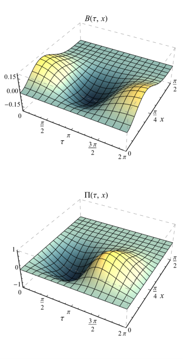 |
 |
Looking at derived solutions we have found a notable change of their profiles when moving along the branch of time-periodic family (with fixed ). While all solutions with amplitudes55 5 By we denote the smallest in absolute value critical points of the mass, , and . are dominated by the harmonic oscillation with profile of bifurcating mode, those beyond the mass extremum have much reacher structure and are of only slightly larger amplitude. For positive branch of family this is visualized on Fig. 5.31, similar we observe for negative values of and for other families .
 |
 |
 |
 |
 |
 |
Having numerically derived time-periodic solutions we have put them into evolution code, as initial conditions, configuration read off from (5.237) and (5.238) at , and monitor their periodicity. On Fig. 5.32 we show the results of such test performed for a time-periodic solution bifurcating from fundamental mode with amplitude which was constructed on a numerical grid with points. Fixing the order of time-integration algorithm (the stage Gauss-RK method of order ) we varied the magnitude of integration step size (to control the error of the time integration). Since the initial conditions contain some amount of error and the time-integration itself gives only an approximate result and we do not observe any signs of instability—still this may happen on a much larger scales. The projections of a phase space, spanned by and , show Lissajous curves. These can be monitored whether they close or not over one or more revolutions. Decreasing an error in the time-integration (by decreasing time step size) we observe a solution to get closer to the periodic orbit. Even for relatively large step sizes, when the time-integration introduces significant amount of numerical noise, the distance to the periodic orbit stays bounded over considered time intervals. The same is observed on a total mass conservation plot. But due to large rounding errors we were not able to decrease the absolute error in total energy below by refining the time-integration method.66 6 A possible source of such error sits in a way of computing the total energy (5.234)-(5.236).

In order to investigate the issue of stability of constructed time-periodic solutions we have considered the Cauchy problem with initial conditions corresponding to perturbed time-periodic solution, with perturbation in initial momenta given by
| (5.260) |
with . We have chosen two representatives of the fundamental family , namely those shown on Fig. 5.31 (with very similar behaviour for the negative branch). For perturbed solution with the evolution is qualitatively the same as we have seen in preceding sections. For relatively small amplitudes of initial perturbation solution stays within a bounded distance from a periodic orbit. This is illustrated for the and case on a series of parametric plots showing time evolution of eigenbasis Fourier coefficients (5.223). While unperturbed trajectories (blue lines) stay periodic (up to numerical errors which are under control—used numerical procedures are consistent), the perturbed solution (gray lines) does not exhibit any recurrences and stays in a bounded and finite distance (over simulated times).
Remarkably this picture does not change as dramatically for solutions with as it does for the EKG system, i.e. no instant or delayed collapse of solutions is observed. On Fig. 5.34 we plot the time evolution of for time-periodic solution () perturbed with Gaussian profiles of increasing amplitudes and . While for perturbations of larger amplitudes () the focusing effect of gravity is strong enough to focus the energy on sufficiently small scales and trigger black hole formation in much shorten times than those shown on Fig. 5.34. (In fact since we are unable to perform evolution up to the black hole formation we identify this process by noting continuous growth of the Kretschmann scalar at the origin, by monitoring .) For considered amplitudes the evolutions stays smooth. An observed modest growth of a Kretschmann scalar for in each of the runs, and connected with that the increase of the mass conservation error, suggests an onset of instability, of the unknown origin (whether this is a numerical artifact, which we have not excluded at the time of writing, or just a long time modulation being a real effect).77 7 One possible explanation would be that, regardless of the size of the controlled perturbation, already the initial data corresponding to the time-periodic solution contains enough and significant error to trigger such growth. In fact the solution was hardly derived using ’only’ grid points, which noticeably is to small to accurately resolve its rough profile. Clearly, we observe different behaviour than for unstable solutions of the EKG system. Therefore, if these solutions are unstable then their unstable modes have small Lyapunov exponents.
5.4 Spherical cavity model
In this section we present and analyze procedures used to construct time-periodic solutions of the system (3.58)-(3.58). The numerical procedure (Section 5.4.2) is an adaptation of Chebyshev pseudospectral spatial discretization, the perturbative construction (Section 5.4.1) shows a different structure of the solutions (compared to AdS case). The analysis of results, presented in Section 5.4.3, is restricted to the small amplitude regime only and concentrates on verification and comparison of these two approaches.
5.4.1 Perturbative construction
We start the perturbative construction of time-periodic solutions to the system (3.59)-(3.62) by taking the following ansatz
| (5.261) | ||||
| (5.262) | ||||
| (5.263) |
together with a time coordinate rescaling , and the perturbative -expansion of the frequency
| (5.264) |
We use the freedom we have in defining the perturbative parameter and set it to the value of the second spatial derivative of a scalar field at the origin at time
| (5.265) |
This choice is dictated by the ease of comparing the perturbative results with the spectral code and its implementation used in numerical construction. As is discussed in Section 4.1.1, in the spectral code we use the field instead of itself and since vanishes at the origin (being the spatial derivative of an even function) the natural choice is to control the second derivative of . In this way, fixing and specifying a real number we choose a single solution of the one-parameter family of time-periodic solutions bifurcating from the frequency . The phase of solutions is fixed by the requirement (as in previously considered models).
At the lowest (linear) order has to be a solution to the homogeneous wave equation (with defined in (3.70))
| (5.266) |
The second order solution (the back-reaction on the metric) can be easily written as the integrals
| (5.267) | ||||
At the third order one gets the inhomogeneous wave equation
| (5.268) |
Due to the incompatibility of eigenbasis functions (3.71) with the regularity conditions, for both reflecting boundary conditions (3.67) and (3.68), the source function in (5.268) cannot be written as a finite combination of the eigenfunctions. This makes the calculations much more involved and these have to be done case by case for each (half-full automatization is still possible). For that case we carry out only the necessary calculations up to the third order to to demonstrate main idea. Despite the fact that the perturbative equations (5.266)-(5.268) are independent of a particular choice of the boundary condition, the construction procedure is very different in each case, for that reason it is considered separately.
Dirichlet boundary condition
A posteriori, we know that for this choice of boundary conditions the calculation are dependent; in the presentation we further restrict ourselves to the case. At the end of this paragraph we comment on generalization to .
As for the solution to the linear wave equation (5.266) we take the single eigenmode (3.71) ()11 1 Note the use of the sinc function .
| (5.269) |
whose amplitude was set such that holds. Then, it is easy to get the back-reaction (the second order solution) by integrating (5.267). At the third order, equation (5.268) has the following separable form
| (5.270) |
Using the orthogonality of cosine basis and setting
| (5.271) |
we reduce this PDE to a system of two independent second order ODEs for and . These have to be solved with the Dirichlet boundary condition at and regularity requirement at (5.265). The condition to meet the proper boundary behaviour for the first of these ODEs fixes the second order frequency correction parameter
| (5.272) |
where is the Euler-Mascheroni constant [148], , are the cosine [147] and sine [151] integral functions respectively, together with one of the integration constants. The boundary condition for cannot be satisfied since only one of the integration constants is fixed by imposing the Dirichlet condition at , while the regularity condition at is violated, even if the second constant is still unspecified. This is a direct consequence of the presence of the resonance to the eigenmode , i.e. the projection does not vanish. This is in contrast to the AdS case, where such cancellations are present. To overcome this difficulty we modify the ansatz for the first order solution (5.269), and instead of just single mode we take, in advance, an infinite combination of all of the eigenmodes whose frequencies satisfy the condition
| (5.273) |
explicitly
| (5.274) |
(we still assume that at the lowest order the frequency is ). Note that ’s fulfilling (5.273) is the subset of (cf. (2.11)). In this way we introduce additional parameters, the eigenmode amplitudes , into our procedure. These will be used, together with , to remove all appearing resonances (or equivalently, to satisfy regularity and boundary conditions) present at the third order. By including subsequent eigenmodes in (5.274) we generate more resonances at the third order, so in fact the number of terms in (5.274) needs to be infinite. Such modification of the first order solution will lead to the inhomogeneous PDE with the source term composed of an infinite number of Fourier modes (an analogous of (5.270))
| (5.275) |
Then, the absence of resonances enforces an infinite system of algebraic equations
| (5.276) |
for and , with an additional normalization condition (5.265)
| (5.277) |
In practice, since we do not have tools (as for the AdS case in even space dimensions) to produce and manipulate effectively the higher order equations, and in particular to determine the conditions (5.276), we truncate the sum in (5.274) at some . To demonstrate that this is the proper way to solve this problem we show the steps for . Approximating by taking
| (5.278) |
we find the , and compute the source in the wave equation (5.268). Then we solve the algebraic equations
| (5.279) | ||||
(which are linear in and cubic in ) and get a nontrivial, real and unique solution
| (5.280) |
(which is given by a lengthy formula in terms of function, so we do not present it here). In addition to the and eigenmode resonances (which are removed by imposing the condition (5.279)) there are higher source projections which cannot be set to zero, since we do not have a sufficient number of free parameters as was mentioned earlier. But, as was seen already, the coefficients in (5.278) are rapidly decreasing with their mode index, so truncating the series (5.274) with moderate number of terms would produce partial but sufficient approximation to a time-periodic solution see Fig. 5.35 (accurate up to the order term with an approximate and back-reaction and ). To sum up, taking more terms in the initial sum (5.274), one gets successively better approximation to the first order solution which is determined by the lack of resonances at third order, at the same time removes more and more resonances (among infinite number of them) present in .
Therefore, cancellation of all of the resonances is possible only if is a very special linear combination of an infinite number of the eigenmodes,22 2 This is also the case for the cubic NLW on a circle [101, 143]. among which the mode has the highest absolute value of the amplitude relative to amplitudes of the other eigenmodes and the frequency of time-periodic solution is . For a general the ansatz for the lowest order solution generalizing (5.274) would be
| (5.281) |
with parameters determined at the third order in a similar way as for the fundamental mode .
Neumann boundary condition
For the Neumann boundary condition, the dispersive case (3.74), there is only one resonance present at each odd perturbative order . This is due to the fact that , i.e. the equation
| (5.282) |
for eigenfrequencies (3.74) has only trivial solution and for any .33 3 This is easy to show by the contradiction. If we assume that (5.282) holds then from the definition (3.74) we get . This condition can be reduced, using a trigonometric identity for , to an algebraic equation whose root for is an algebraic number. This contradicts the assumption that is a transcendental number. Therefore this single resonance can be removed be setting the value of a free parameter . All of the integration constants are fixed by the boundary condition and the normalization condition (5.265). Moreover, since the form of the basis functions (3.71) is independent on , the construction can be performed without specifying .
For time-periodic solution with frequency bifurcating from as first order approximation we take an analogous of (5.269)
| (5.283) |
(with given in Tab. 3.1) and calculate the integrals (5.267). Next, since the wave equation at order (5.268), has exactly the same structure as for the resonant case, i.e. (5.270), we follow the same steps as in the previous paragraph. Both of the solutions and , will contain two integration constants. An additional parameter will be the frequency correction . These constants we fix in a following way. The regularity conditions at the origin and the Neumann condition at the cavity will uniquely determine the function . Imposing the same conditions on the function will fix one integration constant and the parameter
| (5.284) |
(see Tab. 5.5 for numerical values of ). The remaining integration constant (multiplying the term) is a free parameter related to the freedom to define the expansion parameter , which we fix by imposing the condition . In this way we obtain the accurate approximation to the time-periodic solution with being the only parameter, in the nonresonant case, see Fig. 5.36. It is straightforward to continue this construction with the higher order approximation in , with the only (but very serious) limitation that the computations are much more involved and the resulting lengthy formulas one gets are fairly complicated (at least as generated and simplified by the Mathematica). The analysis and manipulation of these is cumbersome (they are not as easy to analyze as in the AdSd+1 case with even), which makes it hard to give some general statements about the obtained time-periodic solutions. For this reason we stop this procedure at order and limit the analysis to the comparison with numerically constructed solutions.
| 0 | 1 | 2 | 3 | ||
|---|---|---|---|---|---|
5.4.2 Numerical construction
We construct the time-periodic solutions of the system (3.59)-(3.62) as follows. We expand both functions and in Fourier series in time and use the following truncated approximation
| (5.285) | ||||
| (5.286) |
where we use the rescaled time coordinate , with the frequency of the solution we are looking for. Instead of expanding the Fourier coefficients , in Chebyshev basis (we do not expand them in the eigenbasis of the linear problem (3.70) since these eigenfunctions do not have correct boundary expansion, see Section 3.3.3, which would cause inefficient polynomial decay of the expansion coefficients in that case) we use the nodal representation, i.e. we operate on the function values on the grid points and as described in Section 4.1.1 and Section 5.1.2.
With radial Chebyshev collocation points (B.13) in space, and collocation points in time , , at each instant of time we calculate values of the fields and at grid points and use them as an input in our time evolution procedure, getting as the output their time derivatives. Equating those to the time derivatives of (5.285) and (5.286) (remembering that ) at the set of Cartesian product grid points , together with the additional equation
| (5.287) |
setting the center value of the dominant mode in the initial data to , we get a nonlinear system of equations for unknowns: , and . This system is solved with the Newton-Raphson algorithm yielding the time-periodic solution of the system (3.59)-(3.61) (the corresponding geometry of space-time given by metric functions and can be determined, at each instant of time, by solving the constraint equations (3.60) and (3.61) for the time-periodic data (5.285) and (5.286) at each constant time slice).
As a starting point for the numerical root-finding algorithm we choose the single eigenmode approximation, fulfilling the condition (5.287), i.e. we set
| (5.288) | ||||
| (5.289) | ||||
| (5.290) |
while looking for solution bifurcating from eigenmode . Such initial conditions, provide a good enough approximation so that the Newton algorithm converges relatively fast even for moderate values of amplitudes .
We use exactly the same methods (with the same solution representation and initial conditions) for both boundary conditions, Dirichlet and Neumann, with only minor modification within the code, in the part calculating the RHS of the wave equation (3.59) (in this case the time derivatives of (5.285) and (5.286)) as is described in Section 4.1.1.
5.4.3 Results
| 0 | 1 | 2 | fit | |
|---|---|---|---|---|
We restrict the presentation of results to a comparison of our perturbative construction with the numerical approach for small amplitude solutions only. Further studies should be devoted to large amplitude solutions and their stability properties (as for in AdS).
To verify results of our methods we look at the profile of the scalar field at (in fact we can make the comparison for any instant of time, but taking is natural, since at that moment all eigenmodes have equal phase since and this is also computationally straightforward). Instead of performing comparison in the physical space, it is convenient to do this in a Fourier space. Therefore we read off the initial data for the field resulting from (5.285). Then we project this function onto the modes (the necessary integrals were computed numerically using the Gauss-Legendre quadrature, see the Appendix A.3), and using the relation (3.75) we get the decomposition of initial data for the function. Repeating this procedure for the time-periodic solutions with different values of the parameter (5.287), we can perform a fit to the numerical data to get the coefficients of polynomial dependence of the expansion coefficients on the amplitude .
For the Dirichlet boundary condition and the fundamental solution () the results are summarized in the Tab. 5.6. These results are in excellent agreement, bearing in mind that for the first order solution (5.274) we have taken only first few terms (up to ). Moreover, from the numerical data we get that the coefficients , scale (in the leading order) as , while the remaining modes behave as , , see Fig. 5.37. This supports our assumption about the form of the solution (5.274)). From this comparison it is evident that including more terms in (5.274) will lead to the successive decrease of coefficient and its convergence to the true value, while will have smaller but growing (in absolute value) numerical values with the number of terms in (5.274). This agreement is strengthened when we compare frequencies of the solutions Fig. 5.37. Fitting an even polynomial in to the numerical data we read off the quadratic term coefficient which has to be compared with the frequency correction obtained by solving the algebraic equations (see Tab. 5.6).
These results validate our perturbative procedure for this model, in particular the form of the first order term in the perturbative expansion, given by the infinite sum (5.274), together with the scheme which gives the unique values of the coefficients and the frequency expansion coefficient .
For the Neumann case, we can perform similar comparison as for the Dirichlet boundary condition. However, having an exact form of and a third order solution determined, we can perform more detailed comparison of perturbative and numerical results (we limit the presentation to the case). First of all, we get the following scaling of the Fourier coefficients and , for (see Fig. 5.38). That is, the first order term (5.261) consist of only one eigenmode, the one with index , while is a linear combination of all eigenmodes. Secondly, we get good agreement of the numerical values of the Fourier coefficients which are shown in Tab. 5.7. For perturbative solution the projections are exact numbers, while for the numerical solution we have performed the least square fitting procedure. Additionally, fitting a polynomial function to the numerical data we get
| (5.291) |
which agrees with an exact perturbative frequency correction (5.284) listed in Tab. 5.5 (the absolute value of relative error is ). The same quality of agreement we obtain when we analyze results for excited solutions .
5.5 Yang-Mills on Einstein Universe
In this section we continue studies of the YM system, initiated in Section 4.2. After discussing perturbative construction of time-periodic solutions (Section 5.5.1) we review the numerical method (Section 5.5.2). Since the perturbative analysis, in contrary to numerical procedure, differs when we consider perturbations around different static solutions (in different topological sectors) both construction and results analysis is considered separately. In Section 5.5.3 we present the results and verify them by comparing numerical and perturbative construction.
5.5.1 Perturbative construction
The perturbative construction of time-periodic solutions is less involved for the YM model when compared to previously analyzed systems, since here we deal with a single PDE. As in previous cases this construction is based on the Poincaré-Lindstedt method, therefore the initial steps we follow here are the same as taken in Section 4.2.2, where the perturbative construction of single mode initial conditions where presented. We introduce new time coordinate through (4.73) and assume series expansion in small parameter () for solution profile and corresponding frequency , as in (4.75) and (4.76) respectively. The Taylor series expansion in of the Eq. (4.74) with (4.75) and (4.76) substituted gives the perturbative second order linear PDEs for . The first four of them are given explicitly in (4.77)-(4.80); the higher order equations contain much more complicated source terms. As in proceeding sections refers to an index of dominant mode in the solution, and since we are looking for bifurcating solutions we assume for the leading order solution
| (5.292) |
(because of used convention here ). We define the perturbative parameter to be the amplitude of the eigenmode at the initial time, i.e. we set
| (5.293) |
which fixes also the phase of time-periodic solution. Then all the higher order equations are solved by assuming decomposition in eigenbasis of as in (4.82), so the time evolution of is governed by (4.83).
Here, when solving the perturbative equations for time-periodic solutions, instead of enforcing (4.84), we relax the initial conditions and for modes other than we set
| (5.294) |
while for
| (5.295) |
Then, free parameters and are used to remove all of the appearing resonant terms and to force the -periodicity of (some of will be used to remove terms with rational frequencies in , which produce spurious secular terms appearing at higher orders). As it turns out, at some orders of the perturbative calculation there may not be enough free parameters available to remove all of the resonances. Then, as for the model of Section 3.2, we modify the solution by adding the homogeneous solution whose amplitude would serve as a missing parameter. Since the construction and the structure of governing equations depends on whether we construct time-periodic solutions around the vacuum static solution or around the kink we discuss these cases separately.
Vacuum sector
The construction of time-periodic solutions in the vacuum topological sector, with , is analogous for the previously considered cases because of the character of the linear spectrum. As before, we need to ensure that at each perturbative order there will be enough parameters availiable to remove all resonances. It turns out that for any the projection in (4.83) vanishes when . The resonant frequencies to present in the source to the wave equation are
| (5.296) |
where is the largest positive integer such that
| (5.297) |
holds, so is the largest resonant frequency present in . From this we get . Thus, at order we will have free integration constants (since one of them is used to satisfy the normalization condition (5.293)). With these and with frequency expansion parameter we can remove at most resonances at order (the resonances at order are removed by using the integration constants left at order and parameters ). However, for there are exactly resonances present at order (at order there is only one resonance which is removed by setting ). Therefore this scheme would break down already at the fourth order where there are two resonances present and we have only one parameter available, namely . Consequently, at each perturbative order me modify the solution to the wave equation by adding the term with the frequency being the -th multiple of , i.e, the term
| (5.298) |
which is itself a solution to the homogeneous equation with in (4.83). Thus, an arbitrary amplitude of (5.298) serve as a remaining parameter to remove all of the resonances appearing at order . Repeating this reasoning with replaced by we see that in this way we get a unique solution, which be constructed up to arbitrary high order.
Kink sector
As we pointed out already the solution to Eq. (4.83) will contain terms which in general are not -periodic functions (especially for frequencies ), with obvious exception for . Therefore we can choose the integration constants appearing at order to eliminate all such terms (for we have parameter which is used to cancel resonant term—the is resonant to itself—then the constant is fixed by the normalization condition). If we have left such terms at order , they would generate secular terms in the solution at order , through spurious resonances (this is the reason why the Poincaré-Lindstedt method failed to give a uniformly bounded solution for a single mode initial data, as was emphasized in Section 4.2.2) and the condition for their absence would fix the parameters . This is equivalent, but the former way of fixing integration constants is the optimal approach. In this way we can proceed to higher order up to appearance of another proper resonance. Even though the eigenfrequencies are irrational numbers (with an exception of the fundamental mode) there is an infinite number of resonances, but they are irregular (as opposed to previous cases, where the eigenfrequencies are equidistant). In fact the resonant set , defined in (2.11), is of measure greater than one for any , since the equation for
| (5.299) |
has infinitely many solutions; for there is only a trivial solution and is a singleton, and this makes the case special. As an example we give below an explicit form of solution to (5.299) for
| (5.300) |
We see that the resonant frequencies are irregularly distributed, hence the construction of time-periodic solutions is not so systematic and has to be carried case by case. Besides that, the strategy of resonance removing is identical to the previous cases. If the resonance to the eigenmode appears at order then we move back to the order and modify the solution by adding to it the term
| (5.301) |
with , whose amplitude will be used at remove this resonance at order . Since then, at any order , there will be two resonances present (up to the appearance of the next resonance for the eigenmode with next index from the set ). These will be removed by utilizing frequency expansion parameter and free integration constant for resonant mode the . In this way the whole procedure can be continued indefinitely with growing number of proper resonances and number of availiable parameters to ensure absence of secular terms.
In general the appearance of a given proper resonance would be hard to predict, nevertheless the order at which the first nontrivial resonance occurs can be precisely predicted. It turns out that before that happens the solution at orders is composed of eigenmodes among which the highest one has index . Whence the first resonance will occur at order since then the resonant mode will be present in , and at the same time would contain Fourier mode (because ). The first resonant eigenmodes and their order of occurrence in perturbative calculation for first few dominant modes are listed in Table. 5.8. It is evident that the first proper resonance appears at relatively high perturbative order, especially for it would be impossible to go to in perturbative construction, in order to check that indeed the terms like (5.301) are necessary. However one cannot neglect the resonances, even if they appear at relatively high perturbative order, since they modify the solution in a significant manner. The two lowest order cases, namely those with and , which are possible to obtain are discussed in the following section when also the properties of constructed solutions are discussed.
Integrals
The products appearing in the perturbative equations are expressed in terms of the following finite sums
| (5.302) |
| (5.303) |
| (5.304) |
| (5.305) |
where the expansion coefficients were derived using the approach given in Appendix D. Those are
| (5.306) |
| (5.307) |
| (5.308) |
where we use the shorthand notation for the normalization constant of eigenfunctions (3.101)
| (5.309) |
The Mathematica assisted guess gives a closed form for the expressions (5.306) and (5.308) in a following form
| (5.310) |
where the nonzero elements are
| (5.311) |
Similarly we get
| (5.312) |
with
| (5.313) |
and denoting the Kronecker delta. The use of (5.310) and (5.312) in place of (5.306) and (5.308) respectively greatly reduces time that Mathematica spends on computation of the expansions and thus allows us to derive a very high order approximation to the time-periodic solutions.
5.5.2 Numerical construction
To find a time-periodic solutions of (3.94) we follow the steps given in Section 2.2.2 of introductory chapter. In this case, where we have a single second order wave equation to solve, the complexity of the overall algorithm greatly simplifies, compared to the case of Einstein’s equations, since the lack of constraints and in addition the number of dynamical variables is reduced here by the factor of two since the velocity and the field are no longer independent (see (4.58) and (4.59)).
As in the previous cases, we use the rescaled time coordinate , with standing for the frequency of time-periodic solution. We assume the following truncated double expansion in the trigonometric series and in the eigenbasis of the linear operator (3.96) of the time-periodic solution
| (5.314) |
(note that this already fixes the phase ). The unknown expansion coefficients are then determined, similarly to the previous cases, by constructing suitable number of algebraic equations. These are taken to be the requirement for the governing equation, namely (3.94), to be identically satisfied at the discrete grid points. Thus, we take a cartesian product grid with collocation points of time coordinate , and collocation points in radial direction , , exactly the same set used in the spatial discretization procedure discussed in Section 4.2.1, suited to the expansion (5.314). Next, at each instant of time we calculate the coefficients
| (5.315) |
and use them as an input in our spectral procedure, which produces as an output their second time derivatives . These values are equated to the second time derivatives calculated directly from (5.314) (taking into account the change of independent variables and the transformation ) again at the set of grid points . We choose the convenient normalization condition as for the time-periodic solutions in AdS, i.e. we control the amplitude of the dominant mode by setting
| (5.316) |
for the solution bifurcating from the eigenmode (of eigenvalue ). This closes the system of nonlinear equations for the expansion coefficients and the frequency of the time-periodic solution which are found by applying the Newton-Raphson algorithm. As in previous models, we initialize this iterative procedure by setting a single mode conditions, i.e, we take
| (5.317) |
5.5.3 Results
Vacuum sector
The time-periodic solutions for case admit a regular structure. For odd and for any the solutions have the following Fourier decomposition
| (5.318) |
| (5.319) |
together with the frequency expansion containing terms with even and odd powers of . Since the time-periodic solution is composed of odd eigenmodes only, the following symmetry holds
| (5.320) |
because of the identity , , for the eigenbasis functions (3.102).
 |
 |
 | |
The structure of solutions with even is different, and these solutions have more symmetries. There are both even and odd eigenmodes present in the solution and the Fourier decomposition of time-periodic solution depends on the parity of ; for even
| (5.321) |
and
| (5.322) |
whereas for odd
| (5.323) |
and
| (5.324) |
The frequency expansion for even contains only even powers of , so . From (5.321)-(5.324) we see that the solution profile exhibits the following symmetries
| (5.325) |
for and .
To visualize results of perturbative construction we plot on Fig. 5.39 density maps of successive terms of the expansion, namely the functions. Clearly, when both the index of dominant mode and the order of perturbative expansion increase the solution oscillates on smaller scales, both in space and time. Note also that the symmetry of solution with respect to the equator of the three sphere, , for is retained at any perturbative order, while for only even order terms (right column) remain symmetric, the odd order terms are antisymmetric (left column).
The change of energy and frequency of time-periodic solutions with the amplitude of dominant mode is presented on Fig. 5.40. The nonlinearity causes the decrease of frequency (the period of oscillation increases) and increase of energy (with ). Though continuous, this dependence on amplitude is not monotonic—for any there exist different solutions having the same period and energy.
We derived numerically solutions on a mesh of points, which produces accurate results for small values of , but gives only rough approximation to true solutions for larger amplitudes. The Newton procedure used to find the time-periodic solutions converges rapidly for small and moderate values of . For larger values its convergence is degraded, while for still larger values the algorithm ceases to converge even when we provide better initial conditions than a single mode approximation (5.317), e.g. by using extrapolation from solutions with smaller values of for which the algorithm converged. The borderline of existence of time-periodic solutions, the limiting values of are computationally difficult to determine. The high amplitude time-periodic solutions have spectra which fall off exponentially but with very small slope, hence to accurately approximate a solution we would need very large number of eigenmodes present in truncated series approximation (5.314). Even using finer grids and taking better initial guess for the Newton root-finding algorithm it would not be possible to greatly extend the bifurcating curves shown on Fig. 5.40.11 1 As we have seen earlier, when discussing time-periodic solutions of other systems, this may be related with the bad definition of parametrization variable. Since the dominant mode amplitude may be bounded there still may exist time-periodic solutions of greater amplitude, e.g. defined by . We left this issue for further studies, and continue discussion using the parametrization (5.293).
However, for any there seems to be a finite range of for which time-periodic solutions exist. Constructing solutions for a few lowest dominant modes we observe that the length of this interval slowly decreases with increasing (separately for even and odd). Using the Padé resummation, as in previous Sections, we were unable to find a reasonable approximation to the limiting values of . In this case the structure of poles of either with or rapidly changes when we change order parameters and . Different also is the character of a frequency bifurcation curve.
Nevertheless, the resumation greatly improves the convergence of perturbative series. The result showing the comparison of numerical data (points) with perturbative expansion of and its resumation is shown on Fig. 5.41 (the case). The off-diagonal Padé approximation, chosen as the best qualitative approximation, greately extends the range of applicability of perturbative result (especially for ). This shows also the agreement of the results of two independent methods used to construct time-periodic solutions (for relatively small the difference of these two methods is dominated by the numerical precision).
Since for small values of the expansion parameter the solutions do not significantly differ from the single mode approximation (as the name suggests the dominant mode is a main component of the solution) we present the results for relatively large values of to make the nonlinear effect clearly visible. On Figs. 5.42 and 5.43 we present the results of numerical calculations for and respectively. For odd the solutions for positive and negative values of are distinct, which is clearly visible on Fig. 5.42, where we present the fundamental solutions. The initial profiles of time-periodic solutions preserve the number of zeros of dominant modes, even when other modes have significant amplitudes (especially for large values of ). This is no longer true for other times, during the evolution the number of zeros changes, in contrast to the linear solutions. This characteristic change of shape in time of function profile, visible also on Fig. 5.43, alongside with frequency change, is the nonlinear effect. It is worth to mention that symmetries, given in Eqs. (5.320) and (5.325), which are apparent on Figs. 5.42 and 5.43, are not forced in numerical code, for given and initial guess for Newton’s algorithm, the parity is preserved through successive iterations.
Kink sector
Up to the occurrence of the first proper resonance, i.e. for , the time-periodic solutions have the following structure. For even the solution is composed of even eigenmodes only
| (5.326) |
| (5.327) |
so it exhibits the following symmetry
| (5.328) |
The frequency contains both even and odd powers of in its Taylor expansion. For odd the eigenmode decomposition depends on parity of , i.e. there is for even
| (5.329) |
| (5.330) |
while for odd
| (5.331) |
| (5.332) |
and the frequency expansion contains only even powers of .
Since by adding the term (5.301) we modify the solution at order these decomposition formulae hold only for (but in practice the order at which first proper resonance appears is very large). Then the eigenmode decomposition at higher perturbative orders greately depends on , since the resonant frequencies do not seem to have any regular structure (cf. 5.300). (The exception is the , which is the fully nonresonant (contrary to fully resonant) case and the formulae (5.329)-(5.332) holds for arbitrary high order .) However, the resonances for do not affect the symmetry of the solution, so the following holds
| (5.333) |
for and , in analogy to (5.325).
As was mentioned already, there are two things which distinguish the time-periodic solutions in the kink and vacuum topological sectors. The first characteristic concerns the frequency of time-periodic solutions. For the family of solutions bifurcating from fundamental mode () the frequency does not depend on . In other words, all time-periodic solutions which as a dominant mode have the eigenmode oscillate with the same frequency even if they are far from the linear regime. This independence on amplitude is shown on Fig. 5.44, where we show results from numerical calculations, this is also confirmed by high order perturbative expansion.
The frequency of solutions based on higher modes depends on amplitude. As for the vacuum topological sector this is not a monotonic function, which is illustrated on Fig. 5.44. But most importantly, the numerical procedure is able to find the solutions with frequencies both smaller and larger than the corresponding frequency of bifurcation point. Also the range of existence is increasing with the index of dominant mode, in contrast to the vacuum case, demonstrated on Fig. 5.40, where the range of existence shrinks with increasing . This makes the kink topological sector different from the vacuum case.
Profiles of solutions for and are shown on Figs. 5.45 and 5.46 respectively. Again, note that the symmetries (5.328) and (5.333) are respected by the numerical code.
Another feature which distinguishes these two topological sectors is the resonant structure. To deal with the proper resonances appearing in perturbative construction we modify the solution by adding some extra terms, which are homogeneous solutions to the governing equations, with amplitude which subsequently serves as a parameter to cancel otherwise occurring secular terms. This was emphasized over current chapter. While for these resonances have regular structure, in the kink topological sector resonances are irregular. Additionally they appear at relatively high perturbative orders. Therefore it is interesting to validate perturbatively constructed solutions with numerical calculations.
The two lowest order and tractable cases are the and , see Tab. 5.8. For the resonance for the eigenmode appears at order and we claim that inclusion of the term (5.301) at order removes the resonance, for the resonance appears at order and the solution modification is done at order . Solving higher order perturbative equations we supported this procedure, since the first proper resonance can be successfully removed and the construction can be continued further. These additional parameters are, for
| (5.334) |
and for
| (5.335) |
Further analysis of perturbative series and comparison with numerically obtained solutions validates our approach. In order to perform quantitative comparison of both approaches it is convenient to rearrange the perturbative series given in Eqs. (4.75) and (4.82) as
| (5.336) |
with the eigenmode expansion coefficients being dependent. Computing numerical solutions for few values of we can determine the dependence on by fitting polynomial in to the numerical data. In particular we can check a leading order scaling with of decomposition coefficients at some instant of time, for convenience we take . These results, with the resonant modes marked, are presented on Fig. 5.47. This is in agreement with perturbative series given in Eq. (5.326) up to .
Moreover the analysis can be even more detailed. Performing the polynomial fit to the resonant mode coefficient (in case) we can compare this with the perturbative calculation. The straightforward approach would fail because of limited numerical precision. This is because for small amplitudes of dominant mode the amplitudes od resonant modes are hidden below the level set by double-floating point precision (which is of order ). In order to be above this threshold we need to take and for and respectively. This if far beyond the linear regime, where the nonlinearities are expected to dominate, and the perturbative approximation does not work. The resolution to this remedy is to use the extended precision arithmetic excellent facilities of Mathematica. Setting the arithmetic precision to significant digits we were able to determine solutions for very small (with residuals not exceeding in absolute value). The results of the fitting procedure and the coefficients extracted from perturbative series are compared in Tab. 5.10. The agreement for lower order coefficients of a polynomial fit is astonishing, while the higher modes are moderately accurate. This would converge both with increasing the number of eigenmodes taken in truncated series expansion (5.314) and with denser probing in (especially for relatively small amplitudes where the perturbative series converge). The same quality of the result we obtain in the case by performing the same analysis, see Tab. 5.10.
5.6 Conclusions
In this chapter we presented the perturbative and numerical methods used to find time-periodic solutions to specific mixed elliptic-hyperbolic systems of PDEs on bounded domains especially to the Einstein equations with negative cosmological constant.
The construction follows a general scheme given in Chapter 2 but the structure of considered equations enforces various modifications. This mainly concerns the perturbative construction where certain additional resonant terms may appear when building successive approximation, and their removal is nontrivial (apart from proper choice of basis functions and the efficient solution to the perturbative equations). As a part of the numerical construction of time-periodic solutions, which itself is rather universal, we have described spatial discretization and in particular we demonstrated how to effectively solve the constraint equations. Finally, we have shown that our approach leads to a stable and convergent numerical scheme. For time evolution problems we have demonstrated superior properties (near preservation of constants of motion) of symplectic time-integration algorithms in long-time simulations.
Extending the results of [112], we have shown the steps of perturbative construction of time-periodic solutions to the EKG system in any space dimension , especially for the physically most interesting case . While for odd the construction procedure (general approach) is challenging (it requires manipulation of long formulae of a very complex structure) it can be greatly simplified in even by using the eigenbasis expansion (algorithmic approach). For even we can reduce the problem of solving coupled PDEs to algebraic equations and a system of second order ODEs. Thus the equations are much easier to solve and the whole procedure is much more efficient.
We presented a way to express the products of eigenfunctions in terms of their (finite in even ) linear combinations, which proved to be a necessary element of the efficient algorithm. In both odd and even cases we give an argument by counting the number of appearing resonant terms, that at each perturbative order we are able to cancel all of the resonances and that produced expressions give a unique solution up to the definition of the expansion parameter. The difference between even and odd also manifests in the numerical construction. For studies of even dimensional cases we have used improved numerical scheme of [112, 114] based on the eigenbasis expansion. For odd dimensional cases, where the former code cannot be used, we employed Chebyshev pseudospectral spatial discretization, which additionally is universal in terms of the space dimension .
Using two independent approaches to the construction of time-periodic solutions we verified our results directly comparing the perturbative and numerical data, performing convergence tests, and finally by the time evolution of the time-periodic solutions (supporting their periodicity). We stressed the importance of appropriate choice of the continuous parameter identifying solutions of a given family (solutions bifurcating from given linear mode). While this choice is not particularly important in the case of small amplitude solutions, the use of proper parametrization is crucial in studies of large amplitude solutions (we noted this in all of the considered problems). Using a center value of the scalar field as an expansion parameter we found that there are no solutions with arbitrarily large mass—the mass function attains its maximum for large amplitude time-periodic solutions. The critical amplitude separates stable branch and unstable branch of solutions. Time evolution of perturbed configurations on the stable branch gives evidence on their nonlinear stability (solutions stays all the time in finite distance to the periodic orbit). In contrast, solutions on the unstable branch unstable branch when perturbed collapse to a black hole almost immediately.
These techniques were applied also to a complex scalar field in the studies of standing waves (counterparts of time-periodic solutions). Simple form of standing wave solutions (static metric and purely harmonic oscillation of matter field) allowed us to study their linear stability problem. In particular, using analytical techniques we were able to solve the eigenvalue problem, proving their linear stability. Using numerical methods we verified our analytical results, in particular consistency of the ansatz we used in the perturbation analysis. Moreover, we determined explicit perturbative (in size of the standing wave solution) expression for the frequency of the oscillatory modes. This linear spectrum turned out, not surprisingly, to be dispersive which explains the nonlinear evolution of perturbed standing waves. These behave in a similar fashion to perturbed (stable) time-periodic solutions and scalar perturbations in spherical perfectly reflecting cavity model with the Neumann boundary condition.
Next we examined, by means of the same methods, time-periodic solutions for vacuum Einstein’s equations using the cohomogenity-two biaxial Bianchi IX ansatz. Explicit exponential nonlinearity of the field equations, in terms of the squashing field makes the perturbative construction rather involved. The perturbative expansion contains both odd and even terms and all of the equations need to be solved at each perturbative order. Among that one additional resonance—unremovable by the straightforward approach—appears at the fifth perturbative order. This induces a modification of lower order solution by inclusion of a homogeneous term. After demonstrating the convergence of the numerical method and the conformity of numerical and perturbative results, we studied the stability problem of time-periodic solutions (here also the mass of the solutions is bounded from above). We confirmed the stability of small amplitude time-periodic solutions. However, large amplitude solutions, exhibits more complex structure than less massive solutions, also behave differently than their scalar ’counterparts’. They do not collapse rapidly when perturbed slightly, and the Kretschmann scalar monitored at the origin does not give any evidence for the instability during long time evolution, but due to numerical difficulties, stability of such configurations remains an open problem requiring further investigation.
In a similar manner we analyzed two remaining models, the perfectly reflecting spherical cavity model and the YM system, aimed mainly to exploit various structures of small amplitude time-periodic solutions. (The issue of reparametrization and detailed stability analysis of constructed solutions are left for further studies.) The linearized spectra of these models can have different character—this affects the form of the solutions (again, this concerns the perturbative expansion, the numerical approach stays unaltered). The analytical construction relies heavily on the fact that resonances appear and their successive removal fixes free parameters (either those in homogeneous terms or the ones appearing as integration constants) in successive perturbative orders. One may naively think that for dispersive linear spectrum resonances are absent and therefore no time-periodic solutions exist then—we show that this is not the case.
For the YM equation the resonant structure require homogeneous terms to be included in solution at more than only one perturbative order (for the kink topological sector with irregular structure of the resonant set) or even at each perturbative order (for the vacuum topological sector with regular structure of the resonant set) during the construction. Without such modifications the number of available parameters will be insufficient to remove all of the appearing resonances and so the procedure will break. (We have used this modification already for time-periodic solutions of the vacuum Einstein equations.) A notable exception is a family of solutions bifurcating from the fundamental mode in the kink topological sector (in this case the bifurcation frequency is an integer, while higher mode frequencies are irrational numbers). For that case the resonant set is a singleton and so there is only one resonance present at each perturbative order. Surprisingly, the oscillation frequency for this family of time-periodic solutions does not depend on the amplitude. This is due to the fact that the structure of perturbative equations, in that particular case, enforces the frequency corrections to vanish. This special case and the presence, in other families of time-periodic solutions, of homogeneous terms (especially their amplitudes) are confirmed, with great accuracy, in the numerically constructed solutions with extended precision arithmetics (in some cases it was necessary to use higher than machine precision in order to verify perturbative prediction).
In all of the above systems the first order approximation to the time-periodic solution is a single eigenmode only. This is also the case for the cavity model with Neumann boundary condition. However, with Dirichlet boundary condition there are more resonances present already at the third (first nontrivial) perturbative order and a single free parameter (the frequency correction) does not suffice to construct a bounded solution with just one mode at the linear level. For that reason the first order solution has to be very specific superposition of eigenmodes such that all of the resonances are absent. We verified this by truncating this infinite series and comparing results (in principle convergence with the truncation order) with the numerics.
To summarize, in this chapter we have presented details of construction of time-periodic solutions to nonlinear systems of PDEs, in particular to the Einstein equations with negative cosmological constant (in the dimensional settings). For each of the considered models we used two independent methods which give consistent results which demonstrated their correctness and give credence to the existence of time-periodic solutions. Additionally, we analyzed constructed solutions and described their properties (including in few cases the stability analysis). These lead us to the conclusion that the existence of time-periodic solutions11 1 Proved by explicit construction. to the nonlinear nondissipative evolution equations on bounded domains seems to be a rule rather than exception. In such class of PDEs systems the time-periodic solutions are dynamical counterparts of the static solutions, thus their derivation (we demonstrated that this is not very difficult) should be the first step in studies of nonlinear wave equations on bounded domains.
In considered models the time-periodic solutions bifurcating from linear modes can be found by means of general methods, both numerical and perturbative. Proposed techniques proved to be extremely efficient; spectral methods in numerical calculations give accurate results with moderate effort,22 2 When the spectral convergence rate is observed. the perturbative expansion procedure (preferably with use of eigenbasis functions of associated linear operator), assisted with CAS, produces high order approximation. In addition, we have shown how to discretize equations with the spectral decomposition, and in particular how to solve the constraint equations effectively. The numerical code was used not only to find time-periodic solutions but was also central part of the time-evolution code. Presented methods with use of symplectic integrators lead to stable near energy preserving numerical scheme allowing for long time evolutions.
Chapter 6 Summary and Outlook
In this closing chapter we provide summary of the thesis and give several remarks on future work in the field.
6.1 Summary
In this thesis we studied dynamics of nonlinear waves on bounded domains. Because of our primary motivation, (in)stability problem of AdS, we have devoted most space to the analysis of equations describing perturbations of aAdS spaces. We have demonstrated the existence of (strictly) time-periodic solutions within each of analyzed systems thus showing that time-periodic solutions are common to the nondissipative nonlinear PDEs on bounded domains. In particular, we constructed time-periodic solutions to the vacuum Einstein equations with negative cosmological constant under cohomogenity-two biaxial Bianchi IX ansatz. Even though the analyzed systems differ in details, time-periodic solutions can be constructed by means of general procedures: the perturbative Poincaré-Lindstedt method and Newton’s root-finding numerical algorithm based on pseudospectral discretization, as described in Chapter 2.
We made extensive tests and detailed comparisons of our two independent constructions and direct numerical evolution of initial data corresponding to time-periodic solution. All of them corroborate the correctness of our approaches. We analyzed the properties constructed solutions, in particular we demonstrated their stability. For the complex scalar field case of the EKG system we investigated in more detail the linear stability of standing wave solutions. We showed the dispersive character of the spectrum of their linear perturbations from which we also infer the change of stability at the turning point for any family of solutions.
Studying perfectly reflecting spherical cavity model we gave evidence that turbulent dynamics is not an exclusive domain of aAdS spaces but can be also observed in confined geometries with zero (see also [121]). Concerning the question how the character of the linear spectrum affect the nonlinear dynamics, we analyzed by weakly nonlinear perturbative expansion small amplitude initial data and highly nonlinear regime by means of numerical solution of initial or initial-boundary value problems. In all considered cases with dispersive spectra we observed spreading of the initial perturbation which for small amplitude was preventing solution to collapse (for self-gravitating models). Moreover, we observed studying the YM system (in perturbative calculations) that the resonances are equally common in dispersive and nondispersive cases and that in both cases in the long time evolution the energy cascade eventually stops.
Above that we have developed numerical methods intended for long and stable time evolution of Einstein equations with negative cosmological constant and related problems. These methods are based on MOL approach with pseudospectral discretization in space and RK time integration. We verified their robustness and in particular we demonstrated superiority of symplectic ODE integrators.
Although our results are not rigorous (neither we provide proof of existence of time-periodic solutions nor we prove the convergence of derived perturbative series) we hope that the presented evidence leave little doubt.
6.2 Future work
This thesis focuses on only a few particular aspects of a very interesting and broad area lying on the interface of General Relativity and turbulence. There are many further directions to pursue or questions to answer, let alone attempts to prove the existence of time-periodic solutions we have constructed. Below we enumerate some of them:
- i)
Do all time-periodic solutions of the EKG model on the unstable branch collapse to a black hole? (We have confirmed this only for several points on the unstable branch.) Why do we not observe a similar behaviour (large amplitude oscillations) as in the complex scalar field case?
- ii)
The results of stability studies of time-periodic solutions within the cohomogenity-two biaxial Bianchi IX ansatz are not conclusive; it would be particularly valuable to refine these results.
- iii)
What is the long-time dynamics of perturbed unstable standing wave solutions?
- iv)
Concerning the problem of stability of the time-periodic solutions, it would be interesting to see whether these solutions are stable with respect to perturbations outside the ansatz, e.g. by considering generalizations of the YM field to the sphaleron sector [130, 45], or by considering coupled Einstein-Yang-Mills system, or by relaxing the cohomogenity-two biaxial Bianchi IX ansatz to include triaxial case [24].
- v)
Full understanding of the nonlinear evolution of solutions to the YM equation is certainly beyond the reach of our currently developed mathematical technology. Therefore, it would be valuable to study the system (4.97) as a particular low dimensional approximation of the original equation.
- vi)
Recently, there has been considerable interest in studies of the EKG system with a massive scalar field [90, 91]. In the context of AdS instability this seems to be ’the next step’ towards answering the question how the boundary conditions, imposed on the conformal boundary of the AdS space, affect global dynamics. Under particular conditions, for massive scalar field, there is a freedom to consider more general boundary data [23], which require an extensive exploration.
- vii)
Exploring the perfectly reflecting spherical cavity model one can study more systematically the effect of dispersive character of the linear spectrum on nonlinear dynamics either by considering system with angular momentum [122] (which by a centrifugal barrier term introduces the discrete parameter controlling dispersion relation) or by going to higher dimensions (strikingly the case is special in a sense that with Dirichlet boundary condition the linear spectrum is equidistant (nondispersive), which is not the case for both for Dirichlet and Neumann boundary conditions).
- viii)
Since the analysis of the Einstein equations is particularly involved (both analytically and numerically) its seems useful to analyze simpler models. The YM system considered here turned out to not to be the best model of the AdS dynamics (the energy transfer eventually stops, even though the spectrum is nondispersive). Alternative toy model would be semi-linear wave equation derived from the cohomogenity-two biaxial Bianchi IX ansatz by ’ignoring’ the metric functions and (Section 3.2). The resulting PDE for the squashing field has a nondispersive spectrum and the nonlinearity of geometric nature. Preliminary studies have shown the existence of time-periodic solutions and a blow-up phenomena for relatively small initial data.
- ix)
Finally, with methods presented in this thesis one can effectively analyze (in particular perform the time evolution) cases when the turbulence is ’not active’. For field configurations developing steep gradients, for which black hole formation or blow-up is expected, current methods are fairly inefficient. Still more involved techniques like moving mesh methods [38] may be required.
Appendix A Orthogonal polynomials
In this chapter we collect the most important facts about orthogonal polynomials which appear in this thesis. We refer to general resources [1, 125, 119, 139] for more details; in connection with spectral methods we especially recommend references [34, 134].
A.1 The Jacobi polynomials
The Jacobi polynomials of degree , where both parameters , , are defined as regular solutions to the second order differential equation
| (A.1) |
They form an important class of orthogonal polynomials in numerical analysis.
- i)
Weight function
(A.2) - ii)
The orthogonality relation
(A.3) .
- iii)
Customary normalization
(A.4) - iv)
First few polynomials
(A.5a) (A.5b) (A.5c) General formula
(A.6) - v)
- vi)
Derivative
(A.9) - vii)
Relation with hypergeometric functions
(A.10) - viii)
- ix)
A.2 The Chebyshev polynomials
Chebyshev polynomials are orthogonal polynomials with respect to the weight function solving the following differential equation
| (A.15) |
- i)
Orthogonality property
(A.16) - ii)
Trigonometric definition
(A.17) - iii)
First few polynomials
(A.18a) (A.18b) (A.18c) - iv)
Special values of
(A.19) (A.20) (A.21) - v)
Integration of Chebyshev polynomials
(A.22) (A.23) (A.24) (A.25) - vi)
For an even function which has the expansion in terms of even Chebyshev polynomials only
(A.26) a value of at can be computed referring to the expansion coefficients only, from (A.20) we have
(A.27) - vii)
Zeros
(A.28) (known as Chebyshev points of the first kind or Chebyshev Gauss points).
- viii)
Extrema
(A.29) (these are known as Chebyshev points of the second kind or Chebyshev-Gauss-Lobatto points).
- ix)
Relation with Jacobi polynomials
(A.30)
A.3 The Legendre polynomials
Legendre polynomials are regular solutions to the Legendre’s differential equation
| (A.31) |
They are a special case of the Jacobi polynomials with (subclass of the ultraspherical polynomials).
- i)
Orthogonality property
(A.32) - ii)
Rodrigues representation
(A.33) - iii)
First few polynomials
(A.34a) (A.34b) (A.34c) General formula
(A.35) - iv)
Gauss-Legendre quadrature approximates the integral
(A.36) for smooth function , by the finite sum
(A.37) where the weights are
(A.38) and the abscissas (quadrature points) are the zeros of . The error of Gauss-Legendre quadrature is
(A.39) From this it follows that the Gauss-Legendre quadrature is exact for polynomials of order .
Appendix B Polynomial pseudospectral methods in spherical symmetry
In this chapter we point out difficulties of using spectral algorithms with spherical coordinates and give the standard solution using Chebyshev polynomials which avoids singularity at the origin.
B.1 Chebyshev method
The Chebyshev polynomials (see Section A.2) are one of the most used class of orthogonal polynomials in spectral methods. They are not only distinguished by the analytic form of the quadrature nodes and weights but also by their simple form and the connection with the Fourier series makes them particularly important in the context of spectral methods.
We assume that is a smooth function (defined on interval ), which is well approximated in the finite dimensional subspace of that satisfy prescribed boundary conditions. Taking Chebyshev polynomials as basis functions of , any function can be approximated as
| (B.1) |
The expansion coefficients can be effectively computed using the trigonometric relation (A.17) with Fast Fourier Transform (FFT) algorithm, see e.g. [34]. Alternatively these can be computed using either quadrature formulae or by solving the linear algebraic system
| (B.2) |
where and are suitably chosen grid points.
The expansion (B.1) can be written using the Lagrange interpolation polynomial
| (B.3) |
which is mathematically equivalent to (B.1) when the grid points are chosen appropriately [88]. This polynomial interpolation representation is particularly convenient while working with (anti)symmetric functions (as is the case in spherical symmetry, see discussion in the following section). For any choice of nodes the Lagrange interpolating polynomials are
| (B.4) |
with the property
| (B.5) |
The formulae (B.3) and (B.4) (referred to as the Lagrange form) are usually mentioned in numerical analysis literature, but (B.4) is neither computationally efficient nor numerically stable [17]. Therefore, following [17] we prefer the more optimal form of interpolating polynomial. Introducing weights
| (B.6) |
we rearrange (B.3) and (B.4) to the following symmetric form
| (B.7) |
which is referred as barycentric formula.
The weights (B.6) can be calculated analytically on few sets of grid points. Specifically for Chebyshev points of the second kind (A.29), used in our numerical codes, these are given explicitly
| (B.8) |
(note that these are not unique, but due to the special form of (B.7) the common factor cancels out). We refer to (B.8) as Chebyshev (barycentric) weights.
Further, using the interpolating representation (B.7), derivatives of the interpolant at the grid points can be computed using the differentiation matrices (as in the standard pseudospectral method), so
| (B.9) |
The element -th of -th order differentiation matrix () can be expressed by the following recurrence relation (the hybrid formula)
| (B.10) |
for , where is the identity matrix.
B.2 Spherical symmetry
Each of the problems encountered in this thesis suffer for the singularity of the spherical coordinate system. In most cases we use the basis functions (the eigenbasis associated with the linear operator) for the expansion of approximated functions. These functions are regular at the origin and also convenient to use. But not always they are compatible with the boundary expansion at the outer boundary for the nonlinear problem. Therefore other set of functions should be used and these typically are Chebyshev polynomials [34].
The difficulty in using polynomial spectral methods in spherical coordinate systems is twofold. First, the equations written in spherical coordinate system are typically singular at the origin (especially those containing Laplacian operator). Second, for polynomial interpolation methods the grid points are clustering near the domain boundaries which for the time-dependent problems severely restricts time steps taken (because of stability restrictions). These issues can be easily resolved by noting that the singularity of the Laplace operator written in spherical coordinates is just an apparent singularity. The solution to a differential equation is usually smooth at the origin and it should be taken into account in numerical calculations. Additionally, more grid points in the region where the approximated function is smooth is usually unnecessary.
While many resolutions for the spectral methods in spherical (and related) coordinate systems have been proposed for various problems (see, e.g. [34, Chapter 18]) we prefer to use the ’double covering’ method [141]. We demonstrate this approach by approximating and computing derivatives of smooth function defined on the unit radial interval . To weaken the coordinate singularity at the origin we extend the radial coordinate to (without rescaling) and use the (anti)symmetry (with respect to ) of approximated functions to reduce actual calculations to within . We assume be a smooth function such that
| (B.11) |
holds, with or for even or odd cases respectively. Then we take Chebyshev grid points (A.29)
| (B.12) |
covering the interval and composing the computational grid such that, there are exactly points of the ’physical’ part of the grid (), i.e.
| (B.13) |
(Here we adapt a convention that the quantities defined on a computational grid are denoted by over tilde while these on the ’physical’ part of the grid are not.) In this way we exclude the origin from our scheme, since only asymptotically and there is no clustering at , so we do not need to impose ’pole conditions’ to ensure regularity.
A finite-dimensional polynomial interpolation of is (cf. (B.7))
| (B.14) |
and the -th derivative of the interpolant of at the computational nodes can be computed using the differentiation matrices (B.10). Denoting by and the values of function and its -th derivative at the grid nodes respectively, we have
| (B.15) |
where we explicitly divide the matrix (composed of and the barycentric weights: , , , ) into four blocks. Since we are interested in the values of the derivative at the ’physical’ part of the grid only, i.e. in , , we rewrite (B.15) as
| (B.16) |
where we have used (anti)symmetry of the function . In this way we reduce the number of floating-point operations (thus the computational complexity) by the factor of two when computing the derivatives (the necessary matrices in (B.16) are calculated only once at the initialization phase). To simplify notation we adapt the following convention to the differentiation matrices of (anti)symmetric functions
| (B.17) |
with plus sign for and minus sign for in (B.11).
Whenever the value of the function at which is not a grid node (, for any ) is needed we use the barycentric interpolation formula (B.7). For that we use the computational grid (B.13) with corresponding barycentric weights and the function values for at the grid nodes given by the (anti)symmetry. Then the barycentric formula reads
| (B.18) |
For example, the value of the symmetric function at the origin is
| (B.19) |
since and holds for and from symmetry of we have for .
Note that this approach is equivalent to (A.27) where the coefficients of even Chebyshev polynomials expansion are used. In the computations presented in this thesis we prefer to use the barycentric formulation with the differentiation matrices approach because this is convenient in solving the constraints (elliptic PDEs), moreover for relatively small grids we can reduce the complexity of the algorithm computing derivatives by the factor compared to commonly used FFT based differentiation.
Appendix C Runge-Kutta methods
In this chapter we consider one-step methods for the systems of ODEs. In particular we discuss the Runge-Kutta methods. Here we give only necessary definitions and state key theorems characterizing the methods. We motivate the use of specialized methods for the problems considered in this thesis.
For proofs and more details concerning methods for ODE systems we refer to specialized series of books [83, 84, 82] and references therein to research papers.
C.1 Definition
Definition 1 (The Runge-Kutta methods).
Let , () be real numbers and let be defined by
| (C.1) |
The method
| (C.2) | ||||
is called an s-stage Runge-Kutta method for ODE system
| (C.3) |
with sufficiently well behaved (). When for we have an explicit (ERK) method. If for and at least one , we have an diagonal implicit Runge-Kutta method (DIRK). If in addition all diagonal elements are identical ( for ), we speak of a singly diagonal implicit (SDIRK) method. In all other cases we speak of an implicit Runge-Kutta method (IRK).
The coefficients , and of RK methods are commonly listed in a table (the Butcher tableau)
| (C.4) |
C.2 Explicit methods
The ease of use of explicit methods makes them particularly popular (this does not mean this is always the optimal choice). One of the best known ERK method is the classical fourth order
| (C.6) |
known from its balance between the cost and accuracy. Many higher order methods where constructed over the years of research, but they are necessary much more computationally costly, since the number of stages ( in formulas (C.1) and (C.2)) rapidly increases with (in fact for no ERK method exists of order with stages).
It is often advantageous to continue integration with dynamically changing step size . This is either done by using Richardson extrapolation or by using RK formulae which contain two numerical approximations for where their difference yields an estimate of the local error which is then used for step size control. The embedded ERK methods are characterized by the Butcher tableau
| (C.7) |
such that
| (C.8) |
is of order , and
| (C.9) |
is of order (usually or ).
The ERK method used in this thesis is the Dormand-Prince method with , (known as DOPRI5), which has the following coefficients
| (C.10) |
The characteristic feature of the Dormand-Price methods [60] is that they have a minimal error coefficients of the higher order result ( here) which is then used as numerical solution (as opposed to Fehlberg methods [62] which use the lower order approximation as an initial value for the next step).
The part of the computations in this thesis using (C.10) where obtained by adapting the DOPRI5 routine of the FORTRAN code 11 1 The source codes including also few usage examples are available at the webpage http://goo.gl/oDPoN9. implementing the adaptive step method (C.10).
C.3 Implicit methods
For implicit methods, the in (C.2) are not given explicitly (as is for ERK). The fully implicit method of stages constitute of equations to be solved at each step (for ODE system of size ). This makes the IRK more complicated to implement and simultaneously more expensive to use than the ERK methods. Nevertheless, the properties like larger domains of stability make IRK especially useful for stiff equations, where the possibility to make larger step sizes compensates the cost of solving nonlinear system for ’s. Moreover, the importance of some IRK for Hamiltonian systems, where quality is more important than accuracy, is discussed later.
One of the class of IRK are the collocation methods, and in particular Gauss methods (known also as Gauss-Legendre RK methods), which are collocation methods based on the Gaussian quadrature formulae, i.e. the in (C.20) are the zeros of the shifted Legendre polynomial (see Section A.3) of degree
| (C.11) |
The simplest and probably the best known implicit method is the implicit midpoint rule
| (C.12) |
which is the lowest order Gauss method. The higher order implicit Gauss RK schemes are for orders (the Hammer-Hollingsworth method)
| (C.13) |
and (the Kuntzmann-Butcher method)
| (C.14) |
Schemes of order can be constructed for any (see [39] where also methods of orders and are explicitly given). Their stability domains are precisely the left half-plane (these methods are A-stable). However, our main interest of these methods is due to their properties when applied to the Hamiltonian systems.
Hamiltonian systems is given by
| (C.15) |
(), where the Hamiltonian function is the first integral. Moreover, the flow corresponding to (C.15) is symplectic, it preserves the differential 2-form
| (C.16) |
Special properties of Hamiltonian systems motivated studies of numerical methods suitable for the ODEs of this special form (C.15).
Definition 3.
A one-step method is called symplectic if for every smooth Hamiltonian and for every step size the mapping (the transformation defined by the method)
| (C.17) |
is symplectic, i.e. preserves the differential 2-form (C.16).
An important property of the Gauss methods is stated in the following theorem
Theorem 1 ([83, p. 315, Theorem II.16.5]).
The implicit -stage Gauss methods of order are symplectic for all .
The characteristic feature of all of symplectic RK methods is summarized in the following theorem
Theorem 2 ([83, p. 316, Theorem II.16.6]).
If the matrix with elements , () satisfies , then the Runge-Kutta (C.2) method is symplectic.
An important implication of this theorem is that the ERK methods are never symplectic. Moreover the most familiar classes of IRK (Radau IA and IIA, or Lobatto IIIA, IIIB and IIIC methods) are also not symplectic. Although, the Lobatto IIIA-IIIB pair, composed into partitioned Runge-Kutta method (see below) play important role as it generalizes the Störmer-Verlet scheme [82].
The important property of symplectic methods is preservation of the Hamiltonian and other first integrals.
C.4 Partitioned methods
Let us consider differential equations in the partitioned form ()
| (C.19) |
, (with , not necessarily equal) with special case including (C.15).
Definition 4 (Partitioned Runge-Kutta method).
Let , and , be the coefficient of two Runge-Kutta methods. A partitioned Runge-Kutta method (PRK) for the solution of (C.19) is given by
| (C.20) | ||||
The idea behind (C.20) is to take two RK methods, and to treat the -variables with the first method (with coefficients , ), and the -variables with the second method (coefficients , ). The following theorem gives the condition for symplecticity of (C.20)
Theorem 4 ([83, p. 326, Theorem II.16.10]).
In particular, for separable Hamiltonian systems
| (C.23) |
it is possible to obtain explicit symplectic methods. If the PRK method (C.20) consist of diagonally implicit and explicit methods
| (C.24) | ||||
respectively, then the resulting scheme is explicit. Moreover, assuming and () without loss of generality, then the symplecticity condition (C.22) becomes
| (C.25) | ||||
so that the method (C.20) is characterized by
| (C.26) |
For example, the fourth order method given in [161] has the following set of coefficients, of the first Butcher tableau
| (C.27) | ||||
and of the second one
| (C.28) | ||||
Appendix D Interaction coefficients
In this chapter we briefly review methods we use to calculate integrals (interaction coefficients) appearing in perturbative calculations.
D.1 General formula
In perturbative calculations we need to expand different quantities into a linear combination of eigenfunctions themselves (the interaction coefficients). This requires computation of integrals of products of eigenfunctions. Let assume (for generality) that there is a given set of orthogonal functions on a interval with a weight function
| (D.1) |
( is the Kronecker delta). We want to calculate an integral of the form
| (D.2) |
for , where is some well behaved function. Because the eigenbasis functions which we encounter here are polynomials in we reduce the integrand (D.2) to the sum of the cosine and sine products. Then if this integral is convergent (which we assume is true) we make use of the Euler beta function [146], i.e.
| (D.3) |
which is valid for integer powers . Reducing of each the products in (D.2) to the sum (allowing for use of (D.3)), and changing variables (by rescaling the interval to ) the integral (D.2) can be written as
| (D.4) |
where we use the sum rule, assuming that this integral is convergent whence both and , for any . The dimension of summation multi-index and real coefficients depend on a specific form of the integral (D.2). In exactly the same way we can obtain the value of the integrals .
D.2 Example
Let us consider the YM model (see Section 3.4) to illustrate the above. For this model we have , and the eigenfunctions (3.102) are
| (D.5) |
(we rewrite (3.101) for convenience). In order to use the formula (D.4) we express the eigenfunctions using the series representation of the Jacobi functions (A.6) to get
| (D.6) |
As an example let us calculate the projection . Denoting by the normalization constant in (D.6)
| (D.7) |
we have
| (D.8) |
since for any the powers of and in this integral are always greater than as is required for convergence. This result is a special case of (D.4) with , , and . Then, calculating (D.8) for specific values of indices we have, e.g.
| (D.9) | ||||
| (D.10) | ||||
| (D.11) | ||||
| (D.12) | ||||
| (D.13) |
Therefore in general we have
| (D.14) |
References
- [1] M. Abramowitz and I.A. Stegun “Handbook of Mathematical Functions: With Formulas, Graphs, and Mathematical Tables”, Applied Mathematics Series Dover Publications, 1972 URL: http://books.google.pl/books?id=MtU8uP7XMvoC
- [2] M Alcubierre “Introduction to 3+1 Numerical Relativity” Oxford University Press, 2008
- [3] David˜M. Ambrose and Jon Wilkening “Computation of symmetric, time-periodic solutions of the vortex sheet with surface tension” In P. Natl. Acad. Sci. USA 107.8, 2010, pp. 3361–3366 DOI: 10.1073/pnas.0910830107
- [4] David˜M. Ambrose and Jon Wilkening “Computation of Time-Periodic Solutions of the Benjamin-Ono Equation” In J. Nonlinear Sci. 20.3 Springer-Verlag, 2010, pp. 277–308 DOI: 10.1007/s00332-009-9058-x
- [5] David˜M. Ambrose and Jon Wilkening “Dependence of Time-periodic Vortex Sheets with Surface Tension on Mean Vortex Sheet Strength” In Procedia {IUTAM} 11.0, 2014, pp. 15 –22 DOI: 10.1016/j.piutam.2014.01.044
- [6] E. Anderson et al. “LAPACK Users’ Guide” Philadelphia, PA: Society for IndustrialApplied Mathematics, 1999
- [7] S.˜J. Avis, C.˜J. Isham and D. Storey “Quantum field theory in anti-de Sitter space-time” In Phys. Rev. D 18 American Physical Society, 1978, pp. 3565–3576 DOI: 10.1103/PhysRevD.18.3565
- [8] Jayashree Balakrishna, Edward Seidel and Wai-Mo Suen “Dynamical evolution of boson stars. II. Excited states and self-interacting fields” In Phys. Rev. D 58 American Physical Society, 1998, pp. 104004 DOI: 10.1103/PhysRevD.58.104004
- [9] Venkat Balasubramanian et al. “Holographic Thermalization, Stability of Anti-de Sitter Space, and the Fermi-Pasta-Ulam Paradox” In Phys. Rev. Lett. 113.7, 2014, pp. 071601 DOI: 10.1103/PhysRevLett.113.071601
- [10] D. Bambusi and N.N. Nekhoroshev “A property of exponential stability in nonlinear wave equations near the fundamental linear mode” In Phys. D 122.1–4, 1998, pp. 73 –104 DOI: 10.1016/S0167-2789(98)00169-9
- [11] D. Bambusi and N.N. Nekhoroshev “Long Time Stability in Perturbations of Completely Resonant PDE’s” In Acta Appl. Math. 70.1-3 Kluwer Academic Publishers, 2002, pp. 1–22 DOI: 10.1023/A:1013943111479
- [12] Hans Bantilan, Frans Pretorius and Steven˜S. Gubser “Simulation of asymptotically spacetimes with a generalized harmonic evolution scheme” In Phys. Rev. D 85 American Physical Society, 2012, pp. 084038 DOI: 10.1103/PhysRevD.85.084038
- [13] C.˜A.˜Ball“’on Bayona and N.˜R.˜F. Braga “Anti-de Sitter boundary in Poincaré coordinates” In Gen. Relat. Gravit. 39.9 Springer US, 2007, pp. 1367–1379 DOI: 10.1007/s10714-007-0446-y
- [14] R. Becerril, A. Bernal, F.S. Guzm“’an and U. Nucamendi “Stability properties of Q-stars” In Phys. Lett. B 657.4-5, 2007, pp. 263–268 DOI: 10.1016/j.physletb.2007.07.077
- [15] C.M. Bender and S.A. Orszag “Advanced Mathematical Methods for Scientists and Engineers I: Asymptotic Methods and Perturbation Theory”, Advanced Mathematical Methods for Scientists and Engineers Springer, 1999 URL: http://books.google.pl/books?id=-yQXwhE6iWMC
- [16] G.˜P. Berman and F.˜M. Izrailev “The Fermi-Pasta-Ulam problem: Fifty years of progress” In Chaos 15.1, 2005
- [17] J. Berrut and L. Trefethen “Barycentric Lagrange Interpolation” In SIAM Rev. 46.3, 2004, pp. 501–517 DOI: 10.1137/S0036144502417715
- [18] Massimiliano Berti and Michela Procesi “Nonlinear wave and Schrödinger equations on compact Lie groups and homogeneous spaces” In Duke Math. J. 159.3 Duke University Press, 2011, pp. 479–538 DOI: 10.1215/00127094-1433403
- [19] J Bic“’ak, M Scholtz and P Tod “On asymptotically flat solutions of Einstein’s equations periodic in time: I. Vacuum and electrovacuum solutions” In Classical Quant. Grav. 27.5, 2010, pp. 055007 URL: http://stacks.iop.org/0264-9381/27/i=5/a=055007
- [20] J Bic“’ak, M Scholtz and P Tod “On asymptotically flat solutions of Einstein’s equations periodic in time: II. Spacetimes with scalar-field sources” In Classical Quant. Grav. 27.17, 2010, pp. 175011 URL: http://stacks.iop.org/0264-9381/27/i=17/a=175011
- [21] P. Bizo“’n and Z. Tabor “On blowup of Yang-Mills fields” In Phys. Rev. D 64 American Physical Society, 2001, pp. 121701 DOI: 10.1103/PhysRevD.64.121701
- [22] P. Bizo“’n et al. “Vacuum gravitational collapse in nine dimensions” In Phys. Rev. D 72 American Physical Society, 2005, pp. 121502 DOI: 10.1103/PhysRevD.72.121502
- [23] Piotr Bizo“’n “Is AdS stable?” In Gen. Relat. Gravit. 46.5 Springer US, 2014
- [24] Piotr Bizo“’n, Tadeusz Chmaj and Bernd˜G. Schmidt “Codimension-Two Critical Behavior in Vacuum Gravitational Collapse” In Phys. Rev. Lett. 97 American Physical Society, 2006, pp. 131101 DOI: 10.1103/PhysRevLett.97.131101
- [25] Piotr Bizo“’n, Tadeusz Chmaj and Bernd˜G. Schmidt “Critical Behavior in Vacuum Gravitational Collapse in 4+1 Dimensions” In Phys. Rev. Lett. 95 American Physical Society, 2005, pp. 071102 DOI: 10.1103/PhysRevLett.95.071102
- [26] Piotr Bizo“’n and Joanna Jamu“.zna “Globally Regular Instability of 3-Dimensional Anti-De Sitter Spacetime” In Phys. Rev. Lett. 111 American Physical Society, 2013, pp. 041102 DOI: 10.1103/PhysRevLett.111.041102
- [27] Piotr Bizo“’n and Andrzej Rostworowski “Gravitational turbulent instability of AdS5” URL: http://goo.gl/LZx0g9
- [28] Piotr Bizo“’n and Andrzej Rostworowski “Weakly Turbulent Instability of Anti-de Sitter Spacetime” In Phys. Rev. Lett. 107 American Physical Society, 2011, pp. 031102 DOI: 10.1103/PhysRevLett.107.031102
- [29] Piotr Bizo“’n and Bernd˜G Schmidt “How to bypass Birkhoff through extra dimensions: a simple framework for investigating the gravitational collapse in vacuum” In Int. J. Mod. Phys. D 15.12 World Scientific, 2006, pp. 2217–2222 DOI: 10.1142/S0218271806009649
- [30] Alexander˜I. Bobenko and Sergej˜B. Kuksin “The nonlinear Klein-Gordon equation on an interval as a perturbed Sine-Gordon equation” In Comment. Math. Helv. 70.1 Birkhäuser-Verlag, 1995, pp. 63–112 DOI: 10.1007/BF02566000
- [31] J. Bourgain “Construction of periodic solutions of nonlinear wave equations in higher dimension” In Geom. Funct. Anal. 5.4 Birkhäuser-Verlag, 1995, pp. 629–639 DOI: 10.1007/BF01902055
- [32] J˜P Boyd “A numerical calculation of a weakly non-local solitary wave: the breather” In Nonlinearity 3.1, 1990, pp. 177 URL: http://stacks.iop.org/0951-7715/3/i=1/a=010
- [33] J.˜P. Boyd “A numerical comparison of seven grids for polynomial interpolation on the interval” In Comput. Math. Appl. 38.3–4, 1999, pp. 35–50 DOI: 10.1016/S0898-1221(99)00204-7
- [34] J.˜P. Boyd “Chebyshev and Fourier Spectral Methods: Second Revised Edition”, Dover Books on Mathematics Dover Publications, 2001 URL: http://books.google.pl/books?id=lEWnQWyzLQYC
- [35] Dieter˜R. Brill and James˜B. Hartle “Method of the Self-Consistent Field in General Relativity and its Application to the Gravitational Geon” In Phys. Rev. 135 American Physical Society, 1964, pp. B271–B278 DOI: 10.1103/PhysRev.135.B271
- [36] Alex Buchel, Luis Lehner and Steven˜L. Liebling “Scalar collapse in AdS spacetimes” In Phys. Rev. D 86.12, 2012, pp. 123011 DOI: 10.1103/PhysRevD.86.123011
- [37] Alex Buchel, Steven˜L. Liebling and Luis Lehner “Boson stars in AdS spacetime” In Phys. Rev. D 87.12 American Physical Society, 2013, pp. 123006 DOI: 10.1103/PhysRevD.87.123006
- [38] Chris˜J. Budd, Weizhang Huang and Robert˜D. Russell “Adaptivity with moving grids” In Acta Numer. 18, 2009, pp. 111–241 DOI: 10.1017/S0962492906400015
- [39] J.˜C. Butcher “Implicit Runge-Kutta processes” In Math. Comput. 18.85, 1964, pp. 50–50 DOI: 10.1090/S0025-5718-1964-0159424-9
- [40] Eugenio Calabi and Lawrence Markus “Relativistic space forms” In Ann. Math. 75.1 JSTOR, 1962, pp. 63–76
- [41] Mark Caprio “CustomTicks package” URL: http://goo.gl/e6sJCB
- [42] R“’emi Carles and Erwan Faou “Energy cascades for NLS on the torus” In Discrete Cont. Dyn. B 32 American Institute of Mathematical Sciences, 2012, pp. 2063–2077 DOI: 10.3934/dcds.2012.32.2063
- [43] Matthew Choptuik and W.G. Unruh “An introduction to the multi-grid method for numerical relativists” In Gen. Relat. Gravit. 18.8 Kluwer Academic Publishers-Plenum Publishers, 1986, pp. 813–843 DOI: 10.1007/BF00770203
- [44] Matthew˜W. Choptuik “Universality and scaling in gravitational collapse of a massless scalar field” In Phys. Rev. Lett. 70 American Physical Society, 1993, pp. 9–12 DOI: 10.1103/PhysRevLett.70.9
- [45] Matthew˜W. Choptuik, Eric˜W. Hirschmann and Robert˜L. Marsa “New critical behavior in Einstein-Yang-Mills collapse” In Phys. Rev. D 60 American Physical Society, 1999, pp. 124011 DOI: 10.1103/PhysRevD.60.124011
- [46] Yvonne Choquet-Bruhat “Global solutions of Yang-Mills equations on anti-de Sitter spacetime” In Classical Quant. Grav. 6.12 IOP Publishing, 1989, pp. 1781
- [47] D. Christodoulou and S. Klainerman “The Global Nonlinear Stability of the Minkowski Space” Princeton: Princeton University Press, 1993
- [48] Demetrios Christodoulou “A mathematical theory of gravitational collapse” In Commun. Math. Phys. 109.4 Springer-Verlag, 1987, pp. 613–647 DOI: 10.1007/BF01208960
- [49] Demetrios Christodoulou “The problem of a self-gravitating scalar field” In Commun. Math. Phys. 105.3 Springer-Verlag, 1986, pp. 337–361 DOI: 10.1007/BF01205930
- [50] Piotr˜T. Chru“’sciel and Jalal Shatah “Global existence of solutions of the Yang-Mills equations on globally hyperbolic four dimensional Lorentzian manifolds” In Asian J. Math 1, 1997, pp. 530–548
- [51] David Cohen, Ernst Hairer and Christian Lubich “Long-Time Analysis of Nonlinearly Perturbed Wave Equations Via Modulated Fourier Expansions” In Arch. Ration. Mech. An. 187.2 Springer-Verlag, 2008, pp. 341–368 DOI: 10.1007/s00205-007-0095-z
- [52] J. Colliander et al. “Transfer of energy to high frequencies in the cubic defocusing nonlinear Schrödinger equation” In Invent. math. 181.1, 2010, pp. 39–113 DOI: 10.1007/s00222-010-0242-2
- [53] James˜E. Colliander, Jeremy˜L. Marzuola, Tadahiro Oh and Gideon Simpson “Behavior of a Model Dynamical System with Applications to Weak Turbulence” In Exp. Math. 22.3, 2013, pp. 250–264 DOI: 10.1080/10586458.2013.793110
- [54] “Condition number. Encyclopedia of Mathematics.” URL: http://goo.gl/CuHqGu
- [55] Walter Craig and C.˜Eugene Wayne “Newton’s method and periodic solutions of nonlinear wave equations” In Commun. Pure Appl. Math. 46.11 Wiley Subscription Services, Inc., A Wiley Company, 1993, pp. 1409–1498 DOI: 10.1002/cpa.3160461102
- [56] Ben Craps, Oleg Evnin and Joris Vanhoof “Renormalization group, secular term resummation and AdS (in)stability” arXiv preprint, http://arxiv.org/abs/1407.6273
- [57] “’O.˜J.˜C. Dias, Gary˜T. Horowitz and Jorge˜E Santos “Gravitational turbulent instability of anti-de Sitter space” In Classical Quant. Grav. 29.19, 2012, pp. 194002 DOI: 10.1088/0264-9381/29/19/194002
- [58] “’O.˜J.˜C. Dias, Gary˜T. Horowitz, Don Marolf and Jorge˜E. Santos “On the nonlinear stability of asymptotically anti-de Sitter solutions” In Classical Quant. Grav. 29.23, 2012, pp. 235019 URL: http://stacks.iop.org/0264-9381/29/i=23/a=235019
- [59] R. D’Inverno “Introducing Einstein’s Relativity” Clarendon Press, 1992 URL: http://books.google.pl/books?id=f0mXngEACAAJ
- [60] J.R. Dormand and P.J. Prince “A family of embedded Runge-Kutta formulae” In J. Comput. Appl. Math. 6.1, 1980, pp. 19–26 DOI: http://dx.doi.org/10.1016/0771-050X(80)90013-3
- [61] Erwan Faou, Ludwig Gauckler and Christian Lubich “Sobolev Stability of Plane Wave Solutions to the Cubic Nonlinear Schrödinger Equation on a Torus” In Commun. Part. Diff. Eq. 38.7, 2013, pp. 1123–1140 DOI: 10.1080/03605302.2013.785562
- [62] E. Fehlberg “Low-order classical Runge-Kutta formulas with stepsize control and their application to some heat transfer problems”, NASA technical report National AeronauticsSpace Administration, 1969 URL: http://books.google.pl/books?id=1t4QAQAAIAAJ
- [63] Gyula Fodor, P“’eter Forg“’acs and Philippe Grandcl“’ement “Scalar field breathers on anti-de Sitter background” In Phys. Rev. D 89 American Physical Society, 2014, pp. 065027 DOI: 10.1103/PhysRevD.89.065027
- [64] Dominic Ford and Ross Church “Pyxplot—Scientific Scripting Language, Graph Plotting Tool and Vector Graphics Suite” URL: http://goo.gl/edX8cJ
- [65] J“”org Frauendiener “The applicability of constrained symplectic integrators in general relativity” In J. Phys. A: Math. and Theor. 41.38, 2008, pp. 382005 URL: http://stacks.iop.org/1751-8121/41/i=38/a=382005
- [66] A. Friedmann “On the Possibility of a World with Constant Negative Curvature of Space” In Gen. Relat. Gravit. 31.12 Kluwer Academic Publishers-Plenum Publishers, 1999, pp. 2001–2008 DOI: 10.1023/A:1026755309811
- [67] Helmut Friedrich “Einstein equations and conformal structure: Existence of anti-de Sitter-type space-times” In J. Geom. Phys. 17.2, 1995, pp. 125–184 DOI: 10.1016/0393-0440(94)00042-3
- [68] Helmut Friedrich “On the Existence of -Geodesically Complete or Future Complete Solutions of Einstein’s Field Equations with Smooth Asymptotic Structure” In Comm. Math. Phys. 107.4 Springer-Verlag, 1986, pp. 587–609 DOI: 10.1007/BF01205488
- [69] Helmut Friedrich and Gabriel Nagy “The Initial Boundary Value Problem for Einstein’s Vacuum Field Equation” In Commun. Math. Phys. 201.3 Springer-Verlag, 1999, pp. 619–655 DOI: 10.1007/s002200050571
- [70] David Garfinkle “Exact solution for (2+1)-dimensional critical collapse” In Phys. Rev. D 63 American Physical Society, 2001, pp. 044007 DOI: 10.1103/PhysRevD.63.044007
- [71] David Garfinkle and Carsten Gundlach “Perturbations of an exact solution for (2+1)-dimensional critical collapse” In Phys. Rev. D 66 American Physical Society, 2002, pp. 044015 DOI: 10.1103/PhysRevD.66.044015
- [72] David Garfinkle and Leopoldo˜A. Pando˜Zayas “Rapid thermalization in field theory from gravitational collapse” In Phys. Rev. D 84 American Physical Society, 2011, pp. 066006 DOI: 10.1103/PhysRevD.84.066006
- [73] David Garfinkle, Leopoldo˜A. Pando˜Zayas and Dori Reichmann “On field theory thermalization from gravitational collapse” In J. High Energy Phys. 2012.2 Springer-Verlag, 2012 URL: http://dx.doi.org/10.1007/JHEP02%282012%29119
- [74] Ludwig Gauckler, Ernst Hairer, Christian Lubich and Daniel Weiss “Metastable Energy Strata in Weakly Nonlinear Wave Equations” In Commun. Part. Diff. Eq. 37.8, 2012, pp. 1391–1413 DOI: 10.1080/03605302.2012.683503
- [75] Guido Gentile, Vieri Mastropietro and Michela Procesi “Periodic Solutions for Completely Resonant Nonlinear Wave Equations with Dirichlet Boundary Conditions” In Comm. Math. Phys. 256.2 Springer-Verlag, 2005, pp. 437–490 DOI: 10.1007/s00220-004-1255-8
- [76] Guido Gentile and Michela Procesi “Periodic Solutions for a Class of Nonlinear Partial Differential Equations in Higher Dimension” In Comm. Math. Phys. 289.3 Springer-Verlag, 2009, pp. 863–906 DOI: 10.1007/s00220-009-0817-1
- [77] Marcelo Gleiser and Richard Watkins “Gravitational stability of scalar matter” In Nucl. Phys. B 319.3, 1989, pp. 733 –746 DOI: 10.1016/0550-3213(89)90627-5
- [78] Philippe Grandcl“’ement and J“’er“ˆome Novak “Spectral Methods for Numerical Relativity” In Living Rev. Relativ. 12.1, 2009 URL: http://www.livingreviews.org/lrr-2009-1
- [79] J.B. Griffiths and J. Podolsk“‘y “Exact Space-Times in Einstein’s General Relativity”, Cambridge Monographs on Mathematical Physics Cambridge University Press, 2009 URL: http://books.google.pl/books?id=SbZpFMOwhzMC
- [80] Marcel Guardia and Vadim Kaloshin “Growth of Sobolev norms in the cubic defocusing nonlinear Schrödinger equation” arXiv preprint, http://arxiv.org/abs/1205.5188
- [81] Carsten Gundlach and Jos“’e˜M. Mart“’n-Garc“’ia “Critical Phenomena in Gravitational Collapse” In Living Rev. Relativ. 10.5, 2007 URL: http://www.livingreviews.org/lrr-2007-5
- [82] E. Hairer, C. Lubich and G. Wanner “Geometric Numerical Integration: Structure-Preserving Algorithms for Ordinary Differential Equations”, Springer Series in Computational Mathematics Springer, 2006 URL: http://books.google.pl/books?id=T1TaNRLmZv8C
- [83] E. Hairer, S.P. Nrsett and G. Wanner “Solving Ordinary Differential Equations I: Nonstiff Problems”, Springer Series in Computational Mathematics Springer, 2008 URL: http://books.google.pl/books?id=cfZDAAAAQBAJ
- [84] E. Hairer, S.P. Nrsett and G. Wanner “Solving Ordinary Differential Equations II: Stiff and Differential-Algebraic Problems”, Springer Series in Computational Mathematics Springer, 1996 URL: http://books.google.pl/books?id=m7c8nNLPwaIC
- [85] Betti Hartmann, Burkhard Kleihaus, Jutta Kunz and Isabell Schaffer “Compact (A)dS boson stars and shells” In Phys. Rev. D 88.12 American Physical Society, 2013, pp. 124033 DOI: 10.1103/PhysRevD.88.124033
- [86] S.W. Hawking and G.F.R. Ellis “The Large Scale Structure of Space-Time”, Cambridge Monographs on Mathematical Physics Cambridge University Press, 1973 URL: http://books.google.pl/books?id=QagG_KI7Ll8C
- [87] Scott˜H. Hawley and Mathew˜W. Choptuik “Boson stars driven to the brink of black hole formation” In Phys. Rev. D 62 American Physical Society, 2000, pp. 104024 DOI: 10.1103/PhysRevD.62.104024
- [88] J.S. Hesthaven, S. Gottlieb and D. Gottlieb “Spectral Methods for Time-Dependent Problems”, Cambridge Monographs on Applied and Computational Mathematics Cambridge University Press, 2007 URL: http://books.google.pl/books?id=dpZg1YEr4GEC
- [89] Gustav Holzegel and Jacques Smulevici “Stability of Schwarzschild-AdS for the spherically symmetric Einstein-Klein-Gordon system” In Commun. Math. Phys. 317, 2013, pp. 205–251 DOI: 10.1007/s00220-012-1572-2
- [90] Gustav˜H. Holzegel and Claude˜M. Warnick “Boundedness and growth for the massive wave equation on asymptotically anti-de Sitter black holes” In J. Funct. Anal. 266.4, 2014, pp. 2436–2485 DOI: 10.1016/j.jfa.2013.10.019
- [91] Gustav˜H. Holzegel and Claude˜M. Warnick “The Einstein-Klein-Gordon-AdS system for general boundary conditions” arXiv preprint, http://arxiv.org/abs/1312.5332
- [92] Gary˜T. Horowitz and Jorge˜E. Santos “Geons and the Instability of Anti-de Sitter Spacetime” arXiv preprint, http://arxiv.org/abs/1408.5906
- [93] Yutaka Hosotani “Exact solution to the Einstein-Yang-Mills equation” In Phys. Lett. B 147.1 Elsevier, 1984, pp. 44–46
- [94] Wolfram˜Research Inc. “Mathematica” Champaign, Illinois: Wolfram Research Inc., 2012
- [95] A. Iserles “A First Course in the Numerical Analysis of Differential Equations”, A First Course in the Numerical Analysis of Differential Equations Cambridge University Press, 2009 URL: http://books.google.pl/books?id=M0tkw4oUucoC
- [96] Akihiro Ishibashi and Robert˜M Wald “Dynamics in non-globally-hyperbolic static spacetimes: III. Anti-de Sitter spacetime” In Classical Quant. Grav. 21.12, 2004, pp. 2981 URL: http://stacks.iop.org/0264-9381/21/i=12/a=012
- [97] J. Jamu“.zna “Three-dimensional Gravity and Instability of AdS3” In Acta. Phys. Pol. B 44, 2013, pp. 2603 DOI: 10.5506/APhysPolB.44.2603
- [98] Joanna Jamu“.zna, Andrzej Rostworowski and Piotr Bizo“’n “AdS collapse of a scalar field in higher dimensions” In Phys. Rev. D 84 American Physical Society, 2011, pp. 085021 DOI: 10.1103/PhysRevD.84.085021
- [99] Phillippe Jetzer “Boson stars” In Physics Rep. 220.4, 1992, pp. 163–227 DOI: 10.1016/0370-1573(92)90123-H
- [100] J. Kevorkian and J.D. Cole “Multiple Scale and Singular Perturbation Methods”, Applied Mathematical Sciences Springer-Verlag, 1996 URL: http://books.google.pl/books?id=Wy4PngEACAAJ
- [101] Oleg Khrustalev and Sergey Vernov “Construction of doubly periodic solutions via the Poincare-Lindstedt method in the case of massless theory” In Math. Comput. Simulat. 57.3–5, 2001, pp. 239 –252 DOI: 10.1016/S0378-4754(01)00342-1
- [102] Donald˜E. Knuth “Bracked notation for the ‘coefficient of’ operator” arXiv preprint, http://arxiv.org/abs/math/9402216
- [103] F. Kottler “Über die physikalischen Grundlagen der Einsteinschen Gravitationstheorie” In Ann. Phys. (Berlin) 56, 1918, pp. 401–461 DOI: 10.1002/andp.19183611402
- [104] H. Kreiss, H.O. Kreiss, J. Oliger and Global Atmospheric Research Programme. Joint˜Organizing Committee “Methods for the approximate solution of time dependent problems”, GARP publications series International Council of Scientific Unions, World Meteorological Organization, 1973 URL: http://books.google.pl/books?id=OxMZAQAAIAAJ
- [105] Chi˜Wai Lai “A Numerical Study of Boson Stars”, 2004
- [106] Chi˜Wai Lai and Mathew˜W. Choptuik “Final Fate of Subcritical Evolutions of Boson Stars” arXiv preprint, http://arxiv.org/abs/0709.0324
- [107] Randall˜J. LeVeque “Finite Difference Methods for Ordinary and Partial Differential Equations” Society for IndustrialApplied Mathematics, 2007 DOI: 10.1137/1.9780898717839
- [108] B.V. Lidskii and E.I. Shul’man “Periodic solutions of the equation ” In Funct. Anal. Appl. 22.4 Kluwer Academic Publishers-Plenum Publishers, 1988, pp. 332–333 DOI: 10.1007/BF01077432
- [109] Steven˜L. Liebling and Carlos Palenzuela “Dynamical Boson Stars” In Living Rev. Relativ. 15.6, 2012 URL: http://www.livingreviews.org/lrr-2012-6
- [110] Juan Maldacena “The Large- Limit of Superconformal Field Theories and Supergravity” In Int. J. Theor. Phys. 38.4 Kluwer Academic Publishers-Plenum Publishers, 1999, pp. 1113–1133 DOI: 10.1023/A:1026654312961
- [111] Maciej Maliborski “Instability of Flat Space Enclosed in a Cavity” In Phys. Rev. Lett. 109 American Physical Society, 2012, pp. 221101 DOI: 10.1103/PhysRevLett.109.221101
- [112] Maciej Maliborski and Andrzej Rostworowski “Time-Periodic Solutions in an Einstein AdS–Massless-Scalar-Field System” In Phys. Rev. Lett. 111 American Physical Society, 2013, pp. 051102 DOI: 10.1103/PhysRevLett.111.051102
- [113] Maciej Maliborski and Andrzej Rostworowski “Turbulent Instability of Anti-de Sitter Space-time” In Int. J. Mod. Phys. A 28.22n23, 2013, pp. 1340020 DOI: 10.1142/S0217751X13400204
- [114] Maciej Maliborski and Andrzej Rostworowski “What drives AdS spacetime unstable?” In Phys. Rev. D 89, 2014, pp. 124006
- [115] “Mathematica Documentation Center—FindRoot” URL: http://goo.gl/aFZI5s
- [116] “Mathematica Documentation Center—NDSolve” URL: http://goo.gl/LgGmwW
- [117] “Mathematica Tutorial—Advanced Numerical Differential Equation Solving in Mathematica” URL: http://goo.gl/Wnk8RX
- [118] “Mathematica Tutorial—Numerical Solution of Differential Equations” URL: http://goo.gl/bywLBf
- [119] “NIST Digital Library of Mathematical Functions” URL: http://goo.gl/gljLjw
- [120] J. Nocedal and S. Wright “Numerical Optimization”, Springer Series in Operations Research and Financial Engineering Springer, 2006 URL: http://books.google.pl/books?id=eNlPAAAAMAAJ
- [121] Hirotada Okawa, Vitor Cardoso and Paolo Pani “On the nonlinear instability of confined geometries” arXiv preprint, http://arxiv.org/abs/1409.0533
- [122] Ignacio Olabarrieta, Jason˜F. Ventrella, Matthew˜W. Choptuik and William˜G. Unruh “Critical behavior in the gravitational collapse of a scalar field with angular momentum in spherical symmetry” In Phys. Rev. D 76 American Physical Society, 2007, pp. 124014 DOI: 10.1103/PhysRevD.76.124014
- [123] H.˜P. Oliveira, E.˜L. Rodrigues and J.˜E.˜F. Skea “Gravitational collapse of scalar fields via spectral methods” In Phys. Rev. D 82 American Physical Society, 2010, pp. 104023 DOI: 10.1103/PhysRevD.82.104023
- [124] H.˜P. Oliveira and I. Soares “Galerkin method in the gravitational collapse: A dynamical system approach” In Phys. Rev. D 65 American Physical Society, 2002, pp. 064029 DOI: 10.1103/PhysRevD.65.064029
- [125] Frank˜W. Olver, Daniel˜W. Lozier, Ronald˜F. Boisvert and Charles˜W. Clark “NIST Handbook of Mathematical Functions” Cambridge University Press, 2010 URL: http://books.google.pl/books?id=3I15Ph1Qf38C
- [126] Frans Pretorius and Matthew˜W. Choptuik “Adaptive mesh refinement for coupled elliptic-hyperbolic systems” In J. Comput. Phys. 218.1, 2006, pp. 246 –274 DOI: 10.1016/j.jcp.2006.02.011
- [127] Frans Pretorius and Matthew˜W. Choptuik “Gravitational collapse in 2+1 dimensional AdS spacetime” In Phys. Rev. D 62 American Physical Society, 2000, pp. 124012 DOI: 10.1103/PhysRevD.62.124012
- [128] Paul˜H. Rabinowitz “Free vibrations for a semilinear wave equation” In Commun. Pure Appl. Math. 31.1 Wiley Subscription Services, Inc., A Wiley Company, 1978, pp. 31–68 DOI: 10.1002/cpa.3160310103
- [129] A. Ralston and P. Rabinowitz “A First Course in Numerical Analysis”, Dover Books on Mathematics Dover Publications, 2001 URL: http://books.google.pl/books?id=czHV-1bEFl0C
- [130] Oliver Rinne and Vincent Moncrief “Hyperboloidal Einstein-matter evolution and tails for scalar and Yang-Mills fields” In Classical Quant. Grav. 30.9, 2013, pp. 095009 URL: http://stacks.iop.org/0264-9381/30/i=9/a=095009
- [131] Olivier Sarbach and Manuel Tiglio “Continuum and Discrete Initial-Boundary Value Problems and Einstein’s Field Equations” In Living Rev. Relativ. 15.9, 2012 URL: http://www.livingreviews.org/lrr-2012-9
- [132] Franz˜E Schunck and Eckehard˜W Mielke “General relativistic boson stars” In Classical Quant. Grav. 20.20, 2003, pp. R301 URL: http://stacks.iop.org/0264-9381/20/i=20/a=201
- [133] Edward Seidel and Wai-Mo Suen “Dynamical evolution of boson stars: Perturbing the ground state” In Phys. Rev. D 42 American Physical Society, 1990, pp. 384–403 DOI: 10.1103/PhysRevD.42.384
- [134] J. Shen, T. Tang and L.L. Wang “Spectral Methods: Algorithms, Analysis and Applications”, Springer Series in Computational Mathematics Springer, 2011 URL: http://books.google.pl/books?id=QmEBMK3tqkYC
- [135] “Sobolev space. Encyclopedia of Mathematics.” URL: http://goo.gl/qmdZZc
- [136] M. Sofroniou and G. Spaletta “Construction of Explicit Runge-Kutta Pairs with Stiffness Detection” In Math. Comput. Model. 40.11–12, 2004, pp. 1157–1169 DOI: 10.1016/j.mcm.2005.01.010
- [137] Sean Stotyn, Melanie Chanona and Robert˜B. Mann “Numerical boson stars with a single Killing vector. II. The case” In Phy. Rev. D 89.4, 2014, pp. 044018 DOI: 10.1103/PhysRevD.89.044018
- [138] Sean Stotyn et al. “Numerical boson stars with a single Killing vector. I. The case” In Phys. Rev. D 89.4, 2014, pp. 044017 DOI: 10.1103/PhysRevD.89.044017
- [139] “The Wolfram Functions Site” URL: http://goo.gl/JuRQ68
- [140] “The Wolfram Functions Site” URL: http://goo.gl/pu9SFl
- [141] L.N. Trefethen “Spectral Methods in MATLAB”, Software, Environments, and Tools Society for IndustrialApplied Mathematics, 2000 URL: http://books.google.pl/books?id=pB4xiZKZ4ecC
- [142] Jaime Varela “GRQUICK” URL: http://goo.gl/xIFHKy
- [143] S.Yu. Vernov and O.A. Khrustalev “Approximate double-periodic solutions in (1+1)-dimensional -theory” In Theor. Math. Phys. 116.2 Kluwer Academic Publishers-Plenum Publishers, 1998, pp. 881–889 DOI: 10.1007/BF02557130
- [144] Claude˜M. Warnick “On quasinormal modes of asymptotically anti-de Sitter black holes” arXiv preprint, http://arxiv.org/abs/1306.5760
- [145] C.Eugene Wayne “Periodic and quasi-periodic solutions of nonlinear wave equations via KAM theory” In Comm. Math. Phys. 127.3 Springer-Verlag, 1990, pp. 479–528 DOI: 10.1007/BF02104499
- [146] Eric˜W. Weisstein “”Beta Function.” From MathWorld—A Wolfram Web Resource” URL: http://goo.gl/mAAWTd
- [147] Eric˜W. Weisstein “”Cosine Integral.” From MathWorld—A Wolfram Web Resource” URL: http://goo.gl/egZc1N
- [148] Eric˜W. Weisstein “”Euler-Mascheroni Constant.” From MathWorld—A Wolfram Web Resource” URL: http://goo.gl/utVhNt
- [149] Eric˜W. Weisstein “”Landau Symbols.” From MathWorld—A Wolfram Web Resource” URL: http://goo.gl/5Zc3Yv
- [150] Eric˜W. Weisstein “”Regularized Hypergeometric Function.” From MathWorld—A Wolfram Web Resource” URL: http://goo.gl/nGkutM
- [151] Eric˜W. Weisstein “”Sine Integral.” From MathWorld—A Wolfram Web Resource” URL: http://goo.gl/HtL6AZ
- [152] Eric˜W. Weisstein “”Spherical Bessel Differential Equation.” From MathWorld—A Wolfram Web Resource” URL: http://goo.gl/mF2bdN
- [153] H. Weyl “Über die statischen kugelsymmetrischen Lösungen von Einsteins “kosmologischen” Gravitationsgleichungen” In Phys. Z. 20, 1919, pp. 31–34
- [154] John˜Archibald Wheeler “Geons” In Phys. Rev. 97 American Physical Society, 1955, pp. 511–536 DOI: 10.1103/PhysRev.97.511
- [155] Bobby Wilson “Sobelev Stability of Plane Wave Solutions to the Nonlinear Schrödinger” arXiv preprint, http://arxiv.org/abs/1407.7006
- [156] Jeffrey Winicour “Boundary conditions for the gravitational field” In Classical Quant. Grav. 29.11, 2012, pp. 113001 URL: http://stacks.iop.org/0264-9381/29/i=11/a=113001
- [157] Helvi Witek et al. “Black holes in a box” In J. Phys. Conf. Ser. 229.1, 2010, pp. 012072 URL: http://stacks.iop.org/1742-6596/229/i=1/a=012072
- [158] Helvi Witek et al. “Black holes in a box: Toward the numerical evolution of black holes in AdS space-times” In Phys. Rev. D 82 American Physical Society, 2010, pp. 104037 DOI: 10.1103/PhysRevD.82.104037
- [159] Edward Witten “Anti-de Sitter space and holography” In Adv. Theor. Math. Phys. 2, 1998, pp. 253–291 arXiv:hep-th/9802150 [hep-th]
- [160] Edward Witten “Some Exact Multipseudoparticle Solutions of Classical Yang-Mills Theory” In Phys. Rev. Lett. 38 American Physical Society, 1977, pp. 121–124 DOI: 10.1103/PhysRevLett.38.121
- [161] Haruo Yoshida “Construction of higher order symplectic integrators” In Phys. Lett. A 150.5-7, 1990, pp. 262–268 DOI: 10.1016/0375-9601(90)90092-3
“Quite simple, my dear Watson.”
—Sir Arthur Conan Doyle, The adventure of the Retired Colourman