跳到论文正文
W Papers独立论文阅读器 arXiv:1603.00628 论文正文 计算阅读时间 · 0%
引用这篇论文根据当前论文元数据生成,正式投稿前建议核对。


License: arXiv.org perpetual non-exclusive license
arXiv:1603.00628v2 [math.DG] 07 Oct 2017

Maximal surfaces in Anti-de Sitter space, width of convex hulls and quasiconformal extensions of quasisymmetric homeomorphisms

Andrea Seppi Address: A. Seppi: Dipartimento di Matematica “Felice Casorati", Università degli Studi di Pavia, Via Ferrata 5, 27100, Pavia, Italy. Email address: andrea.seppi01@ateneopv.it
Abstract.

We give upper bounds on the principal curvatures of a maximal surface of nonpositive curvature in three-dimensional Anti-de Sitter space, which only depend on the width of the convex hull of the surface. Moreover, given a quasisymmetric homeomorphism ϕ\phi, we study the relation between the width of the convex hull of the graph of ϕ\phi, as a curve in the boundary of infinity of Anti-de Sitter space, and the cross-ratio norm of ϕ\phi.

As an application, we prove that if ϕ\phi is a quasisymmetric homeomorphism of ℝ​P1\mathbb{R}\mathrm{P}^{1} with cross-ratio norm ‖ϕ‖||\phi||, then ln⁡K≤C​‖ϕ‖\ln K\leq C||\phi||, where KK is the maximal dilatation of the minimal Lagrangian extension of ϕ\phi to the hyperbolic plane.

Introduction

The study of three-dimensional Anti-de Sitter space 𝔸​d​𝕊3\mathbb{A}\mathrm{d}\mathbb{S}^{3} was initiated by the pioneering work of Mess ([Mes07]) of 1990, and has been widely developed since then, with emphasis on its relation with Teichmüller theory, for instance in [AAW00, ABB+07, BBZ07, BS10, BKS11, BS12, KS07, BST17].

In particular, in [BS10] Bonsante and Schlenker studied zero mean curvature spacelike surfaces - hereafter maximal surfaces - with boundary contained in the boundary at infinity ∂∞𝔸​d​𝕊3\partial_{\infty}\mathbb{A}\mathrm{d}\mathbb{S}^{3}. The latter is identified in a natural way to ℝ​P1×ℝ​P1\mathbb{R}\mathrm{P}^{1}\times\mathbb{R}\mathrm{P}^{1}, where isometries of 𝔸​d​𝕊3\mathbb{A}\mathrm{d}\mathbb{S}^{3} extend to projective transformations which act as elements of PSL⁡(2,ℝ)×PSL⁡(2,ℝ)\mathrm{PSL}(2,{\mathbb{R}})\times\mathrm{PSL}(2,{\mathbb{R}}). Therefore the asymptotic boundary of a maximal surface is represented by the graph of an orientation-preserving homeomorphism ϕ:ℝ​P1→ℝ​P1\phi:\mathbb{R}\mathrm{P}^{1}\to\mathbb{R}\mathrm{P}^{1}. Bonsante and Schlenker proved that every curve in ∂∞𝔸​d​𝕊3\partial_{\infty}\mathbb{A}\mathrm{d}\mathbb{S}^{3} corresponding to the graph of an orientation-preserving homeomorphism ϕ:ℝ​P1→ℝ​P1\phi:\mathbb{R}\mathrm{P}^{1}\rightarrow\mathbb{R}\mathrm{P}^{1} bounds a maximal disc SS with nonpositive curvature. This result might be thought of as an asymptotic Plateau problem in Anti-de Sitter geometry. See also [BS16] for an alternative proof. By the Gauss equation in 𝔸​d​𝕊3\mathbb{A}\mathrm{d}\mathbb{S}^{3}, nonpositivity of curvature is equivalent to the condition that the principal curvatures of SS are in [−1,1][-1,1].

Bonsante and Schlenker also provided a more precise description of maximal discs under the assumption that ϕ\phi is a quasisymmetric homeomorphism of ℝ​P1\mathbb{R}\mathrm{P}^{1} - namely, if the cross-ratio norm

‖ϕ‖c​r=supc​r​(Q)=−1|ln⁡|c​r​(ϕ⁡(Q))||||\phi||_{cr}=\sup_{cr(Q)=-1}\left|\ln\left|cr(\phi(Q))\right|\right|

is finite. In this case, the maximal disc is unique and the principal curvatures are in [−1+ϵ,1−ϵ][-1+\epsilon,1-\epsilon] for some ϵ\epsilon. By means of a construction which associates to a maximal surface with nonpositive curvature a minimal Lagrangian diffeomorphism from ℍ2\mathbb{H}^{2} to ℍ2\mathbb{H}^{2} (a diffeomorphism of ℍ2\mathbb{H}^{2} is minimal Lagrangian if it is area-preserving and its graph is a minimal surface in ℍ2×ℍ2\mathbb{H}^{2}\times\mathbb{H}^{2}), the existence and uniqueness theorems on maximal surfaces led to the proof of the fact that every quasisymmetric homeomorphism of ℝ​P1\mathbb{R}\mathrm{P}^{1} admits a unique quasiconformal minimal Lagrangian extension to ℍ2\mathbb{H}^{2}.

Another important ingredient introduced in [BS10] is the width of the convex hull. This is defined as the supremum of the length of timelike paths contained in the convex hull of the curve g​r​(ϕ)gr(\phi). By a simple application of the maximum principle, the maximal surface SS with ∂∞S=g​r​(ϕ)\partial_{\infty}S=gr(\phi) is itself contained in the convex hull. Bonsante and Schlenker proved that for every orientation-preserving homeomorphism ϕ\phi, the width is at most π/2\pi/2, and it is strictly less than π/2\pi/2 precisely when ϕ\phi is quasisymmetric.

The purpose of this paper is to study the quantitative relations between the cross-ratio norm of ϕ\phi, the width ww of its convex hull, and the supremum ‖λ‖∞||\lambda||_{\infty} of the principal curvatures of the maximal surface SS of nonpositive curvature such that ∂∞S=g​r​(ϕ)\partial_{\infty}S=gr(\phi). By the above discussion, ‖ϕ‖c​r<+∞||\phi||_{cr}<+\infty if and only if w<π/2w<\pi/2 if and only if ‖λ‖∞<1||\lambda||_{\infty}<1, but it is not clear whether there is a direct relation between these quantities. Using a formula proved in [KS07] which relates the differential of the minimal Lagrangian extension to the shape operator of SS, our results will provide estimates on the maximal dilatation of the quasiconformal minimal Lagrangian extension, only depending on the cross-ratio norm of ϕ\phi.

Principal curvatures of maximal surfaces

The study of the relation between the principal curvatures of a maximal surface and the width of the convex hull is split into two parts. Observe that the principal curvatures of SS vanish identically when SS is a totally geodesic plane, in which case the width is zero since the convex hull consists of SS itself. Our first theorem describes the behavior of maximal surfaces which are close to being a totally geodesic plane:

Theorem 1.A.

There exists a constant C1C_{1} such that, for every maximal surface SS with ‖λ‖∞<1||\lambda||_{\infty}<1 and width ww,

‖λ‖∞≤C1​tan⁡w.||\lambda||_{\infty}\leq C_{1}\tan w\,.

This theorem provides interesting information only when ww is in some neighborhood of zero, since for large ww the already know bound ‖λ‖∞<1||\lambda||_{\infty}<1 is not improved. On the other hand, Bonsante and Schlenker showed that if a maximal surface of nonpositive curvature has a point where the principal curvatures are −1-1 and 11, then the principal curvatures are −1-1 and 11 everywhere, and therefore the induced metric is flat. Moreover, the surface is a so-called horospherical surface, which is described explicitly and has width π/2\pi/2. Our second theorem concerns surfaces which are close to this situation:

Theorem 1.B.

There exist universal constants M>0M>0 and δ∈(0,1)\delta\in(0,1) such that, if SS is a maximal surface in 𝔸​d​𝕊3\mathbb{A}\mathrm{d}\mathbb{S}^{3} with δ≤‖λ‖∞<1\delta\leq||\lambda||_{\infty}<1 and width ww, then

tan⁡w≥(11−‖λ‖∞)1/M.\tan w\geq\left(\frac{1}{1-||\lambda||_{\infty}}\right)^{1/M}\,.

It is worth remarking here that an inequality going in the opposite direction can be obtained more easily, and all the necessary tools were already proved in [KS07] and [BS10]. Nevertheless, for the sake of completeness we will provide a proof of the following:

Proposition 1.C.

Let SS be a maximal surface in 𝔸​d​𝕊3\mathbb{A}\mathrm{d}\mathbb{S}^{3} with ‖λ‖∞≤1||\lambda||_{\infty}\leq 1 and width ww. Then

tan⁡w≤2​‖λ‖∞1−‖λ‖∞2.\tan w\leq\frac{2||\lambda||_{\infty}}{1-||\lambda||_{\infty}^{2}}\,.

Since 2​‖λ‖∞/(1−‖λ‖∞2)2||\lambda||_{\infty}/(1-||\lambda||_{\infty}^{2}) behaves like 2​‖λ‖∞2||\lambda||_{\infty} as ‖λ‖∞→0||\lambda||_{\infty}\to 0, one sees that Theorem 1.A is optimal for small ‖λ‖∞||\lambda||_{\infty}, up to determining the best possible value of the constant C1C_{1}. On the other hand, from Proposition 1.C one obtains that tan⁡w≤2/(1−‖λ‖∞)\tan w\leq 2/(1-||\lambda||_{\infty}), and it remains an open question whether Theorem 1.B can be improved to an inequality of the form tan⁡w≥C2−1​(1−‖λ‖∞)−1\tan w\geq C_{2}^{-1}(1-||\lambda||_{\infty})^{-1}.

Minimal Lagrangian extensions

A classical problem in Teichmüller theory concerns quasiconformal extensions to the disc of quasisymmetic homeomorphisms of the circle. Classical quasiconformal extensions include, for instance, the Beurling-Ahlfors extension and the Douady-Earle extension. More recently, Markovic [Mar17] proved the existence of quasiconformal harmonic extensions, where the harmonicity is referred to the complete hyperbolic metric of ℍ2\mathbb{H}^{2}.

Moreover, the maximal dilatation of the classical extensions has been widely studied. For instance, Beurling and Ahlfors in [BA56] proved that, if ΦB​A\Phi_{B\!A} is the Beurling-Ahlfors extension of a quasisymmetric homeomorphism ϕ\phi, then the maximal dilatation K⁡(ΦB​A)K(\Phi_{B\!A}) satisfies:

ln⁡K⁡(ΦB​A)≤2​‖ϕ‖c​r.\ln K(\Phi_{B\!A})\leq 2||\phi||_{cr}\,.

The asymptotic behaviour was later improved in [Leh83] by

ln⁡K⁡(ΦB​A)≤‖ϕ‖c​r+ln⁡2.\ln K(\Phi_{B\!A})\leq||\phi||_{cr}+\ln 2\,.

For the Douady-Earle extension, [DE86] proved that there exist constants δ\delta and CC such that, for every quasisymmetric homeomorphism of the circle ϕ\phi with ‖ϕ‖c​r<δ||\phi||_{cr}<\delta, the Douady-Earle extension ΦD​E\Phi_{D\!E} satisfies:

ln⁡K⁡(ΦD​E)≤C​‖ϕ‖c​r.\ln K(\Phi_{D\!E})\leq C||\phi||_{cr}\,.

More recently, Hu and Muzician proved in [HM12] that the following always holds:

ln⁡K⁡(ΦD​E)≤C1​‖ϕ‖c​r+C2.\ln K(\Phi_{D\!E})\leq C_{1}||\phi||_{cr}+C_{2}\,.

In this paper we will prove analogous results for the minimal Lagrangian extension, whose existence was proved in [BS10] as already remarked. As an application of Theorem 1.A, we will prove the following inequality:

Theorem 2.A.

There exist universal constants δ\delta and C1C_{1} such that, for any quasisymmetric homeomorphism ϕ\phi of ℝ​P1\mathbb{R}\mathrm{P}^{1} with cross ratio norm ‖ϕ‖c​r<δ||\phi||_{cr}<\delta, the minimal Lagrangian extension ΦM​L:ℍ2→ℍ2\Phi_{M\!L}:\mathbb{H}^{2}\rightarrow\mathbb{H}^{2} has maximal dilatation bounded by:

ln⁡K⁡(ΦM​L)≤C1​‖ϕ‖c​r.\ln K(\Phi_{M\!L})\leq C_{1}||\phi||_{cr}\,.

On the other hand, by an application of Theorem 1.B we will derive an asymptotic estimate of the maximal dilatation of ΦM​L\Phi_{M\!L}:

Theorem 2.B.

There exist universal constants Δ\Delta and C2C_{2} such that, for any quasisymmetric homeomorphism ϕ\phi of ℝ​P1\mathbb{R}\mathrm{P}^{1} with cross ratio norm ‖ϕ‖c​r>Δ||\phi||_{cr}>\Delta, the minimal Lagrangian extension ΦM​L:ℍ2→ℍ2\Phi_{M\!L}:\mathbb{H}^{2}\rightarrow\mathbb{H}^{2} has maximal dilatation bounded by:

ln⁡K⁡(ΦM​L)≤C2​‖ϕ‖c​r.\ln K(\Phi_{M\!L})\leq C_{2}||\phi||_{cr}\,.

Using Proposition 1.C we also obtain an inequality in the converse direction, which holds for quasisymmetric homeomorphisms with small cross-ratio norm and shows that Theorem 2.A is not improvable from a qualitative point of view.

Theorem 2.C.

There exist universal constants δ\delta and C0C_{0} such that, for any quasisymmetric homeomorphism ϕ\phi of ℝ​P1\mathbb{R}\mathrm{P}^{1} with cross ratio norm ‖ϕ‖c​r<δ||\phi||_{cr}<\delta, the minimal Lagrangian extension Φ:ℍ2→ℍ2\Phi:\mathbb{H}^{2}\rightarrow\mathbb{H}^{2} has maximal dilatation bounded by:

C0​‖ϕ‖c​r≤ln⁡K⁡(ΦM​L).C_{0}||\phi||_{cr}\leq\ln K(\Phi_{M\!L})\,.

The constant C0C_{0} can be taken arbitrarily close to 1/21/2.

Finally, from Theorem 2.A and Theorem 2.B we will derive the following corollary.

Corollary 2.D.

There exists a universal constant CC such that, for any quasisymmetric homeomorphism ϕ\phi of ℝ​P1\mathbb{R}\mathrm{P}^{1}, the minimal Lagrangian extension ΦM​L:ℍ2→ℍ2\Phi_{M\!L}:\mathbb{H}^{2}\rightarrow\mathbb{H}^{2} has maximal dilatation K⁡(ΦM​L)K(\Phi_{M\!L}) bounded by:

ln⁡K⁡(ΦM​L)≤C​‖ϕ‖c​r.\ln K(\Phi_{M\!L})\leq C||\phi||_{cr}\,.

Corollary 2.D is therefore a result for minimal Lagrangian extensions comparable to what has been proved for Beurling-Ahlfors and Douady-Earle extensions.

From the width to the cross-ratio norm

The bridge from Theorem 1.A to Theorem 2.A, and from Theorem 1.B to Theorem 2.B, is twofold. The first aspect is a direct relation between the principal curvatures of a maximal surface SS and the quasiconformal dilatation of the minimal Lagrangian extension at the corresponding point. This is proved in Proposition 5.5 by using a formula of [KS07], and has as a consequence that:

K⁡(ΦM​L)=(1+‖λ‖∞1−‖λ‖∞)2.K(\Phi_{M\!L})=\left(\frac{1+||\lambda||_{\infty}}{1-||\lambda||_{\infty}}\right)^{2}\,.

On the other hand, the step from the width to the cross-ratio norm is more subtle. This is the content of the following proposition:

Proposition 3.A.

Given any quasisymmetric homeomorphism ϕ\phi of ℝ​P1\mathbb{R}\mathrm{P}^{1}, let ww be the width of the convex hull of the graph of ϕ\phi in ∂∞𝔸​d​𝕊3\partial_{\infty}\mathbb{A}\mathrm{d}\mathbb{S}^{3}. Then

tan⁡w≤sinh⁡(‖ϕ‖c​r2).\tan w\leq\sinh{\left(\frac{||\phi||_{cr}}{2}\right)}\,.

By means of these two relations and some computations, Theorem 2.A and Theorem 2.B are proved on the base of Theorem 1.A and Theorem 1.B.

To prove Proposition 3.A, assuming that the width is ww, we will essentially find two support planes P−P_{-} and P+P_{+} for the convex hull of g​r​(ϕ)gr(\phi), on the two different sides of the convex hull, such that P−P_{-} and P+P_{+} are connected by a timelike geodesic segment of length ww. We will use the fact that the boundaries of the convex hull are pleated surfaces in order to pick four points in ∂∞𝔸​d​𝕊3\partial_{\infty}\mathbb{A}\mathrm{d}\mathbb{S}^{3} - two in the boundary at infinity ∂∞P−\partial_{\infty}P_{-} and the other two in ∂∞P+\partial_{\infty}P_{+} - and use such four points to show that the cross-ratio norm of ϕ\phi is large. Turning this qualitative picture into quantitative estimates, leading to the proof of Proposition 3.A, involves careful and somehow technical constructions in Anti-de Sitter space.

By using similar techniques, we will also prove an inequality in the converse direction, which is the content of the following proposition.

Proposition 3.B.

Given any quasisymmetric homeomorphism ϕ\phi of ℝ​P1\mathbb{R}\mathrm{P}^{1}, let ww the width of the convex hull of the graph of ϕ\phi in ∂∞𝔸​d​𝕊3\partial_{\infty}\mathbb{A}\mathrm{d}\mathbb{S}^{3}. Then

tanh⁡(‖ϕ‖c​r4)≤tan⁡w.\tanh\left(\frac{||\phi||_{cr}}{4}\right)\leq\tan w\,.

This inequality, however, is clearly not optimal, as the hyperbolic tangent tends to 11 as ‖ϕ‖c​r||\phi||_{cr} tends to infinity. Hence the inequality is interesting only for w<π/4w<\pi/4. Nevertheless, this inequality is used to obtain Theorem 2.C from Proposition 1.C. To prove Proposition 3.B, we will assume the cross-ratio norm is ‖ϕ‖c​r||\phi||_{cr} and - composing with Möbius transformations in an appropriate way - construct a quadruple points in ∂∞𝔸​d​𝕊3\partial_{\infty}\mathbb{A}\mathrm{d}\mathbb{S}^{3}. Then we consider two spacelike lines connecting two pairs of points at infinity chosen in the above quadruple. By construction, those two lines are contained in the convex hull of g​r​(ϕ)gr(\phi), hence the maximal length of a timelike geodesic segment between them provides a bound from below on the width.

Outline of the main proofs

Let us now give an outline of some technicalities involved in the proofs of Theorem 1.A and Theorem 1.B.

The starting point behind the proof of Theorem 1.A is the fact that a maximal surface SS with ∂∞S=g​r​(ϕ)\partial_{\infty}S=gr(\phi) in ∂∞𝔸​d​𝕊3\partial_{\infty}\mathbb{A}\mathrm{d}\mathbb{S}^{3} is contained in the convex hull of g​r​(ϕ)gr(\phi). Using this fact, for every point x∈Sx\in S we find two timelike geodesic segments starting from xx and orthogonal to two planes P−P_{-},P+P_{+} which do not intersect the convex hull of g​r​(ϕ)gr(\phi). The sum of the lengths of the two segments is less than the width ww. Moreover SS is contained in the region bounded by P−P_{-} and P+P_{+}.

Now the key step is to show that, heuristically, if SS is contained in the region between two disjoint planes which are close to xx, then the principal curvatures of SS in a neighborhood of xx cannot be too large. To make this statement precise, we will apply Schauder-type estimates to the linear equation

(L) ΔS​u−2​u=0,\Delta_{S}u-2u=0\,,

where u:S→ℝu:S\to{\mathbb{R}} is the function which measures the sine of the (signed, timelike) distance from the plane P−P_{-}, and ΔS\Delta_{S} is the Laplace-Beltrami operator of SS (negative definite as an operator on L2L^{2}). Observe that an easy application of the maximum principle to Equation (L) proves that a maximal surface is necessarily contained in the convex hull. A more subtle study of a priori bounds for this equation provides the key step for Theorem 1.A.

A technical point is that the operator ΔS−2​id\Delta_{S}-2\mathrm{id} depends on the maximal surface, which will be overcame by using the uniform boundedness of the coefficients, written in normal coordinates, for a class of surfaces we are interested in. The precise statement we will use is the following:

Proposition 4.A.

There exists a radius R>0R>0 and a constant C>0C>0 such that for every choice of:

  • •

    A maximal surface SS of nonpositive curvature in 𝔸​d​𝕊3\mathbb{A}\mathrm{d}\mathbb{S}^{3} with ∂∞S\partial_{\infty}S the graph of an orientation-preserving homeomorphism;

  • •

    A point x∈Sx\in S;

  • •

    A plane P−P_{-} disjoint from SS with d𝔸​d​𝕊3​(x,P−)≤π/4d_{\mathbb{A}\mathrm{d}\mathbb{S}^{3}}(x,P_{-})\leq\pi/4,

the function u⁡(z)=sin⁡d𝔸​d​𝕊3​(expx⁡(z),P−)u(z)=\sin d_{\mathbb{A}\mathrm{d}\mathbb{S}^{3}}(\exp_{x}(z),P_{-}) satisfies the Schauder-type inequality

‖u‖C2​(B​(0,R2))≤C​‖u‖C0​(B​(0,R)).||u||_{C^{2}(B(0,\frac{R}{2}))}\leq C||u||_{C^{0}(B(0,R))}\,.

The techniques involved here are similar to those used, in the case of minimal surfaces in three-dimensional hyperbolic geometry, in [Sep16].

To conclude, we then use an explicit expression for the shape operator of the maximal surface SS in terms of the value of uu, the first derivatives of uu, and the second derivatives of uu. Hence, using Proposition 4.A, the principal curvatures are bounded in terms of the supremum of uu on a geodesic ball BS​(x,R)B_{S}(x,R). The latter can be estimated in terms of the width ww. However, in this last step it is necessary to control the size of the image of BS​(x,R)B_{S}(x,R) under the projection to the plane P−P_{-}. To achieve this, a uniform gradient lemma is proved, to show that the maximal surface SS is not too “tilted” with respect to P−P_{-}.

Similarly, the key analytical point for the proof of Theorem 1.B comes from an a priori estimate. Consider the function χ:S→[0,+∞)\chi:S\to[0,+\infty) defined by χ=−ln⁡λ\chi=-\ln\lambda, where λ\lambda is the positive principal curvature of SS. It turns out that χ\chi satisfies the equation

(Q) ΔS​χ=2​(1−e−2​χ).\Delta_{S}\chi=2(1-e^{-2\chi})\,.

By an application of the maximum principle, one can prove that if a maximal surface of nonpositive curvature has principal curvatures −1-1 and 11 at some point, than the principal curvatures are identically −1-1 and 11. By a careful analysis of Equation (Q), we will prove a more quantitative result, which roughly speaking shows that if the principal curvatures are “large” (i.e. close to 11) at some point, then they remain “large” on a “large” ball.

Proposition 4.B.

There exists a universal constant MM such that, for every maximal surface SS of nonpositive curvature in 𝔸​d​𝕊3\mathbb{A}\mathrm{d}\mathbb{S}^{3} and every pair of points p,q∈Sp,q\in S,

1−λ⁡(q)≤eM​dS​(p,q)​(1−λ⁡(p)).1-\lambda(q)\leq e^{Md_{S}(p,q)}(1-\lambda(p))\,.

The proof of Proposition 4.B is based on some estimates already proved jointly by Francesco Bonsante, Jean-Marc Schlenker and Mike Wolf ([BSW]) in an unpublished work. The proof presented in this paper closely follows their arguments, which I was kindly transmitted and authorized to adapt to the purpose of this paper.

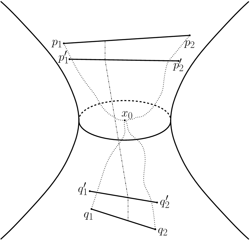
The strategy to prove Theorem 1.B is then the following. Assume there exists a point x0x_{0} with λ⁡(x0)=1−e−v⁡(x0)\lambda(x_{0})=1-e^{-v(x_{0})} very close to 11. We want to show that the width ww is very close to π/2\pi/2. We will first show that the line of curvature of SS corresponding to the positive eigenvalue of SS remains, for a certain amount of time, in the concave side of an umbilical surface Uλ1U_{\lambda_{1}} tangent to SS at x0x_{0}, whose principal curvatures are both equal to λ1=1−e−v(x0)/4\lambda_{1}=1-e^{-v(x_{0})/4}. Such amount of time is finite (in a unit-speed parameterization of the line of curvature), but it can be arranged to tend to infinity as λ⁡(x0)\lambda(x_{0}) tends to 11. This step is basically a maximum principle argument, but requires a technical point to show that the intrinsic acceleration of the line of curvature is also small, i.e. comparable to e−v⁡(x0)e^{-v(x_{0})}.

The surface Uλ1U_{\lambda_{1}} is obtained as the surface at constant timelike distance d1d_{1} from a totally geodesic plane. As λ1\lambda_{1} tends to 11, d1d_{1} tends to π/4\pi/4. By following the line of curvature corresponding to the positive eigenvalue, in the two opposite directions from x0x_{0}, for a time as indicated in the above paragraph, we obtain two points p1p_{1} and p2p_{2}. Moreover p1p_{1} and p2p_{2} converge to ∂∞𝔸​d​𝕊3\partial_{\infty}\mathbb{A}\mathrm{d}\mathbb{S}^{3} as λ⁡(x0)→1\lambda(x_{0})\to 1. Of course analogous statements hold for the two points q1,q2q_{1},q_{2} obtained by following the line of curvature from x0x_{0} corresponding to the negative eigenvalue.

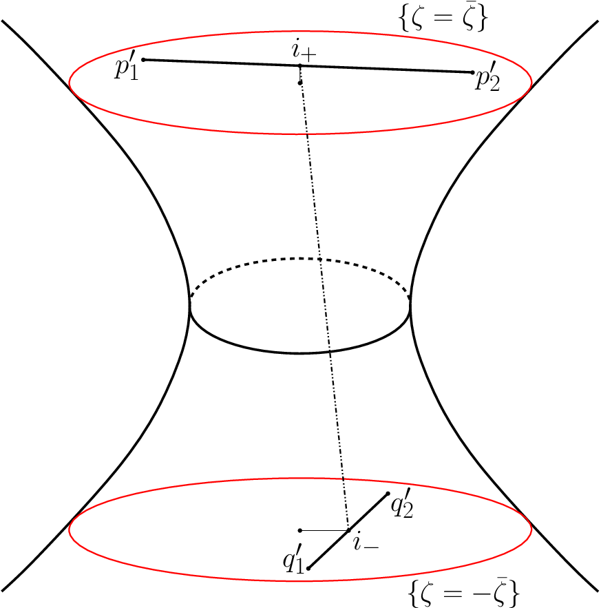
After proving quantitative versions of the above statements, we can give a lower bound for the length of the timelike geodesic segment r1​r2¯\overline{r_{1}r_{2}} which maximizes the distance between the geodesic segments p1​p2¯\overline{p_{1}p_{2}} and q1​q2¯\overline{q_{1}q_{2}}. Since p1​p2¯\overline{p_{1}p_{2}} and q1​q2¯\overline{q_{1}q_{2}} are contained in the convex hull of SS, also r1​r2¯\overline{r_{1}r_{2}} is contained in the convex hull, and therefore the lower bound on the length of r1​r2¯\overline{r_{1}r_{2}} provides a lower bound for the width ww, which only depends on v⁡(x0)=−ln⁡(1−λ⁡(x0))v(x_{0})=-\ln(1-\lambda(x_{0})). The reason why the obtained estimate is efficient when λ⁡(x0)\lambda(x_{0}) approaches 11 is that, in the limit configuration, the lines p1​p2¯\overline{p_{1}p_{2}} and q1​q2¯\overline{q_{1}q_{2}} tend to be in dual position: equivalently, in the limit every point of the first line is connected to every point of the second line by a geodesic timelike segment of length π/2\pi/2. Thus as λ⁡(x0)→1\lambda(x_{0})\to 1, the surface SS is approaching a horospherical surface in a well-quantified fashion.

Organization of the paper

In Section 1, we introduce the necessary notions on Anti-de Sitter space, maximal surfaces and the width, we collect several results proved in [BS10], and finally we give some generalities on quasisymmetric homeomorphisms. In Section 2 we discuss the relation between the cross-ratio norm and the width in Anti-de Sitter space. The main result is Proposition 3.A. Section 3 proves Theorem 1.A, while Section 4 is devoted to the proof of Theorem 1.B. Finally in Section 5 we introduce quasiconformal mappings and minimal Lagrangian extensions, and we prove Theorem 2.A, Theorem 2.B, Proposition 2.C and Corollary 2.D.

Acknowledgements

I am very grateful to Francesco Bonsante, Jean-Marc Schlenker and Mike Wolf for their interest in this work since my first stay at the University of Luxembourg in Spring 2014, for many discussions and advices, and particularly for suggesting (and permitting) that I use in the proof of Proposition 4.B some crucial estimates arisen from a former collaboration of theirs.

Moreover, I would like to thank Dragomir Šarić and Jun Hu for replying to ad-hoc questions about Teichmüller theory in several occasions. Finally, I thank an anonymous referee for several useful comments.

1. Anti-de Sitter space and maximal surfaces

Anti-de Sitter space 𝔸​d​𝕊3\mathbb{A}\mathrm{d}\mathbb{S}^{3} is a pseudo-Riemannian manifold of signature (2,1)(2,1) of constant curvature -1. Consider ℝ2,2{\mathbb{R}}^{2,2}, the vector space ℝ4{\mathbb{R}}^{4} endowed with the bilinear form of signature (2,2):

⟨x,y⟩=x1​y1+x2​y2−x3​y3−x4​y4\langle x,y\rangle=x^{1}y^{1}+x^{2}y^{2}-x^{3}y^{3}-x^{4}y^{4}

and define

𝔸​d​𝕊3^={x∈ℝ2,2:⟨x,x⟩=−1}.\widehat{\mathbb{A}\mathrm{d}\mathbb{S}^{3}}=\left\{x\in{\mathbb{R}}^{2,2}:\langle x,x\rangle=-1\right\}\,.

It turns out that 𝔸​d​𝕊3^\widehat{\mathbb{A}\mathrm{d}\mathbb{S}^{3}} is connected, time-orientable and has the topology of a solid torus. We define Anti-de Sitter space to be the projective domain

𝔸d𝕊3=P({⟨x,x⟩<0})⊂ℝP3,\mathbb{A}\mathrm{d}\mathbb{S}^{3}=\mathrm{P}(\left\{\langle x,x\rangle<0\right\})\subset\mathbb{R}\mathrm{P}^{3}\,,

of which 𝔸​d​𝕊3^\widehat{\mathbb{A}\mathrm{d}\mathbb{S}^{3}} is a double cover. The pseudo-Riemannian metric induced on 𝔸​d​𝕊3^\widehat{\mathbb{A}\mathrm{d}\mathbb{S}^{3}} descends to a metric on 𝔸​d​𝕊3\mathbb{A}\mathrm{d}\mathbb{S}^{3} of constant curvature -1, again time-orientable, which will be denoted again by the product ⟨⋅,⋅⟩\langle\cdot,\cdot\rangle.

The tangent space of 𝔸​d​𝕊3^\widehat{\mathbb{A}\mathrm{d}\mathbb{S}^{3}} at a point xx is Tx​𝔸​d​𝕊3^≅x⟂T_{x}\widehat{\mathbb{A}\mathrm{d}\mathbb{S}^{3}}\cong x^{\perp}. Vectors in tangent spaces are classified according to their causal properties. In particular:

v∈Tx​ℝ2,1​ is ​{​t​i​m​e​l​i​k​eif ​⟨v,v⟩<0​l​i​g​h​t​l​i​k​eif ​⟨v,v⟩=0​s​p​a​c​e​l​i​k​eif ​⟨v,v⟩>0.v\in T_{x}{\mathbb{R}}^{2,1}\text{ is }\begin{cases}\emph{timelike}&\text{if }\langle v,v\rangle<0\\ \emph{lightlike}&\text{if }\langle v,v\rangle=0\\ \emph{spacelike}&\text{if }\langle v,v\rangle>0\end{cases}\,.

Hence, given a spacelike curve γ:I→𝔸​d​𝕊3\gamma:I\to\mathbb{A}\mathrm{d}\mathbb{S}^{3} (i.e. a differentiable curve whose tangent vector at every point is spacelike), we define the length of γ\gamma as

length⁡(γ)=∫I⟨γ˙​(t),γ˙​(t)⟩​𝑑t.\mathrm{length}(\gamma)=\int_{I}\sqrt{\langle\dot{\gamma}(t),\dot{\gamma}(t)\rangle}dt\,.

On the other hand, if γ\gamma is a timelike curve, we still define its length, as

length⁡(γ)=∫I−⟨γ˙​(t),γ˙​(t)⟩​𝑑t.\mathrm{length}(\gamma)=\int_{I}\sqrt{-\langle\dot{\gamma}(t),\dot{\gamma}(t)\rangle}dt\,.

We will fix once and forever a time orientation, so as to talk about future-directed vectors and curves. Our convention is that the vector (0,0,0,1)(0,0,0,1) (based at the point (0,0,1,0)(0,0,1,0)) is future-directed.

The group of isometries of 𝔸​d​𝕊3^\widehat{\mathbb{A}\mathrm{d}\mathbb{S}^{3}} which preserve the orientation and the time-orientation is SO+​(2,2)\mathrm{SO}_{+}(2,2), namely the connected component of the identity in the group of linear isometries of ℝ2,2{\mathbb{R}}^{2,2}. It follows that the group of orientation-preserving, time-preserving isometries of 𝔸​d​𝕊3\mathbb{A}\mathrm{d}\mathbb{S}^{3} is SO+​(2,2)/{±I}\mathrm{SO}_{+}(2,2)/\left\{\pm\mathrm{I}\right\}, and will be denoted simply by Isom⁡(𝔸​d​𝕊3)\mathrm{Isom}(\mathbb{A}\mathrm{d}\mathbb{S}^{3}).

Geodesics of 𝔸​d​𝕊3^\widehat{\mathbb{A}\mathrm{d}\mathbb{S}^{3}} are the intersection of 𝔸​d​𝕊3^\widehat{\mathbb{A}\mathrm{d}\mathbb{S}^{3}} with linear planes of ℝ2,2{\mathbb{R}}^{2,2}. Therefore, geodesics of 𝔸​d​𝕊3\mathbb{A}\mathrm{d}\mathbb{S}^{3} are projective lines which intersect the projective domain 𝔸​d​𝕊3⊂ℝ​P3\mathbb{A}\mathrm{d}\mathbb{S}^{3}\subset\mathbb{R}\mathrm{P}^{3}. It is easy to see that a unit speed parameterization of a spacelike geodesic with initial point pp and initial tangent (spacelike) vector vv is:

(1) γ⁡(t)=[cosh⁡(t)​p+sinh⁡(t)​v],\gamma(t)=[\cosh(t)p+\sinh(t)v]\,,

where the square brackets denote the class in 𝔸​d​𝕊3\mathbb{A}\mathrm{d}\mathbb{S}^{3} of a point of 𝔸​d​𝕊3^\widehat{\mathbb{A}\mathrm{d}\mathbb{S}^{3}}. On the other hand, when vv is a timelike vector, the parameterization of the timelike geodesic is

(2) γ⁡(t)=[cos⁡(t)​p+sin⁡(t)​v].\gamma(t)=[\cos(t)p+\sin(t)v]\,.

Hence timelike geodesics are closed and have length π\pi. Equations (1) and (2) enable to derive immediately the formulae for the length of a spacelike geodesic segment:

(3) cosh⁡(length⁡(p​q¯))=|⟨p,q⟩|,\cosh(\mathrm{length}(\overline{pq}))=|\langle p,q\rangle|\,,

while for a timelike geodesic segment one gets:

(4) cos⁡(length⁡(p​q¯))=|⟨p,q⟩|.\cos(\mathrm{length}(\overline{pq}))=|\langle p,q\rangle|\,.

Analogously, totally geodesic planes of 𝔸​d​𝕊3\mathbb{A}\mathrm{d}\mathbb{S}^{3} are projective planes and are the projection of the intersection of 𝔸​d​𝕊3^\widehat{\mathbb{A}\mathrm{d}\mathbb{S}^{3}} with three-dimensional linear subspaces of ℝ2,2{\mathbb{R}}^{2,2}. There is a duality between totally geodesic planes and points of 𝔸​d​𝕊3\mathbb{A}\mathrm{d}\mathbb{S}^{3}, which is given by associating to a point x∈𝔸​d​𝕊3x\in\mathbb{A}\mathrm{d}\mathbb{S}^{3} the dual plane P=x⟂P=x^{\perp}. One defines

P=x⟂​ is ​{​t​i​m​e​l​i​k​eif ⟨x,x⟩>0(⇔the induced metric is Lorentzian)​l​i​g​h​t​l​i​k​eif ⟨x,x⟩=0(⇔the induced metric is degenerate)​s​p​a​c​e​l​i​k​eif ⟨x,x⟩<0(⇔the induced metric is Riemannian).P=x^{\perp}\text{ is }\begin{cases}\emph{timelike}&\text{if }\langle x,x\rangle>0\quad(\Leftrightarrow\text{the induced metric is Lorentzian})\\ \emph{lightlike}&\text{if }\langle x,x\rangle=0\quad(\Leftrightarrow\text{the induced metric is degenerate})\\ \emph{spacelike}&\text{if }\langle x,x\rangle<0\quad(\Leftrightarrow\text{the induced metric is Riemannian})\end{cases}\,.

Spacelike totally geodesic planes are isometric to the hyperbolic plane ℍ2\mathbb{H}^{2}. Using Equation (4), it is easy to check that the dual plane of a point xx coincides with

x⟂={γ(π/2)|γ:[0,π]→𝔸d𝕊3 is a timelike geodesic ,γ(0)=γ(π)=x}.x^{\perp}=\{\gamma(\pi/2)|\gamma:[0,\pi]\to\mathbb{A}\mathrm{d}\mathbb{S}^{3}\text{ is a timelike geodesic },\gamma(0)=\gamma(\pi)=x\}.

In the affine chart {x4≠0}\left\{x_{4}\neq 0\right\}, 𝔸​d​𝕊3\mathbb{A}\mathrm{d}\mathbb{S}^{3} fills the domain {x2+y2<1+z2}\left\{x^{2}+y^{2}<1+z^{2}\right\}, interior of a one-sheeted hyperboloid; however 𝔸​d​𝕊3\mathbb{A}\mathrm{d}\mathbb{S}^{3} is not contained in a single affine chart, hence in this description we are missing a totally geodesic plane at infinity P∞P_{\infty}, which is the dual plane of the origin. Since geodesics in 𝔸​d​𝕊3\mathbb{A}\mathrm{d}\mathbb{S}^{3} are intersections of 𝔸​d​𝕊3\mathbb{A}\mathrm{d}\mathbb{S}^{3} with linear planes in ℝ2,2{\mathbb{R}}^{2,2}, in the affine chart geodesics are represented by straight lines. See Figure 1.2 for a picture in the affine chart {x4≠0}\left\{x_{4}\neq 0\right\}.

Refer to caption
Figure 1.1. The lightcone of future null geodesic rays from a point and a totally geodesic spacelike plane PP.
Refer to caption
Figure 1.2. Left and right projection from a point ξ∈∂∞𝔸​d​𝕊3\xi\in\partial_{\infty}\mathbb{A}\mathrm{d}\mathbb{S}^{3} to the plane P={x3=0}P=\left\{x_{3}=0\right\}

The boundary at infinity of 𝔸​d​𝕊3\mathbb{A}\mathrm{d}\mathbb{S}^{3} is defined as the topological frontier of 𝔸​d​𝕊3\mathbb{A}\mathrm{d}\mathbb{S}^{3} in ℝ​P3\mathbb{R}\mathrm{P}^{3}, namely the doubly ruled quadric

∂∞𝔸d𝕊3=P({⟨x,x⟩=0}).\partial_{\infty}\mathbb{A}\mathrm{d}\mathbb{S}^{3}=\mathrm{P}(\left\{\langle x,x\rangle=0\right\})\,.

It is naturally endowed with a conformal Lorentzian structure, for which the null lines are precisely the left and right ruling. Given a spacelike plane PP, which we recall is obtained as intersection of 𝔸​d​𝕊3\mathbb{A}\mathrm{d}\mathbb{S}^{3} with a linear hyperplane of ℝ​P3\mathbb{R}\mathrm{P}^{3} and is a copy of ℍ2\mathbb{H}^{2}, PP has a natural boundary at infinity ∂∞(P)\partial_{\infty}(P) which coincides with the usual boundary at infinity of ℍ2\mathbb{H}^{2}. Moreover, PP intersects each line in the left or right ruling in exactly one point. If a spacelike plane PP is chosen, ∂∞𝔸​d​𝕊3\partial_{\infty}\mathbb{A}\mathrm{d}\mathbb{S}^{3} can be identified with ∂∞ℍ2×∂∞ℍ2\partial_{\infty}\mathbb{H}^{2}\times\partial_{\infty}\mathbb{H}^{2} by means of the following description: ξ∈∂∞𝔸​d​𝕊3\xi\in\partial_{\infty}\mathbb{A}\mathrm{d}\mathbb{S}^{3} corresponds to (πl​(ξ),πr​(ξ))(\pi_{l}(\xi),\pi_{r}(\xi)), where πl\pi_{l} and πr\pi_{r} are the projection to ∂∞(P)\partial_{\infty}(P) following the left and right ruling respectively (compare Figure 1.2). Under this identification, the isometry group of 𝔸​d​𝕊3\mathbb{A}\mathrm{d}\mathbb{S}^{3} acts on ∂∞𝔸​d​𝕊3\partial_{\infty}\mathbb{A}\mathrm{d}\mathbb{S}^{3} by projective transformations, and it turns out that

Isom⁡(𝔸​d​𝕊3)≅PSL⁡(2,ℝ)×PSL⁡(2,ℝ).\mathrm{Isom}(\mathbb{A}\mathrm{d}\mathbb{S}^{3})\cong\mathrm{PSL}(2,{\mathbb{R}})\times\mathrm{PSL}(2,{\mathbb{R}})\,.

Given an orientation-preserving homeomorphism ϕ:∂∞ℍ2→∂∞ℍ2\phi:\partial_{\infty}\mathbb{H}^{2}\rightarrow\partial_{\infty}\mathbb{H}^{2}, by means of this identification, the graph of ϕ\phi can be thought of as a curve in ∂∞𝔸​d​𝕊3\partial_{\infty}\mathbb{A}\mathrm{d}\mathbb{S}^{3}, denoted simply by g​r​(ϕ)gr(\phi).

1.1. Maximal surfaces

This paper is concerned with spacelike embedded surfaces in Anti-de Sitter space. A smooth embedded surface σ:S→𝔸​d​𝕊3\sigma:S\rightarrow\mathbb{A}\mathrm{d}\mathbb{S}^{3} is called spacelike if the first fundamental form I⁡(v,w)=⟨d​σ​(v),d​σ​(w)⟩I(v,w)=\langle d\sigma(v),d\sigma(w)\rangle is a Riemannian metric on SS. Equivalently, the tangent plane is a spacelike plane at every point. Let NN be a unit normal vector field to the embedded surface SS. We denote by ∇\nabla and ∇S\nabla^{S} the ambient connection and the Levi-Civita connection of the surface SS, respectively. The second fundamental form of SS is defined as

∇v~w~=∇v~Sw~+I​I​(v,w)​N\nabla_{\tilde{v}}\tilde{w}=\nabla^{S}_{\tilde{v}}\tilde{w}+I\hskip-2.84544ptI(v,w)N

if v~\tilde{v} and w~\tilde{w} are vector fields extending vv and ww. The shape operator is the (1,1)(1,1)-tensor defined as B⁡(v)=∇vNB(v)=\nabla_{v}N. It satisfies the property

I​I​(v,w)=⟨B⁡(v),w⟩.I\hskip-2.84544ptI(v,w)=\langle B(v),w\rangle\,.
Definition 1.1.

A smooth embedded spacelike surface SS in 𝔸​d​𝕊3\mathbb{A}\mathrm{d}\mathbb{S}^{3} is maximal if tr​B=0\mathrm{tr}B=0.

The shape operator is symmetric with respect to the first fundamental form of the surface SS; hence the condition of maximality amounts to the fact that the principal curvatures (namely, the eigenvalues of BB) are opposite at every point.

Definition 1.2.

We say that an embedded spacelike surface SS in 𝔸​d​𝕊3\mathbb{A}\mathrm{d}\mathbb{S}^{3} is entire if it is a compression disc, i.e. it is a topological disc and its frontier is contained in ∂∞𝔸​d​𝕊3\partial_{\infty}\mathbb{A}\mathrm{d}\mathbb{S}^{3}.

The condition that SS is entire is equivalent to the fact that SS can be expressed as a graph over ℍ2\mathbb{H}^{2} in a suitable coordinate system, see [BS10].

An existence result for maximal surfaces in 𝔸​d​𝕊3\mathbb{A}\mathrm{d}\mathbb{S}^{3} was given by Bonsante and Schlenker.

Theorem 1.3 ([BS10]).

Given any orientation-preserving homeomorphism ϕ:ℝ​P1→ℝ​P1\phi:\mathbb{R}\mathrm{P}^{1}\to\mathbb{R}\mathrm{P}^{1}, there exists an entire maximal surface with nonpositive curvature SS in 𝔸​d​𝕊3\mathbb{A}\mathrm{d}\mathbb{S}^{3} such that ∂∞S=g​r​(ϕ)\partial_{\infty}S=gr(\phi).

Observe that, by the Gauss equation in 𝔸​d​𝕊3\mathbb{A}\mathrm{d}\mathbb{S}^{3}, the curvature of the induced metric on the maximal surface SS is −1+λ2-1+\lambda^{2}, where λ\lambda and −λ-\lambda are the principal curvatures. Hence the condition of nonpositive curvature corresponds to the fact that the principal curvatures of SS are in [−1,1][-1,1].

1.2. Width of convex hulls

Since 𝔸​d​𝕊3\mathbb{A}\mathrm{d}\mathbb{S}^{3} is a projective geometry, we have a well-defined notion of convexity. In particular, we can give the definition of convex hull of a curve in ∂∞𝔸​d​𝕊3\partial_{\infty}\mathbb{A}\mathrm{d}\mathbb{S}^{3}.

Definition 1.4.

Given a curve Γ=g​r​(ϕ)\Gamma=gr(\phi) in ∂∞𝔸​d​𝕊3\partial_{\infty}\mathbb{A}\mathrm{d}\mathbb{S}^{3}, the convex hull of Γ\Gamma, which we denote by 𝒞​ℋ​(Γ)\mathcal{CH}(\Gamma), is the intersection of half-spaces bounded by planes PP such that ∂∞P\partial_{\infty}P does not intersect Γ\Gamma, and the half-space is taken on the side of PP containing Γ\Gamma.

It can be proved that the convex hull of Γ\Gamma, which is well-defined in ℝ​P3\mathbb{R}\mathrm{P}^{3}, is contained in 𝔸​d​𝕊3∪∂∞𝔸​d​𝕊3\mathbb{A}\mathrm{d}\mathbb{S}^{3}\cup\partial_{\infty}\mathbb{A}\mathrm{d}\mathbb{S}^{3}, and is actually contained in an affine chart.

Let us fix a totally geodesic spacelike plane QQ (for instance, the plane {x4=0}\left\{x_{4}=0\right\}, which is the plane at infinity in Figure 1.2). We will denote by d𝔸​d​𝕊3​(⋅,⋅)d_{\mathbb{A}\mathrm{d}\mathbb{S}^{3}}(\cdot,\cdot) the timelike distance in 𝔸​d​𝕊3∖Q\mathbb{A}\mathrm{d}\mathbb{S}^{3}\setminus Q, which is defined as follows.

Definition 1.5.

Given points pp and qq which are connected by a timelike curve, the timelike distance between pp and qq is

d𝔸​d​𝕊3(p,q)=supγ{length(γ)|γ:[0,1]→𝔸d𝕊3∖Q is a timelike curve, γ(0)=p,γ(1)=q}.d_{\mathbb{A}\mathrm{d}\mathbb{S}^{3}}(p,q)=\sup_{\gamma}\{\mathrm{length(\gamma)}|\gamma:[0,1]\to\mathbb{A}\mathrm{d}\mathbb{S}^{3}\setminus Q\text{ is a timelike curve, }\gamma(0)=p,\gamma(1)=q\}\,.

The distance between two such points p,qp,q is achieved along the timelike geodesic connecting pp and qq. The timelike distance satisfies the reverse triangle inequality, meaning that,

d𝔸​d​𝕊3​(p,r)≥d𝔸​d​𝕊3​(p,q)+d𝔸​d​𝕊3​(q,r),d_{\mathbb{A}\mathrm{d}\mathbb{S}^{3}}(p,r)\geq d_{\mathbb{A}\mathrm{d}\mathbb{S}^{3}}(p,q)+d_{\mathbb{A}\mathrm{d}\mathbb{S}^{3}}(q,r)\,,

provided both pairs (p,q)(p,q) and (q,r)(q,r) are connected by a timelike curve. In a completely analogous way, we define the distance of a point xx from a totally geodesic spacelike plane PP as the supremum of the length of a timelike curve connecting xx to PP.

We are now ready to introduce the notion of width of the convex hull, as defined in [BS10].

Definition 1.6.

Given a curve Γ=g​r​(ϕ)\Gamma=gr(\phi) in ∂∞𝔸​d​𝕊3\partial_{\infty}\mathbb{A}\mathrm{d}\mathbb{S}^{3}, the width ww of the convex hull 𝒞​ℋ​(Γ)\mathcal{CH}(\Gamma) is the supremum of the length of a timelike geodesic contained in 𝒞​ℋ​(Γ)\mathcal{CH}(\Gamma).

Remark 1.7.

Note that the distance d𝔸​d​𝕊3​(p,q)d_{\mathbb{A}\mathrm{d}\mathbb{S}^{3}}(p,q) is achieved along the geodesic timelike segment connecting pp and qq. Hence Definition 1.6 is equivalent to

(5) w=supp∈∂−𝒞,q∈∂+𝒞d𝔸​d​𝕊3​(p,q),w=\sup_{p\in\partial_{-}\mathcal{C},q\in\partial_{+}\mathcal{C}}d_{\mathbb{A}\mathrm{d}\mathbb{S}^{3}}(p,q)\,,

where 𝒞=𝒞​ℋ​(Γ)\mathcal{C}=\mathcal{CH}(\Gamma) and ∂±𝒞\partial_{\pm}\mathcal{C} denote the two components (one future and one past component) of the boundary of the convex hull of Γ\Gamma in 𝔸​d​𝕊3\mathbb{A}\mathrm{d}\mathbb{S}^{3}.

In particular, we note that

(6) w=supx∈𝒞(d𝔸​d​𝕊3​(x,∂−𝒞)+d𝔸​d​𝕊3​(x,∂+𝒞)).w=\sup_{x\in\mathcal{C}}\left(d_{\mathbb{A}\mathrm{d}\mathbb{S}^{3}}(x,\partial_{-}\mathcal{C})+d_{\mathbb{A}\mathrm{d}\mathbb{S}^{3}}(x,\partial_{+}\mathcal{C})\right).

To stress once more the meaning of this equality, note that the supremum in (6) cannot be achieved on a point xx such that the two segments realizing the distance from xx to ∂−𝒞\partial_{-}\mathcal{C} and ∂+𝒞\partial_{+}\mathcal{C} are not part of a unique geodesic line. Indeed, if at xx the two segments form an angle, the piecewise geodesic can be made longer by avoiding the point xx, as in Figure 1.3. We also remark that if the distance between a point xx and ∂±𝒞\partial_{\pm}\mathcal{C} is achieved along a geodesic segment ll, then the maximality condition imposes that ll must be orthogonal to a support plane to ∂±𝒞\partial_{\pm}\mathcal{C} at ∂±𝒞∩l\partial_{\pm}\mathcal{C}\cap l.

Refer to caption
Figure 1.3. A path through xx which is not geodesic does not achieve the maximum distance.

1.3. An application of the maximum principle

A key property used in this paper is that maximal surfaces with boundary at infinity a curve Γ=g​r​(ϕ)\Gamma=gr(\phi) are contained in the convex hull of Γ\Gamma. Although this fact is known, we prove it here by applying maximum principle to a simple linear PDE describing maximal surfaces.

Hereafter Hess​u\mathrm{Hess}\,u denotes the Hessian of a smooth function uu on the surface SS, i.e. the (1,1) tensor

Hess​u​(v)=∇vS​grad⁡u.\mathrm{Hess}\,u(v)=\nabla^{S}_{v}\operatorname{grad}u\,.

Finally, ΔS\Delta_{S} denotes the Laplace-Beltrami operator of SS, which can be defined as

ΔS​u=tr⁡(Hess​u).\Delta_{S}u=\mathrm{tr}(\mathrm{Hess}\,u)\,.

Proposition 1.8 was proved in [BS10]. We give a proof here for the sake of completeness. We first observe that, given a point xx and a totally geodesic spacelike plane PP, it is easy to check (as for Equations (3) and (4)) that the timelike distance d𝔸​d​𝕊3​(x,P)d_{\mathbb{A}\mathrm{d}\mathbb{S}^{3}}(x,P) of xx from P=p⟂P=p^{\perp} satisfies

sin⁡d𝔸​d​𝕊3​(x,P)=|⟨x,p⟩|.\sin d_{\mathbb{A}\mathrm{d}\mathbb{S}^{3}}(x,P)=|\langle x,p\rangle|\,.
Proposition 1.8.

Given a maximal surface S⊂𝔸​d​𝕊3S\subset\mathbb{A}\mathrm{d}\mathbb{S}^{3} and a plane PP, let u:S→ℝu:S\rightarrow{\mathbb{R}} be the function u⁡(x)=sin⁡d𝔸​d​𝕊3​(x,P)u(x)=\sin d_{\mathbb{A}\mathrm{d}\mathbb{S}^{3}}(x,P), where d𝔸​d​𝕊3​(x,P)d_{\mathbb{A}\mathrm{d}\mathbb{S}^{3}}(x,P) is considered as a signed distance. Let NN be the future unit normal to SS and B=∇NB=\nabla N the shape operator. Then

(7) Hess​u−u​E=1−u2+‖grad⁡u‖2​B,\mathrm{Hess}\,u-u\,E=\sqrt{1-u^{2}+||\operatorname{grad}u||^{2}}B~,

where EE denotes the identity operator. As a consequence, uu satisfies the linear equation

(L) ΔS​u−2​u=0.\Delta_{S}u-2u=0\,.
Proof.

Let us assume that PP is the plane dual to the point p∈𝔸​d​𝕊3p\in\mathbb{A}\mathrm{d}\mathbb{S}^{3}. We will perform the computation in the double cover 𝔸​d​𝕊3^\widehat{\mathbb{A}\mathrm{d}\mathbb{S}^{3}}. Then uu is the restriction to SS of the function UU defined by:

(8) U⁡(x)=sin⁡d𝔸​d​𝕊3​(x,P)=⟨x,p⟩.U(x)=\sin d_{\mathbb{A}\mathrm{d}\mathbb{S}^{3}}(x,P)=\langle x,p\rangle\,.

Let NN be the unit normal vector field to SS; we compute grad⁡u\operatorname{grad}u by projecting the gradient ∇U\nabla U of UU to the tangent plane to SS:

(9) ∇U=p+⟨p,x⟩​x\displaystyle\nabla U=p+\langle p,x\rangle x
(10) grad⁡u⁡(x)=p+⟨p,x⟩​x+⟨p,N⟩​N\displaystyle\operatorname{grad}u(x)=p+\langle p,x\rangle x+\langle p,N\rangle N

Now Hess​u​(v)=∇vS​grad⁡u\mathrm{Hess}\,u(v)=\nabla^{S}_{v}\operatorname{grad}u, where ∇S\nabla^{S} is the Levi-Civita connection of SS, namely the projection of the flat connection of ℝ2,2{\mathbb{R}}^{2,2}, and so for any v∈Tx​𝔸​d​𝕊3^v\in T_{x}\widehat{\mathbb{A}\mathrm{d}\mathbb{S}^{3}} one gets:

Hess​u​(v)=⟨p,x⟩​v+⟨p,N⟩​∇vSN=u⁡(x)​v+⟨∇U,N⟩​B​(v).\mathrm{Hess}\,u(v)=\langle p,x\rangle v+\langle p,N\rangle\nabla^{S}_{v}N=u(x)v+\langle\nabla U,N\rangle B(v)\,.

Moreover, ∇U=grad⁡u+⟨∇U,N⟩​N\nabla U=\operatorname{grad}u+\langle\nabla U,N\rangle N and thus

(11) ⟨∇U,N⟩2=‖grad⁡u‖2−⟨∇U,∇U⟩=1−u2+‖grad⁡u‖2,\langle\nabla U,N\rangle^{2}=||\operatorname{grad}u||^{2}-\langle\nabla U,\nabla U\rangle=1-u^{2}+||\operatorname{grad}u||^{2}\,,

which proves (7). By taking the trace, (L) follows. ∎

Corollary 1.9.

Let SS be an entire maximal surface in 𝔸​d​𝕊3\mathbb{A}\mathrm{d}\mathbb{S}^{3}. Then SS is contained in the convex hull of ∂∞S\partial_{\infty}S.

Proof.

If Γ=∂∞S\Gamma=\partial_{\infty}S is a circle, then SS is a totally geodesic plane which coincides with the convex hull of Γ\Gamma. Hence we can suppose Γ\Gamma is not a circle. Consider a plane P−P_{-} which does not intersect Γ\Gamma and the function uu defined as in Equation (8) in Proposition 1.8, with respect to P−P_{-}. Suppose their mutual position is such that u≥0u\geq 0 in the region of SS close to the boundary at infinity (i.e. in the complement of a large compact set). If there exists some point where u<0u<0, then by Equation (L) at a minimum point ΔS​u=2​u<0\Delta_{S}u=2u<0, which gives a contradiction. The proof is analogous for a plane P+P_{+} on the other side of Γ\Gamma, by switching the signs. This shows that every convex set containing Γ\Gamma contains also SS. ∎

1.4. Two opposite examples

We report here the two examples to have in mind for our study of maximal surface. The first is a very simple example, namely a totally geodesic plane, for which the principal curvatures vanish at every point. To some extent, the second example can be considered as the opposite of a totally geodesic plane, since in the second case the principal curvatures are 11 and −1-1 at every point.

Example 1.10.

(Totally geodesic planes) By definition, a totally geodesic plane PP has shape operator B≡0B\equiv 0. Hence a totally geodesic plane is a maximal surface, and ∂∞P=g​r​(A)\partial_{\infty}P=gr(A), where A∈PSL⁡(2,ℝ)A\in\mathrm{PSL}(2,{\mathbb{R}}) is the trace on ℝ​P1=∂∞ℍ2\mathbb{R}\mathrm{P}^{1}=\partial_{\infty}\mathbb{H}^{2} of an isometry of ℍ2\mathbb{H}^{2}. Hence the width of the convex hull vanishes. It is also easy to see that, given a curve in ∂∞𝔸​d​𝕊3\partial_{\infty}\mathbb{A}\mathrm{d}\mathbb{S}^{3}, if w=0w=0 then the curve is necessarily the boundary of a totally geodesic plane. Therefore the unique maximal surface with zero width (up to isometries of 𝔸​d​𝕊3\mathbb{A}\mathrm{d}\mathbb{S}^{3}) is a totally geodesic plane.

Example 1.11.

(Horospherical surfaces) Consider a spacelike line ll in 𝔸​d​𝕊3\mathbb{A}\mathrm{d}\mathbb{S}^{3}. The dual line l⟂l^{\perp} is obtained as the intersection of all totally geodesic planes dual to points of ll. Recall that timelike geodesics in 𝔸​d​𝕊3\mathbb{A}\mathrm{d}\mathbb{S}^{3} are closed and have length π\pi. Hence one equivalently has:

l⟂={γ(π/2)|γ:[0,π]→𝔸d𝕊3 is a timelike geodesic ,γ(0)=γ(π)∈l}.l^{\perp}=\{\gamma(\pi/2)|\gamma:[0,\pi]\to\mathbb{A}\mathrm{d}\mathbb{S}^{3}\text{ is a timelike geodesic },\gamma(0)=\gamma(\pi)\in l\}\,.

Let us define the smooth surface

H={γ(π/4)|γ:[0,π/2]→𝔸d𝕊3 is a future-directed timelike geodesic,γ(0)∈l,γ(π/2)∈l⟂}.H=\{\gamma(\pi/4)|\gamma:[0,\pi/2]\to\mathbb{A}\mathrm{d}\mathbb{S}^{3}\text{ is a future-directed timelike geodesic},\gamma(0)\in l,\gamma(\pi/2)\in l^{\perp}\}\,.

See Figure 1.4 for a schematic picture.

The group of isometries which preserve ll (and thus preserves also l⟂l^{\perp}) is isomorphic to ℝ×ℝ{\mathbb{R}}\times{\mathbb{R}}, where ℝ×{0}{\mathbb{R}}\times\{0\} fixes ll pointwise and acts on l⟂l^{\perp} by translation (it actually acts as a rotation around the spacelike line ll), while {0}×ℝ\{0\}\times{\mathbb{R}} does the opposite. The induced metric on HH is flat, and thus HH is isometric to the Euclidean plane. Moreover, for every point x∈Hx\in H, the surface HH has an orientation-reversing, time-reversing isometry obtained by reflection in a plane PP tangent to a point x∈Hx\in H, followed by rotation of angle π/2\pi/2 around the timelike geodesic orthogonal to PP at xx. This basically shows that the principal curvatures λ1,λ2\lambda_{1},\lambda_{2} of HH are necessarily opposite to one another, hence HH is a maximal surface. Moreover, since by the Gauss equation

0=KH=−1−λ1​λ2=−1+λ2,0=K_{H}=-1-\lambda_{1}\lambda_{2}=-1+\lambda^{2}\,,

it follows that the principal curvatures are necessarily ±1\pm 1 at every point. Finally, by construction, the width of the convex hull of HH is precisely π/2\pi/2.

Refer to caption
Refer to caption
Figure 1.4. A subset of a horospherical surface. The lines of curvature provide Euclidean coordinates for the induced metric, and are planar curves parallel to ll or l⟂l^{\perp}. The boundary at infinity is composed of four lightlike segments.

Bonsante and Schlenker proved an important property of rigidity of maximal surfaces with large principal curvatures.

Lemma 1.12 ([BS10, Lemma 5.5]).

Given a maximal surface SS in 𝔸​d​𝕊3\mathbb{A}\mathrm{d}\mathbb{S}^{3} with nonpositive curvature, if the curvature is 00 at some point, then SS is a subset of a horospherical surface.

The proof of Lemma 1.12 follows from applying the maximum principle to Equation (Q), which is stated in the following lemma. Recall that an umbilical point on a surface is a point where the two principal curvatures are equal. Hence for a maximal surface, umbilical points are the points where the principal curvatures vanish.

Lemma 1.13 ([KS07, Lemma 3.11]).

Given a maximal surface SS in 𝔸​d​𝕊3\mathbb{A}\mathrm{d}\mathbb{S}^{3}, with principal curvatures ±λ\pm\lambda, let χ:S→ℝ\chi:S\to{\mathbb{R}} be the function defined (in the complement of umbilical points) by χ=−ln⁡|λ|\chi=-\ln|\lambda|. Then χ\chi satisfies the quasi-linear equation

(Q) ΔS​χ=2​(1−e−2​χ).\Delta_{S}\chi=2(1-e^{-2\chi})\,.

1.5. Uniformly negative curvature

As a warm-up for what will come next, we give here a proof of Proposition 1.C. Our proof was basically already implicit in [BS10, Claim 3.21], and will be a consequence of the following easy lemma, which we prove here by completeness. See also [KS07].

Lemma 1.14.

Given a smooth spacelike surface SS in 𝔸​d​𝕊3\mathbb{A}\mathrm{d}\mathbb{S}^{3}, let SρS_{\rho} be the surface at timelike distance ρ\rho from SS, obtained by following the normal flow. Then the pull-back to SS of the induced metric on the surface SρS_{\rho} is given by

(12) Iρ=I((cos(ρ)E+sin(ρ)B)⋅,(cos(ρ)E+sin(ρ)B)⋅).I_{\rho}=I((\cos(\rho)E+\sin(\rho)B)\cdot,(\cos(\rho)E+\sin(\rho)B)\cdot)\,.

The second fundamental form and the shape operator of SρS_{\rho} are given by

(13) IIρ=I((−sin(ρ)E+cos(ρ)B)⋅,(cos(ρ)E−sin(ρ)B)⋅),\displaystyle I\hskip-2.84544ptI_{\rho}=I((-\sin(\rho)E+\cos(\rho)B)\cdot,(\cos(\rho)E-\sin(\rho)B)\cdot)\,,
(14) Bρ=(cos⁡(ρ)​E+sin⁡(ρ)​B)−1​(−sin⁡(ρ)​E+cos⁡(ρ)​B).\displaystyle B_{\rho}=(\cos(\rho)E+\sin(\rho)B)^{-1}(-\sin(\rho)E+\cos(\rho)B)\,.
Proof.

Let σ\sigma be a smooth embedding of the maximal surface SS, with oriented unit normal NN. The geodesics orthogonal to SS at a point x=σ⁡(y)x=\sigma(y) can be written as

γx​(ρ)=cos⁡(ρ)​σ​(y)+sin⁡(ρ)​N​(x).\gamma_{x}(\rho)=\cos(\rho)\sigma(y)+\sin(\rho)N(x)\,.

Then we compute

Iρ​(v,w)=\displaystyle I_{\rho}(v,w)= ⟨d​γx​(ρ)​(v),d​γx​(ρ)​(w)⟩\displaystyle\langle d\gamma_{x}(\rho)(v),d\gamma_{x}(\rho)(w)\rangle
=\displaystyle= ⟨cos⁡(ρ)​d​σx​(v)+sin⁡(ρ)​d​(N∘σ)x​(v),cos⁡(r)​d​σx​(w)+sin⁡(ρ)​d​(N∘σ)x​(w)⟩\displaystyle\langle\cos(\rho)d\sigma_{x}(v)+\sin(\rho)d(N\circ\sigma)_{x}(v),\cos(r)d\sigma_{x}(w)+\sin(\rho)d(N\circ\sigma)_{x}(w)\rangle
=\displaystyle= I⁡(cos⁡(ρ)​v+sin⁡(ρ)​B​(v),cos⁡(ρ)​w+sin⁡(ρ)​B​(w)).\displaystyle I(\cos(\rho)v+\sin(\rho)B(v),\cos(\rho)w+\sin(\rho)B(w))\,.

We have used the equation B=∇NB=\nabla N. The formula for the second fundamental form follows from the fact that I​Iρ=12​d​Iρd​ρI\hskip-2.84544ptI_{\rho}=\frac{1}{2}\frac{dI_{\rho}}{d\rho}, and the formula for BρB_{\rho} from equating Bρ=Iρ−1​I​IρB_{\rho}=I_{\rho}^{-1}I\hskip-2.84544ptI_{\rho}. ∎

It follows that, if the principal curvatures of a maximal surface SS are λ1=λ∈[0,1)\lambda_{1}=\lambda\in[0,1) and λ2=−λ\lambda_{2}=-\lambda, then the principal curvatures of SρS_{\rho} are

λρ=λ−tan⁡(ρ)1+λ​tan⁡(ρ)=tan⁡(ρ0−ρ),\lambda_{\rho}=\frac{\lambda-\tan(\rho)}{1+\lambda\tan(\rho)}=\tan(\rho_{0}-\rho)\,,

where tan⁡ρ0=λ\tan\rho_{0}=\lambda, and

λρ′=−λ−tan⁡(−ρ)1−λ​tan⁡(ρ)=tan⁡(−ρ0−ρ).\lambda^{\prime}_{\rho}=\frac{-\lambda-\tan(-\rho)}{1-\lambda\tan(\rho)}=\tan(-\rho_{0}-\rho)\,.

In particular λρ\lambda_{\rho} and λρ′\lambda^{\prime}_{\rho} are non-singular for every ρ\rho between −π/4-\pi/4 and π/4\pi/4. It then turns out that SρS_{\rho} is convex at every point for ρ<−‖ρ0‖∞\rho<-||\rho_{0}||_{\infty}, and concave for ρ>‖ρ0‖∞\rho>||\rho_{0}||_{\infty}. This proves that the width ww is less than 2​‖ρ0‖∞=2​arctan||λ||∞2||\rho_{0}||_{\infty}=2\arctan||\lambda||_{\infty}. Therefore

tan⁡(ω2)≤‖λ‖∞,\tan\left(\frac{\omega}{2}\right)\leq||\lambda||_{\infty}\,,

and the statement of Proposition 1.C follows.

Proposition 1.C.

Let SS be an entire maximal surface in 𝔸​d​𝕊3\mathbb{A}\mathrm{d}\mathbb{S}^{3} with ‖λ‖∞<1||\lambda||_{\infty}<1 and let ww be the width of the convex hull. Then

tan⁡w≤2​‖λ‖∞1−‖λ‖∞2.\tan w\leq\frac{2||\lambda||_{\infty}}{1-||\lambda||_{\infty}^{2}}\,.

A direct consequence is that, if SS is an entire maximal surface with uniformly negative curvature (equivalently, with ‖λ‖∞<1||\lambda||_{\infty}<1), then w<π/2w<\pi/2, see also [BS10, Corollary 3.22]. Also the converse holds:

Proposition 1.15 ([BS10]).

Given any entire maximal surface SS of nonpositive curvature in 𝔸​d​𝕊3\mathbb{A}\mathrm{d}\mathbb{S}^{3}, the width ww of the convex hull of SS is at most π/2\pi/2. Moreover, w<π/2w<\pi/2 if and only if SS has uniformly negative curvature.

The proof of the converse implication in [BS10] used quasisymmetric homemorphisms (see below) and minimal Lagrangian extensions (which will be discussed in Section 5). Observe that our Theorem 1.B gives a quantitative version of the converse implication of Proposition 1.15.

1.6. Quasisymmetric homeomorphisms of the circle

Given an orientation-preserving homeomorphism ϕ:ℝ​P1→ℝ​P1\phi:\mathbb{R}\mathrm{P}^{1}\to\mathbb{R}\mathrm{P}^{1}, we define the cross-ratio norm of ϕ\phi as

‖ϕ‖c​r=supc​r​(Q)=−1|ln⁡|c​r​(ϕ⁡(Q))||,||\phi||_{cr}=\sup_{cr(Q)=-1}\left|\ln\left|cr(\phi(Q))\right|\right|\,,

where Q=(z1,z2,z3,z4)Q=(z_{1},z_{2},z_{3},z_{4}) is any quadruple of points on ℝ​P1\mathbb{R}\mathrm{P}^{1} and we use the following definition of cross-ratio:

c​r​(z1,z2,z3,z4)=(z4−z1)​(z3−z2)(z2−z1)​(z3−z4).cr(z_{1},z_{2},z_{3},z_{4})=\frac{(z_{4}-z_{1})(z_{3}-z_{2})}{(z_{2}-z_{1})(z_{3}-z_{4})}.

According to this definition, a quadruple Q=(z1,z2,z3,z4)Q=(z_{1},z_{2},z_{3},z_{4}) is symmetric (i.e. the hyperbolic geodesics connecting z1z_{1} to z3z_{3} and z2z_{2} to z4z_{4} intersect orthogonally) if and only if c​r​(Q)=−1cr(Q)=-1.

Observe that ‖ϕ‖c​r∈[0,∞]||\phi||_{cr}\in[0,\infty] and ‖ϕ‖c​r=0||\phi||_{cr}=0 if and only if ϕ\phi is a projective transformation, i.e. ϕ∈PSL⁡(2,ℝ)\phi\in\mathrm{PSL}(2,{\mathbb{R}}). Indeed, by post-composing with a projective transformation, one can assume that ϕ\phi fixes three points of ℝ​P1\mathbb{R}\mathrm{P}^{1}, and then the conclusion is straightforward. A homeomorphism is quasisymmetric when it has finite cross-ratio norm:

Definition 1.16.

An orientation-preserving homeomorphism ϕ:ℝ​P1→ℝ​P1\phi:\mathbb{R}\mathrm{P}^{1}\to\mathbb{R}\mathrm{P}^{1} is quasisymmetric if and only if ‖ϕ‖c​r<+∞||\phi||_{cr}<+\infty.

Quasisymmetric homeomorphisms arise naturally in the context of quasiconformal mappings and universal Teichmüller space, which is actually one of the main themes of this paper. However, we defer the introduction of this point of view to Section 5, where some applications are given.

The first intimate correlation between the cross-ratio norm of a quasisymmetric homeomorphism ϕ\phi and the width of the convex hull of g​r​(ϕ)gr(\phi) was proved in [BS10]:

Theorem 1.17 ([BS10, Theorem 1.12]).

Given any orientation-preserving homeomorphism ϕ:ℝ​P1→ℝ​P1\phi:\mathbb{R}\mathrm{P}^{1}\to\mathbb{R}\mathrm{P}^{1}, let ww be the width of the convex hull of g​r​(ϕ)gr(\phi). Then w<π/2w<\pi/2 if and only if ϕ\phi is quasisymmetric.

Again, Proposition 3.A will provide a more precise version of Theorem 1.17, giving a quantitative inequality between the width and the cross-ratio norm.

Remark 1.18.

Actually, Theorem 1.17 holds under a more general hypothesis, namely for more general curves in ∂∞𝔸​d​𝕊3\partial_{\infty}\mathbb{A}\mathrm{d}\mathbb{S}^{3}, which, roughly speaking, may also contain lightlike segments. We will not be interested in these objects in this paper.

A refinement of Theorem 1.3 was given in [BS10] under the assumption that the curve at infinity is the graph of a quasisymmetric homeomorphism.

Theorem 1.19 ([BS10]).

Given any quasisymmetric homeomorphism ϕ:ℝ​P1→ℝ​P1\phi:\mathbb{R}\mathrm{P}^{1}\rightarrow\mathbb{R}\mathrm{P}^{1}, there exists a unique entire maximal surface SS in 𝔸​d​𝕊3\mathbb{A}\mathrm{d}\mathbb{S}^{3} with uniformly negative curvature such that ∂∞S=g​r​(ϕ)\partial_{\infty}S=gr(\phi).

1.7. Compactness properties

One of the main tools used in [BS10] is a result of compactness for maximal surfaces in 𝔸​d​𝕊3\mathbb{A}\mathrm{d}\mathbb{S}^{3}. To conclude the preliminaries of this paper, we briefly discuss some properties of compactness for maximal surfaces and quasisymmetric homeomorphisms.

Given a spacelike plane P0P_{0} in 𝔸​d​𝕊3\mathbb{A}\mathrm{d}\mathbb{S}^{3} and a point x0∈P0x_{0}\in P_{0}, let ll be the timelike geodesic through x0x_{0} orthogonal to P0P_{0}. We define the solid cylinder C​l​(x0,P0,R0)Cl(x_{0},P_{0},R_{0}) of radius R0R_{0} above P0P_{0} centered at x0x_{0} as the set of points x∈𝔸​d​𝕊3x\in\mathbb{A}\mathrm{d}\mathbb{S}^{3} which lie on a spacelike plane PxP_{x} orthogonal to ll such that dPx​(x,l∩Px)≤R0d_{P_{x}}(x,l\cap P_{x})\leq R_{0}. See also Figure 1.5.

Refer to caption
Refer to caption
Figure 1.5. The definition of the solid cylinder C​l​(x0,P0,R0)Cl(x_{0},P_{0},R_{0}). On the right, its intersection with the future and past lightcone over x0x_{0}.

The solid cylinder C​l​(x0,P0,R0)Cl(x_{0},P_{0},R_{0}) can also be conveniently described in the following way. Assuming (in the double cover 𝔸​d​𝕊3^\widehat{\mathbb{A}\mathrm{d}\mathbb{S}^{3}}, for one moment) that x0=(0,0,1,0)x_{0}=(0,0,1,0) and the normal vector to P0P_{0} is N0=(0,0,0,1)N_{0}=(0,0,0,1), let us consider the following coordinate system:

(15) (r,θ,ζ)↦[cos⁡θ​sinh⁡r,sin⁡θ​sinh⁡r,cos⁡ζ​cosh⁡r,sin⁡ζ​cosh⁡r],(r,\theta,\zeta)\mapsto[\cos\theta\sinh r,\sin\theta\sinh r,\cos\zeta\cosh r,\sin\zeta\cosh r]\,,

defined for r∈ℝ,θ∈S1,ζ∈S1r\in{\mathbb{R}},\theta\in S^{1},\zeta\in S^{1}. This means that the level sets with ζ=c\zeta=c are totally geodesic planes orthogonal to the timelike line

{[0,0,cos⁡ζ,sin⁡ζ]:ζ∈S1},\{[0,0,\cos\zeta,\sin\zeta]:\zeta\in S^{1}\}\,,

which passes through the point x0=(0,0,1,0)x_{0}=(0,0,1,0) with future-directed normal N0=(0,0,0,1)N_{0}=(0,0,0,1). It is easy to see that, by this description, the solid cylinder C​l​(x0,P0,R0)Cl(x_{0},P_{0},R_{0}) is determined by the relation r≤R0r\leq R_{0}.

From the tools in the paper [BS10], the following lemma is proved:

Lemma 1.20.

Given a spacelike plane P0P_{0} and a point x0∈P0x_{0}\in P_{0}, every sequence SnS_{n} of entire maximal surfaces with nonpositive curvature, tangent to P0P_{0} at x0x_{0}, admits a subsequence converging C∞C^{\infty} to an entire maximal surface on the solid cylinders C​l​(x0,P0,R)Cl(x_{0},P_{0},R), for every R>0R>0.

A somehow similar property of compactness for quasisymmetric homeomorphisms will be used in several occasions. See also [BZ06] for a discussion.

Theorem 1.21.

Let k>0k>0 and ϕn:ℝ​P1→ℝ​P1\phi_{n}:\mathbb{R}\mathrm{P}^{1}\to\mathbb{R}\mathrm{P}^{1} be a family of orientation-preserving quasisymmetric homeomorphisms of the circle, with ‖ϕn‖c​r≤k||\phi_{n}||_{cr}\leq k. Then there exists a subsequence ϕnk\phi_{n_{k}} for which one of the following holds:

  • •

    The homeomorphisms ϕnk\phi_{n_{k}} converge uniformly to a quasisymmetric homeomorphism ϕ:ℝ​P1→ℝ​P1\phi:\mathbb{R}\mathrm{P}^{1}\to\mathbb{R}\mathrm{P}^{1}, with ‖ϕ‖c​r≤k||\phi||_{cr}\leq k;

  • •

    The homeomorphisms ϕnk\phi_{n_{k}} converge uniformly on the complement of any open neighborhood of a point of ℝ​P1\mathbb{R}\mathrm{P}^{1} to a constant map c:ℝ​P1→ℝ​P1c:\mathbb{R}\mathrm{P}^{1}\to\mathbb{R}\mathrm{P}^{1}.

Remark 1.22.

It is also not difficult to prove that, given a sequence of entire maximal surfaces SnS_{n} which converges uniformly on compact cylinders C​l​(x0,P0,R)Cl(x_{0},P_{0},R) to an entire maximal surface S∞S_{\infty}, then the asymptotic boundaries ∂∞Sn\partial_{\infty}S_{n} converge (in the Hausdorff convergence, for instance) to the asymptotic boundary ∂∞S∞\partial_{\infty}S_{\infty} of the limit surface.

2. Cross-ratio norm and the width of the convex hull

The purpose of this section is to investigate the relation between the width of the convex hull of g​r​(ϕ)gr(\phi) and the cross-ratio norm of ϕ\phi when ϕ\phi is a quasisymmetric homeomorphism. The main result is thus Proposition 3.A. To some extent, Proposition 3.A is a quantitative version of Theorem 1.17.

Proposition 3.A.

Given any quasisymmetric homeomorphism ϕ\phi of ℝ​P1\mathbb{R}\mathrm{P}^{1}, let ww be the width of the convex hull of the graph of ϕ\phi in ∂∞𝔸​d​𝕊3\partial_{\infty}\mathbb{A}\mathrm{d}\mathbb{S}^{3}. Then

(16) tan⁡(w)≤sinh⁡(‖ϕ‖c​r2).\tan(w)\leq\sinh{\left(\frac{||\phi||_{cr}}{2}\right)}\,.
Proof.

To prove the upper bound on the width, suppose the width of the convex hull 𝒞\mathcal{C} of g​r​(ϕ)gr(\phi) is w∈(0,π/2)w\in(0,\pi/2). Let k=‖ϕ‖c​rk=||\phi||_{cr}. We can find a sequence of pairs (pn,qn)(p_{n},q_{n}) such that d𝔸​d​𝕊3​(pn,qn)↗wd_{\mathbb{A}\mathrm{d}\mathbb{S}^{3}}(p_{n},q_{n})\nearrow w, with pn∈∂−𝒞p_{n}\in\partial_{-}\mathcal{C}, qn∈∂+𝒞q_{n}\in\partial_{+}\mathcal{C}. We can assume the geodesic connecting pnp_{n} and qnq_{n} is orthogonal to ∂−𝒞\partial_{-}\mathcal{C} at pnp_{n}; indeed one can replace pnp_{n} with a point in ∂−𝒞\partial_{-}\mathcal{C} which maximizes the distance from qnq_{n}, if necessary (see Remark 1.7). Let us now apply isometries TnT_{n} so that Tn​(pn)=p=[p^]∈𝔸​d​𝕊3T_{n}(p_{n})=p=[\hat{p}]\in\mathbb{A}\mathrm{d}\mathbb{S}^{3}, for p^=(0,0,1,0)∈𝔸​d​𝕊3^\hat{p}=(0,0,1,0)\in\widehat{\mathbb{A}\mathrm{d}\mathbb{S}^{3}}, and Tn​(qn)T_{n}(q_{n}) lies on the timelike geodesic through pp orthogonal to P−=(0,0,0,1)⟂P_{-}=(0,0,0,1)^{\perp}.

The curve at infinity g​r​(ϕ)gr(\phi) is mapped by TnT_{n} to a curve g​r​(ϕn)gr(\phi_{n}), where ϕn\phi_{n} is obtained by pre-composing and post-composing ϕ\phi with Möbius transformations (this is easily seen from the description of Isom⁡(𝔸​d​𝕊3)\mathrm{Isom}(\mathbb{A}\mathrm{d}\mathbb{S}^{3}) as PSL⁡(2,ℝ)×PSL⁡(2,ℝ)\mathrm{PSL}(2,{\mathbb{R}})\times\mathrm{PSL}(2,{\mathbb{R}})). Hence ϕn\phi_{n} is still quasisymmetric with norm ‖ϕn‖c​r=‖ϕ‖c​r=k||\phi_{n}||_{cr}=||\phi||_{cr}=k.

Refer to caption
Refer to caption
Figure 2.1. The curves g​r​(ϕn)gr(\phi_{n}) are contained in a bounded region in an affine chart, hence they cannot diverge to a constant map. This is easily seen, for instance, by putting the plane P−P_{-} at infinity and observing that the plane PnP_{n} has to be spacelike, disjoint from P−P_{-}, and to intersect the point Tn​(qn)T_{n}(q_{n}) which is in the lower half-plane.

It is easy to see that ϕn\phi_{n} cannot converge to a map sending the complement of a point in ℝ​P1\mathbb{R}\mathrm{P}^{1} to a single point of ℝ​P1\mathbb{R}\mathrm{P}^{1}. Indeed, the curves g​r​(ϕn)gr(\phi_{n}) are all contained between P−P_{-} and a spacelike plane PnP_{n} disjoint from P−P_{-}, which contains the point Tn​(qn)T_{n}(q_{n}). Moreover the distance of pp from Tn​(qn)∈PnT_{n}(q_{n})\in P_{n} is at most ww. This shows that the curves g​r​(ϕn)gr(\phi_{n}) all lie in a bounded region in an affine chart of 𝔸​d​𝕊3\mathbb{A}\mathrm{d}\mathbb{S}^{3}; this would not be the case if ϕn\phi_{n} were converging on the complement of one point to a constant map. See Figure 2.1.

Hence, by the convergence property of kk-quasisymmetric homeomorphisms (Theorem 1.21), ϕn\phi_{n} converges to a kk-quasisymmetric homeomorphism ϕ∞\phi_{\infty}, so that ww equals the width of the convex hull of g​r​(ϕ∞)gr(\phi_{\infty}). Let us denote by 𝒞∞\mathcal{C}_{\infty} the convex hull of OPENg​r​(ϕ∞))gr(\phi_{\infty})).

Refer to caption
Figure 2.2. The setting of the proof of Proposition  3.A.
Refer to caption
Figure 2.3. The point pp is contained in the convex envelope of three (or two) points in ∂∞(P−)\partial_{\infty}(P_{-}); analogously qq in P+P_{+}.

We will mostly refer to the coordinates in the affine chart {x3≠0}\{x^{3}\neq 0\}, namely (x,y,z)=(x1/x3,x2/x3,x4/x3)(x,y,z)=(x^{1}/x^{3},x^{2}/x^{3},x^{4}/x^{3}). Our assumption is that the point pp has coordinates (0,0,0)(0,0,0) and P−={(x,y,0):x2+y2<1}P_{-}=\{(x,y,0):x^{2}+y^{2}<1\} is the totally geodesic plane through pp which is a support plane for ∂−𝒞∞\partial_{-}\mathcal{C}_{\infty}. The geodesic line ll through pp orthogonal to P−P_{-} is {(0,0,z)}\{(0,0,z)\}. By construction, the width of 𝒞∞\mathcal{C}_{\infty} equals d𝔸​d​𝕊3​(p,q)d_{\mathbb{A}\mathrm{d}\mathbb{S}^{3}}(p,q), where q=(0,0,h)=l∩∂+𝒞∞q=(0,0,h)=l\cap\partial_{+}\mathcal{C}_{\infty}. It is then an easy computation to show that h=tan⁡wh=\tan w. Hence the plane

P+={(x,y,h):(x,y)∈ℝ2,x2+y2<1+h2},P_{+}=\{(x,y,h):(x,y)\in{\mathbb{R}}^{2},x^{2}+y^{2}<1+h^{2}\}\,,

which is the plane orthogonal to ll through qq, is a support plane for ∂+𝒞∞\partial_{+}\mathcal{C}_{\infty}. See Figure 2.3.

Since ∂−𝒞∞\partial_{-}\mathcal{C}_{\infty} and ∂+𝒞∞\partial_{+}\mathcal{C}_{\infty} are pleated surfaces, ∂−𝒞∞\partial_{-}\mathcal{C}_{\infty} contains an ideal triangle T−T_{-}, such that p∈T−p\in T_{-} (possibly pp is on the boundary of T−T_{-}). The ideal triangle might also be degenerate if pp is contained in an entire geodesic, but this will not affect the argument. Hence we can find three geodesic half-lines in P−P_{-} connecting pp to ∂∞𝔸​d​𝕊3\partial_{\infty}\mathbb{A}\mathrm{d}\mathbb{S}^{3} (or an entire geodesic connecting pp to two opposite points in the boundary, if T−T_{-} is degenerate). Analogously we have an ideal triangle T+T_{+} in P+P_{+}, compare Figure 2.3. The following sublemma will provide constraints on the position the half-geodesics in P+P_{+} can assume. See Figure 2.5 and 2.5 for a picture of the “sector” described in Lemma 2.1.

Sublemma 2.1.

Suppose ∂−𝒞∞∩P−\partial_{-}\mathcal{C}_{\infty}\cap P_{-} contains a half-geodesic

g={t⁡(cos⁡θ,sin⁡θ,0):t∈[0,1)}g=\left\{t(\cos\theta,\sin\theta,0):t\in[0,1)\right\}

from pp, asymptotic to the point at infinity η=(cos⁡θ,sin⁡θ,0)\eta=(\cos\theta,\sin\theta,0). Then ∂+𝒞∞∩P+\partial_{+}\mathcal{C}_{\infty}\cap P_{+} must be contained in P+∖S⁡(η)P_{+}\setminus S(\eta), where S⁡(η)S(\eta) is the sector {xcosθ+ysinθ>1}\{x\cos\theta+y\sin\theta>1\}.

Refer to caption
Figure 2.4. The sector S⁡(η)S(\eta) as in Sublemma 2.1.
Refer to caption
Figure 2.5. The (x,y)(x,y)-plane seen from above. The sector S⁡(η)S(\eta) is bounded by the chord in P+P_{+} tangent to the concentric circle, which projects vertically to P−P_{-}.
Proof.

The computation will be carried out using the coordinates of the double cover 𝔸​d​𝕊3^\widehat{\mathbb{A}\mathrm{d}\mathbb{S}^{3}} of 𝔸​d​𝕊3\mathbb{A}\mathrm{d}\mathbb{S}^{3}. It suffices to check the assertion when θ=π\theta=\pi, since in the statement there is a rotational symmetry along the vertical axis. The half-geodesic gg is parametrized by

g⁡(t)=[sinh⁡(t),0,cosh⁡(t),0],g(t)=[\sinh(t),0,\cosh(t),0]\,,

for t∈(−∞,0]t\in(-\infty,0]. Since the width is less than π/2\pi/2, every point in ∂+𝒞∞∩P+\partial_{+}\mathcal{C}_{\infty}\cap P_{+} must lie in the region bounded by P−P_{-} and the dual plane g​(t)⟂g(t)^{\perp}. Indeed for every tt, g​(t)⟂g(t)^{\perp} is the locus of points at timelike distance π/2\pi/2 from g⁡(t)g(t). We have

P+={[cos(α)sinh(r),sin(α)sinh(r),cos(w)cosh(r),sin(w)cosh(r)]:r≥0,α∈[0,2π)}.P_{+}=\left\{[\cos(\alpha)\sinh(r),\sin(\alpha)\sinh(r),\cos(w)\cosh(r),\sin(w)\cosh(r)]:r\geq 0,\alpha\in[0,2\pi)\right\}.

Hence the intersection P+∩g​(t)⟂P_{+}\cap g(t)^{\perp} is given by imposing that a point of P+P_{+} has zero product with points g⁡(t)g(t), which gives the condition

sinh⁡(t)​cos⁡(α)​sinh⁡(r)=cosh⁡(t)​cos⁡(w)​cosh⁡(r).\sinh(t)\cos(\alpha)\sinh(r)=\cosh(t)\cos(w)\cosh(r)\,.

Thus points in the intersection are of the form (in the affine coordinates of {x3≠0}\{x^{3}\neq 0\}):

(1tanh⁡(t),tan⁡(α)tanh⁡(t),tan⁡(w)).\left(\frac{1}{\tanh(t)},\frac{\tan(\alpha)}{\tanh(t)},\tan(w)\right)\,.

Therefore, points in ∂+𝒞∞∩P+\partial_{+}\mathcal{C}_{\infty}\cap P_{+} need to have x≥1/tanh⁡(t)x\geq 1/\tanh(t), and since this holds for every t≤0t\leq 0, we have x≥−1x\geq-1. ∎

By the Sublemma 2.1, if pp is contained in the convex envelope of three points η1,η2,η3\eta_{1},\eta_{2},\eta_{3} in ∂∞(P−)\partial_{\infty}(P_{-}), then any point at infinity of ∂+𝒞∞∩P+\partial_{+}\mathcal{C}_{\infty}\cap P_{+} is necessarily contained in P+∖(S⁡(η1)∪S⁡(η2)∪S⁡(η3))P_{+}\setminus(S(\eta_{1})\cup S(\eta_{2})\cup S(\eta_{3})). We will use this fact to choose two pairs of points, η,η′\eta,\eta^{\prime} in ∂∞(P−)\partial_{\infty}(P_{-}) and ξ,ξ′\xi,\xi^{\prime} in ∂∞(P+)\partial_{\infty}(P_{+}), in a convenient way. This is the content of next sublemma. See Figure 2.7.

Sublemma 2.2.

Suppose pp is contained in the convex envelope of three points η1,η2,η3\eta_{1},\eta_{2},\eta_{3} in ∂∞(P−)\partial_{\infty}(P_{-}). Then g​r​(ϕ∞)gr(\phi_{\infty}) must contain (at least) two points ξ,ξ′\xi,\xi^{\prime} of ∂∞(P+)\partial_{\infty}(P_{+}) which lie in different connected components of ∂∞(P+)∖(S⁡(η1)∪S⁡(η2)∪S⁡(η3))\partial_{\infty}(P_{+})\setminus(S(\eta_{1})\cup S(\eta_{2})\cup S(\eta_{3})).

Proof.

The proof is simple 2-dimensional Euclidean geometry. Recall that the point qq, which is the “center” of the plane P+P_{+}, is in the convex hull of g​r​(ϕ∞)gr(\phi_{\infty}). If the claim were false, then one connected component of ∂∞(P+)∖(S⁡(η1)∪S⁡(η2)∪S⁡(η3))\partial_{\infty}(P_{+})\setminus(S(\eta_{1})\cup S(\eta_{2})\cup S(\eta_{3})) would contain a sector S0S_{0} of angle ≥π\geq\pi. But then the points η1,η2,η3\eta_{1},\eta_{2},\eta_{3} would all be contained in the complement of S0S_{0}. This contradicts the fact that pp is in the convex hull of η1,η2,η3\eta_{1},\eta_{2},\eta_{3}. ∎

Remark 2.3.

If pp is in the convex envelope of only two points at infinity, which means that P−P_{-} contains an entire geodesic, the previous statement is simplified, see Figure 2.7.

Refer to caption
Figure 2.6. The proof of Sublemma 2.2. Below, the choice of points η,η′,ξ,ξ′\eta,\eta^{\prime},\xi,\xi^{\prime}.
Refer to caption
Refer to caption
Figure 2.7. The same statement of Sublemma 2.2 is simpler if pp is contained in an entire geodesic line contained in P−P_{-}.

Let us now choose two points η,η′∈∂∞(P−)\eta,\eta^{\prime}\in\partial_{\infty}(P_{-}) among η1,η2,η3\eta_{1},\eta_{2},\eta_{3}, and ξ,ξ′∈∂∞(P+)\xi,\xi^{\prime}\in\partial_{\infty}(P_{+}) in such a way that ξ\xi and ξ′\xi^{\prime} lie in two different connected components of ∂∞(P+)∖(S⁡(η1)∪S⁡(η2))\partial_{\infty}(P_{+})\setminus(S(\eta_{1})\cup S(\eta_{2})). The strategy will be to use this quadruple to show that the cross-ratio distortion of ϕ∞\phi_{\infty} is not too small, depending on the width ww. However, such quadruple is not symmetric in general. Hence ξ′\xi^{\prime} will be replaced later by another point ξ′′\xi^{\prime\prime}. First we need some tool to compute the left and right projections to ∂∞ℍ2\partial_{\infty}\mathbb{H}^{2} of the chosen points.

We use the plane P−P_{-} to identify ∂∞𝔸​d​𝕊3\partial_{\infty}\mathbb{A}\mathrm{d}\mathbb{S}^{3} with ∂∞ℍ2×∂∞ℍ2\partial_{\infty}\mathbb{H}^{2}\times\partial_{\infty}\mathbb{H}^{2}. Let πl\pi_{l} and πr\pi_{r} denote left and right projection to ∂∞(P−)\partial_{\infty}(P_{-}), following the left and right ruling of ∂∞𝔸​d​𝕊3\partial_{\infty}\mathbb{A}\mathrm{d}\mathbb{S}^{3}. In what follows, angles like θl\theta_{l}, θr\theta_{r} and similar symbols will always be considered in (−π,π](-\pi,\pi].

Sublemma 2.4.

Suppose ξ∈∂∞(P+)\xi\in\partial_{\infty}(P_{+}), where the length of the timelike geodesic segment orthogonal to P−P_{-} and P+P_{+} is ww. If πl​(ξ)=(cos⁡(θl),sin⁡(θl),0)\pi_{l}(\xi)=(\cos(\theta_{l}),\sin(\theta_{l}),0), then πr​(ξ)=(cos⁡(θl−2​w),sin⁡(θl−2​w),0)\pi_{r}(\xi)=(\cos(\theta_{l}-2w),\sin(\theta_{l}-2w),0).

Proof.

By the description of the left ruling (see Section 1), recalling h=tan⁡(w)h=\tan(w), it is easy to check that

ξ=\displaystyle\xi= (cos⁡(θl),sin⁡(θl),0)+h⁡(sin⁡(θl),−cos⁡(θl),1)=(cos⁡(θl)+h​sin⁡(θl),sin⁡(θl)−h​cos⁡(θl),h)\displaystyle(\cos(\theta_{l}),\sin(\theta_{l}),0)+h(\sin(\theta_{l}),-\cos(\theta_{l}),1)=(\cos(\theta_{l})+h\sin(\theta_{l}),\sin(\theta_{l})-h\cos(\theta_{l}),h)
=\displaystyle= (1+h2​cos⁡(θl−w),1+h2​sin⁡(θl−w),h).\displaystyle(\sqrt{1+h^{2}}\cos(\theta_{l}-w),\sqrt{1+h^{2}}\sin(\theta_{l}-w),h)\,.

By applying the same argument to the right projection, the claim follows. ∎

We can assume η′=(−1,0,0)\eta^{\prime}=(-1,0,0). We shall adopt in this part the complex notation, i.e. ℍ2\mathbb{H}^{2} is thought of in the disc model as a subset of ℂ{\mathbb{C}}, where ℂ{\mathbb{C}} is identified to the plane {z=0}\{z=0\} in the affine chart. In this way, η′\eta^{\prime} corresponds to (−1,−1)∈∂∞ℍ2×∂∞ℍ2(-1,-1)\in\partial_{\infty}\mathbb{H}^{2}\times\partial_{\infty}\mathbb{H}^{2}. Let η=(ei​θ0,ei​θ0)\eta=(e^{i\theta_{0}},e^{i\theta_{0}}); by symmetry, we can assume θ0∈[0,π)\theta_{0}\in[0,\pi); in this case we need to consider the point ξ=(ei​θl,ei​θr)\xi=(e^{i\theta_{l}},e^{i\theta_{r}}) constructed above, with θr∈[θ0,π)\theta_{r}\in[\theta_{0},\pi). More precisely, Sublemma 2.4 shows θr=θl−2​w\theta_{r}=\theta_{l}-2w; by Sublemma 2.1 we must have θl−w∉(θ0−w,θ0+w)∪(π−w,π)∪(−π,−π+w)\theta_{l}-w\notin(\theta_{0}-w,\theta_{0}+w)\cup(\pi-w,\pi)\cup(-\pi,-\pi+w) and thus, by choosing ξ\xi in the correct connected component (i.e. switching ξ\xi and ξ′\xi^{\prime} if necessary), necessarily θl∈[θ0+2​w,π]\theta_{l}\in[\theta_{0}+2w,\pi] (see Figure 2.9).

We remark again that the quadruple Q=πl​(ξ′,η,ξ,η′)Q=\pi_{l}(\xi^{\prime},\eta,\xi,\eta^{\prime}) will not be symmetric in general, so we need to consider a point ξ′′\xi^{\prime\prime} instead of ξ′\xi^{\prime} so as to obtain a symmetric quadruple. However, if θ0∈(−π,0)\theta_{0}\in(-\pi,0), then one would consider the point ξ′\xi^{\prime} in the connected component having θr∈(−π,θ0)\theta_{r}\in(-\pi,\theta_{0}) - and then a point ξ′′\xi^{\prime\prime} in the other connected component so as to have a symmetric quadruple - and obtain the same final estimate.

So let ξ′′=(ei​θl′′,ei​θr′′)\xi^{\prime\prime}=(e^{i\theta^{\prime\prime}_{l}},e^{i\theta^{\prime\prime}_{r}}) be a point on g​r​(ϕ)gr(\phi) so that the quadruple Q=πl​(ξ′′,η,ξ,η′)Q=\pi_{l}(\xi^{\prime\prime},\eta,\xi,\eta^{\prime}) is symmetric; we are going to compute the cross-ratio of ϕ⁡(Q)=πr​(ξ′′,η,ξ,η′)\phi(Q)=\pi_{r}(\xi^{\prime\prime},\eta,\xi,\eta^{\prime}). However, in order to avoid dealing with complex numbers, we first map ∂∞ℍ2=∂∞(P−)\partial_{\infty}\mathbb{H}^{2}=\partial_{\infty}(P_{-}) to ℝ​P1≅ℝ∪{∞}\mathbb{R}\mathrm{P}^{1}\cong{\mathbb{R}}\cup\left\{\infty\right\} using the Möbius transformation

z↦z−1i⁡(z+1)z\mapsto\frac{z-1}{i(z+1)}

which maps ei​θe^{i\theta} to tan⁡(θ/2)∈ℝ\tan(\theta/2)\in{\mathbb{R}} if θ≠π\theta\neq\pi, and −1-1 to ∞\infty. We need to compute

(17) |ln⁡|c​r​(ϕ⁡(Q))||=|ln⁡|tan⁡(θr/2)−tan⁡(θ0/2)tan⁡(θ0/2)−tan⁡(θr′′/2)||\left|\ln\left|cr(\phi(Q))\right|\right|=\left|\ln\left|{\frac{\tan(\theta_{r}/2)-\tan(\theta_{0}/2)}{\tan(\theta_{0}/2)-\tan(\theta^{\prime\prime}_{r}/2)}}\right|\right|

and in particular we want to show this is uniformly away from 1. By construction θr<θl\theta_{r}<\theta_{l} (see also Figure 2.9), and since P−P_{-} does not disconnect g​r​(ϕ)gr(\phi), also θr′′<θl′′\theta^{\prime\prime}_{r}<\theta^{\prime\prime}_{l}. Hence we have

(18) tan⁡(θ0/2)−tan⁡(θr′′/2)≥tan⁡(θ0/2)−tan⁡(θl′′/2).\tan(\theta_{0}/2)-\tan(\theta^{\prime\prime}_{r}/2)\geq\tan(\theta_{0}/2)-\tan(\theta^{\prime\prime}_{l}/2)\,.

The condition that (θl′′,θ0,θl,∞)(\theta_{l}^{\prime\prime},\theta_{0},\theta_{l},\infty) forms a symmetric quadruple translates on ℝ{\mathbb{R}} to the condition that

(19) tan⁡(θ0/2)−tan⁡(θl′′/2)=tan⁡(θl/2)−tan⁡(θ0/2).\tan(\theta_{0}/2)-\tan(\theta^{\prime\prime}_{l}/2)=\tan(\theta_{l}/2)-\tan(\theta_{0}/2)\,.

Using (18) and (19) in the argument of the logarithm in (17), we obtain:

tan⁡(θr/2)−tan⁡(θ0/2)tan⁡(θ0/2)−tan⁡(θr′′/2)≤tan⁡((θl/2)−w)−tan⁡(θ0/2)tan⁡(θl/2)−tan⁡(θ0/2)=:S⁡(θl).\frac{\tan(\theta_{r}/2)-\tan(\theta_{0}/2)}{\tan(\theta_{0}/2)-\tan(\theta^{\prime\prime}_{r}/2)}\leq\frac{\tan((\theta_{l}/2)-w)-\tan(\theta_{0}/2)}{\tan(\theta_{l}/2)-\tan(\theta_{0}/2)}=:S(\theta_{l}).
Refer to caption
Figure 2.8. The choice of points η,ξ,η′\eta,\xi,\eta^{\prime} in ∂∞𝔸​d​𝕊3\partial_{\infty}\mathbb{A}\mathrm{d}\mathbb{S}^{3}, endpoints at infinity of geodesic half-lines in the boundary of the convex hull.
Refer to caption
Figure 2.9. We give an upper bound on the ratio between the slopes of the two thick lines. The dotted line represents the plane P−P_{-}.

Note that S⁡(θl)<1S(\theta_{l})<1 on [θ0+2​w,π][\theta_{0}+2w,\pi] and S⁡(θl)→0S(\theta_{l})\rightarrow 0 when θl→θ0+2​w\theta_{l}\rightarrow\theta_{0}+2w or θl→π\theta_{l}\rightarrow\pi: this corresponds to the fact that g​r​(ϕ∞)gr(\phi_{\infty}) tends to contain a lightlike segment. On the other hand S⁡(θl)S(\theta_{l}) is positive on [θ0+2​w,π][\theta_{0}+2w,\pi] and the maximum Sm​a​xS_{max} is achieved at some interior point of the interval. A computation gives

|c​r​(ϕ⁡(Q))|≤Sm​a​x=(cos⁡(θ0/2+w)cos⁡(θ0/2)+sin⁡(w))2.\left|cr(\phi(Q))\right|\leq S_{max}=\left(\frac{\cos(\theta_{0}/2+w)}{\cos(\theta_{0}/2)+\sin(w)}\right)^{2}.

The RHS quantity depends on θ0\theta_{0}, but is maximized on [0,π−2​w][0,\pi-2w] for θ0=0\theta_{0}=0, where it assumes the value (1−sin⁡(w))/(1+sin⁡(w))(1-\sin(w))/(1+\sin(w)). This gives

e‖ϕ∞‖c​r≥|1c​r​(ϕ⁡(Q))|≥1+sin⁡(w)1−sin⁡(w).e^{||\phi_{\infty}||_{cr}}\geq\left|\frac{1}{cr(\phi(Q))}\right|\geq\frac{1+\sin(w)}{1-\sin(w)}\,.

From this we deduce

sin⁡(w)≤e‖ϕ∞‖c​r−1e‖ϕ∞‖c​r+1=tanh⁡‖ϕ∞‖c​r2\sin(w)\leq\frac{e^{||\phi_{\infty}||_{cr}}-1}{e^{||\phi_{\infty}||_{cr}}+1}=\tanh{\frac{||\phi_{\infty}||_{cr}}{2}}

or equivalently

tan⁡(w)≤sinh⁡‖ϕ∞‖c​r2.\tan(w)\leq\sinh{\frac{||\phi_{\infty}||_{cr}}{2}}\,.

Since ‖ϕ∞‖c​r≤‖ϕ‖c​r||\phi_{\infty}||_{cr}\leq||\phi||_{cr}, the proof is concluded. ∎

By using a very similar analysis, though simpler, we can prove an inequality in the converse direction.

Proposition 3.B.

Given any quasisymmetric homeomorphism ϕ\phi of ℝ​P1\mathbb{R}\mathrm{P}^{1}, let ww be the width of the convex hull of the graph of ϕ\phi in ∂∞𝔸​d​𝕊3\partial_{\infty}\mathbb{A}\mathrm{d}\mathbb{S}^{3}. Then

tanh⁡(‖ϕ‖c​r4)≤tan⁡w.\tanh\left(\frac{||\phi||_{cr}}{4}\right)\leq\tan w\,.
Proof.

Suppose ‖ϕ‖c​r>k||\phi||_{cr}>k. Then we can find a quadruple of symmetric points QQ such that |c​r​(ϕ⁡(Q))|=ek|cr(\phi(Q))|=e^{k}. Consider the points ξ′,η,ξ,η′\xi^{\prime},\eta,\xi,\eta^{\prime} on ∂∞𝔸​d​𝕊3\partial_{\infty}\mathbb{A}\mathrm{d}\mathbb{S}^{3} such that their left and right projection are QQ and ϕ⁡(Q)\phi(Q), respectively.

Recall that the isometries of 𝔸​d​𝕊3\mathbb{A}\mathrm{d}\mathbb{S}^{3} act on ∂∞𝔸​d​𝕊3≅ℝ​P1×ℝ​P1\partial_{\infty}\mathbb{A}\mathrm{d}\mathbb{S}^{3}\cong\mathbb{R}\mathrm{P}^{1}\times\mathbb{R}\mathrm{P}^{1} as a pair of Möbius transformations, therefore they preserve the cross-ratio of both QQ and ϕ⁡(Q)\phi(Q). Thus we can suppose Q=(−1,0,1,∞)Q=(-1,0,1,\infty) and ϕ(Q)=(−ek/2,0,e−k/2,∞)\phi(Q)=(-e^{k/2},0,e^{-k/2},\infty) when the quadruples are regarded as composed of points on ℝ∪{∞}{\mathbb{R}}\cup\left\{\infty\right\}.

Passing to the coordinates in S1S^{1} (by the map θ∈S1↦tan⁡(θ/2)∈ℝ\theta\in S^{1}\mapsto\tan(\theta/2)\in{\mathbb{R}}) for this quadruple of points at infinity, it is easy to see that - in the affine chart {x3≠0}\{x^{3}\neq 0\} - the position of the four points has an order 2 symmetry obtained by rotation around the zz-axis. See Figure 2.10. This is ensured by the special renormalization chosen for QQ and ϕ⁡(Q)\phi(Q).

Hence the geodesic line g1g_{1} with endpoints at infinity η\eta and η′\eta^{\prime} is contained in the plane P−P_{-} as in the first part of the proof. More precisely, in the usual affine chart {x3≠0}\{x^{3}\neq 0\},

g1={(tanh⁡(t),0,0):t∈ℝ}.g_{1}=\{(\tanh(t),0,0):t\in{\mathbb{R}}\}\,.

The geodesic line g2g_{2} connecting ξ\xi and ξ′\xi^{\prime} has the form

g2​(s)={(cos⁡(α)​tanh⁡(s)cos⁡(w′),sin⁡(α)​tanh⁡(s)cos⁡(w′),tan⁡(w′)):s∈ℝ}.g_{2}(s)=\left\{\left(\frac{\cos(\alpha)\tanh(s)}{\cos(w^{\prime})},\frac{\sin(\alpha)\tanh(s)}{\cos(w^{\prime})},\tan(w^{\prime})\right):s\in{\mathbb{R}}\right\}\,.

The lines g1g_{1} and g2g_{2} are in the convex hull of g​r​(ϕ)gr(\phi) and have the common orthogonal segment ll which lies in the zz-axis in the usual affine chart (Figure 2.10), the feet of ll being achieved for t=0t=0 and s=0s=0.

The distance between g1g_{1} and g2g_{2} is achieved along this common orthgonal geodesic and its value is w′w^{\prime}. Recalling Sublemma 2.4 and the computation in its proof, we find α=θl−w′=π/2−w′\alpha=\theta_{l}-w^{\prime}=\pi/2-w^{\prime} and θr=θl−2​w′\theta_{r}=\theta_{l}-2w^{\prime}. Since tan(θr/2)=e−k/2\tan(\theta_{r}/2)=e^{-k/2} and θl=π/2\theta_{l}=\pi/2, one can compute

w′=π/4−arctan(e−k/2).w^{\prime}=\pi/4-\arctan(e^{-k/2})\,.

It follows that

tan⁡w≥tan⁡w′=1−e−k/21+e−k/2=tanh⁡(k4).\tan w\geq\tan w^{\prime}=\frac{1-e^{-k/2}}{1+e^{-k/2}}=\tanh\left(\frac{k}{4}\right).

Since this is true for an arbitrary k≤‖ϕ‖c​rk\leq||\phi||_{cr}, the inequality

tan⁡w≥tanh⁡(‖ϕ‖c​r4)\tan w\geq\tanh\left(\frac{||\phi||_{cr}}{4}\right)

holds. ∎

Refer to caption
Figure 2.10. The distance between the two lines gg and g′g^{\prime} is achieved along the common orthogonal geodesic.

3. Maximal surfaces with small principal curvatures

Let SS be a maximal surface in 𝔸​d​𝕊3\mathbb{A}\mathrm{d}\mathbb{S}^{3}. Let P−P_{-} be a spacelike plane which does not intersect the convex hull. We want to use the fact that the function u⁡(x)=sin⁡d𝔸​d​𝕊3​(x,P−)u(x)=\sin d_{\mathbb{A}\mathrm{d}\mathbb{S}^{3}}(x,P_{-}), satisfies the equation

(L) ΔS​u−2​u=0.\Delta_{S}u-2u=0\,.

given in Proposition 1.8. This will enable us to use Equation (7) to give estimates on the principal curvatures of SS.

3.1. Uniform gradient estimates

We start by obtaining some technical estimates on the gradient of uu, which will have as a consequence that a maximal surface cannot be very “tilted” with respect to a plane outside the convex hull.

Lemma 3.1.

The universal constant L=2​(1+2)L={2(1+\sqrt{2})} is such that, for every point xx on a maximal surface of nonpositive curvature in 𝔸​d​𝕊3\mathbb{A}\mathrm{d}\mathbb{S}^{3}, ‖grad⁡u‖2<L||\operatorname{grad}u||^{2}<L.

Proof.

Let γ\gamma be a path on SS obtained by integrating the gradient vector field; more precisely, we impose γ⁡(0)=x\gamma(0)=x and

γ′​(t)=−grad⁡u‖grad⁡u‖.\gamma^{\prime}(t)=-\frac{\operatorname{grad}u}{||\operatorname{grad}u||}\,.

Observe that

u(γ(t))−u(x)=∫0tdu(γ′(s))ds=∫0t−⟨gradu(s),grad⁡u⁡(s)‖grad⁡u⁡(s)‖⟩ds=−∫0t||gradu(s)||ds.u(\gamma(t))-u(x)=\int_{0}^{t}du(\gamma^{\prime}(s))ds=\int_{0}^{t}-\langle\operatorname{grad}u(s),\frac{\operatorname{grad}u(s)}{||\operatorname{grad}u(s)||}\rangle ds=-\int_{0}^{t}||\operatorname{grad}u(s)||ds\,.

We denote y⁡(t)=‖grad⁡u⁡(γ⁡(t))‖y(t)=||\operatorname{grad}u(\gamma(t))||. We will show that y⁡(0)y(0) is bounded by a universal constant, using the fact that u⁡(γ⁡(t))u(\gamma(t)) cannot become negative on SS (recall Corollary 1.9). We have

(20) dd​t|t=0​y​(t)2=2​⟨∇γ′​(t)​grad​u​(γ⁡(t)),grad⁡u⁡(γ⁡(t))⟩=2​⟨Hess​u​(γ′​(t)),grad⁡u⁡(γ⁡(t))⟩.\left.\frac{d}{dt}\right|_{t=0}y(t)^{2}=2\langle\nabla_{\gamma^{\prime}(t)}\operatorname{grad}u(\gamma(t)),\operatorname{grad}u(\gamma(t))\rangle=2\langle\mathrm{Hess}u(\gamma^{\prime}(t)),\operatorname{grad}u(\gamma(t))\rangle\,.

Since, by equation (7), Hess​u−u​E=1−u2+‖grad⁡u‖2​B\mathrm{Hess}u-uE=\sqrt{1-u^{2}+||\operatorname{grad}u||^{2}}B and ‖B⁡(v)‖≤‖v‖||B(v)||\leq||v||,

−dd​t|t=0​y​(t)2≤|dd​t|t=0​y​(t)2|≤\displaystyle-\left.\frac{d}{dt}\right|_{t=0}y(t)^{2}\leq\left|\left.\frac{d}{dt}\right|_{t=0}y(t)^{2}\right|\leq 2​‖Hess​u​(γ′​(t))‖​‖grad⁡u⁡(γ⁡(t))‖\displaystyle 2||\mathrm{Hess}u(\gamma^{\prime}(t))||||\operatorname{grad}u(\gamma(t))||
≤\displaystyle\leq 2​(u⁡(γ⁡(t))+1−u​(γ⁡(t))2+y​(t)2)​y​(t).\displaystyle 2\left(u(\gamma(t))+\sqrt{1-u(\gamma(t))^{2}+y(t)^{2}}\right)y(t)\,.

Using that

(u⁡(γ⁡(t))+1−u​(γ⁡(t))2+y​(t)2)2≤2​(u​(γ⁡(t))2+1−u​(γ⁡(t))2+y​(t)2)=2​(1+y​(t)2)\left(u(\gamma(t))+\sqrt{1-u(\gamma(t))^{2}+y(t)^{2}}\right)^{2}\leq 2\left(u(\gamma(t))^{2}+1-u(\gamma(t))^{2}+y(t)^{2}\right)=2\left(1+y(t)^{2}\right)

we obtain

(21) −dd​t|t=0​y​(t)≤2​1+y​(t)2.-\left.\frac{d}{dt}\right|_{t=0}y(t)\leq\sqrt{2}\sqrt{1+y(t)^{2}}\,.

It follows that

∫0ty′​(s)1+y​(s)2​𝑑s=arcsinh⁡y⁡(t)−arcsinh⁡y⁡(0)≥2​t,\int_{0}^{t}\frac{y^{\prime}(s)}{\sqrt{1+y(s)^{2}}}ds=\arcsinh y(t)-\arcsinh y(0)\geq\sqrt{2}t\,,

and therefore by a direct computation,

(22) y⁡(t)≥y⁡(0)​cosh⁡(2​t)−1+y​(0)2​sinh⁡(2​t).y(t)\geq y(0)\cosh(\sqrt{2}t)-\sqrt{1+y(0)^{2}}\sinh(\sqrt{2}t)\,.

Now

u(γ(t))−u(x)=−∫0ty(s)ds≤12(−y(0)sinh(2t)+1+y​(0)2(cosh(2t)−1))=:F(t).u(\gamma(t))-u(x)=-\int_{0}^{t}y(s)ds\leq\frac{1}{\sqrt{2}}\left(-y(0)\sinh(\sqrt{2}t)+\sqrt{1+y(0)^{2}}(\cosh(\sqrt{2}t)-1)\right)=:F(t)\,.

We must have u⁡(γ⁡(t))≥0u(\gamma(t))\geq 0 for every tt; so we impose that F⁡(t)≥−u⁡(x)F(t)\geq-u(x) for every tt. The minimum of FF is achieved for

tanh⁡(2​tm​i​n)=y⁡(0)1+y​(0)2.\tanh(\sqrt{2}t_{min})=\frac{y(0)}{\sqrt{1+y(0)^{2}}}\,.

Therefore

F⁡(tm​i​n)=−12​(1+1+y​(0)2)≥−u⁡(x)F(t_{min})=-\frac{1}{\sqrt{2}}\left(1+\sqrt{1+y(0)^{2}}\right)\geq-u(x)

which is equivalent to y​(0)2≤2​(u​(x)2+2​u​(x))y(0)^{2}\leq 2(u(x)^{2}+\sqrt{2}u(x)). Recalling u∈[−1,1]u\in[-1,1], ‖grad⁡u⁡(x)‖2≤2​(1+2)||\operatorname{grad}u(x)||^{2}\leq 2(1+\sqrt{2}) independently on the maximal surface SS and on the support plane P−P_{-}. ∎

We now apply the above uniform gradient estimate to prove a fact which will be of use shortly. Given two unit timelike vectors v,v′∈Tx​𝔸​d​𝕊3v,v^{\prime}\in T_{x}\mathbb{A}\mathrm{d}\mathbb{S}^{3} (both future-directed, or both past-directed), we define the hyperbolic angle between vv and v′v^{\prime} as the number α≥0\alpha\geq 0 such that cosh⁡α=|⟨v,v′⟩|\cosh\alpha=|\langle v,v^{\prime}\rangle|. Compare with Figure 3.2 below.

Lemma 3.2.

There exists a constant α¯\bar{\alpha} such that the following holds for every maximal surface SS in 𝔸​d​𝕊3\mathbb{A}\mathrm{d}\mathbb{S}^{3} and every totally geodesic plane P−P_{-} in the past of SS which does not intersect SS. Let ll be a geodesic line orthogonal to P−P_{-} and let x=l∩Sx=l\cap S. Suppose xx is at timelike distance less than π/4\pi/4 from P−P_{-}. Then the hyperbolic angle α\alpha at xx between ll and the normal vector to SS is bounded by α≤α¯\alpha\leq\bar{\alpha}.

Proof.

We use the same notation as Proposition 1.8. It is clear that the tangent direction to ll is given by the vector ∇U\nabla U, where U⁡(x)=sin⁡d𝔸​d​𝕊3​(x,P−)=⟨x,p⟩U(x)=\sin d_{\mathbb{A}\mathrm{d}\mathbb{S}^{3}}(x,P_{-})=\langle x,p\rangle is defined on the entire 𝔸​d​𝕊3\mathbb{A}\mathrm{d}\mathbb{S}^{3} and pp is the point dual to P−P_{-}. Recall uu is the restriction of UU to SS. From Equations (9) and (11) of Proposition 1.8, we have

⟨∇U,∇U⟩=−1+u2=‖grad⁡u‖2−⟨∇U,N⟩2.\langle\nabla U,\nabla U\rangle=-1+u^{2}=||\operatorname{grad}u||^{2}-\langle\nabla U,N\rangle^{2}\,.

It follows that the angle α\alpha at xx between the normal to the maximal surface SS and the geodesic ll can be computed as

(cosh⁡α)2=⟨∇U​(x)‖∇U​(x)‖,N⟩2=1−u​(x)2+‖grad⁡u⁡(x)‖21−u​(x)2(\cosh\alpha)^{2}=\langle\frac{\nabla U(x)}{||\nabla U(x)||},N\rangle^{2}=\frac{1-u(x)^{2}+||\operatorname{grad}u(x)||^{2}}{1-u(x)^{2}}

and so α\alpha is bounded by Lemma 3.1 and the assumption that u​(x)2≤1/2u(x)^{2}\leq 1/2. ∎

3.2. Schauder estimates

We move to proving Schauder-type estimates on the derivatives of the function u=sin⁡d𝔸​d​𝕊3​(⋅,P−)u=\sin d_{\mathbb{A}\mathrm{d}\mathbb{S}^{3}}(\cdot,P_{-}), expressed in suitable coordinates, of the form

‖u‖C2​(B0​(0,R2))≤C​‖u‖C0​(B0​(0,R))||u||_{C^{2}(B_{0}(0,\frac{R}{2}))}\leq C||u||_{C^{0}(B_{0}(0,R))}

where the constant does not depend on SS and P−P_{-}. Here B0​(0,R)B_{0}(0,R) denotes the Euclidean ball centered at 00 of radius RR.

Denote by ww the width of the convex hull of ∂∞S=g​r​(ϕ)\partial_{\infty}S=gr(\phi); recall that w≤π/2w\leq\pi/2. Let xx be a point of SS. By Remark 1.7, we have that d𝔸​d​𝕊3​(x,∂−𝒞)+d𝔸​d​𝕊3​(x,∂+𝒞)≤wd_{\mathbb{A}\mathrm{d}\mathbb{S}^{3}}(x,\partial_{-}\mathcal{C})+d_{\mathbb{A}\mathrm{d}\mathbb{S}^{3}}(x,\partial_{+}\mathcal{C})\leq w, therefore one among d𝔸​d​𝕊3​(x,∂−𝒞)d_{\mathbb{A}\mathrm{d}\mathbb{S}^{3}}(x,\partial_{-}\mathcal{C}) and d𝔸​d​𝕊3​(x,∂+𝒞)d_{\mathbb{A}\mathrm{d}\mathbb{S}^{3}}(x,\partial_{+}\mathcal{C}) must be smaller than π/4\pi/4. Composing with an isometry of 𝔸​d​𝕊3\mathbb{A}\mathrm{d}\mathbb{S}^{3} (which possibly reverses time-orientation), we can assume d𝔸​d​𝕊3​(x,∂−𝒞)≤d𝔸​d​𝕊3​(x,∂+𝒞)d_{\mathbb{A}\mathrm{d}\mathbb{S}^{3}}(x,\partial_{-}\mathcal{C})\leq d_{\mathbb{A}\mathrm{d}\mathbb{S}^{3}}(x,\partial_{+}\mathcal{C}), which implies that xx has distance less than π/4\pi/4 from P−P_{-}. This assumption will be important in the following.

Recall from Subsection 1.7 that, if ll is a timelike line orthogonal to the plane P0P_{0} at x0x_{0}, the solid cylinder C​l​(x0,P0,R0)Cl(x_{0},P_{0},R_{0}) is the set of points x∈𝔸​d​𝕊3x\in\mathbb{A}\mathrm{d}\mathbb{S}^{3} which lie on a spacelike plane PxP_{x} orthogonal to ll such that dPx​(x,l∩Px)≤R0d_{P_{x}}(x,l\cap P_{x})\leq R_{0}. See also Figure 1.5.

Proposition 4.A.

There exists a radius R>0R>0 and a constant C>0C>0 such that for every choice of:

  • •

    A maximal surface S⊂𝔸​d​𝕊3S\subset\mathbb{A}\mathrm{d}\mathbb{S}^{3} with ∂∞S\partial_{\infty}S the graph of an orientation-preserving homeomorphism;

  • •

    A point x∈Sx\in S;

  • •

    A plane P−P_{-} disjoint from SS with d𝔸​d​𝕊3​(x,P−)≤π/4d_{\mathbb{A}\mathrm{d}\mathbb{S}^{3}}(x,P_{-})\leq\pi/4,

the function u⁡(⋅)=sin⁡d𝔸​d​𝕊3​(⋅,P−)u(\raisebox{-1.07639pt}{\scalebox{1.5}{$\cdot$}})=\sin d_{\mathbb{A}\mathrm{d}\mathbb{S}^{3}}(\raisebox{-1.07639pt}{\scalebox{1.5}{$\cdot$}},P_{-}) expressed in terms of normal coordinates centered at xx, namely

u⁡(z)=sin⁡d𝔸​d​𝕊3​(expx⁡(z),P−)u(z)=\sin d_{\mathbb{A}\mathrm{d}\mathbb{S}^{3}}(\exp_{x}(z),P_{-})

where expx:ℝ2≅Tx​S→S\exp_{x}:{\mathbb{R}}^{2}\cong T_{x}S\rightarrow S denotes the exponential map, satisfies the Schauder-type inequality

(23) ‖u‖C2​(B0​(0,R2))≤C​‖u‖C0​(B0​(0,R)).||u||_{C^{2}(B_{0}(0,\frac{R}{2}))}\leq C||u||_{C^{0}(B_{0}(0,R))}\,.
Proof.

Fix a radius R0>0R_{0}>0. First, we show that there exists a radius R>0R>0 such that the image of the Euclidean ball B0​(0,R)B_{0}(0,R) under the exponential map at every point x∈Sx\in S, for every surface SS, is contained in the solid cylinder C​l​(x,Tx​S,R0)Cl(x,T_{x}S,R_{0}). Indeed, suppose this does not hold, namely

(24) infx∈Ssup{R:expx⁡(B0​(0,R))⊂C​l​(x,Tx​S,R0)}=0.\inf_{x\in S}\sup\left\{R:\exp_{x}(B_{0}(0,R))\subset Cl(x,T_{x}S,R_{0})\right\}=0\,.

Then one can find a sequence SnS_{n} of maximal surfaces and points xnx_{n} such that, if RnR_{n} is the supremum of those radii RR for which expxn⁡(B0​(0,R))\exp_{x_{n}}(B_{0}(0,R)) is contained in the respective cylinder of radius R0R_{0}, then RnR_{n} goes to zero. We can compose with isometries of 𝔸​d​𝕊3\mathbb{A}\mathrm{d}\mathbb{S}^{3} so that all points xnx_{n} are sent to the same point x0x_{0} and all surfaces are tangent at x0x_{0} to the same plane P0P_{0}. By Lemma 1.20, there exists a subsequence converging inside C​l​(x0,P0,R0)Cl(x_{0},P_{0},R_{0}) to a maximal surface S∞S_{\infty}. Therefore the infimum in the LHS of Equation (24) cannot be zero, since for the limiting surface S∞S_{\infty} there is a radius R∞R_{\infty} such that expx⁡(B0​(0,R∞))⊂C​l​(x,Tx​S,R0)\exp_{x}(B_{0}(0,R_{\infty}))\subset Cl(x,T_{x}S,R_{0}).

We use a similar argument to prove the main statement. We can consider P−P_{-} a fixed plane, and a point x∈Sx\in S lying on a fixed geodesic ll orthogonal to P−P_{-}. Suppose the claim does not hold, namely there exists a sequence of surfaces SnS_{n} in the future of P−P_{-} such that for the function un​(z)=sin⁡d𝔸​d​𝕊3​(expxn⁡(z),Pn)u_{n}(z)=\sin d_{\mathbb{A}\mathrm{d}\mathbb{S}^{3}}(\exp_{x_{n}}(z),P_{n}),

‖un‖C2​(B0​(0,R2))≥n​‖u‖C0​(B0​(0,R)).||u_{n}||_{C^{2}(B_{0}(0,\frac{R}{2}))}\geq n||u||_{C^{0}(B_{0}(0,R))}\,.

Let us compose each SnS_{n} with an isometry Tn∈Isom⁡(𝔸​d​𝕊3)T_{n}\in\mathrm{Isom}(\mathbb{A}\mathrm{d}\mathbb{S}^{3}) so that Sn′=Tn​(Sn)S_{n}^{\prime}=T_{n}(S_{n}) is tangent at a fixed point x0x_{0} to a fixed plane P0P_{0}, whose normal unit vector is N0N_{0}.

We claim that the sequence of isometries TnT_{n} is bounded in Isom⁡(𝔸​d​𝕊3)\mathrm{Isom}(\mathbb{A}\mathrm{d}\mathbb{S}^{3}), since Tn−1T_{n}^{-1} maps the element (x0,N0)(x_{0},N_{0}) of the tangent bundle T​𝔸​d​𝕊3T\mathbb{A}\mathrm{d}\mathbb{S}^{3} to a bounded region of T​𝔸​d​𝕊3T\mathbb{A}\mathrm{d}\mathbb{S}^{3}. Indeed, by our assumptions, Tn−1​(x0)=xnT_{n}^{-1}(x_{0})=x_{n} lies on a geodesic ll orthogonal to P−P_{-} and has distance less than π/4\pi/4 (in the future) from P−P_{-}; moreover by Lemma 3.2 the vector (d​Tn)−1​(N0)(dT_{n})^{-1}(N_{0}) forms a bounded angle with ll.

By Lemma 1.20, up to extracting a subsequence, we can assume Sn′→S∞′S_{n}^{\prime}\rightarrow S_{\infty}^{\prime} on C​l​(x0,P0,R0)Cl(x_{0},P_{0},R_{0}) with all derivatives. Since we can also extract a converging subsequence from TnT_{n}, we assume Tn→T∞T_{n}\rightarrow T_{\infty}, where T∞T_{\infty} is an isometry of 𝔸​d​𝕊3\mathbb{A}\mathrm{d}\mathbb{S}^{3}. Therefore Tn​(P−)T_{n}(P_{-}) converges to a totally geodesic plane P∞P_{\infty}.

Using the first part of this proof and Lemma 1.20, on the image of the ball B0​(0,R)B_{0}(0,R) under the exponential map of Sn′S^{\prime}_{n}, the coefficients of the Laplace-Beltrami operators ΔSn′\Delta_{S_{n}^{\prime}} (in normal coordinates on B0​(0,R)B_{0}(0,R)) converge to the coefficients of ΔS∞′\Delta_{S_{\infty}^{\prime}}. Hence the operators ΔSn′−2\Delta_{S_{n}^{\prime}}-2 are uniformly strictly elliptic with uniformly bounded coefficients. By classical Schauder estimates (see [GT83]), using the fact that unu_{n} solves the equation ΔSn′​(un)−2​un=0\Delta_{S_{n}^{\prime}}(u_{n})-2u_{n}=0, there exists a constant cc such that

‖un‖C2​(B0​(0,R2))≤c​‖un‖C0​(B0​(0,R)),||u_{n}||_{C^{2}(B_{0}(0,\frac{R}{2}))}\leq c||u_{n}||_{C^{0}(B_{0}(0,R))}\,,

for every nn. This gives a contradiction. ∎

Remark 3.3.

The statements of Lemma 3.2 and Proposition 4.A could be improved so as to be stated in terms of the choice of any radius R>0R>0, any number w0<π/2w_{0}<\pi/2 (replacing π/4\pi/4), where the constant CC would depend on such choices. Similarly for Proposition 3.4 below. However, these details would not improve the final statement of Theorem 1.A and thus are not pursued here.

We are therefore in a good point to obtain an estimate of the second derivatives of uu (and thus for the principal curvatures of SS) in terms of the width ww. However, let us remark that in Anti-de Sitter space the projection from a spacelike curve or surface to a totally geodesic spacelike plane is not distance-contracting. Hence we need to give an additional computation in order to ensure (by substituting the radius RR in Proposition 4.A by a smaller one if necessary) that the projection from the geodesic balls BS​(x,R)B_{S}(x,R) to P−P_{-} has image contained in a uniformly bounded set. This is proved in the next Proposition, see also Figure 3.2.

Proposition 3.4.

There exist constant radii R0′R_{0}^{\prime} and R′R^{\prime} such that for every maximal surface of nonpositive curvature SS in 𝔸​d​𝕊3\mathbb{A}\mathrm{d}\mathbb{S}^{3}, every point x0∈Sx_{0}\in S and every totally geodesic plane P−P_{-} which does not intersect SS, such that the distance of x0x_{0} from P−P_{-} is at most π/4\pi/4, the orthogonal projection π|S:S→P−\pi|_{S}:S\rightarrow P_{-} maps S∩C​l​(x0,Tx0​S,R0′)S\cap Cl(x_{0},T_{x_{0}}S,R_{0}^{\prime}) to BP−​(π⁡(x0),R′)B_{P_{-}}(\pi(x_{0}),R^{\prime}).

Proof.

We can suppose Tx0​ST_{x_{0}}S is the intersection of the plane {x4=0}\left\{x_{4}=0\right\} with 𝔸​d​𝕊3\mathbb{A}\mathrm{d}\mathbb{S}^{3} and x0=[0,0,1,0]x_{0}=[0,0,1,0]. As in the coordinate system (15), the points xx in C​l​(x0,Tx0​S,R0′)Cl(x_{0},T_{x_{0}}S,R_{0}^{\prime}) have coordinates

x=[cos⁡θ​sinh⁡r,sin⁡θ​sinh⁡r,cos⁡ζ​cosh⁡r,sin⁡ζ​cosh⁡r],x=[\cos\theta\sinh r,\sin\theta\sinh r,\cos\zeta\cosh r,\sin\zeta\cosh r]\,,

for r≤R0′r\leq R_{0}^{\prime}. Let us denote by I+​(p)\mathrm{I}^{+}(p) (resp. I−​(x0)\mathrm{I}^{-}(x_{0})) the cone of points connected to pp by a future-directed (resp. past-directed) timelike path in 𝔸​d​𝕊3∖Q\mathbb{A}\mathrm{d}\mathbb{S}^{3}\setminus Q, where QQ is the plane at infinity in the affine chart.

Since SS is spacelike, S∩C​l​(x0,Tx0​S,R0′)S\cap Cl(x_{0},T_{x_{0}}S,R_{0}^{\prime}) is contained in C​l​(x0,Tx0​S,R0′)∖(I+​(x0)∪I−​(x0))Cl(x_{0},T_{x_{0}}S,R_{0}^{\prime})\setminus(\mathrm{I}^{+}(x_{0})\cup\mathrm{I}^{-}(x_{0})). See also Figure 1.5. Hence |⟨x,x0⟩|>1|\langle x,x_{0}\rangle|>1 (recall Equation (3) in Section 1), which is equivalent to

(25) |cos⁡ζ|>1cosh⁡r.|\cos\zeta|>\frac{1}{\cosh r}\,.

Let ll be the geodesic through x0x_{0} orthogonal to P−P_{-}. We will conduct the computation in the double cover 𝔸​d​𝕊3^⊂ℝ2,2\widehat{\mathbb{A}\mathrm{d}\mathbb{S}^{3}}\subset{\mathbb{R}}^{2,2}. We can assume ll has tangent vector at x0x_{0} given by l′​(0)=(sinh⁡α,0,0,cosh⁡α)l^{\prime}(0)=(\sinh\alpha,0,0,\cosh\alpha), where of course α\alpha is the angle between ll and the normal to SS at x0x_{0}. Therefore

l⁡(t)=(cos⁡t)​x0+(sin⁡t)​l′​(0)=(sin⁡t​sinh⁡α,0,cos⁡t,sin⁡t​cosh⁡α).l(t)=(\cos t)x_{0}+(\sin t)l^{\prime}(0)=(\sin t\sinh\alpha,0,\cos t,\sin t\cosh\alpha)\,.

Let w1=d𝔸​d​𝕊3​(x0,P−)w_{1}=d_{\mathbb{A}\mathrm{d}\mathbb{S}^{3}}(x_{0},P_{-}), so P−=p⟂P_{-}=p^{\perp}, where pp is the point

p=l′​(−w1)=(cos⁡w1​sinh⁡α,0,sin⁡w1,cos⁡w1​cosh⁡α).p=l^{\prime}(-w_{1})=(\cos w_{1}\sinh\alpha,0,\sin w_{1},\cos w_{1}\cosh\alpha)\,.

The projection of xx to P−P_{-} is given by

π⁡(x)=x+⟨x,p⟩​p1−⟨x,p⟩2\pi(x)=\frac{x+\langle x,p\rangle p}{\sqrt{1-\langle x,p\rangle^{2}}}

provided ⟨x,p⟩2<1\langle x,p\rangle^{2}<1, which is the condition for xx to be in the domain of dependence of P−P_{-}. (We say that xx is in the domain of dependence of P−P_{-} if the dual plane of xx is disjoint from P−P_{-}.) The distance dd between π⁡(x)\pi(x) and π⁡(x0)=l⁡(−w1)\pi(x_{0})=l(-w_{1}) is given by the expression

(26) cosh⁡d=|⟨π⁡(x),l⁡(−w1)⟩|=|⟨x,l⁡(−w1)⟩1−⟨x,p⟩2|.\cosh d=\left|\langle\pi(x),l(-w_{1})\rangle\right|=\left|\frac{\langle x,l(-w_{1})\rangle}{\sqrt{1-\langle x,p\rangle^{2}}}\right|\,.

Now, we have

|⟨x,p⟩|=\displaystyle|\langle x,p\rangle|= |cosθsinhrcosw1sinhα−cosζcoshrsinw1−sinζcoshrcosw1coshα|\displaystyle|\cos\theta\sinh r\cos w_{1}\sinh\alpha-\cos\zeta\cosh r\sin w_{1}-\sin\zeta\cosh r\cos w_{1}\cosh\alpha|
≤\displaystyle\leq sinh⁡r​sinh⁡α+22​cosh⁡r+sinh⁡r​cosh⁡α=22​cosh⁡r+(sinh⁡r)​eα.\displaystyle\sinh r\sinh\alpha+\frac{\sqrt{2}}{2}\cosh r+\sinh r\cosh\alpha=\frac{\sqrt{2}}{2}\cosh r+(\sinh r)e^{\alpha}\,.

In the last line, we have used that |sin⁡ζ|=1−(cos⁡ζ)2≤tanh⁡r|\sin\zeta|=\sqrt{1-(\cos\zeta)^{2}}\leq\tanh r, by Equation (25), and that sin⁡w1<2/2\sin w_{1}<\sqrt{2}/2. Since the hyperbolic angle α\alpha is uniformly bounded by Lemma 3.2 (Figure 3.2), it follows that if r≤R0′r\leq R_{0}^{\prime} for R0′R_{0}^{\prime} sufficiently small, 1−⟨x,p⟩2{\sqrt{1-\langle x,p\rangle^{2}}} is uniformly bounded from below. Moreover,

|⟨x,l⁡(−w1)⟩|=\displaystyle|\langle x,l(-w_{1})\rangle|= |−cosθsinhrsinw1sinhα−cosζcoshrcosw1+sinζcoshrsinw1coshα|\displaystyle|-\cos\theta\sinh r\sin w_{1}\sinh\alpha-\cos\zeta\cosh r\cos w_{1}+\sin\zeta\cosh r\sin w_{1}\cosh\alpha|
≤\displaystyle\leq sinh⁡r​sinh⁡α+cosh⁡r+cosh⁡r​cosh⁡α\displaystyle\sinh r\sinh\alpha+\cosh r+\cosh r\cosh\alpha

is uniformly bounded. This shows, from Equation (26), that cosh⁡d≤cosh⁡R′\cosh d\leq\cosh R^{\prime} for some constant radius R′R^{\prime} (depending on R0′R_{0}^{\prime}). This concludes the proof. ∎

Refer to caption
Figure 3.1. Projection from points in C​l​(x0,Tx0​S,R0′)Cl(x_{0},T_{x_{0}}S,R_{0}^{\prime}) which are connected to x0x_{0} by a spacelike geodesic have bounded image.
Refer to caption
Figure 3.2. The key point is that the hyperbolic angle α\alpha is uniformly bounded, by Lemma 3.2.

Therefore, replacing R0R_{0} in Lemma 1.20 with min⁡{R0,R0′}\min\left\{R_{0},R_{0}^{\prime}\right\}, we have that the geodesic balls of radius RR (RR as in Proposition 4.A) on SS centered at xx project to P−P_{-} with image contained in BP−​(π⁡(x),R′)B_{P_{-}}(\pi(x),R^{\prime}). The radii RR and R′R^{\prime} are fixed, not depending on SS.

3.3. Principal curvatures

In this subsection we finally prove the estimate on the supremum of the principal curvatures of SS in terms of the width. Recall the statement of the main theorem of this section:

Theorem 1.A.

There exists a constant C1C_{1} such that, for every maximal surface SS with ‖λ‖∞<1||\lambda||_{\infty}<1 and width ww,

‖λ‖∞≤C1​tan⁡w.||\lambda||_{\infty}\leq C_{1}\tan w\,.

We take an arbitrary point x∈Sx\in S. By Remark 1.7, we know that there are two disjoint planes P−P_{-} and P+P_{+} with d𝔸​d​𝕊3​(x,P−)+d𝔸​d​𝕊3​(x,P+)=w1+w2≤wd_{\mathbb{A}\mathrm{d}\mathbb{S}^{3}}(x,P_{-})+d_{\mathbb{A}\mathrm{d}\mathbb{S}^{3}}(x,P_{+})=w_{1}+w_{2}\leq w where ww is the width. As in the previous subsection, we will assume P−P_{-} is a fixed plane in 𝔸​d​𝕊3\mathbb{A}\mathrm{d}\mathbb{S}^{3}, upon composing with an isometry. Figure 3.3 gives a picture of the situation of the following lemma.

Lemma 3.5.

Let p∈P−p\in P_{-}, q∈P+q\in P_{+} be the endpoints of geodesic segments l1l_{1} and l2l_{2} from x∈Sx\in S orthogonal to P−P_{-} and P+P_{+}, of length w1w_{1} and w2w_{2}, with w1≤w2w_{1}\leq w_{2}. Let p′∈P−p^{\prime}\in P_{-} a point at distance R′R^{\prime} from pp and let d=d𝔸​d​𝕊3​((π|P+)−1​(p′),P−)d=d_{\mathbb{A}\mathrm{d}\mathbb{S}^{3}}((\pi|_{P_{+}})^{-1}(p^{\prime}),P_{-}). Then

(27) tand≤(1+2)coshR′tan(w1+w2).\tan d\leq(1+\sqrt{2})\cosh R^{\prime}\tan(w_{1}+w_{2}).
Proof.

As in the previous proof, we do the computation in 𝔸​d​𝕊3^\widehat{\mathbb{A}\mathrm{d}\mathbb{S}^{3}}. We assume x=(0,0,1,0)x=(0,0,1,0) and l1l_{1} is the geodesic segment parametrized by l1​(t)=(cos⁡t)​x−(sin⁡t)​(0,0,0,1)l_{1}(t)=(\cos t)x-(\sin t)(0,0,0,1), so that the plane P−P_{-} is dual to p−=(0,0,sin⁡w1,cos⁡w1)p_{-}=(0,0,\sin w_{1},\cos w_{1}). Points on the plane P−P_{-} at distance R′R^{\prime} from π⁡(x)=l1​(w1)=(0,0,cos⁡w1,−sin⁡w1)\pi(x)=l_{1}(w_{1})=(0,0,\cos w_{1},-\sin w_{1}) have coordinates

p′=(cosθsinhR′,sinθsinhR′,coshR′cosw1,−coshR′sinw1).p^{\prime}=(\cos\theta\sinh R^{\prime},\sin\theta\sinh R^{\prime},\cosh R^{\prime}\cos w_{1},-\cosh R^{\prime}\sin w_{1})\,.

We also assume l2l_{2} has initial tangent vector l2′​(0)=(sinh⁡α,0,0,cosh⁡α)l_{2}^{\prime}(0)=(\sinh\alpha,0,0,\cosh\alpha), where α\alpha is the hyperbolic angle between (0,0,0,1)(0,0,0,1) and l2′​(0)l_{2}^{\prime}(0), so that l2​(t)=(cos⁡t)​x+(sin⁡t)​(sinh⁡α,0,0,cosh⁡α)l_{2}(t)=(\cos t)x+(\sin t)(\sinh\alpha,0,0,\cosh\alpha). Note that l2′​(w2)=(cos⁡w2​sinh⁡α,0,−sin⁡w2,cos⁡w2​cosh⁡α)=:p+l_{2}^{\prime}(w_{2})=(\cos w_{2}\sinh\alpha,0,-\sin w_{2},\cos w_{2}\cosh\alpha)=:p_{+} is the unit vector orthogonal to P+P_{+}, by construction.

We derive a condition which must necessarily be satisfied by α\alpha, because P−P_{-} and P+P_{+} are disjoint. Indeed, we must have

|⟨p−,p+⟩|=−sinw1sinw2+cosw1cosw2coshα≤1,|\langle p_{-},p_{+}\rangle|=-\sin w_{1}\sin w_{2}+\cos w_{1}\cos w_{2}\cosh\alpha\leq 1\,,

which is equivalent to

(28) cosh⁡α<1+sinw1sinw2cosw1cosw2.\cosh\alpha<\frac{1+\sin w_{1}\sin w_{2}}{\cos w_{1}\cos w_{2}}\,.

Let us now write

(tanh⁡α)2=(1+1cosh⁡α)​(1−1cosh⁡α)≤2​(cosh⁡α−1),(\tanh\alpha)^{2}=\left(1+\frac{1}{\cosh\alpha}\right)\left(1-\frac{1}{\cosh\alpha}\right)\leq 2(\cosh\alpha-1)\,,

and therefore, using (28),

(29) (tanh⁡α)2<2​(1−cos⁡(w1+w2)cosw1cosw2)≤2​(1−(cos⁡(w1+w2))2cosw1cosw2)≤2​(sin⁡(w1+w2))2cosw1cosw2.(\tanh\alpha)^{2}<2\left(\frac{1-\cos(w_{1}+w_{2})}{\cos w_{1}\cos w_{2}}\right)\leq 2\left(\frac{1-(\cos(w_{1}+w_{2}))^{2}}{\cos w_{1}\cos w_{2}}\right)\leq 2\frac{(\sin(w_{1}+w_{2}))^{2}}{\cos w_{1}\cos w_{2}}\,.

To compute dd, we now write explicitly the geodesic γ\gamma starting from p′p^{\prime} and orthogonal to P−P_{-}. We find dd such that γ⁡(d)∈P+\gamma(d)\in P_{+} and this will give the expected inequality. We have

γ⁡(d)=(cos⁡d)​p′+(sin⁡d)​(0,0,sin⁡w1,cos⁡w1)\gamma(d)=(\cos d)p^{\prime}+(\sin d)(0,0,\sin w_{1},\cos w_{1})

and γ⁡(d)∈P+\gamma(d)\in P_{+} if and only if ⟨γ⁡(d),p+⟩=0\langle\gamma(d),p_{+}\rangle=0, which gives the condition

cosd(coshR′(cosw1sinw2+cosw2sinw1coshα)+sinhR′(cosθcosw2sinhα))+sind(sinw1sinw2−cosw1cosw2coshα)=0.\cos d(\cosh R^{\prime}(\cos w_{1}\sin w_{2}+\cos w_{2}\sin w_{1}\cosh\alpha)+\sinh R^{\prime}(\cos\theta\cos w_{2}\sinh\alpha))\\ +\sin d(\sin w_{1}\sin w_{2}-\cos w_{1}\cos w_{2}\cosh\alpha)=0\,.

We express

tan⁡d=\displaystyle\tan d= coshR′cosw1sinw2+cosw2sinw1coshαcosw1cosw2coshα−sinw1sinw2\displaystyle\cosh R^{\prime}\frac{\cos w_{1}\sin w_{2}+\cos w_{2}\sin w_{1}\cosh\alpha}{\cos w_{1}\cos w_{2}\cosh\alpha-\sin w_{1}\sin w_{2}}
+\displaystyle+ sinhR′cosθcosw2sinhαcosw1cosw2coshα−sinw1sinw2.\displaystyle\sinh R^{\prime}\frac{\cos\theta\cos w_{2}\sinh\alpha}{\cos w_{1}\cos w_{2}\cosh\alpha-\sin w_{1}\sin w_{2}}~.

The first term in the RHS is easily seen to be less than cosh⁡R′​tan⁡(w1+w2)\cosh R^{\prime}\tan(w_{1}+w_{2}). We turn to the second term. Using (29), it is bounded by

sinhR′tanhαcos⁡w2cos⁡(w1+w2)≤2sinhR′tan(w1+w2)(cos⁡w2cos⁡w1)12.\sinh R^{\prime}\tanh\alpha\frac{\cos w_{2}}{\cos{(w_{1}+w_{2})}}\leq\sqrt{2}\sinh R^{\prime}\tan(w_{1}+w_{2})\left(\frac{\cos w_{2}}{\cos w_{1}}\right)^{\frac{1}{2}}\,.

In conclusion, having assumed w1≤w2w_{1}\leq w_{2}, we can put cos⁡(w2)/cos⁡(w1)≤1\cos(w_{2})/\cos(w_{1})\leq 1, sum the two terms and get

tand≤(1+2)coshR′tan(w1+w2).\tan d\leq(1+\sqrt{2})\cosh R^{\prime}\tan(w_{1}+w_{2})\,.

∎

Refer to caption
Figure 3.3. The setting of Lemma 3.5. We assume w1=d𝔸​d​𝕊3​(x0,p)<d𝔸​d​𝕊3​(x0,q)=w2w_{1}=d_{\mathbb{A}\mathrm{d}\mathbb{S}^{3}}(x_{0},p)<d_{\mathbb{A}\mathrm{d}\mathbb{S}^{3}}(x_{0},q)=w_{2}.
Proof of Theorem 1.A.

Let x∈Sx\in S and consider the point x−x_{-} of ∂−𝒞\partial_{-}\mathcal{C} which minimizes the distance from xx, where 𝒞\mathcal{C} is the convex hull of SS. Let P−P_{-} be the plane through x−x_{-} orthogonal to the geodesic line containing xx and x−x_{-} (recall Remark 1.7). The plane P−P_{-} is then a support plane of ∂−𝒞\partial_{-}\mathcal{C}. We construct analogously the support plane P+P_{+} for ∂+𝒞\partial_{+}\mathcal{C}. As discussed in Remark 1.7,

d𝔸​d​𝕊3​(x,P−)+d𝔸​d​𝕊3​(x,P+)≤w.d_{\mathbb{A}\mathrm{d}\mathbb{S}^{3}}(x,P_{-})+d_{\mathbb{A}\mathrm{d}\mathbb{S}^{3}}(x,P_{+})\leq w\,.

Moreover, we can assume (upon composing with a time-orientation-reversing isometry, if necessary) that d𝔸​d​𝕊3​(x,P−)≤d𝔸​d​𝕊3​(x,P+)d_{\mathbb{A}\mathrm{d}\mathbb{S}^{3}}(x,P_{-})\leq d_{\mathbb{A}\mathrm{d}\mathbb{S}^{3}}(x,P_{+}). As a consequence, d𝔸​d​𝕊3​(x,P−)≤π/4d_{\mathbb{A}\mathrm{d}\mathbb{S}^{3}}(x,P_{-})\leq\pi/4.

Let us now consider the function uu, defined in normal coordinates:

u=sinh⁡d𝔸​d​𝕊3​(expx⁡(⋅),P−).u=\sinh d_{\mathbb{A}\mathrm{d}\mathbb{S}^{3}}(\exp_{x}(\raisebox{-1.07639pt}{\scalebox{1.5}{$\cdot$}}),P_{-})\,.

By Equation (7), we have the following expression for the shape operator of SS:

B=11−u2+‖grad⁡u‖2​(Hess​u−u​E).B=\frac{1}{\sqrt{1-u^{2}+||\operatorname{grad}u||^{2}}}(\mathrm{Hess}\,u-u\,E)\,.

In normal coordinates at xx the Hessian of uu is given just by the second derivatives of uu; in Proposition 4.A we showed the second derivatives of uu are bounded, up to a factor, by ‖u‖C0​(BS​(x,R))||u||_{C^{0}(B_{S}(x,R))}. By Proposition 3.4, ‖u‖C0​(BS​(x,R))||u||_{C^{0}(B_{S}(x,R))} is smaller than the supremum of the hyperbolic sine of the distance dd from P−P_{-} of points of SS which project to BP−​(π⁡(x),R′)B_{P_{-}}(\pi(x),R^{\prime}). Therefore we have the following estimate for the principal curvatures at xx:

|λ|≤C′​‖u‖1−‖u‖2≤C′​tan⁡(sup{d𝔸​d​𝕊3​(p,P−):p∈(πS)−1​(BP−​(π⁡(x),R′))}).|\lambda|\leq C^{\prime}\frac{||u||}{\sqrt{1-||u||^{2}}}\leq C^{\prime}\tan\left(\sup\{d_{\mathbb{A}\mathrm{d}\mathbb{S}^{3}}(p,P_{-}):p\in(\pi_{S})^{-1}(B_{P_{-}}(\pi(x),R^{\prime}))\}\right)\,.

The constant C′C^{\prime} involves the constant which appears in Equation (23) in Proposition 4.A. The quantity in brackets in the RHS is certainly less than

(sup{d𝔸​d​𝕊3​(p,P−):p∈(πP+)−1​(BP−​(π⁡(x),R′))}).\left(\sup\{d_{\mathbb{A}\mathrm{d}\mathbb{S}^{3}}(p,P_{-}):p\in(\pi_{P_{+}})^{-1}(B_{P_{-}}(\pi(x),R^{\prime}))\}\right)\,.

Thus, applying Lemma 3.5 we obtain:

‖λ‖∞≤C1​tan⁡w.||\lambda||_{\infty}\leq C_{1}\tan w\,.

The constant CC then involves C′C^{\prime} and cosh⁡R′\cosh R^{\prime}. Such inequality holds independently on the point xx and thus concludes the proof. ∎

4. Maximal surfaces with large principal curvatures

The main goal of this section is to prove Theorem 1.B. Recall that we denote by ‖λ‖∞||\lambda||_{\infty} the supremum of the principal curvatures of a maximal surface SS with ∂∞S=g​r​(ϕ)⊂∂∞𝔸​d​𝕊3\partial_{\infty}S=gr(\phi)\subset\partial_{\infty}\mathbb{A}\mathrm{d}\mathbb{S}^{3}, and by ww the width of the convex hull of ∂∞S\partial_{\infty}S.

Theorem 1.B.

There exist universal constants M>0M>0 and δ∈(0,1)\delta\in(0,1) such that, if SS is an entire maximal surface in 𝔸​d​𝕊3\mathbb{A}\mathrm{d}\mathbb{S}^{3} with δ≤‖λ‖∞<1\delta\leq||\lambda||_{\infty}<1 and width ww, then

tan⁡w≥(11−‖λ‖∞)1/M.\tan w\geq\left(\frac{1}{1-||\lambda||_{\infty}}\right)^{1/M}\,.

Observe that it clearly suffices to prove that for every λ0≥δ\lambda_{0}\geq\delta, if there exists a point x0∈Sx_{0}\in S such that λ⁡(x0)=λ0\lambda(x_{0})=\lambda_{0}, then

(30) tan⁡w≥(11−λ0)1/M.\tan w\geq\left(\frac{1}{1-\lambda_{0}}\right)^{1/M}\,.

Indeed, if ‖λ‖∞||\lambda||_{\infty} is not achieved on SS, one has that Equation (30) holds for every λ0<‖λ‖∞\lambda_{0}<||\lambda||_{\infty}, and by continuity (30) holds for λ0=‖λ‖∞\lambda_{0}=||\lambda||_{\infty} as well.

4.1. Uniform gradient estimates

We define the function v:S→ℝv:S\to{\mathbb{R}} by

v⁡(x)=ln⁡(11−λ⁡(x)),v(x)=\ln\left(\frac{1}{1-\lambda(x)}\right)\,,

where λ⁡(x)\lambda(x) is the positive eigenvalue of the shape operator. Observe that v⁡(x)→∞v(x)\to\infty as λ⁡(x)\lambda(x) approaches 11, while v⁡(x)=0v(x)=0 if xx is an umbilical point, and the statement of Theorem 1.B amounts to proving that tan⁡w≥ev⁡(x0)/M\tan w\geq e^{v(x_{0})/M}. The first important step is to show that, if vv is large at some point, then it remains large on a geodesic ball of SS with large radius.

Proposition 4.1.

There exists a universal constant MM such that ‖grad⁡v‖≤M||\operatorname{grad}v||\leq M, for every maximal surface SS in 𝔸​d​𝕊3\mathbb{A}\mathrm{d}\mathbb{S}^{3} with uniformly negative curvature.

We will prove some a priori estimates for the function χ=−ln⁡|λ|\chi=-\ln|\lambda|, which is defined in the complement of umbilical points and it takes values in [0,+∞)[0,+\infty). Recall that by Lemma 1.13 the function χ\chi satisfies the quasi-linear equation:

(Q) ΔS​χ=2​(1−e−2​χ),\Delta_{S}\chi=2(1-e^{-2\chi})\,,

while by the Gauss equation the curvature of SS is given by:

(31) K=−1+e−2​χ.K=-1+e^{-2\chi}\,.

We start by computing the gradient and the Laplacian of the function ‖grad⁡χ‖2||\operatorname{grad}\chi||^{2}.

Lemma 4.2.

The following identities hold:

(32) grad⁡(‖grad⁡χ‖2)=2​Hess​χ​(grad⁡χ),\operatorname{grad}(||\operatorname{grad}\chi||^{2})=2\mathrm{Hess}\chi(\operatorname{grad}\chi)\,,
(33) ΔS​(‖grad⁡χ‖2)=(10​e−2​χ−2)​‖grad⁡χ‖2+2​‖Hess​χ‖2.\Delta_{S}(||\operatorname{grad}\chi||^{2})=(10e^{-2\chi}-2)||\operatorname{grad}\chi||^{2}+2||\mathrm{Hess}\chi||^{2}\,.
Proof.

In order to compute the gradient, notice that if ξ\xi is any vector tangent to SS, then

ξ⁡(‖grad⁡χ‖2)=2​⟨∇ξ(grad⁡χ),grad⁡χ⟩=2​⟨Hess​χ​(ξ),grad⁡χ⟩=2​⟨ξ,Hess​χ​(grad⁡χ)⟩.\xi(||\operatorname{grad}\chi||^{2})=2\langle\nabla_{\xi}(\operatorname{grad}\chi),\operatorname{grad}\chi\rangle=2\langle\mathrm{Hess}\chi(\xi),\operatorname{grad}\chi\rangle=2\langle\xi,\mathrm{Hess}\chi(\operatorname{grad}\chi)\rangle\,.

This proves the first identity. By taking the covariant derivative of grad⁡‖grad⁡χ‖2\operatorname{grad}||\operatorname{grad}\chi||^{2} we get

Hess⁡(‖grad⁡χ‖2)\displaystyle\mathrm{Hess}(||\operatorname{grad}\chi||^{2}) =2∇(Hessχ)(gradχ)+2(Hessχ)2\displaystyle=2\nabla(\mathrm{Hess}\chi)(\operatorname{grad}\chi)+2(\mathrm{Hess}\chi)^{2}
=2​∇∙(∇grad⁡χ)​(grad⁡χ)+2​(Hess​χ)2\displaystyle=2\nabla_{\bullet}(\nabla\operatorname{grad}\chi)(\operatorname{grad}\chi)+2(\mathrm{Hess}\chi)^{2}
=2​∇grad⁡χ(Hess​χ)+2​R​(∙,grad⁡χ)​grad⁡χ+2​(Hess​χ)2.\displaystyle=2\nabla_{\operatorname{grad}\chi}(\mathrm{Hess}\chi)+2R(\bullet,\operatorname{grad}\chi)\operatorname{grad}\chi+2(\mathrm{Hess}\chi)^{2}\,.

Taking the trace we get

ΔS​(‖grad⁡χ‖2)=2​grad⁡χ⁡(ΔS​χ)+2​K​‖grad⁡χ‖2+2​‖Hess​χ‖2,\Delta_{S}(||\operatorname{grad}\chi||^{2})=2\operatorname{grad}\chi(\Delta_{S}\chi)+2K||\operatorname{grad}\chi||^{2}+2||\mathrm{Hess}\chi||^{2}\,,

and using (4.1) and (31) we deduce that

ΔS​(‖grad⁡χ‖2)\displaystyle\Delta_{S}(||\operatorname{grad}\chi||^{2}) =4​⟨grad⁡χ,grad⁡(1−e−2​χ)⟩+2​(−1+e−2​χ)​‖grad⁡χ‖2+2​‖Hess​χ‖2\displaystyle=4\langle\operatorname{grad}\chi,\operatorname{grad}(1-e^{-2\chi})\rangle+2(-1+e^{-2\chi})||\operatorname{grad}\chi||^{2}+2||\mathrm{Hess}\chi||^{2}
=4⋅2​e−2​χ​‖grad⁡χ‖2+2​(−1+e−2​χ)​‖grad⁡χ‖2+2​‖Hess​χ‖2\displaystyle=4\cdot 2e^{-2\chi}||\operatorname{grad}\chi||^{2}+2(-1+e^{-2\chi})||\operatorname{grad}\chi||^{2}+2||\mathrm{Hess}\chi||^{2}
=(10​e−2​χ−2)​‖grad⁡χ‖2+2​‖Hess​χ‖2.\displaystyle=(10e^{-2\chi}-2)||\operatorname{grad}\chi||^{2}+2||\mathrm{Hess}\chi||^{2}\,.

This concludes the proof. ∎

Lemma 4.3.

Let g:(0,+∞)→ℝg:(0,+\infty)\rightarrow\mathbb{R} any smooth function and consider the function ψ:S→ℝ\psi:S\to{\mathbb{R}} defined by

ψ=eg⁡(χ)​‖grad⁡χ‖2.\psi=e^{g(\chi)}||\operatorname{grad}\chi||^{2}\,.

Then we have

(34) ΔS​ψ≥a⁡(χ)​ψ2+b⁡(χ)​ψ+c⁡(χ),\Delta_{S}\psi\geq a(\chi)\psi^{2}+b(\chi)\psi+c(\chi)\,,

where

(35) a⁡(χ)=g′′​e−g,b⁡(χ)=6​g′​(χ)​(1−e−2​χ)+(10​e−2​χ−2),c⁡(χ)=eg​(ΔS​χ)2.\begin{array}[]{l}a(\chi)=g^{\prime\prime}e^{-g}\,,\\ b(\chi)=6g^{\prime}(\chi)(1-e^{-2\chi})+(10e^{-2\chi}-2)\,,\\ c(\chi)=e^{g}(\Delta_{S}\chi)^{2}\,.\end{array}
Proof.

Let us put α=eg\alpha=e^{g}, then (using (32)) we have

grad⁡ψ=α′​‖grad⁡χ‖2​grad⁡χ+2​α​Hess​χ​(grad⁡χ).\operatorname{grad}\psi=\alpha^{\prime}||\operatorname{grad}\chi||^{2}\operatorname{grad}\chi+2\alpha\mathrm{Hess}\chi(\operatorname{grad}\chi)\,.

Differentiating again we get

Hess​ψ=α′′​‖grad⁡χ‖2​grad​χ⊗grad⁡χ+α′​‖grad⁡χ‖2​Hess​χ+2​α′​grad​χ⊗(Hess​χ​(grad⁡χ))+2α′(Hessχ(gradχ))⊗gradχ+αHess(||gradχ||2),\begin{split}\mathrm{Hess}\,\psi&=\alpha^{\prime\prime}||\operatorname{grad}\chi||^{2}\operatorname{grad}\chi\otimes\operatorname{grad}\chi+\alpha^{\prime}||\operatorname{grad}\chi||^{2}\mathrm{Hess}\chi+2\alpha^{\prime}\operatorname{grad}\chi\otimes\left(\mathrm{Hess}\chi(\operatorname{grad}\chi)\right)\\ &\qquad+2\alpha^{\prime}\left(\mathrm{Hess}\chi(\operatorname{grad}\chi)\right)\otimes\operatorname{grad}\chi+\alpha\mathrm{Hess}(||\operatorname{grad}\chi||^{2})\,,\end{split}

so by using (Q) and (33) we get

ΔS​ψ\displaystyle\Delta_{S}\psi =α′′​‖grad⁡χ‖4+2​α′​(1−e−2​χ)​‖grad⁡χ‖2+4​α′​⟨grad⁡χ,Hess​χ​(grad⁡χ)⟩\displaystyle=\alpha^{\prime\prime}||\operatorname{grad}\chi||^{4}+2\alpha^{\prime}(1-e^{-2\chi})||\operatorname{grad}\chi||^{2}+4\alpha^{\prime}\langle\operatorname{grad}\chi,\mathrm{Hess}\chi(\operatorname{grad}\chi)\rangle
+α⁡(10​e−2​χ−2)​‖grad⁡χ‖2+2​α​‖Hess​χ‖2\displaystyle\qquad+\alpha(10e^{-2\chi}-2)||\operatorname{grad}\chi||^{2}+2\alpha||\mathrm{Hess}\chi||^{2}
=α′′​‖grad⁡χ‖4+(2​α′​(1−e−2​χ)+α⁡(10​e−2​χ−2))​‖grad⁡χ‖2+\displaystyle=\alpha^{\prime\prime}||\operatorname{grad}\chi||^{4}+(2\alpha^{\prime}(1-e^{-2\chi})+\alpha(10e^{-2\chi}-2))||\operatorname{grad}\chi||^{2}+
+4​α′​⟨grad⁡χ,Hess​χ​(grad⁡χ)⟩+2​α​‖Hess​χ‖2.\displaystyle\qquad+4\alpha^{\prime}\langle\operatorname{grad}\chi,\mathrm{Hess}\chi(\operatorname{grad}\chi)\rangle+2\alpha||\mathrm{Hess}\chi||^{2}\,.

The main term to be estimated is the scalar product ⟨grad⁡χ,Hess​χ​(grad⁡χ)⟩\langle\operatorname{grad}\chi,\mathrm{Hess}\chi(\operatorname{grad}\chi)\rangle. Let μ1,μ2\mu_{1},\mu_{2} be the eigenvalues of Hess​χ\mathrm{Hess}\chi and x1,x2x_{1},x_{2} be the coordinates of grad⁡χ\operatorname{grad}\chi with respect to an orthonormal basis of eigenvectors of Hess​χ\mathrm{Hess}\chi. Then we have

⟨grad⁡χ,Hess​χ​(grad⁡χ)⟩=μ1​x12+μ2​x22.\langle\operatorname{grad}\chi,\mathrm{Hess}\chi(\operatorname{grad}\chi)\rangle=\mu_{1}x_{1}^{2}+\mu_{2}x_{2}^{2}\,.

Notice that ΔS​χ=μ1+μ2\Delta_{S}\chi=\mu_{1}+\mu_{2}, so if we put ξ=μ1−μ2\xi=\mu_{1}-\mu_{2} we deduce that

⟨grad⁡χ,Hess​χ​(grad⁡χ)⟩=ΔS​χ2​‖grad⁡χ‖2+ξ2​(x12−x22).\langle\operatorname{grad}\chi,\mathrm{Hess}\chi(\operatorname{grad}\chi)\rangle=\frac{\Delta_{S}\chi}{2}||\operatorname{grad}\chi||^{2}+\frac{\xi}{2}(x_{1}^{2}-x_{2}^{2})\,.

So we get

(36) 4​α′​⟨grad⁡χ,Hess​χ​(grad⁡χ)⟩=4​α′​(1−e−2​χ)​‖grad⁡χ‖2+2​α′​ξ​(x12−x22).4\alpha^{\prime}\langle\operatorname{grad}\chi,\mathrm{Hess}\chi(\operatorname{grad}\chi)\rangle=4\alpha^{\prime}(1-e^{-2\chi})||\operatorname{grad}\chi||^{2}+2\alpha^{\prime}\xi(x_{1}^{2}-x_{2}^{2})\,.

Putting (36) into the equality we obtained previously yields

ΔS​ψ\displaystyle\Delta_{S}\psi =α′′​‖grad⁡χ‖4+(2​α′​(1−e−2​χ)+α⁡(10​e−2​χ−2))​‖grad⁡χ‖2\displaystyle=\alpha^{\prime\prime}||\operatorname{grad}\chi||^{4}+(2\alpha^{\prime}(1-e^{-2\chi})+\alpha(10e^{-2\chi}-2))||\operatorname{grad}\chi||^{2}
+4​α′​(1−e−2​χ)​‖grad⁡χ‖2+2​α′​ξ​(x12−x22)+2​α​‖Hess​χ‖2\displaystyle\qquad+4\alpha^{\prime}(1-e^{-2\chi})||\operatorname{grad}\chi||^{2}+2\alpha^{\prime}\xi(x_{1}^{2}-x_{2}^{2})+2\alpha||\mathrm{Hess}\chi||^{2}
=α′′​‖grad⁡χ‖4+(6​α′​(1−e−2​χ)+α⁡(10​e−2​χ−2))​‖grad⁡χ‖2\displaystyle=\alpha^{\prime\prime}||\operatorname{grad}\chi||^{4}+(6\alpha^{\prime}(1-e^{-2\chi})+\alpha(10e^{-2\chi}-2))||\operatorname{grad}\chi||^{2}
+2​α′​ξ​(x12−x22)+2​α​‖Hess​χ‖2.\displaystyle\qquad+2\alpha^{\prime}\xi(x_{1}^{2}-x_{2}^{2})+2\alpha||\mathrm{Hess}\chi||^{2}\,.

Now observe that

|2​α′​ξ​(x12−x22)|≤2​|α′||ξ|‖grad⁡χ‖2≤(α′)2α​‖grad⁡χ‖4+α​ξ2,|2\alpha^{\prime}\xi(x_{1}^{2}-x_{2}^{2})|\leq 2|\alpha^{\prime}||\xi|||\operatorname{grad}\chi||^{2}\leq\frac{(\alpha^{\prime})^{2}}{\alpha}||\operatorname{grad}\chi||^{4}+\alpha\xi^{2}\,,

hence we obtain

ΔS​ψ\displaystyle\Delta_{S}\psi ≥α′′​‖grad⁡χ‖4+(6​α′​(1−e−2​χ)+α⁡(10​e−2​χ−2))​‖grad⁡χ‖2\displaystyle\geq\alpha^{\prime\prime}||\operatorname{grad}\chi||^{4}+(6\alpha^{\prime}(1-e^{-2\chi})+\alpha(10e^{-2\chi}-2))||\operatorname{grad}\chi||^{2}
−(α′)2α​‖grad⁡u‖4−α​ξ2+2​α​‖Hess​u‖2=\displaystyle\qquad-\frac{(\alpha^{\prime})^{2}}{\alpha}||\operatorname{grad}u||^{4}-\alpha\xi^{2}+2\alpha||\mbox{Hess}u||^{2}=
=(α′′−(α′)2α)​‖grad⁡χ‖4+(6​α′​(1−e−2​χ)+α⁡(10​e−2​χ−2))​‖grad⁡χ‖2\displaystyle=\left(\alpha^{\prime\prime}-\frac{(\alpha^{\prime})^{2}}{\alpha}\right)||\operatorname{grad}\chi||^{4}+(6\alpha^{\prime}(1-e^{-2\chi})+\alpha(10e^{-2\chi}-2))||\operatorname{grad}\chi||^{2}
+α⁡(2​‖Hess​χ‖2−ξ2).\displaystyle\qquad+\alpha(2||\mathrm{Hess}\chi||^{2}-\xi^{2})\,.

But ‖Hess​χ‖2=μ12+μ22||\mathrm{Hess}\chi||^{2}=\mu_{1}^{2}+\mu_{2}^{2}, so that

2​‖Hess​χ‖2−ξ2=2​(μ12+μ22)−(μ1−μ2)2=(μ1+μ2)2=(ΔS​χ)2.2||\mathrm{Hess}\chi||^{2}-\xi^{2}=2(\mu_{1}^{2}+\mu_{2}^{2})-(\mu_{1}-\mu_{2})^{2}=(\mu_{1}+\mu_{2})^{2}=(\Delta_{S}\chi)^{2}\,.

We finally obtain

ΔS​ψ≥(α′′−(α′)2α)​‖grad⁡χ‖4+(6​α′​(1−e−2​χ)+α⁡(10​e−2​χ−2))​‖grad⁡χ‖2+α​(ΔS​χ)2.\Delta_{S}\psi\geq\left(\alpha^{\prime\prime}-\frac{(\alpha^{\prime})^{2}}{\alpha}\right)||\operatorname{grad}\chi||^{4}+(6\alpha^{\prime}(1-e^{-2\chi})+\alpha(10e^{-2\chi}-2))||\operatorname{grad}\chi||^{2}+\alpha(\Delta_{S}\chi)^{2}\,.

Observing that α′=g′​eg\alpha^{\prime}=g^{\prime}e^{g} and α′′=(g′′+(g′)2)​eg\alpha^{\prime\prime}=(g^{\prime\prime}+(g^{\prime})^{2})e^{g}, we get α′′−(α′)2/α=g′′​eg\alpha^{\prime\prime}-(\alpha^{\prime})^{2}/\alpha=g^{\prime\prime}e^{g} and thus

ΔS​ψ\displaystyle\Delta_{S}\psi ≥g′′​eg​‖grad⁡χ‖4+(6​g′​(1−e−2​χ)+(10​e−2​χ−2))​eg​‖grad⁡χ‖2+α​(ΔS​χ)2\displaystyle\geq g^{\prime\prime}e^{g}||\operatorname{grad}\chi||^{4}+(6g^{\prime}(1-e^{-2\chi})+(10e^{-2\chi}-2))e^{g}||\operatorname{grad}\chi||^{2}+\alpha(\Delta_{S}\chi)^{2}
=g′′​e−g​ψ2+(6​g′​(1−e−2​χ)+(10​e−2​χ−2))​ψ+eg​(ΔS​χ)2,\displaystyle=g^{\prime\prime}e^{-g}\psi^{2}+(6g^{\prime}(1-e^{-2\chi})+(10e^{-2\chi}-2))\psi+e^{g}(\Delta_{S}\chi)^{2}\,,

as in the statement. ∎

Remark 4.4.

In the hypothesis of Lemma 4.3, suppose that gg is a convex function so that a⁡(χ)>0a(\chi)>0. If supχ>0(−b(χ)/a(χ))=M1<+∞\sup_{\chi>0}(-{b(\chi)}/{a(\chi)})=M_{1}<+\infty we have that ΔS​ψ>0\Delta_{S}\psi>0 whenever ψ>M1\psi>M_{1} .

Lemma 4.5.

There is a constant M2M_{2} such that ‖grad⁡λ‖<M2||\operatorname{grad}\lambda||<M_{2} for any maximal surface of nonpositive curvature in 𝔸​d​𝕊3\mathbb{A}\mathrm{d}\mathbb{S}^{3}.

Proof.

Take a point p∈Sp\in S and consider normal coordinates x,yx,y centered at pp. We have that

B(∂x)=a(x,y)∂x+b(x,y)∂y,B(\partial_{x})=a(x,y)\partial_{x}+b(x,y)\partial_{y}\,,

where a,ba,b are smooth functions in a neighborood of pp. Since BB is traceless self-adjoint, it turns out that

λ=a2+b2,\lambda=\sqrt{a^{2}+b^{2}}\,,

so that

grad⁡λ=1a2+b2​(a​grad⁡a+b​grad⁡b).\operatorname{grad}\lambda=\frac{1}{\sqrt{a^{2}+b^{2}}}(a\operatorname{grad}a+b\operatorname{grad}b)\,.

In particular

‖grad⁡λ‖2≤‖grad⁡a‖2+‖grad⁡b‖2.||\operatorname{grad}\lambda||^{2}\leq||\operatorname{grad}a||^{2}+||\operatorname{grad}b||^{2}\,.

On the other hand, at the point pp we have

(∇B)(∂x)=∇(B(∂x))=(grada)⊗(∂x)+(gradb)⊗(∂y),(\nabla B)(\partial_{x})=\nabla(B(\partial_{x}))=(\operatorname{grad}a)\otimes(\partial_{x})+(\operatorname{grad}b)\otimes(\partial_{y})\,,

so we deduce that at the point pp

‖grad⁡λ‖2≤‖∇B‖2.||\operatorname{grad}\lambda||^{2}\leq||\nabla B||^{2}\,.

By applying Lemma 1.20, it is not difficult to show that there exists a universal constant M2M_{2} such that ‖∇B‖≤M2||\nabla B||\leq M_{2} for any point of any maximal surface with nonpositive curvature. ∎

Proof of Proposition 4.1.

We will derive an a-priori bound on ‖grad⁡v‖||\operatorname{grad}v|| where

v=−ln⁡(1−|λ|)=−ln⁡(1−e−χ).v=-\ln(1-|\lambda|)=-\ln(1-e^{-\chi})\,.

Indeed we have that

(37) ‖grad⁡v‖2=1(1−e−χ)2​‖grad⁡λ‖2=e−2​χ(1−e−χ)2​‖grad⁡χ‖2,||\operatorname{grad}v||^{2}=\frac{1}{(1-e^{-\chi})^{2}}||\operatorname{grad}\lambda||^{2}=\frac{e^{-2\chi}}{(1-e^{-\chi})^{2}}||\operatorname{grad}\chi||^{2}\,,

hence in particular ‖grad⁡v‖≤M2||\operatorname{grad}v||\leq M_{2} at umbilical points, where M2M_{2} is the constant given by Lemma 4.5. On the other hand, we have ‖grad⁡v‖2=eg​‖grad⁡χ‖2||\operatorname{grad}v||^{2}=e^{g}||\operatorname{grad}\chi||^{2} where

g⁡(χ)=−2​(χ+ln⁡(1−e−χ)).g(\chi)=-2(\chi+\ln(1-e^{-\chi}))\,.

By a direct computation

g′=−2−2​e−χ1−e−χ=−21−e−χ,g^{\prime}=-2-2\frac{e^{-\chi}}{1-e^{-\chi}}=-\frac{2}{1-e^{-\chi}}\,,
g′′=2​e−χ(1−e−χ)2.g^{\prime\prime}=\frac{2e^{-\chi}}{(1-e^{-\chi})^{2}}\,.

Applying Lemma 4.3 we have

ΔS​(‖grad⁡v‖2)≥a⁡(χ)​‖grad⁡v‖4+b⁡(χ)​‖grad⁡v‖2+c⁡(χ),\Delta_{S}(||\operatorname{grad}v||^{2})\geq a(\chi)||\operatorname{grad}v||^{4}+b(\chi)||\operatorname{grad}v||^{2}+c(\chi)\,,

where c⁡(χ)≥0c(\chi)\geq 0 and

a⁡(χ)\displaystyle a(\chi) =(2​e−χ(1−e−χ)2)​(1−e−χ)2​e2​χ=2​eχ,\displaystyle=\left(\frac{2e^{-\chi}}{(1-e^{-\chi})^{2}}\right)(1-e^{-\chi})^{2}e^{2\chi}=2e^{\chi}\,,
b⁡(χ)\displaystyle b(\chi) =(−12​(11−e−χ)​(1−e−2​χ)+(10​e−2​χ−2))=10​e−2​χ−12​e−χ−14.\displaystyle=\left(-12\left(\frac{1}{1-e^{-\chi}}\right)(1-e^{-2\chi})+(10e^{-2\chi}-2)\right)=10e^{-2\chi}-12e^{-\chi}-14\,.

Observe that −b(χ)/a(χ)→0-b(\chi)/a(\chi)\rightarrow 0 as χ→+∞\chi\rightarrow+\infty and −b(χ)/a(χ)→8-b(\chi)/a(\chi)\rightarrow 8 as χ→0\chi\rightarrow 0. By Remark 4.4, taking M=supχ>0(−b(χ)/a(χ))M=\sup_{\chi>0}(-b(\chi)/a(\chi)) we have that ΔS​(‖grad⁡v‖2)|>0\Delta_{S}(||\operatorname{grad}v||^{2})|>0 whenever ‖grad⁡v‖2>M||\operatorname{grad}v||^{2}>M.

Summarizing we have that

  • •

    ‖grad⁡v‖2||\operatorname{grad}v||^{2} is bounded by a constant M2M_{2} at umbilical points;

  • •

    if at some non-umbilical point ‖grad⁡v‖2>M1||\operatorname{grad}v||^{2}>M_{1} then ΔS​(‖grad⁡v‖2)>0\Delta_{S}(||\operatorname{grad}v||^{2})>0.

We now claim that

(38) sup‖grad⁡v‖2≤M2:=max⁡(M1,M2).\sup||\operatorname{grad}v||^{2}\leq M^{2}:=\max(M_{1},M_{2})\,.

To prove the claim, suppose to have a sequence of points xnx_{n} such that ‖grad⁡v‖2​(xn)||\operatorname{grad}v||^{2}(x_{n}) converges to supS‖grad⁡v‖2\sup_{S}||\operatorname{grad}v||^{2}. The latter is finite by Equation (37), since ‖grad⁡λ‖||\operatorname{grad}\lambda|| is bounded and e−χe^{-\chi} stays uniformly away from 11 by the hypothesis of uniformly negative curvature of SS. Take a sequence of isometries TnT_{n} of 𝔸​d​𝕊3\mathbb{A}\mathrm{d}\mathbb{S}^{3} so that Tn​(xn)T_{n}(x_{n}) is a fixed point x0x_{0} and the maximal surface Sn=Tn​(S)S_{n}=T_{n}(S) is tangent to a fixed spacelike plane through x0x_{0}.

By Lemma 1.20, up to a subsequence the surfaces SnS_{n} converge C∞C^{\infty} on compact sets to a maximal surface S∞S_{\infty}.

If x0x_{0} is an umbilical point for S∞S_{\infty}, then by Equation (37) ‖grad⁡vn​(x0)‖2||\operatorname{grad}v_{n}(x_{0})||^{2} is bounded by (1+ϵ)​M2(1+\epsilon)M_{2} for nn large. Hence ‖grad⁡v⁡(xn)‖||\operatorname{grad}v(x_{n})|| is bounded by (1+ϵ)​M2(1+\epsilon)M_{2}, and thus supS‖grad⁡v‖2\sup_{S}||\operatorname{grad}v||^{2} is bounded by (1+ϵ)​M2(1+\epsilon)M_{2}. (It is actually bounded by M2M_{2} itself, since in the argument ϵ\epsilon is arbitrary.) On the other hand, if x0x_{0} is not an umbilical point for S∞S_{\infty}, by the C∞C^{\infty} convergence

‖grad⁡v∞‖2​(x0)=supS‖grad⁡v‖2=supS∞‖grad⁡v∞‖2,||\operatorname{grad}v_{\infty}||^{2}(x_{0})=\sup_{S}||\operatorname{grad}v||^{2}=\sup_{S_{\infty}}||\operatorname{grad}v_{\infty}||^{2}\,,

therefore x0x_{0} is an interior maximum point for ‖grad⁡v∞‖2||\operatorname{grad}v_{\infty}||^{2}. Hence ΔS​‖grad⁡v∞‖2​(x0)≤0\Delta_{S}||\operatorname{grad}v_{\infty}||^{2}(x_{0})\leq 0 and ‖grad⁡v∞‖2≤M1||\operatorname{grad}v_{\infty}||^{2}\leq M_{1} by the first part of the proof. ∎

Proposition 4.B.

There exists a universal constant MM such that, for every maximal surface SS of nonpositive curvature in 𝔸​d​𝕊3\mathbb{A}\mathrm{d}\mathbb{S}^{3} and every pair of points p,q∈Sp,q\in S,

1−λ⁡(q)≤eM​dS​(p,q)​(1−λ⁡(p)).1-\lambda(q)\leq e^{Md_{S}(p,q)}(1-\lambda(p))\,.
Proof.

Using Proposition 4.1, let γ:[0,dS​(p,q)]\gamma:[0,d_{S}(p,q)] be a unit speed parameterization of the geodesic segment connecting pp and qq, and get

|v⁡(p)−v⁡(q)|=|∫[0,dS​(p,q)]d​v​(γ˙​(t))​𝑑t|≤∫[0,dS​(p,q)]‖grad⁡v‖​𝑑t≤M​dS​(p,q).|v(p)-v(q)|=\left|\int_{[0,d_{S}(p,q)]}dv(\dot{\gamma}(t))dt\right|\leq\int_{[0,d_{S}(p,q)]}||\operatorname{grad}v||dt\leq Md_{S}(p,q)\,.

Therefore

(39) v⁡(q)≥v⁡(p)−M​dS​(p,q),v(q)\geq v(p)-Md_{S}(p,q)\,,

from which the statements follows, by recalling that vv is the function on SS defined so that ev⁡(x)=1/(1−λ⁡(x))e^{v(x)}=1/(1-\lambda(x)). ∎

In particular, we will apply Proposition 4.B in the following form.

Corollary 4.6.

There exists a universal constant MM such that, for every maximal surface SS in 𝔸​d​𝕊3\mathbb{A}\mathrm{d}\mathbb{S}^{3} and every pair x0∈Sx_{0}\in S, v⁡(x)≥v⁡(x0)/2v(x)\geq{v(x_{0})/2} for every point xx in the geodesic ball BS​(x0,v⁡(x0)/2​M)B_{S}(x_{0},v(x_{0})/2M).

Proof.

Follows directly from Equation (39) in the proof of Proposition 4.B, with the choice d⁡(x0,x)≤v⁡(x0)/2​Md(x_{0},x)\leq v(x_{0})/2M. ∎

4.2. Barriers for the lines of curvature

We need also to deduce that, on a large ball BS​(x0,v⁡(x0)/2​M)B_{S}(x_{0},v(x_{0})/2M) as estimated in Proposition 4.B, the lines of curvature of a maximal surface SS are closer and closer to being geodesics, in the sense that their intrinsic acceleration is small, as λ⁡(x0)\lambda(x_{0}) tends to 11.

Corollary 4.7.

For every δ∈(0,1)\delta\in(0,1) there exists a constant M⁡(δ)M(\delta) such that, for every maximal surface SS in 𝔸​d​𝕊3\mathbb{A}\mathrm{d}\mathbb{S}^{3} and every point x0∈Sx_{0}\in S with λ⁡(x0)≥δ\lambda(x_{0})\geq\delta, the lines of curvature of SS have intrinsic acceleration, inside the ball BS​(x0,v⁡(x0)/2​M)B_{S}(x_{0},v(x_{0})/2M) for the intrinsic metric of SS, bounded by:

‖∇γ˙cS​γ˙c​(t)‖≤M⁡(δ)​e−v​(γc​(t)),||\nabla^{S}_{\dot{\gamma}_{c}}\dot{\gamma}_{c}(t)||\leq M(\delta)e^{-v(\gamma_{c}(t))}\,,

where γc\gamma_{c} is a unit-speed parametrization of any portion of line of curvature of SS contained inside the ball BS​(x0,v⁡(x0)/2​M)B_{S}(x_{0},v(x_{0})/2M).

Proof.

It turns out (see for instance [KS07]) that the second fundamental form I​II\hskip-2.84544ptI of SS is the real part of a holomorphic quadratic differential for the complex structure underlying the induced metric on SS. Let us denote by qq this holomorphic quadratic differential, so that I​I=R​e​(q)I\hskip-2.84544ptI=Re(q). By Corollary 4.6, assuming λ⁡(x0)≥δ>0\lambda(x_{0})\geq\delta>0, the eigenvalues of SS are nonzero on the geodesic ball BS​(x0,v⁡(x0)/2​M)B_{S}(x_{0},v(x_{0})/2M), and thus also q≠0q\neq 0 on the same ball. Hence one can find a conformal chart for BS​(x0,v⁡(x0)/2​M)B_{S}(x_{0},v(x_{0})/2M) for which q=d​z2q=dz^{2}.

In this coordinate the first fundamental form II of SS has the form eφ​|d​z|2e^{\varphi}|dz|^{2}, for some real function φ\varphi. We claim that φ\varphi coincides with the function χ=−ln⁡|λ|\chi=-\ln|\lambda|. Indeed, observe that the shape operator of SS has the form

B=e−φ​I​I=e−φ​R​e​(q)=e−φ​(100−1)=(e−φ00−e−φ).B=e^{-\varphi}I\hskip-2.84544ptI=e^{-\varphi}Re(q)=e^{-\varphi}\begin{pmatrix}1&0\\ 0&-1\end{pmatrix}=\begin{pmatrix}e^{-\varphi}&0\\ 0&-e^{-\varphi}\end{pmatrix}\,.

Since the eigenvalues of BB are ±λ\pm\lambda, assuming λ>0\lambda>0, we get λ=e−φ\lambda=e^{-\varphi} and therefore φ=χ\varphi=\chi as claimed.

In such coordinates, the lines of curvature of SS are the lines with constant coordinates x=ℜ⁡(z)x=\Re(z) or y=ℑ⁡(z)y=\Im(z). Let us denote by ex,eye_{x},e_{y} the orthonormal frame given by such lines of curvature. By a direct computation, one checks that

∇exSex=(−12e−χ2∂yχ)ey,∇eySey=(−12e−χ2∂xχ)ex.\nabla^{S}_{e_{x}}e_{x}=\left(-\frac{1}{2}e^{-\frac{\chi}{2}}\partial_{y}\chi\right)e_{y}\,,\quad\quad\nabla^{S}_{e_{y}}e_{y}=\left(-\frac{1}{2}e^{-\frac{\chi}{2}}\partial_{x}\chi\right)e_{x}\,.

Hence one has

‖∇exSex‖2=14​e−χ​(∂yχ)2,‖∇eySey‖2=14​e−χ​(∂xχ)2.||\nabla^{S}_{e_{x}}e_{x}||^{2}=\frac{1}{4}e^{-\chi}(\partial_{y}\chi)^{2}\,,\quad\quad||\nabla^{S}_{e_{y}}e_{y}||^{2}=\frac{1}{4}e^{-\chi}(\partial_{x}\chi)^{2}\,.

Observe that the gradient of χ\chi, for the induced metric on SS, has squared norm

‖grad⁡χ‖2=e−χ​((∂xχ)2+(∂yχ)2),||\operatorname{grad}\chi||^{2}=e^{-\chi}((\partial_{x}\chi)^{2}+(\partial_{y}\chi)^{2})\,,

and thus one directly obtains

‖∇exSex‖2≤14​‖grad⁡χ‖2.||\nabla^{S}_{e_{x}}e_{x}||^{2}\leq\frac{1}{4}||\operatorname{grad}\chi||^{2}\,.

On the other hand, by Equation (37), we have

‖grad⁡χ‖2=e2​χ​e−2​v​‖grad⁡v‖2.||\operatorname{grad}\chi||^{2}=e^{2\chi}e^{-2v}||\operatorname{grad}v||^{2}\,.

Since by hypothesis λ⁡(x0)\lambda(x_{0}) is bounded away from zero by δ\delta, by Corollary 4.6 eχe^{\chi} is uniformly bounded by some constant C=C⁡(δ)C=C(\delta) on BS​(x0,v⁡(x0)/2​M)B_{S}(x_{0},v(x_{0})/2M). Hence

‖∇exSex‖≤C⁡(δ)​M​e−v,||\nabla^{S}_{e_{x}}e_{x}||\leq C(\delta)Me^{-v}\,,

where MM is the constant of Proposition 4.1, and the same holds for ‖∇eySey‖||\nabla^{S}_{e_{y}}e_{y}||. Upon relabeling the constant MM, this concludes the proof. ∎

In the following, we will always fix δ∈(0,1)\delta\in(0,1) and denote by MM a larger constant satisfying the statement of both Proposition 4.1 and Corollary 4.7.

Observe that, given a totally geodesic plane PP, the surface at timelike distance dd from PP (in the past, say) is a complete convex constant mean curvature umbilical surface with shape operator (tan⁡d)​E(\tan d)E at every point. This follows for instance by applying Equation (14) of Lemma 1.14. Therefore, given a surface SS with future unit normal vector N0N_{0} at the point x0∈Sx_{0}\in S, consider the totally geodesic plane PP which contains the point y0=expx0⁡((arctan⁡λ¯)​N0)y_{0}=\exp_{x_{0}}((\arctan{\bar{\lambda}})N_{0}) and is orthogonal to the timelike line through x0x_{0} and y0y_{0}. Thus the surface at distance d¯=arctan⁡λ¯\bar{d}=\arctan\bar{\lambda} in the past from PP, which we denote by Uλ¯​(x0,N0)U_{\bar{\lambda}}(x_{0},N_{0}), is an umbilical constant mean curvature surface tangent to SS at x0x_{0}. The shape operator of Uλ¯​(x0,N0)U_{\bar{\lambda}}(x_{0},N_{0}) is λ¯​E\bar{\lambda}E. See Figure 4.1.

Refer to caption
Figure 4.1. The umbilical surface Uλ¯​(x0,N0)U_{\bar{\lambda}}(x_{0},N_{0}), for λ¯=tan⁡d¯\bar{\lambda}=\tan\bar{d}, constructed as a parallel surface of the totally geodesic plane PP.

We shall denote by lc+​(x0,a)l_{c}^{+}(x_{0},a) (resp. lc−​(x0,a)l_{c}^{-}(x_{0},a)) the segment of the line of curvature of SS for the positive (resp. negative) eigenvalue, which contains x0x_{0} and whose extrema are at distance aa from x0x_{0} for the induced metric.

The following lemma is a subtle application of a maximum principle argument. See also Figure 4.3 (for the statement) and Figure 4.3 (for the proof).

Refer to caption
Figure 4.2. Lines of curvature through x0x_{0} and the surfaces Uλ1+​(x0,N0)U^{+}_{\lambda_{1}}(x_{0},N_{0}) and Uλ1−​(x0,N0)U^{-}_{\lambda_{1}}(x_{0},N_{0})
Refer to caption
Figure 4.3. The proof of Lemma 4.8 is an argument by contradiction.
Lemma 4.8.

There exists a constant δ∈(0,1)\delta\in(0,1) as follows. Suppose SS is a maximal surface with future unit normal vector N0N_{0} at x0x_{0} and with λ⁡(x0)=1−e−v⁡(x0)≥δ\lambda(x_{0})=1-e^{-v(x_{0})}\geq\delta. Then lc+​(x0,a)l_{c}^{+}(x_{0},a) is entirely contained in the convex side of the surface Uλ1​(x0,N0)U_{\lambda_{1}}(x_{0},N_{0}), for a=v⁡(x0)/2​Ma=v(x_{0})/2M and λ1=1−e−v(x0)/4\lambda_{1}=1-e^{-v(x_{0})/4}.

Proof.

Choose δ>0\delta>0 as in Corollary 4.7, and suppose ab absurdum that p∈lc+​(x0,a)p\in l_{c}^{+}(x_{0},a) is strictly in the past of Uλ1​(x0,N0)U_{\lambda_{1}}(x_{0},N_{0}).

Recall that, for a spacelike curve γ\gamma in a Lorentzian manifold, the curvature of γ\gamma is defined as κ=|⟨∇γ˙Sγ˙,∇γ˙Sγ˙⟩|\kappa=\sqrt{|\langle\nabla^{S}_{\dot{\gamma}}\dot{\gamma},\nabla^{S}_{\dot{\gamma}}\dot{\gamma}\rangle|}. If γc+:[−a,a]→lc+​(x0,a)\gamma_{c}^{+}:[-a,a]\to l_{c}^{+}(x_{0},a) is a unit-speed parameterization of lc+​(x0,a)l_{c}^{+}(x_{0},a), we have

∇γ˙c+γ˙c+=∇γ˙c+Sγ˙c++λ​N,\nabla_{\dot{\gamma}_{c}^{+}}\dot{\gamma}_{c}^{+}=\nabla^{S}_{\dot{\gamma}_{c}^{+}}\dot{\gamma}_{c}^{+}+\lambda N\,,

where NN is the unit future-directed normal vector field of the maximal surface SS. Hence

κ2=λ2−‖∇γ˙c+Sγ˙c+‖2.\kappa^{2}=\lambda^{2}-||\nabla^{S}_{\dot{\gamma}_{c}^{+}}\dot{\gamma}_{c}^{+}||^{2}\,.

On the other hand, let TT be the timelike plane spanned by γ˙c+\dot{\gamma}_{c}^{+} and N0N_{0}, and let γ1\gamma_{1} be a unit-speed parameterization of the spacelike curve Uλ1​(x0,N0)∩TU_{\lambda_{1}}(x_{0},N_{0})\cap T. Such curve is a geodesic of Uλ1​(x0,N0)U_{\lambda_{1}}(x_{0},N_{0}), by a classical argument of symmetry.

We first claim that γc+​(−ϵ,ϵ)\gamma_{c}^{+}(-\epsilon,\epsilon) is contained in the future of Uλ1​(x0,N0)U_{\lambda_{1}}(x_{0},N_{0}) for some ϵ>0\epsilon>0. Indeed, if this were not the case, the curvature of γ1\gamma_{1} at x0x_{0} should be larger than the curvature of γc+\gamma_{c}^{+}. Since γ1\gamma_{1} is geodesic for Uλ1​(x0,N0)U_{\lambda_{1}}(x_{0},N_{0}), the curvature of γ1\gamma_{1} is

κ1=λ1.\kappa_{1}=\lambda_{1}\,.

By Corollary 4.6 we have v⁡(x)≥v⁡(x0)/2v(x)\geq v(x_{0})/2 on BS​(x0,v⁡(x0)/2​M)B_{S}(x_{0},v(x_{0})/2M), and by Corollary 4.7, the intrinsic acceleration of lc+​(x0,a)l_{c}^{+}(x_{0},a) is bounded by ||∇Sγ˙c+γ˙c+||≤Me−v≤Me−v(x0)/2||\nabla^{S}_{\dot{\gamma}_{c}^{+}}\dot{\gamma}_{c}^{+}||\leq Me^{-v}\leq Me^{-v(x_{0})/2}. Hence

κ2\displaystyle\kappa^{2} =λ2−||∇γ˙c+Sγ˙c+||2≥(1−e−v(x0)/2)2−Me−v(x0)/2\displaystyle=\lambda^{2}-||\nabla^{S}_{\dot{\gamma}_{c}^{+}}\dot{\gamma}_{c}^{+}||^{2}\geq(1-e^{-v(x_{0})/2})^{2}-Me^{-v(x_{0})/2}
=1−(2+M)e−v(x0)/2+e−v⁡(x0)\displaystyle=1-(2+M)e^{-v(x_{0})/2}+e^{-v(x_{0})}
≥1−e−v(x0)/4≥(1−e−v(x0)/4)2=λ12=κ12.\displaystyle\geq 1-e^{-v(x_{0})/4}\geq(1-e^{-v(x_{0})/4})^{2}=\lambda_{1}^{2}=\kappa_{1}^{2}\,.

We have replaced δ\delta by a larger number if necessary, and used the assumption λ⁡(x0)≥δ\lambda(x_{0})\geq\delta. This gives a contradiction and concludes the claim.

Now consider the function d:[−a,a]→ℝd:[-a,a]\to{\mathbb{R}}, where d⁡(t)d(t) is the signed distance of γc+​(t)\gamma_{c}^{+}(t) from the surface Uλ1​(x0,N0)U_{\lambda_{1}}(x_{0},N_{0}). The function dd is positive in the interval (−ϵ,ϵ)(-\epsilon,\epsilon) by the previous claim, and negative at the point t0t_{0} such that γc+​(t0)=p\gamma_{c}^{+}(t_{0})=p. Hence dd must achieve a maximum dmax=d⁡(tmax)>0d_{\text{max}}=d(t_{\text{max}})>0. At the point γc+​(tmax)\gamma_{c}^{+}(t_{\text{max}}), the curve γc+\gamma_{c}^{+} is therefore tangent to the surface VV at distance dmaxd_{\text{max}} from Uλ1​(x0,N0)U_{\lambda_{1}}(x_{0},N_{0}). Again by Lemma 1.14, if d1d_{1} is such that λ1=tan⁡d1\lambda_{1}=\tan d_{1}, then VV is an umbilical constant mean curvature convex surface, whose shape operator at every point is tan⁡(d1−dmax)​E\tan(d_{1}-d_{\text{max}})E. Denote λ2=tan⁡(d1−dmax)\lambda_{2}=\tan(d_{1}-d_{\text{max}}) and observe that λ2<λ1\lambda_{2}<\lambda_{1}.

By a similar argument as the previous claim, we compare the curve γc+\gamma_{c}^{+} to the curve γ2\gamma_{2}, which parameterizes the intersection of VV with the timelike plane spanned by γ˙c+​(tmax)\dot{\gamma}_{c}^{+}(t_{\text{max}}) and N⁡(γc+​(tmax))N(\gamma_{c}^{+}(t_{\text{max}})). We remark that in this case, γ2\gamma_{2} is not a geodesic for VV. Since tmaxt_{\text{max}} is a maximum point, the curvature κ\kappa of γc+\gamma_{c}^{+} at tmaxt_{\text{max}} needs to be smaller than the curvature κ2\kappa_{2} of γ2\gamma_{2}. But by the same computation,

κ2≥λ12≥λ22≥λ22−‖∇γ˙2Vγ˙2‖2=κ22.\kappa^{2}\geq\lambda_{1}^{2}\geq\lambda_{2}^{2}\geq\lambda_{2}^{2}-||\nabla^{V}_{\dot{\gamma}_{2}}\dot{\gamma}_{2}||^{2}=\kappa_{2}^{2}\,.

This gives a contradiction and thus concludes the proof. ∎

Remark 4.9.

Clearly a statement analogous to Lemma 4.8 holds for the line of curvature lc−​(x0,a)l_{c}^{-}(x_{0},a) which, under the same assumptions, is entirely contained below the concave umbilical surface Uλ1−​(x0,N0)U^{-}_{\lambda_{1}}(x_{0},N_{0}), tangent to SS at x0x_{0}, obtained as the surface at distance tan⁡λ1\tan\lambda_{1} in the future of a totally geodesic plane. See Figure 4.3.

4.3. Estimating the width from below

Observe that, in the extreme situation λ1=1\lambda_{1}=1, the umbilical surfaces U1+​(x0,N0)U^{+}_{1}(x_{0},N_{0}) and U1−​(x0,N0)U^{-}_{1}(x_{0},N_{0}) have the following good property. Take two timelike planes T1T_{1} and T2T_{2} which intersect orthogonally in the timelike geodesic through x0x_{0}, directed by the vector N0N_{0}. Then U1+​(x0,N0)∩T1U^{+}_{1}(x_{0},N_{0})\cap T_{1} is a geodesic of U1+​(x0,N0)U^{+}_{1}(x_{0},N_{0}), and U1−​(x0,N0)∩T2U^{-}_{1}(x_{0},N_{0})\cap T_{2} is a geodesic of U1−​(x0,N0)U^{-}_{1}(x_{0},N_{0}). The endpoints at infinity of U1+​(x0,N0)∩T1U^{+}_{1}(x_{0},N_{0})\cap T_{1} determine a spacelike entire line of 𝔸​d​𝕊3\mathbb{A}\mathrm{d}\mathbb{S}^{3}, which is dual to the line determined by the endpoints at infinity of U1−​(x0,N0)∩T2U^{-}_{1}(x_{0},N_{0})\cap T_{2}. Hence the width of the convex hull of the four points at infinity is π/2\pi/2. Indeed, the curves U1+​(x0,N0)∩T1U^{+}_{1}(x_{0},N_{0})\cap T_{1} and U1−​(x0,N0)∩T2U^{-}_{1}(x_{0},N_{0})\cap T_{2} are lines of curvature for a horospherical surface. See Figures 4.5 and 4.5. Roughly speaking, in this subsection we want to quantify “how close” we get to this situation when λ⁡(x0)\lambda(x_{0}) (and thus also λ1\lambda_{1}) approaches 11.

Refer to caption
Figure 4.4. We want to estimate the timelike distance between the lines p1​p2¯\overline{p_{1}p_{2}} and q1​q2¯\overline{q_{1}q_{2}}, where p1,p2,q1,q2p_{1},p_{2},q_{1},q_{2} are endpoints of segments on the lines of curvature.
Refer to caption
Figure 4.5. The configuration is optimal on a horospherical surface, when the lines of curvature are planar curves (and geodesics), and p1​p2¯\overline{p_{1}p_{2}} and q1​q2¯\overline{q_{1}q_{2}} are dual lines.

Given a timelike totally geodesic plane T=w⟂T=w^{\perp} (where w∈ℝ2,2w\in{\mathbb{R}}^{2,2} is a spacelike vector of unit norm) and a point p∈𝔸​d​𝕊3p\in\mathbb{A}\mathrm{d}\mathbb{S}^{3}, it is easy to see that |⟨p,w⟩||\langle p,w\rangle| represents the hyperbolic sine of the length of the spacelike segment p​p0¯\overline{pp_{0}}, such that p0∈Tp_{0}\in T and the line containing p​p0¯\overline{pp_{0}} is orthogonal to TT at p0p_{0}. If TrT_{r} denotes the (timelike) surface composed of points for which this (signed) length is rr, the following lemma gives an estimate on how the lines of curvature of a maximal surface escape from the surfaces TrT_{r}. Here T=T0T=T_{0} is chosen as the timelike plane orthogonal to the line of curvature at the base point x0x_{0}.

Lemma 4.10.

There exist constants δ∈(0,1)\delta\in(0,1) and t0≥0t_{0}\geq 0 as follows. Let SS be any maximal surface with λ⁡(x0)=1−e−v⁡(x0)≥δ\lambda(x_{0})=1-e^{-v(x_{0})}\geq\delta, and let γc:[0,a]→𝔸​d​𝕊3\gamma_{c}:[0,a]\to\mathbb{A}\mathrm{d}\mathbb{S}^{3} be a unit-speed parameterization of a line of curvature of SS with γc​(0)=x0\gamma_{c}(0)=x_{0}, where a=v⁡(x0)/2​Ma=v(x_{0})/2M. If φ⁡(t)=⟨γc​(t),γ˙c​(0)⟩\varphi(t)=\langle\gamma_{c}(t),\dot{\gamma}_{c}(0)\rangle, then

φ⁡(t)≥et\varphi(t)\geq e^{t}

for all t∈[t0,a]t\in[t_{0},a].

Proof.

Let us compute

φ˙​(t)=⟨γ˙​(t),γ˙​(0)⟩.\dot{\varphi}(t)=\langle\dot{\gamma}(t),\dot{\gamma}(0)\rangle\,.

We now think γ⁡(t)\gamma(t) as a point of 𝔸​d​𝕊3^⊂ℝ2,2\widehat{\mathbb{A}\mathrm{d}\mathbb{S}^{3}}\subset{\mathbb{R}}^{2,2}. Denote ψ⁡(t)=⟨N⁡(t),γ˙​(0)⟩\psi(t)=\langle N(t),\dot{\gamma}(0)\rangle, where we write N⁡(t)=N⁡(γ⁡(t))N(t)=N(\gamma(t)) by a slight abuse of notation. Hence

γ¨​(t)=γ⁡(t)+λ⁡(γ⁡(t))​N​(γ⁡(t))+∇γ˙​(t)Sγ˙​(t),\ddot{\gamma}(t)=\gamma(t)+\lambda(\gamma(t))N(\gamma(t))+\nabla^{S}_{\dot{\gamma}(t)}\dot{\gamma}(t)\,,

and therefore

φ¨​(t)=φ⁡(t)+λ⁡(t)​ψ​(t)+⟨∇γ˙​(t)Sγ˙​(t),γ˙​(0)⟩.\ddot{\varphi}(t)=\varphi(t)+\lambda(t)\psi(t)+\langle\nabla^{S}_{\dot{\gamma}(t)}\dot{\gamma}(t),\dot{\gamma}(0)\rangle\,.

If we denote ρ⁡(t)=φ˙​(t)=⟨γ˙​(t),γ˙​(0)⟩\rho(t)=\dot{\varphi}(t)=\langle\dot{\gamma}(t),\dot{\gamma}(0)\rangle and α⁡(t)=⟨∇γ˙​(t)Sγ˙​(t),γ˙​(0)⟩\alpha(t)=\langle\nabla^{S}_{\dot{\gamma}(t)}\dot{\gamma}(t),\dot{\gamma}(0)\rangle, the triple (φ,ψ,ρ)(\varphi,\psi,\rho) solves the (non-linear, non-autonomous) system of ODEs

(40) {φ˙​(t)=ρ​(t)ψ˙​(t)=λ​(t)​ρ​(t)ρ˙​(t)=φ⁡(t)+λ⁡(t)​ψ​(t)+α⁡(t),\begin{cases}\dot{\varphi}(t)=\rho(t)\\ \dot{\psi}(t)=\lambda(t)\rho(t)\\ \dot{\rho}(t)=\varphi(t)+\lambda(t)\psi(t)+\alpha(t)\end{cases}\,,

with the initial conditions

(41) {φ⁡(0)=0ψ⁡(0)=0ρ⁡(0)=1.\begin{cases}\varphi(0)=0\\ \psi(0)=0\\ \rho(0)=1\end{cases}\,.
Sublemma 4.11.

There exists δ∈(0,1)\delta\in(0,1) such that, if λ⁡(x0)≥δ\lambda(x_{0})\geq\delta, then

|α(t)|<e−v(x0)/41+φ​(t)2+ψ​(t)2−ρ​(t)2|\alpha(t)|<e^{-v(x_{0})/4}\sqrt{1+\varphi(t)^{2}+\psi(t)^{2}-\rho(t)^{2}}

for every t∈[0,v⁡(x0)/2​M]t\in[0,v(x_{0})/2M]. In particular, setting ϵ=e−v(x0)/4\epsilon=e^{-v(x_{0})/4},

|α⁡(t)|<ϵ⁡(1+|φ⁡(t)|+|ψ⁡(t)|).|\alpha(t)|<\epsilon\left(1+|\varphi(t)|+|\psi(t)|\right)\,.
Proof.

Since γ\gamma is a unit-speed parameterization, (γ⁡(t),N⁡(t),γ˙​(t),∇γ˙​(t)Sγ˙​(t)/‖∇γ˙​(t)Sγ˙​(t)‖)(\gamma(t),N(t),\dot{\gamma}(t),\nabla^{S}_{\dot{\gamma}(t)}\dot{\gamma}(t)/||\nabla^{S}_{\dot{\gamma}(t)}\dot{\gamma}(t)||) is an orthonormal frame for every tt, provided ∇γ˙​(t)S​γ˙​(t)≠0\nabla^{S}_{\dot{\gamma}(t)}\dot{\gamma}(t)\neq 0. Hence

γ˙​(0)=\displaystyle\dot{\gamma}(0)= −⟨γ˙​(0),γ⁡(t)⟩​γ​(t)−⟨γ˙​(0),N⁡(t)⟩​N​(t)+⟨γ˙​(0),γ˙​(t)⟩​γ˙​(t)+⟨γ˙​(0),∇γ˙​(t)Sγ˙​(t)⟩​∇γ˙​(t)S​γ˙​(t)‖∇γ˙​(t)S​γ˙​(t)‖2\displaystyle-\langle\dot{\gamma}(0),\gamma(t)\rangle\gamma(t)-\langle\dot{\gamma}(0),N(t)\rangle N(t)+\langle\dot{\gamma}(0),\dot{\gamma}(t)\rangle\dot{\gamma}(t)+\langle\dot{\gamma}(0),\nabla^{S}_{\dot{\gamma}(t)}\dot{\gamma}(t)\rangle\frac{\nabla^{S}_{\dot{\gamma}(t)}\dot{\gamma}(t)}{||\nabla^{S}_{\dot{\gamma}(t)}\dot{\gamma}(t)||^{2}}
=\displaystyle= −φ⁡(t)​γ​(t)−ψ⁡(t)​N​(t)+ρ⁡(t)​γ˙​(t)+α⁡(t)​∇γ˙​(t)S​γ˙​(t)‖∇γ˙​(t)S​γ˙​(t)‖2.\displaystyle-\varphi(t)\gamma(t)-\psi(t)N(t)+\rho(t)\dot{\gamma}(t)+\alpha(t)\frac{\nabla^{S}_{\dot{\gamma}(t)}\dot{\gamma}(t)}{||\nabla^{S}_{\dot{\gamma}(t)}\dot{\gamma}(t)||^{2}}\,.

Therefore one gets

1=−φ​(t)2−ψ​(t)2+ρ​(t)2+α​(t)2‖∇γ˙​(t)S​γ˙​(t)‖2.1=-\varphi(t)^{2}-\psi(t)^{2}+\rho(t)^{2}+\frac{\alpha(t)^{2}}{||\nabla^{S}_{\dot{\gamma}(t)}\dot{\gamma}(t)||^{2}}\,.

Recalling that, from Corollary 4.7, ||∇Sγ˙γ˙||≤Me−v(x0)/2<e−v(x0)/4||\nabla^{S}_{\dot{\gamma}}\dot{\gamma}||\leq Me^{-v(x_{0})/2}<e^{-v(x_{0})/4} for δ\delta sufficiently large, one concludes the claim. ∎

By Corollary 4.6, λ(t)≥η:=1−e−v(x0)/2\lambda(t)\geq\eta:=1-e^{-v(x_{0})/2} for t∈[0,v⁡(x0)/2​M]t\in[0,v(x_{0})/2M]. We will compare the solution of the system (40) with the solution (φ1​(t),ψ1​(t),ρ1​(t))(\varphi_{1}(t),\psi_{1}(t),\rho_{1}(t)) of the following system:

(42) {φ˙1​(t)=ρ1​(t)ψ˙1​(t)=η​ρ1​(t)ρ˙1​(t)=(1−ϵ)​φ1​(t)+(η−ϵ)​ψ1​(t)−ϵ,\begin{cases}\dot{\varphi}_{1}(t)=\rho_{1}(t)\\ \dot{\psi}_{1}(t)=\eta\rho_{1}(t)\\ \dot{\rho}_{1}(t)=(1-\epsilon)\varphi_{1}(t)+(\eta-\epsilon)\psi_{1}(t)-\epsilon\end{cases}\,,

with the same initial conditions

(43) {φ1​(0)=0ψ1​(0)=0ρ1​(0)=1.\begin{cases}\varphi_{1}(0)=0\\ \psi_{1}(0)=0\\ \rho_{1}(0)=1\end{cases}\,.
Sublemma 4.12.

Let (φ⁡(t),ψ⁡(t),ρ⁡(t))(\varphi(t),\psi(t),\rho(t)) be the solution of (40),(41) and (φ1​(t),ψ1​(t),ρ1​(t))(\varphi_{1}(t),\psi_{1}(t),\rho_{1}(t)) be the solution of (42),(43). For every interval t∈[0,t0)t\in[0,t_{0}) where φ⁡(t),ψ⁡(t)>0\varphi(t),\psi(t)>0, one has φ⁡(t)≥φ1​(t)\varphi(t)\geq\varphi_{1}(t).

Proof.

The system (40) can be written in the form of integro-differential equation:

ρ˙​(t)=∫0tρ⁡(s)​𝑑s+λ⁡(t)​∫0tλ⁡(s)​ρ​(s)​𝑑s+α⁡(t),\dot{\rho}(t)=\int_{0}^{t}\rho(s)ds+\lambda(t)\int_{0}^{t}\lambda(s)\rho(s)ds+\alpha(t)\,,

while system (42) takes the form

ρ˙1​(t)=(1−ϵ)​∫0tρ1​(s)​𝑑s+(η−ϵ)​∫0tη​ρ1​(s)​𝑑s−ϵ.\dot{\rho}_{1}(t)=(1-\epsilon)\int_{0}^{t}\rho_{1}(s)ds+(\eta-\epsilon)\int_{0}^{t}\eta\rho_{1}(s)ds-\epsilon\,.

By Sublemma 4.11, as soon as φ⁡(t),ψ⁡(t)>0\varphi(t),\psi(t)>0 and t∈[0,v⁡(x0)/2​M]t\in[0,v(x_{0})/2M],

ρ˙​(t)>(1−ϵ)​∫0tρ⁡(s)​𝑑s+(η−ϵ)​∫0tη​ρ​(s)​𝑑s−ϵ.\dot{\rho}(t)>(1-\epsilon)\int_{0}^{t}\rho(s)ds+(\eta-\epsilon)\int_{0}^{t}\eta\rho(s)ds-\epsilon\,.

Hence one gets

ρ˙​(t)−ρ˙1​(t)>(1−ϵ)​∫0t(ρ⁡(s)−ρ1​(s))​𝑑s+(η−ϵ)​η​∫0t(ρ⁡(s)−ρ1​(s))​𝑑s.\displaystyle\dot{\rho}(t)-\dot{\rho}_{1}(t)>(1-\epsilon)\int_{0}^{t}(\rho(s)-\rho_{1}(s))ds+(\eta-\epsilon)\eta\int_{0}^{t}(\rho(s)-\rho_{1}(s))ds\,.

This is enough to conclude that ρ​(t)>ρ1​(t)\rho(t)>\rho_{1}(t) for all t∈[0,t0)t\in[0,t_{0}). Indeed, if t=tmaxt=t_{\text{max}} were a maximal point for which ρ​(t)>ρ1​(t)\rho(t)>\rho_{1}(t), then ρ˙​(tmax)−ρ˙1​(tmax)\dot{\rho}(t_{\text{max}})-\dot{\rho}_{1}(t_{\text{max}}) would still be strictly positive, thus giving a contradiction. As a direct consequence, φ⁡(t)>φ1​(t)\varphi(t)>\varphi_{1}(t) for all t∈[0,t0)t\in[0,t_{0}). ∎

To conclude the proof of Lemma 4.10, it suffices to check by a direct computation that the solution of (42) with initial conditions (43) is:

(φ1​(t)ψ1​(t)ρ1​(t))=(ϵ1−ϵ+η⁡(η−ϵ)η​ϵ1−ϵ+η⁡(η−ϵ)0)+c1​(11−ϵ+η⁡(η−ϵ)η1−ϵ+η⁡(η−ϵ)−1)​e−t​1−ϵ+η⁡(η−ϵ)+c2​(11−ϵ+η⁡(η−ϵ)η1−ϵ+η⁡(η−ϵ)1)​et​1−ϵ+η⁡(η−ϵ),\begin{pmatrix}\varphi_{1}(t)\\ \psi_{1}(t)\\ \rho_{1}(t)\end{pmatrix}=\begin{pmatrix}\frac{\epsilon}{1-\epsilon+\eta(\eta-\epsilon)}\\ \frac{\eta\epsilon}{1-\epsilon+\eta(\eta-\epsilon)}\\ 0\end{pmatrix}+c_{1}\begin{pmatrix}\frac{1}{\sqrt{1-\epsilon+\eta(\eta-\epsilon)}}\\ \frac{\eta}{\sqrt{1-\epsilon+\eta(\eta-\epsilon)}}\\ -1\end{pmatrix}e^{-t\sqrt{1-\epsilon+\eta(\eta-\epsilon)}}+c_{2}\begin{pmatrix}\frac{1}{\sqrt{1-\epsilon+\eta(\eta-\epsilon)}}\\ \frac{\eta}{\sqrt{1-\epsilon+\eta(\eta-\epsilon)}}\\ 1\end{pmatrix}e^{t\sqrt{1-\epsilon+\eta(\eta-\epsilon)}}\,,

where the constants are

c1=12​(−1−ϵ1−ϵ+η⁡(η−ϵ))c_{1}=\frac{1}{2}\left(-1-\frac{\epsilon}{\sqrt{1-\epsilon+\eta(\eta-\epsilon)}}\right)

and

c2=12​(1−ϵ1−ϵ+η⁡(η−ϵ)).c_{2}=\frac{1}{2}\left(1-\frac{\epsilon}{\sqrt{1-\epsilon+\eta(\eta-\epsilon)}}\right)\,.

This shows in particular that

ρ1​(t)=cosh⁡(t​1−ϵ+η⁡(η−ϵ))−ϵ1−ϵ+η⁡(η−ϵ)​sinh⁡(t​1−ϵ+η⁡(η−ϵ)),\rho_{1}(t)=\cosh(t\sqrt{1-\epsilon+\eta(\eta-\epsilon)})-\frac{\epsilon}{\sqrt{1-\epsilon+\eta(\eta-\epsilon)}}\sinh(t\sqrt{1-\epsilon+\eta(\eta-\epsilon)})\,,

and is therefore positive for all t≥0t\geq 0 (since ϵ\epsilon is small). Hence also φ1​(t)≥0\varphi_{1}(t)\geq 0 and therefore φ⁡(t)\varphi(t) remains positive as well. Therefore the assumptions of Sublemma 4.12 are satisfied for all t∈[0,v⁡(x0)/2​M]t\in[0,v(x_{0})/2M]. Hence there exists t0>0t_{0}>0 such that

φ⁡(t)≥φ1​(t)≥et\varphi(t)\geq\varphi_{1}(t)\geq e^{t}

for t∈[t0,a]t\in[t_{0},a] as claimed. ∎

Refer to caption
Figure 4.6. Lemma 4.10 asserts that the lines of curvature escape from the region bounded by the surface TrT_{r}.
Refer to caption
Figure 4.7. Lemma 4.14 instead quantifies how the lines of curvature remain inside a thin slice bounded by two timelike surfaces.
Remark 4.13.

Using the same techniques as in Lemma 4.10, one can consider the function φ⁡(t)=⟨γc​(t),w⟩\varphi(t)=\langle\gamma_{c}(t),w\rangle, where ww is the unit spacelike vector orthogonal to both γ˙c​(0)\dot{\gamma}_{c}(0) and to N⁡(x0)N(x_{0}). One then similarly defines ρ⁡(t)=φ˙​(t)=⟨γ˙​(t),w⟩\rho(t)=\dot{\varphi}(t)=\langle\dot{\gamma}(t),w\rangle and ψ⁡(t)=⟨γ⁡(t),N⁡(t)⟩\psi(t)=\langle\gamma(t),N(t)\rangle. Hence the triple (φ,ψ,ρ)(\varphi,\psi,\rho) solves the system (40), now with the initial conditions

(44) {φ⁡(0)=0ψ⁡(0)=0ρ⁡(0)=0.\begin{cases}\varphi(0)=0\\ \psi(0)=0\\ \rho(0)=0\end{cases}\,.

Since λ≤1\lambda\leq 1, we consider the supersolution (φ2​(t),ψ2​(t),ρ2​(t))(\varphi_{2}(t),\psi_{2}(t),\rho_{2}(t)) which solves the system:

(45) {φ˙2​(t)=ρ2​(t)ψ˙2​(t)=ρ2​(t)ρ˙2​(t)=(1+ϵ)​φ2​(t)+(1+ϵ)​ψ2​(t)+ϵ,\begin{cases}\dot{\varphi}_{2}(t)=\rho_{2}(t)\\ \dot{\psi}_{2}(t)=\rho_{2}(t)\\ \dot{\rho}_{2}(t)=(1+\epsilon)\varphi_{2}(t)+(1+\epsilon)\psi_{2}(t)+\epsilon\end{cases}\,,

with the same initial conditions

(46) {φ2​(0)=0ψ2​(0)=0ρ2​(0)=0.\begin{cases}\varphi_{2}(0)=0\\ \psi_{2}(0)=0\\ \rho_{2}(0)=0\end{cases}\,.

The latter system is easily solved, since it is equivalent to the equation ρ¨​(t)=2​(1+ϵ)​ρ​(t)\ddot{\rho}(t)=2(1+\epsilon)\rho(t), and therefore one gets

ρ2​(t)=ϵ2​(1+ϵ)​sinh⁡(t​2​(1+ϵ))\rho_{2}(t)=\frac{\epsilon}{\sqrt{2(1+\epsilon)}}\sinh(t\sqrt{2(1+\epsilon)})

and

φ2​(t)=ψ2​(t)=ϵ2​(1+ϵ)​(cosh⁡(t​2​(1+ϵ))−1)\varphi_{2}(t)=\psi_{2}(t)=\frac{\epsilon}{{2(1+\epsilon)}}(\cosh(t\sqrt{2(1+\epsilon)})-1)

as a solution to (45), (46). Recalling that, under the usual assumptions, we have ϵ=e−v(x0)/4\epsilon=e^{-v(x_{0})/4}. Thus for t=a=v⁡(x0)/2​Mt=a=v(x_{0})/2M, φ2​(t)\varphi_{2}(t) is dominated by an exponential of exponent (v⁡(x0)/4)​(−1+(2​2​(1+ϵ))/M)(v(x_{0})/4)(-1+(2\sqrt{2}(1+\epsilon))/M), which is estimated from above by e−v(x0)/8e^{-v(x_{0})/8} provided MM is sufficiently large (we can always replace MM by a larger constant, as we did several times before). In conclusion, we get φ(a)≤φ2(a)≤e−t/8\varphi(a)\leq\varphi_{2}(a)\leq e^{-t/8}. Of course the situation is symmetric, and one can prove the same upper bound for −φ⁡(t)-\varphi(t).

We report here the statement of a lemma, which was discussed in Remark 4.13.

Lemma 4.14.

There exists constans δ∈(0,1)\delta\in(0,1) and t0≥0t_{0}\geq 0 as follows. Let SS be any maximal surface with future unit normal vector N0N_{0} at x0x_{0} and with λ⁡(x0)=1−e−v⁡(x0)≥δ\lambda(x_{0})=1-e^{-v(x_{0})}\geq\delta, and let γc:[0,a]→𝔸​d​𝕊3\gamma_{c}:[0,a]\to\mathbb{A}\mathrm{d}\mathbb{S}^{3} be a unit-speed parameterization of a line of curvature of SS with γc​(0)=x0\gamma_{c}(0)=x_{0}, with a=v⁡(x0)/2​Ma=v(x_{0})/2M. If φ⁡(t)=⟨γc​(t),w⟩\varphi(t)=\langle\gamma_{c}(t),w\rangle, where ww is the unit spacelike vector orthogonal to both γ˙c​(0)\dot{\gamma}_{c}(0) and to N⁡(x0)N(x_{0}), then

|φ(a)|≤e−v(x0)/8.|\varphi(a)|\leq e^{-v(x_{0})/8}\,.

To give an estimate from below for the width, we will consider a maximal surface with large principal curvatures at the point x0x_{0}, which we will assume to be the point x0=[0,0,1,0]x_{0}=[0,0,1,0]. We are going to use again the coordinate system (15), which we write here again:

(r,θ,ζ)↦[cos⁡θ​sinh⁡r,sin⁡θ​sinh⁡r,cos⁡ζ​cosh⁡r,sin⁡ζ​cosh⁡r].(r,\theta,\zeta)\mapsto[\cos\theta\sinh r,\sin\theta\sinh r,\cos\zeta\cosh r,\sin\zeta\cosh r]\,.

We are assuming the maximal surface SS is tangent at x0x_{0} to the plane ζ=0\zeta=0. Hence the level sets ζ=c\zeta=c are totally geodesic planes orthogonal to the timelike like which starts x0x_{0} with initial tangent vector N⁡(x0)N(x_{0}).

Lemma 4.15.

Let a=v⁡(x0)/2​Ma=v(x_{0})/2M and tand1=λ1=1−e−v(x0)/4\tan d_{1}=\lambda_{1}=1-e^{-v(x_{0})/4}. Let p1=γc+​(−a)p_{1}=\gamma_{c}^{+}(-a) and p2=γc+​(a)p_{2}=\gamma_{c}^{+}(a) be the endpoints of the segment lc+​(x0,a)l_{c}^{+}(x_{0},a) of a line of curvature through x0x_{0}. Then

|sin⁡(d1−ζ⁡(pi))|≤sin⁡d1cosh⁡(r⁡(pi)).|\sin(d_{1}-\zeta(p_{i}))|\leq\frac{\sin d_{1}}{\cosh(r(p_{i}))}\,.

In other words, ζ⁡(pi)≥ζ¯\zeta(p_{i})\geq\bar{\zeta} where ζ¯≤d1\bar{\zeta}\leq d_{1} satisfies

sin⁡(d1−ζ¯)=sin⁡d1cosh⁡(r⁡(pi)).\sin(d_{1}-\bar{\zeta})=\frac{\sin d_{1}}{\cosh(r(p_{i}))}\,.
Proof.

We know from Lemma 4.8 that lc+​(x0,a)l_{c}^{+}(x_{0},a) is entirely contained in the future-directed side of the surface Uλ1​(x0,N0)U_{\lambda_{1}}(x_{0},N_{0}), for a=v⁡(x0)/2​Ma=v(x_{0})/2M and λ1=1−e−v(x0)/4\lambda_{1}=1-e^{-v(x_{0})/4}. Recall that the surface Uλ1​(x0,N0)U_{\lambda_{1}}(x_{0},N_{0}) is obtained as the surface at distance d1d_{1} (past-directed) from the plane ζ=d1\zeta=d_{1}, where tan⁡d1=λ1\tan d_{1}=\lambda_{1}. This plane is also defined by

{ζ=d1}=[0,0,sind1,−cosd1]T.\{\zeta=d_{1}\}=[0,0,\sin d_{1},-\cos d_{1}]^{T}\,.

Observe that the product of pip_{i} and [0,0,sin⁡d1,−cos⁡d1][0,0,\sin d_{1},-\cos d_{1}], in absolute value, is the sine of the timelike distance of pip_{i} from the plane [0,0,sin⁡d1,−cos⁡d1]T[0,0,\sin d_{1},-\cos d_{1}]^{T}. Hence if (r⁡(pi),θ⁡(pi),ζ⁡(pi))(r(p_{i}),\theta(p_{i}),\zeta(p_{i})) are the coordinates of pip_{i}, then

sin⁡d1\displaystyle\sin d_{1} ≥|⟨pi,[0,0,sin⁡d1,−cos⁡d1]⟩|\displaystyle\geq|\langle p_{i},[0,0,\sin d_{1},-\cos d_{1}]\rangle|
=|sin⁡d1​cos⁡(ζ⁡(pi))​cosh⁡(r⁡(pi))−cos⁡d1​sin⁡(ζ⁡(pi))​cosh⁡(r⁡(pi))|\displaystyle=|\sin d_{1}\cos(\zeta(p_{i}))\cosh(r(p_{i}))-\cos d_{1}\sin(\zeta(p_{i}))\cosh(r(p_{i}))|
=|sin⁡(d1−ζ⁡(pi))|​cosh⁡(r⁡(pi)).\displaystyle=|\sin(d_{1}-\zeta(p_{i}))|\cosh(r(p_{i}))\,.

from which the statement follows straightforwardly. ∎

Refer to caption
Figure 4.8. In Lemma 4.15, the intersection of the surface Uλ1​(x0,N0)U_{\lambda_{1}}(x_{0},N_{0}) with the cylinder which contains pip_{i} lies in the plane {ζ=ζ¯}\{\zeta=\bar{\zeta}\}.
Proof of Theorem 1.B.

As observed earlier, we can assume that there exists a point x0x_{0} (and we set x0=[0,0,1,0]x_{0}=[0,0,1,0]) with λ⁡(x0)≥δ\lambda(x_{0})\geq\delta. Composing with an isometry, we also assume that (in the double cover 𝔸​d​𝕊3^\widehat{\mathbb{A}\mathrm{d}\mathbb{S}^{3}}) N0=(0,0,0,1)N_{0}=(0,0,0,1) and that the tangent vectors to the lines of curvature at x0x_{0} are γ˙c+​(0)=(1,0,0,0)\dot{\gamma}_{c}^{+}(0)=(1,0,0,0) and γ˙c+​(0)=(0,1,0,0)\dot{\gamma}_{c}^{+}(0)=(0,1,0,0). Let as usual p1=γc+​(−a)p_{1}=\gamma_{c}^{+}(-a) and p2=γc+​(a)p_{2}=\gamma_{c}^{+}(a) be the endpoints of the segment lc+​(x0,a)l_{c}^{+}(x_{0},a), and q1=γc−​(−a)q_{1}=\gamma_{c}^{-}(-a) and q2=γc−​(a)q_{2}=\gamma_{c}^{-}(a) be the endpoints of the segment lc−​(x0,a)l_{c}^{-}(x_{0},a), for a=v⁡(x0)/2​Ma=v(x_{0})/2M. Recall also Figure 4.5.

The width ww of the convex hull of SS is at least the supremum of the length of geodesic timelike segments which connect the spacelike segments p1​p2¯\overline{p_{1}p_{2}} and q1​q2¯\overline{q_{1}q_{2}}, which we denote by d𝔸​d​𝕊3​(p1​p2¯,q1​q2¯)d_{\mathbb{A}\mathrm{d}\mathbb{S}^{3}}(\overline{p_{1}p_{2}},\overline{q_{1}q_{2}}). Let (r⁡(pi),θ⁡(pi),ζ⁡(pi))(r(p_{i}),\theta(p_{i}),\zeta(p_{i})) the coordinates of pip_{i} and (r⁡(qi),θ⁡(qi),ζ⁡(qi))(r(q_{i}),\theta(q_{i}),\zeta(q_{i})) the coordinates of qiq_{i}. By Lemma 4.15, ζ⁡(pi)≥ζ¯\zeta(p_{i})\geq\bar{\zeta} and ζ⁡(qi)≤−ζ¯\zeta(q_{i})\leq-\bar{\zeta}, for i=1,2i=1,2.

Hence d𝔸​d​𝕊3​(p1​p2¯,q1​q2¯)d_{\mathbb{A}\mathrm{d}\mathbb{S}^{3}}(\overline{p_{1}p_{2}},\overline{q_{1}q_{2}}) is certainly larger than d𝔸​d​𝕊3​(p1′​p2′¯,q1′​q2′¯)d_{\mathbb{A}\mathrm{d}\mathbb{S}^{3}}(\overline{p_{1}^{\prime}p_{2}^{\prime}},\overline{q_{1}^{\prime}q_{2}^{\prime}}), where pi′p_{i}^{\prime} has coordinates (r⁡(pi),θ⁡(pi),ζ¯)(r(p_{i}),\theta(p_{i}),\bar{\zeta}) and qi′q_{i}^{\prime} has coordinates (r⁡(qi),θ⁡(qi),−ζ¯)(r(q_{i}),\theta(q_{i}),-\bar{\zeta}). Compare also Figure 4.10. Indeed, every timelike segment connecting p1​p2¯\overline{p_{1}p_{2}} and q1​q2¯\overline{q_{1}q_{2}} can be continued to a timelike segment connecting p1′​p2′¯\overline{p_{1}^{\prime}p_{2}^{\prime}} and q1′​q2′¯\overline{q_{1}^{\prime}q_{2}^{\prime}} of larger timelike length.

Now, the segment p1′​p2′¯\overline{p_{1}^{\prime}p_{2}^{\prime}} is clearly contained in the plane ζ=ζ¯\zeta=\bar{\zeta}, and it contains a point i+i_{+} with coordinates (r⁡(i+),θ⁡(i+)=π/2,ζ¯)(r(i_{+}),\theta(i_{+})=\pi/2,\bar{\zeta}). See Figure 4.10. Therefore

i+=[0,sinh⁡r⁡(i+),cos⁡ζ¯​cosh⁡r⁡(i+),sin⁡ζ¯​cosh⁡r⁡(i+)].i_{+}=[0,\sinh r(i_{+}),\cos\bar{\zeta}\cosh r(i_{+}),\sin\bar{\zeta}\cosh r(i_{+})]\,.

Analogously, the segment q1′​q2′¯\overline{q_{1}^{\prime}q_{2}^{\prime}} contains the point

i−=[sinh⁡r⁡(i−),0,cos⁡ζ¯​cosh⁡r⁡(i−),−sin⁡ζ¯​cosh⁡r⁡(i−)].i_{-}=[\sinh r(i_{-}),0,\cos\bar{\zeta}\cosh r(i_{-}),-\sin\bar{\zeta}\cosh r(i_{-})]\,.

Hence one can give the following bound for the width ww:

cos⁡w≤|⟨i+,i−⟩|=2​cosh⁡r⁡(i−)​cosh⁡r⁡(i+)​cos⁡ζ¯​sin⁡ζ¯=cosh⁡r⁡(i−)​cosh⁡r⁡(i+)​cos⁡(2​ζ¯),\cos w\leq|\langle i_{+},i_{-}\rangle|=2\cosh r(i_{-})\cosh r(i_{+})\cos\bar{\zeta}\sin\bar{\zeta}=\cosh r(i_{-})\cosh r(i_{+})\cos(2\bar{\zeta})\,,

which is equivalent to

(tan⁡w)2=1(cos⁡w)2−1≥1(cos⁡(2​ζ¯))2​1(cosh⁡r⁡(i+))2​1(cosh⁡r⁡(i−))2−1.(\tan w)^{2}=\frac{1}{(\cos w)^{2}}-1\geq\frac{1}{(\cos(2\bar{\zeta}))^{2}}\frac{1}{(\cosh r(i_{+}))^{2}}\frac{1}{(\cosh r(i_{-}))^{2}}-1\,.

We now want to estimate the factors cos⁡(2​ζ¯)\cos(2\bar{\zeta}) and cosh⁡r⁡(i+)\cosh r(i_{+}), cosh⁡r⁡(i−)\cosh r(i_{-}). For the former, let us write ζ¯=d1−(d1−ζ¯)\bar{\zeta}=d_{1}-(d_{1}-\bar{\zeta}) and compute

(47) cos⁡(2​ζ¯)=cos⁡(2​d1)​cos⁡(2​(d1−ζ¯))+sin⁡(2​d1)​sin⁡(2​(d1−ζ¯)).\cos(2\bar{\zeta})=\cos(2d_{1})\cos(2(d_{1}-\bar{\zeta}))+\sin(2d_{1})\sin(2(d_{1}-\bar{\zeta}))\,.

Recall that tand1=λ1=1−e−v(x0)/4\tan d_{1}=\lambda_{1}=1-e^{-v(x_{0})/4}, hence (cos⁡d1)2=1/(1+λ12)(\cos d_{1})^{2}=1/(1+\lambda_{1}^{2}) and

(48) cos(2d1)=(cosd1)2−(sind1)2=11+λ12−λ121+λ12≤2(1−λ1)=2e−v(x0)/4.\cos(2d_{1})=(\cos d_{1})^{2}-(\sin d_{1})^{2}=\frac{1}{1+\lambda_{1}^{2}}-\frac{\lambda_{1}^{2}}{1+\lambda_{1}^{2}}\leq 2(1-\lambda_{1})=2e^{-v(x_{0})/4}\,.

For the second term of the RHS of Equation (47), using Lemma 4.15, we have

(49) sin⁡(2​(d1−ζ¯))=2​sin⁡(d1−ζ¯)​cos⁡(d1−ζ¯)≤2sind1cosh⁡r⁡(pi).\sin(2(d_{1}-\bar{\zeta}))=2\sin(d_{1}-\bar{\zeta})\cos(d_{1}-\bar{\zeta})\leq\frac{2\sin d_{1}}{\cosh r(p_{i})}\,.

Observe that

cosh⁡r⁡(pi)≥|sinh⁡r⁡(pi)|≥|⟨pi,(1,0,0,0)⟩|=|⟨pi,γ˙c+​(0)⟩|≥ev⁡(x0)/2​M,\cosh r(p_{i})\geq|\sinh r(p_{i})|\geq|\langle p_{i},(1,0,0,0)\rangle|=|\langle p_{i},\dot{\gamma}_{c}^{+}(0)\rangle|\geq e^{v(x_{0})/2M}\,,

where in the last step we have used Lemma 4.10 (up to changing the orientation of the parameterization γc+\gamma_{c}^{+} for one of the two points pip_{i}). Therefore using the inequalities of Equations (48) and (49) in (47), and relabeling MM by a yet larger constant, we get

1cos⁡(2​ζ¯)≥ev⁡(x0)/M,\frac{1}{\cos(2\bar{\zeta})}\geq e^{v(x_{0})/M}\,,

provided λ⁡(x0)\lambda(x_{0}) is larger than the constant δ\delta.

On the other hand, observe that r⁡(i+)r(i_{+}) is the distance in the hyperbolic plane ζ=ζ¯\zeta=\bar{\zeta} of the point i+i_{+} from the geodesic defined by θ=0\theta=0. By the convexity of the distance function, r⁡(i+)r(i_{+}) is less than the maximum between the distance of p1′p_{1}^{\prime} and p2′p_{2}^{\prime} from the line θ=0\theta=0, which remains bounded by Lemma 4.14 (see Remark 4.13). Actually, r⁡(i+)r(i_{+}) tends to zero as v⁡(x0)→∞v(x_{0})\to\infty, and the same holds for r⁡(i−)r(i_{-}). Hence the factors cosh⁡r⁡(i+)\cosh r(i_{+}) and cosh⁡r⁡(i−)\cosh r(i_{-}) remain bounded, and this concludes the proof that

tan⁡w≥ev⁡(x0)/M=(11−λ⁡(x0))1/M.\tan w\geq e^{v(x_{0})/M}=\left(\frac{1}{1-\lambda(x_{0})}\right)^{1/M}\,.

Hence, by a continuity argument, also the inequality

tan⁡w≥(11−‖λ‖∞)1/M\tan w\geq\left(\frac{1}{1-||\lambda||_{\infty}}\right)^{1/M}

holds. ∎

Refer to caption
Figure 4.9. The width is not increased when replacing the points p1,p2,q1,q2p_{1},p_{2},q_{1},q_{2} by p1′,p2′,q1′,q2′p_{1}^{\prime},p_{2}^{\prime},q_{1}^{\prime},q_{2}^{\prime}.
Refer to caption
Figure 4.10. The position of the points i+i_{+} and i−i_{-}, which are used to derive the lower bound on the width.

5. Application: minimal Lagrangian quasiconformal extensions

We begin this section by briefly introducing the theory of quasiconformal mappings and universal Teichmüller space. Useful references are [Gar87, GL00, Ahl06, FM07]. Next, we discuss the applications of Theorem 1.A, Theorem 1.B and Proposition 1.C, proving Theorem 2.A, Theorem 2.B, Theorem 2.C and Corollary 2.D.

5.1. Quasiconformal mappings

We recall the definition of quasiconformal map.

Definition 5.1.

Given a domain Ω⊂ℂ\Omega\subset{\mathbb{C}}, an orientation-preserving homeomorphism

f:Ω→f⁡(Ω)⊂ℂf:\Omega\to f(\Omega)\subset{\mathbb{C}}

is quasiconformal if ff is absolutely continuous on lines and there exists a constant k<1k<1 such that

|∂z¯f|≤k​|∂zf|.|\partial_{\overline{z}}f|\leq k|\partial_{z}f|\,.

Let us denote μf=∂z¯f/∂zf\mu_{f}=\partial_{\overline{z}}f/\partial_{z}f, which is called complex dilatation of ff. This is well-defined almost everywhere, hence it makes sense to take the L∞L_{\infty} norm. Thus a homeomorphism f:Ω→f⁡(Ω)⊂ℂf:\Omega\to f(\Omega)\subset{\mathbb{C}} is quasiconformal if ‖μf‖∞<1||\mu_{f}||_{\infty}<1. Moreover, a quasiconformal map as in Definition 5.1 is called KK-quasiconformal, where

K=1+k1−k.K=\frac{1+k}{1-k}\,.

It turns out that the best such constant K∈[1,+∞)K\in[1,+\infty) represents the maximal dilatation of ff, i.e. the supremum over all z∈Ωz\in\Omega of the ratio between the major axis and the minor axis of the ellipse which is the image of a unit circle under the differential dz​fd_{z}f.

It is known that a 11-quasiconformal map is conformal, and that the composition of a K1K_{1}-quasiconformal map and a K2K_{2}-quasiconformal map is K1​K2K_{1}K_{2}-quasiconformal. Hence composing a quasiconformal map with conformal maps does not change the maximal dilatation.

Actually, there is an explicit formula for the complex dilatation of the composition of two quasiconformal maps f,gf,g on Ω\Omega:

(50) μg∘f−1=∂zf∂zf¯​μg−μf1−μf¯​μg.\mu_{g\circ f^{-1}}=\frac{\partial_{z}f}{\overline{\partial_{z}f}}\frac{\mu_{g}-\mu_{f}}{1-\overline{\mu_{f}}\mu_{g}}\,.

Using Equation (50), one can see that ff and gg differ by post-composition with a conformal map if and only if μf=μg\mu_{f}=\mu_{g} almost everywhere.

The connection between quasiconformal homeomorphisms of ℍ2\mathbb{H}^{2} and quasisymmetric homeomorphisms of the boundary of ℍ2\mathbb{H}^{2} is made evident by the following classical theorem (see [BA56]).

Ahlfors-Beuring Theorem. Every quasiconformal map Φ:ℍ2→ℍ2\Phi:\mathbb{H}^{2}\to\mathbb{H}^{2} extends to a quasisymmetric homeomorphism of ℝ​P1=∂ℍ2\mathbb{R}\mathrm{P}^{1}=\partial\mathbb{H}^{2}. Conversely, any quasisymmetric homeomorphism ϕ:ℝ​P1→ℝ​P1\phi:\mathbb{R}\mathrm{P}^{1}\to\mathbb{R}\mathrm{P}^{1} admits a quasiconformal extension to ℍ2\mathbb{H}^{2}.

5.2. Minimal Lagrangian extension

Our purpose is to give a quantitative description of minimal Lagrangian extensions of a quasisymmetric homeomorphism ϕ\phi.

Definition 5.2.

A diffeomorphism Φ:ℍ2→ℍ2\Phi:\mathbb{H}^{2}\to\mathbb{H}^{2} is minimal Lagrangian if Φ\Phi is area-preserving and the graph of Φ\Phi is a minimal surface in ℍ2×ℍ2\mathbb{H}^{2}\times\mathbb{H}^{2}.

The following characterization of minimal Lagrangian diffeomorphisms is well-known. A proof can be found in [Tou15, Proposition 1.2.6].

Proposition 5.3.

A diffeomorphism Φ:ℍ2→ℍ2\Phi:\mathbb{H}^{2}\to\mathbb{H}^{2} is minimal Lagrangian if and only if Φ∗(gℍ2)=gℍ2(b⋅,b⋅)\Phi^{*}(g_{\mathbb{H}^{2}})=g_{\mathbb{H}^{2}}(b\cdot,b\cdot), where b∈Γ⁡(End⁡(T​M))b\in\Gamma(\mathrm{End}(TM)) is a bundle morphism such that:

  • •

    bb is self-adjoint for gℍ2;g_{\mathbb{H}^{2}}\,;

  • •

    detb=1;\det b=1\,;

  • •

    d∇​b=0d^{\nabla}b=0\,.

Here d∇d^{\nabla} is the exterior derivative, hence d∇​bd^{\nabla}b is the two-form defined by:

d∇​b​(v,w)=∇v~(b⁡(w~))−∇w~(b⁡(v~))−b⁡[v~,w~],d^{\nabla}b(v,w)=\nabla_{\tilde{v}}(b(\tilde{w}))-\nabla_{\tilde{w}}(b(\tilde{v}))-b[\tilde{v},\tilde{w}]\,,

where v~,w~\tilde{v},\tilde{w} are vector fields which extend the vectors v,wv,w in a neighborhood of the base point. The vanishing of d∇​bd^{\nabla}b is the so-called Codazzi condition.

In [BS10], entire maximal surfaces of uniformly negative curvature were used to prove the following theorem:

Theorem 5.4 ([BS10, Theorem 1.4]).

For every quasisymmetric homeomorphism ϕ:ℝ​P1→ℝ​P1\phi:\mathbb{R}\mathrm{P}^{1}\to\mathbb{R}\mathrm{P}^{1}, there exists a unique quasiconformal minimal Lagrangian extension ΦM​L:ℍ2→ℍ2\Phi_{M\!L}:\mathbb{H}^{2}\to\mathbb{H}^{2}.

The key observation is that the maximal surface with ∂∞S=g​r​(ϕ)\partial_{\infty}S=gr(\phi) corresponds to the minimal Lagrangian extension ΦM​L\Phi_{M\!L} of ϕ\phi. The extension is given geometrically in the following way. Fix a totally geodesic plane PP in 𝔸​d​𝕊3\mathbb{A}\mathrm{d}\mathbb{S}^{3}, which is a copy of hyperbolic plane. Given a point x∈Sx\in S, we define two isometries Φlx,Φrx∈Isom⁡(𝔸​d​𝕊3)\Phi^{x}_{l},\Phi^{x}_{r}\in\mathrm{Isom}(\mathbb{A}\mathrm{d}\mathbb{S}^{3}) which map the tangent plane Tx​ST_{x}S to PP. The first isometry Φlx\Phi^{x}_{l} is obtained by following the left ruling of ∂∞𝔸​d​𝕊3\partial_{\infty}\mathbb{A}\mathrm{d}\mathbb{S}^{3}. Analogously Φrx\Phi^{x}_{r} for the right ruling. This gives two diffeomorphisms Φl\Phi_{l} and Φr\Phi_{r} from SS to PP, by

Φl​(x)=Φlx​(x),Φr​(x)=Φrx​(x).\Phi_{l}(x)=\Phi^{x}_{l}(x)\,,\qquad\qquad\Phi_{r}(x)=\Phi^{x}_{r}(x)\,.

The diffeomorphism Φ\Phi is then defined as

ΦM​L=(Φl)−1∘Φr.\Phi_{M\!L}=(\Phi_{l})^{-1}\circ\Phi_{r}\,.

In [KS07, Lemma 3.16] it is shown that the pull-back of the hyperbolic metric hh of PP on SS by means of Φr\Phi_{r} and Φl\Phi_{l} is given by

(51) Φl∗h=I((E+JB)⋅,(E+JB)⋅),\Phi_{l}^{*}h=I((E+JB)\cdot,(E+JB)\cdot)\,,

and

(52) Φr∗h=I((E−JB)⋅,(E−JB)⋅),\Phi_{r}^{*}h=I((E-JB)\cdot,(E-JB)\cdot)\,,

where II is the first fundamental form of SS, JJ is the almost-complex structure of SS, BB the shape operator and EE the identity. We are now ready to give a relation between the principal curvatures of SS and the quasiconformal distortion of Φ\Phi:

Proposition 5.5.

Given a maximal surface SS in 𝔸​d​𝕊3\mathbb{A}\mathrm{d}\mathbb{S}^{3}, the quasiconformal distortion of the minimal Lagrangian map Φ:ℍ2→ℍ2\Phi:\mathbb{H}^{2}\rightarrow\mathbb{H}^{2} at a point y∈ℍ2y\in\mathbb{H}^{2} is given by

K⁡(y)=(1+|λ⁡(x)|1−|λ⁡(x)|)2,K(y)=\left(\frac{1+|\lambda(x)|}{1-|\lambda(x)|}\right)^{2}\,,

where y=(Φl)​(x)y=(\Phi_{l})(x). Therefore, by taking K⁡(ΦM​L)=supyK⁡(y)K(\Phi_{M\!L})=\sup_{y}K(y), namely K⁡(ΦM​L)K(\Phi_{M\!L}) is the maximal dilatation of Φ\Phi, the following holds:

K⁡(ΦM​L)=(1+‖λ‖∞1−‖λ‖∞)2.K(\Phi_{M\!L})=\left(\frac{1+||\lambda||_{\infty}}{1-||\lambda||_{\infty}}\right)^{2}\,.
Proof.

Let hh be the hyperbolic metric of PP; it follows from Equations (51) and (52) that

Φ∗h=h((E+JB)−1(E−JB)⋅,(E+JB)−1(E−JB)⋅).\Phi^{*}h=h((E+JB)^{-1}(E-JB)\cdot,(E+JB)^{-1}(E-JB)\cdot).

The quasiconformal distortion of Φ\Phi at a fixed point xx can be computed as the ratio between sup‖Φ∗​(v)‖{\sup||\Phi_{*}(v)||} and inf‖Φ∗​(v)‖{\inf||\Phi_{*}(v)||} where the supremum and the infimum are taken over all tangent vectors v∈Tx​Pv\in T_{x}P with ‖v‖=1||v||=1. Since BB is diagonalizable with eigenvalues ±λ\pm\lambda, (E+J​B)−1​(E−J​B)(E+JB)^{-1}(E-JB) can be diagonalized to the form

(1−λ1+λ001+λ1−λ).\begin{pmatrix}\frac{1-\lambda}{1+\lambda}&0\\ 0&\frac{1+\lambda}{1-\lambda}\end{pmatrix}\,.

Hence, assuming 0<λ⁡(x)<10<\lambda(x)<1, the quasiconformal distortion is given by

K⁡(Φl​(x))=(1+λ⁡(x)1−λ⁡(x))2,K(\Phi_{l}(x))=\left(\frac{1+\lambda(x)}{1-\lambda(x)}\right)^{2}\,,

as claimed. ∎

We are now ready to prove Theorem 2.A.

Theorem 2.A.

There exist universal constants δ\delta and C1C_{1} such that, for any quasisymmetric homeomorphism ϕ\phi of ℝ​P1\mathbb{R}\mathrm{P}^{1} with cross ratio norm ‖ϕ‖c​r<δ||\phi||_{cr}<\delta, the minimal Lagrangian extension ΦM​L:ℍ2→ℍ2\Phi_{M\!L}:\mathbb{H}^{2}\rightarrow\mathbb{H}^{2} has maximal dilatation bounded by:

ln⁡K⁡(ΦM​L)≤C1​‖ϕ‖c​r.\ln K(\Phi_{M\!L})\leq C_{1}||\phi||_{cr}\,.
Proof.

Putting together the inequalities in Proposition 3.A, Theorem 1.A and Proposition 5.5, we obtain the following inequality:

(53) K⁡(Φ)≤(1+C1​tan⁡w1−C1​tan⁡w)2≤(1+C1​sinh⁡(‖ϕ‖c​r2)1−C1​sinh⁡(‖ϕ‖c​r2))2.K(\Phi)\leq\left(\frac{1+C_{1}\tan w}{1-C_{1}\tan w}\right)^{2}\leq\left(\frac{1+C_{1}\sinh(\frac{||\phi||_{cr}}{2})}{1-C_{1}\sinh(\frac{||\phi||_{cr}}{2})}\right)^{2}\,.

Clearly, the inequality (53) holds provided ‖ϕ‖c​r||\phi||_{cr} is sufficiently small so that 1−C​sinh⁡(‖ϕ‖c​r2)>01-C\sinh(\frac{||\phi||_{cr}}{2})>0. Since

dd​x|x=0​ln⁡(1+C1​sinh⁡(x2)1−C1​sinh⁡(x2))2=2​C1,\left.\frac{d}{dx}\right|_{x=0}\ln\left(\frac{1+C_{1}\sinh(\frac{x}{2})}{1-C_{1}\sinh(\frac{x}{2})}\right)^{2}=2C_{1}\,,

the claim is proved, by appropiatly choosing the constant (which depends on the choice of δ\delta, and is still called C1C_{1}) . ∎

We now move to the proof of Theorem 2.B.

Theorem 2.B.

There exist universal constants Δ\Delta and C2C_{2} such that, for any quasisymmetric homeomorphism ϕ\phi of ℝ​P1\mathbb{R}\mathrm{P}^{1} with cross ratio norm ‖ϕ‖c​r>Δ||\phi||_{cr}>\Delta, the minimal Lagrangian extension ΦM​L:ℍ2→ℍ2\Phi_{M\!L}:\mathbb{H}^{2}\rightarrow\mathbb{H}^{2} has maximal dilatation bounded by:

ln⁡K⁡(ΦM​L)≤C2​‖ϕ‖c​r.\ln K(\Phi_{M\!L})\leq C_{2}||\phi||_{cr}\,.
Proof.

By Theorem 1.B, we have

11−‖λ‖∞≤(tan⁡w)M\frac{1}{1-||\lambda||_{\infty}}\leq(\tan w)^{M}

and therefore

‖λ‖∞≤1−1(tan⁡w)M.||\lambda||_{\infty}\leq 1-\frac{1}{(\tan w)^{M}}\,.

By Proposition 5.5, if KK is the maximal dilatation of ΦM​L\Phi_{M\!L}, then

(54) K1/2=1+‖λ‖∞1−‖λ‖∞≤2−1(tan⁡w)M1(tan⁡w)M=2​(tan⁡w)M−1.K^{1/2}=\frac{1+||\lambda||_{\infty}}{1-||\lambda||_{\infty}}\leq\frac{2-\frac{1}{(\tan w)^{M}}}{\frac{1}{(\tan w)^{M}}}=2(\tan w)^{M}-1\,.

Finally, using Proposition 3.A,

K1/2≤2​(sinh⁡(‖ϕ‖c​r2))M−1.K^{1/2}\leq 2\left(\sinh{\left(\frac{||\phi||_{cr}}{2}\right)}\right)^{M}-1\,.

Therefore one gets

ln⁡K≤2​((M/2)​‖ϕ‖c​r+ln⁡2)≤C2​‖ϕ‖c​r,\ln K\leq 2\left((M/2)||\phi||_{cr}+\ln 2\right)\leq C_{2}||\phi||_{cr}\,,

choosing the constant C2C_{2} sufficiently large, under the (repeatedly used) assumption that ‖λ‖∞||\lambda||_{\infty} is larger than a constant δ\delta (and thus KK is larger than some universal constant K0>1K_{0}>1). ∎

Finally, by using the inequalities in Proposition 3.A, Proposition 1.C and Proposition 5.5, we obtain the following estimate:

‖ϕ‖c​r≤2​ln⁡((K+1−2)​(K+1+2)(K−1+2)​(1+2−K)),||\phi||_{cr}\leq 2\ln\left(\frac{(\sqrt{K}+1-\sqrt{2})(\sqrt{K}+1+\sqrt{2})}{(\sqrt{K}-1+\sqrt{2})(1+\sqrt{2}-\sqrt{K})}\right)\,,

which clearly holds if the quasiconformal coefficient K=K⁡(ΦM​L)K=K(\Phi_{M\!L}) of the minimal Lagrangian extension ΦM​L:𝔻→𝔻\Phi_{M\!L}:\mathbb{D}\rightarrow\mathbb{D} is in [1,(1+2)2)[1,(1+\sqrt{2})^{2}). Let us observe that the function

K↦2​ln⁡((K+1−2)​(K+1+2)(K−1+2)​(1+2−K))K\mapsto 2\ln\left(\frac{(\sqrt{K}+1-\sqrt{2})(\sqrt{K}+1+\sqrt{2})}{(\sqrt{K}-1+\sqrt{2})(1+\sqrt{2}-\sqrt{K})}\right)

is differentiable with derivative at 0 equal to 2. Hence the following holds:

Theorem 2.C.

There exist universal constants δ\delta and C0C_{0} such that, for any quasisymmetric homeomorphism ϕ\phi of ℝ​P1\mathbb{R}\mathrm{P}^{1} with cross ratio norm ‖ϕ‖c​r<δ||\phi||_{cr}<\delta, the minimal Lagrangian extension Φ:ℍ2→ℍ2\Phi:\mathbb{H}^{2}\rightarrow\mathbb{H}^{2} has maximal dilatation bounded by:

C0​‖ϕ‖c​r≤ln⁡K⁡(ΦM​L).C_{0}||\phi||_{cr}\leq\ln K(\Phi_{M\!L})\,.

The constant C0C_{0} can be taken arbitrarily close to 1/21/2.

In particular, any constant CC satisfying the statement of Theorem 2.A cannot be smaller than 1/21/2.

Corollary 2.D.

There exists a universal constant CC such that, for any quasisymmetric homeomorphism ϕ\phi of ℝ​P1\mathbb{R}\mathrm{P}^{1}, the minimal Lagrangian extension ΦM​L:ℍ2→ℍ2\Phi_{M\!L}:\mathbb{H}^{2}\rightarrow\mathbb{H}^{2} has maximal dilatation K⁡(ΦM​L)K(\Phi_{M\!L}) bounded by:

ln⁡K⁡(ΦM​L)≤C​‖ϕ‖c​r.\ln K(\Phi_{M\!L})\leq C||\phi||_{cr}\,.
Proof.

In light of Theorem 2.A and Theorem 2.B, it will be sufficient to prove that there exists a constant K0K_{0} such that ln⁡K⁡(ΦM​L)≤K0\ln K(\Phi_{M\!L})\leq K_{0} for all quasisymmetric homeomorphisms ϕ\phi with δ≤‖ϕ‖c​r≤Δ\delta\leq||\phi||_{cr}\leq\Delta. To prove this, suppose by contradiction that there exists a sequence ϕn\phi_{n} with δ≤‖ϕn‖c​r≤Δ\delta\leq||\phi_{n}||_{cr}\leq\Delta such that the corresponding minimal Lagrangian extensions have maximal dilatation Kn→∞K_{n}\to\infty. Therefore one can pick a sequence of points xnx_{n} on the maximal surface SnS_{n} (where of course ∂∞Sn=g​r​(ϕn)\partial_{\infty}S_{n}=gr(\phi_{n})) such that the (positive) principal curvature λn​(xn)\lambda_{n}(x_{n}) tends to 11 as n→∞n\to\infty.

By composing with isometries of 𝔸​d​𝕊3\mathbb{A}\mathrm{d}\mathbb{S}^{3}, we can assume xnx_{n} is a fixed point x0x_{0} and all surfaces SnS_{n} are tangent to the same plane through x0x_{0}. Indeed, composing with elements of PSL⁡(2,ℝ)\mathrm{PSL}(2,{\mathbb{R}}) does not change the cross-ratio norm of ϕn\phi_{n}. By Lemma 1.20 there exists a subsequence nk{n_{k}} such that the maximal surfaces SnkS_{n_{k}} converge C∞C^{\infty} on compact sets to an entire maximal surface S∞S_{\infty} of nonpositive curvature. Using Theorem 1.21 there exists a further subsequence nkjn_{k_{j}} such that ϕnkj\phi_{n_{k_{j}}} converges to a quasisymmetric homeomorphism ϕ∞\phi_{\infty}. Moreover (see also Remark 1.22), S∞S_{\infty} has asymptotic boundary ∂∞S∞=g​r​(ϕ∞)\partial_{\infty}S_{\infty}=gr(\phi_{\infty}). But by the C∞C^{\infty} convergence, the principal curvatures of S∞S_{\infty} at x0x_{0} are 11 and −1-1. By Lemma 1.12, S∞S_{\infty} is a horospherical surfaces and this gives a contradiction. ∎

References

  • [AAW00] Reiko Aiyama, Kazuo Akutagawa, and Tom Y. H. Wan. Minimal maps between the hyperbolic discs and generalized Gauss maps of maximal surfaces in the anti-de Sitter 3-space. Tohoku Math. J. (2), 52(3):415–429, 2000.
  • [ABB+07] Lars Andersson, Thierry Barbot, Riccardo Benedetti, Francesco Bonsante, William M. Goldman, François Labourie, Kevin P. Scannell, and Jean-Marc Schlenker. Notes on: “Lorentz spacetimes of constant curvature” [Geom. Dedicata 126 (2007), 3–45; mr2328921] by G. Mess. Geom. Dedicata, 126:47–70, 2007.
  • [Ahl06] Lars V. Ahlfors. Lectures on quasiconformal mappings, volume 38 of University Lecture Series. American Mathematical Society, Providence, RI, second edition, 2006. With supplemental chapters by C. J. Earle, I. Kra, M. Shishikura and J. H. Hubbard.
  • [BA56] A. Beurling and L. Ahlfors. The boundary correspondence under quasiconformal mappings. Acta Math., 96:125–142, 1956.
  • [BBZ07] Thierry Barbot, François Béguin, and Abdelghani Zeghib. Constant mean curvature foliations of globally hyperbolic spacetimes locally modelled on AdS3{\rm AdS}_{3}. Geom. Dedicata, 126:71–129, 2007.
  • [BKS11] Francesco Bonsante, Kirill Krasnov, and Jean-Marc Schlenker. Multi-black holes and earthquakes on Riemann surfaces with boundaries. Int. Math. Res. Not. IMRN, (3):487–552, 2011.
  • [BS10] Francesco Bonsante and Jean-Marc Schlenker. Maximal surfaces and the universal Teichmüller space. Invent. Math., 182(2):279–333, 2010.
  • [BS12] Francesco Bonsante and Jean-Marc Schlenker. Fixed points of compositions of earthquakes. Duke Math. J., 161(6):1011–1054, 2012.
  • [BS16] Francesco Bonsante and Andrea Seppi. Area-preserving diffeomorphisms of hyperbolic plane and K-surfaces in Anti-de Sitter space. Preprint, ArXiv: 1610.05701, 2016.
  • [BST17] Francesco Bonsante, Andrea Seppi, and Andrea Tamburelli. On the volume of Anti-de Sitter maximal globally hyperbolic three-manifolds. Geometric and Functional Analysis, 2017. https://doi.org/10.1007/s00039-017-0423-x.
  • [BSW] Francesco Bonsante, Jean-Marc Schlenker, and Michael Wolf. Personal communication.
  • [BZ06] Ara Basmajian and Mahmoud Zeinalian. Möbius transformations of the circle form a maximal convergence group. In The geometry of Riemann surfaces and abelian varieties, volume 397 of Contemp. Math., pages 1–6. Amer. Math. Soc., Providence, RI, 2006.
  • [DE86] Adrien Douady and Clifford J. Earle. Conformally natural extension of homeomorphisms of the circle. Acta Math., 157(1-2):23–48, 1986.
  • [FM07] A. Fletcher and V. Markovic. Quasiconformal maps and Teichmüller theory, volume 11 of Oxford Graduate Texts in Mathematics. Oxford University Press, Oxford, 2007.
  • [Gar87] F. P. Gardiner. Teichmüller theory and quadratic differentials. Wiley, 1987.
  • [GL00] F. P. Gardiner and N. Lakic. Quasiconformal Teichmüller Theory. American Mathematical Soc., 2000.
  • [GT83] David Gilbarg and Neil S. Trudinger. Elliptic partial differential equations of second order, volume 224 of Grundlehren der Mathematischen Wissenschaften [Fundamental Principles of Mathematical Sciences]. Springer-Verlag, Berlin, second edition, 1983.
  • [HM12] Jun Hu and Oleg Muzician. Cross-ratio distortion and Douady-Earle extension: I. A new upper bound on quasiconformality. J. Lond. Math. Soc. (2), 86(2):387–406, 2012.
  • [KS07] Kirill Krasnov and Jean-Marc Schlenker. Minimal surfaces and particles in 3-manifolds. Geom. Dedicata, 126:187–254, 2007.
  • [Leh83] Matti Lehtinen. The dilatation of Beurling-Ahlfors extensions of quasisymmetric functions. Ann. Acad. Sci. Fenn. Ser. A I Math., 8(1):187–191, 1983.
  • [Mar17] Vladimir Markovic. Harmonic maps and the Schoen conjecture. J. Amer. Math. Soc., 30(3):799–817, 2017.
  • [Mes07] Geoffrey Mess. Lorentz spacetimes of constant curvature. Geom. Dedicata, 126:3–45, 2007.
  • [Sep16] Andrea Seppi. Minimal discs in hyperbolic space bounded by a quasicircle at infinity. Comment. Math. Helv., 91(4):807–839, 2016.
  • [Tou15] Jérémy Toulisse. Minimal Lagrangian diffeomorphisms between hyperbolic cone surfaces and Anti-de Sitter geometry. PhD thesis, University of Luxembourg, Luxembourg, 2015.