跳到论文正文
W Papers独立论文阅读器 arXiv:1603.00590 论文正文 计算阅读时间 · 0%
引用这篇论文根据当前论文元数据生成,正式投稿前建议核对。


License: arXiv.org perpetual non-exclusive license
arXiv:1603.00590v1 [math.MG] 02 Mar 2016

Hyperbolic type distances in starlike domains

Riku Klén
Abstract

We study the growth of hyperbolic type distances in starlike domains. We derive estimates for various hyperbolic type distances and consider the asymptotic sharpness of the estimates.

Keywords: hyperbolic type distance, starlike domain

MSC2010: 30F45, 51M10, 30C65

1 Introduction

The hyperbolic distance has turned out to be a useful tool in geometric function theory. The basic models for the hyperbolic distance are the unit ball model and the upper half space model. Using these models in the plane case n=2n=2, we can find the hyperbolic distance in any domain with at least 2 boundary points via the Riemann mapping theorem. In higher dimensions n≥3n\geq 3, there are no such results we could use to consider the hyperbolic distance in general domains. A solution to this is to use other distance functions, which approximate the hyperbolic distance and are easier to evaluate. We call this kind of distance functions hyperbolic type distances.

The study of hyperbolic distances was initiated four decades ago by Gehring, Palka, Martin and Osgood [4, 5, 14]. Thereafter many researchers have studied hyperbolic type metrics or used them as a tool in their work, see for example [1, 3, 13, 16].

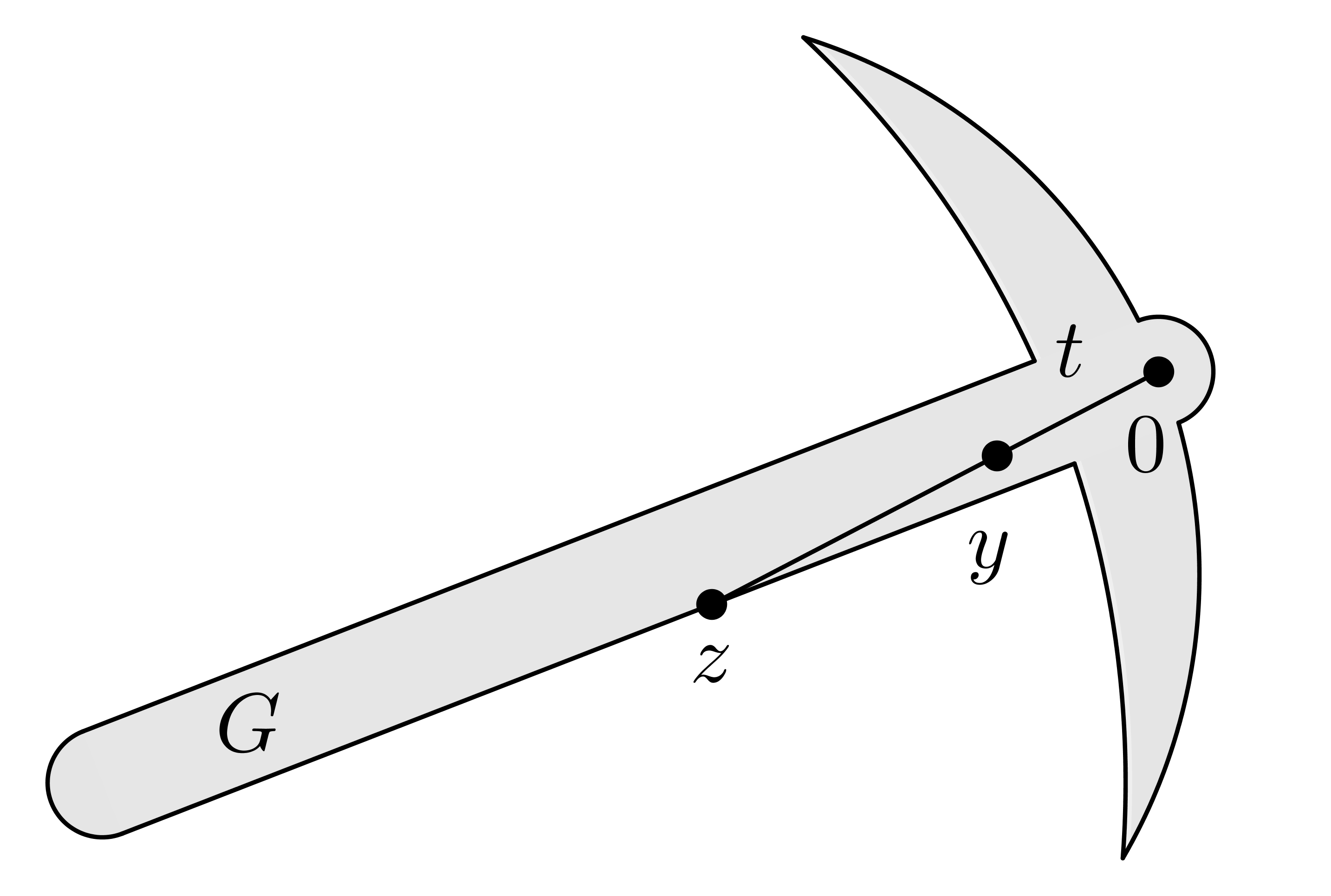
In this article we are interested in the growth of hyperbolic type distances in proper subdomains G⊊ℝnG\subsetneq{\mathbb{R}^{n}}. We consider the growth along a Euclidean line segment from z′∈Gz^{\prime}\in G to z∈∂Gz\in\partial G. By a linear transformation we may assume that z′=0z^{\prime}=0. To ensure that the line segment [z′,z)[z^{\prime},z) is in GG we restrict our study to starlike domains, which means that for every y∈Gy\in G the Euclidean line segment [x,y][x,y] is contained in GG.

Let G⊂ℝnG\subset{\mathbb{R}^{n}} be a starlike domain and z∈∂Gz\in\partial G. Let y∈[0,z)y\in[0,z) and denote t=|y|t=|y|. We study the behaviour of the function

fm​(t)=m⁡(0,y)=m⁡(0,t​z/|z|),f_{m}(t)=m(0,y)=m(0,tz/|z|), (1.1)
Refer to caption
Figure 1: Starlike domain GG and the function fm​(t)=m⁡(0,t​z/|z|)=m⁡(0,y)f_{m}(t)=m(0,tz/|z|)=m(0,y).

where mm is a hyperbolic type distance, see Figure 1. Note that now fmf_{m} is a continuous mapping from [0,|z|)[0,|z|) to [0,∞)[0,\infty). To study this function we start of with an easier one

g⁡(t)=dG​(y)=d⁡(y,∂G)=d⁡(t​z/|z|,∂G).g(t)=d_{G}(y)=d(y,\partial G)=d(tz/|z|,\partial G). (1.2)

All the results of our study are true in a more general setting as long as the line segment [0,z)[0,z) is contained in the domain. However, we consider starlike domains as then this condition is clearly fulfilled.

Our main result is the following Schwarz lemma type theorem. For definition of the distances see the section named after the distance.

Theorem 1.3.

Let G⊊ℝnG\subsetneq{\mathbb{R}^{n}} be a domain with 0∈G0\in G and fm​(t)f_{m}(t) be the function defined in (1.1) for any z∈∂Gz\in\partial G. For m∈{j,k,σ~,c}m\in\{j,k,\widetilde{\sigma},c\}

fm′​(0)=1dG​(0)f_{m}^{\prime}(0)=\frac{1}{d_{G}(0)}

and for m∈{α,δ}m\in\{\alpha,\delta\}

1dG​(0)≤fm′​(0)≤2dG​(0),\frac{1}{d_{G}(0)}\leq f_{m}^{\prime}(0)\leq\frac{2}{d_{G}(0)},

where the upper and lower bounds are best possible, and

0≤fτ~′​(0)≤1dG​(0).0\leq f_{\widetilde{\tau}}^{\prime}(0)\leq\frac{1}{d_{G}(0)}.

2 Preliminaries and the hyperbolic distance, ρG\rho_{G}

In this section we introduce notation and consider examples of the hyperbolic distance in the upper half space and a ball.

For a,b∈ℝna,b\in{\mathbb{R}^{n}} we denote the closed Euclidean line segment between the points by [a,b]={c∈ℝn:c=x+t(y−x), 0≤t≤1}[a,b]=\{c\in{\mathbb{R}^{n}}\colon c=x+t(y-x),\,0\leq t\leq 1\}. We also use notation (a,b)(a,b), [a,b)[a,b) and (a,b](a,b] for open and half-closed line segments in ℝn{\mathbb{R}^{n}}. We denote the smallest angle between line segments [a,b][a,b] and [b,c][b,c] by ∡⁡(a,b,c)\measuredangle(a,b,c).

We denote Euclidean balls and spheres with centre x∈ℝnx\in{\mathbb{R}^{n}} and radius r>0r>0, respectively, by Bn​(x,r)B^{n}(x,r) and Sn−1​(x,r)S^{n-1}(x,r). A domain G⊊ℝnG\subsetneq{\mathbb{R}^{n}}, 0∈G0\in G, is said to be starlike, if it is strictly starlike with respect to 00: for every z∈∂Gz\in\partial G the line segment [0,z)[0,z) is contained in GG. We say that distance function mGm_{G} in G⊊∈ℝnG\subsetneq\in{\mathbb{R}^{n}} is hyperbolic type, if m𝔹n≈ρ𝔹nm_{\mathbb{B}^{n}}\approx\rho_{\mathbb{B}^{n}}, where ρ𝔹n\rho_{\mathbb{B}^{n}} is the hyperbolic distance in the unit ball defined in (2.2).

Let b<0b<0. The hyperbolic distance for all u,w∈ℍbn={a∈ℝn:an>b}u,w\in{\mathbb{H}^{n}_{b}}=\{a\in{\mathbb{R}^{n}}\colon a_{n}>b\} is defined as

fρℍbn​(t)=ρℍbn​(u,w)=arc cosh ​(1+|u−w|22​|un−b|​|wn−b|).f_{\rho_{\mathbb{H}^{n}_{b}}}(t)=\rho_{\mathbb{H}^{n}_{b}}(u,w)=\textrm{arc\,cosh\,}\left(1+\frac{|u-w|^{2}}{2|u_{n}-b||w_{n}-b|}\right).

Note that we use shifted version of the upper half space, as the usual upper half space ℍn={a∈ℝn:an>0}{\mathbb{H}^{n}}=\{a\in{\mathbb{R}^{n}}\colon a_{n}>0\} does not contain the origin.

Example 2.1.

Let z=(0,0,…,0,b)∈∂Gz=(0,0,\dots,0,b)\in\partial G and y∈[0,z)y\in[0,z) with |y|=t|y|=t. We show that in this case fρℍbn′​(0)=1/dℍbn​(0)f_{\rho_{\mathbb{H}^{n}_{b}}}^{\prime}(0)=1/d_{\mathbb{H}^{n}_{b}}(0).

Now for t∈(0,dℍbn​(0))t\in(0,d_{\mathbb{H}^{n}_{b}}(0)) we have

fρℍbn​(t)=ρℍbn​(0,y)\displaystyle f_{\rho_{\mathbb{H}^{n}_{b}}}(t)=\rho_{\mathbb{H}^{n}_{b}}(0,y) =\displaystyle= arc cosh ​(1+|y|22​|b|​|yn−b|)\displaystyle\textrm{arc\,cosh\,}\left(1+\frac{|y|^{2}}{2|b||y_{n}-b|}\right)
=\displaystyle= arc cosh ​(1+t22​dℍbn​(0)​(dℍbn​(0)−t))\displaystyle\textrm{arc\,cosh\,}\left(1+\frac{t^{2}}{2d_{\mathbb{H}^{n}_{b}}(0)(d_{\mathbb{H}^{n}_{b}}(0)-t)}\right)

and by differentiation we obtain

fρℍbn′​(t)=1dℍbn​(0)−t.f_{\rho_{\mathbb{H}^{n}_{b}}}^{\prime}(t)=\frac{1}{d_{\mathbb{H}^{n}_{b}}(0)-t}.

We consider fρℍbn′​(0)f_{\rho_{\mathbb{H}^{n}_{b}}}^{\prime}(0) by taking the limit fρℍbn′​(t)→1/dℍbn​(0)f_{\rho_{\mathbb{H}^{n}_{b}}}^{\prime}(t)\to 1/d_{\mathbb{H}^{n}_{b}}(0) as t→0t\to 0. △\triangle

Let B=Bn​(x,r)B=B^{n}(x,r) be a ball with x∈ℝnx\in{\mathbb{R}^{n}} and r>0r>0. For u,w∈Bu,w\in B the hyperbolic distance is defined by

ρB​(u,w)=arc sinh ​|u−w|/r1−|u|2/r2​1−|w|2/r2.\rho_{B}(u,w)=\textrm{arc\,sinh\,}\frac{|u-w|/r}{\sqrt{1-|u|^{2}/r^{2}}\sqrt{1-|w|^{2}/r^{2}}}. (2.2)
Example 2.3.

Let z∈∂Bz\in\partial B and x∈[0,z)x\in[0,z). We show that in this case fρB′​(0)=1/dB​(0)f_{\rho_{B}}^{\prime}(0)=1/d_{B}(0).

Now for t∈(0,dB​(0))t\in(0,d_{B}(0))

fρB​(t)=ρB​(0,y)\displaystyle f_{\rho_{B}}(t)=\rho_{B}(0,y) =\displaystyle= arc sinh ​|y|/r1−|y|2/r2\displaystyle\textrm{arc\,sinh\,}\frac{|y|/r}{\sqrt{1-|y|^{2}/r^{2}}}
=\displaystyle= arc sinh ​t/dB​(0)1−t2/dB​(0)2\displaystyle\textrm{arc\,sinh\,}\frac{t/d_{B}(0)}{\sqrt{1-t^{2}/d_{B}(0)^{2}}}

and fρB′​(t)=dB​(0)/(dB​(0)2−t2)f_{\rho_{B}}^{\prime}(t)=d_{B}(0)/(d_{B}(0)^{2}-t^{2}). Taking the limit we obtain fρB′​(t)→1/dB​(0)f_{\rho_{B}}^{\prime}(t)\to 1/d_{B}(0) as t→0t\to 0. △\triangle

Examples 2.1 and 2.3 suggest that for hyperbolic type distances fm′​(0)=a/dG​(0)f_{m}^{\prime}(0)=a/d_{G}(0) could hold for a≥0a\geq 0 or perhaps even for a=1a=1. It turns out that this conjecture is not true in general. However, based on our study in this article, it seems that the following is true

Conjecture 2.4.

For a hyperbolic type distance mm there exists constants a≥0a\geq 0 and b≥1b\geq 1 such that

adG​(0)≤fm′​(0)≤bdG​(0).\frac{a}{d_{G}(0)}\leq f_{m}^{\prime}(0)\leq\frac{b}{d_{G}(0)}.

3 Distance to the boundary function, dGd_{G}

In this section we study the problem for the distance to the boundary function g⁡(t)g(t) formulated in (1.2). Let us begin our study with few simple planar examples, which are easy to reconstruct in higher dimensions.

Example 3.1.

We consider starlike domain

G=ℝ2∖Rx,Rx={w=(w1,w2)∈R2:w1≥x1,w2≥x2},G=\mathbb{R}^{2}\setminus R_{x},\hskip 10.00002ptR_{x}=\{w=(w_{1},w_{2})\in R^{2}\colon w_{1}\geq x_{1},\,w_{2}\geq x_{2}\},

where x=(x1,x2)∈ℝ2x=(x_{1},x_{2})\in\mathbb{R}^{2} with x1,x2>0x_{1},x_{2}>0. For a given z=z⁡(α)z=z(\alpha) we derive a formula for g⁡(t)g(t) and show that g⁡(t)=(|z|−t)​sin⁡αg(t)=(|z|-t)\sin\alpha and thus linear for large values of tt. We choose z=(x1,y2)z=(x_{1},y_{2}) for z2≥x2z_{2}\geq x_{2} and note that z∈∂Gz\in\partial G.

Refer to caption
Refer to caption
Figure 2: The domains GG of Examples 3.1 (on left) and 3.2 (on right).

When tt is small, then yy is close to 00 and g⁡(t)=|y−x|g(t)=|y-x|. To be more explicit we can write

g⁡(t)=dG​(y)=|y−x|=|a−x|2+|a−y|2,if ​t≤|a|,g(t)=d_{G}(y)=|y-x|=\sqrt{|a-x|^{2}+|a-y|^{2}},\hskip 10.00002pt\textrm{if }t\leq|a|,

where aa is the point in [0,z][0,z], with a2=x2a_{2}=x_{2}, see Figure 2.

If tt is faraway from 00, the we have

g⁡(t)=d⁡(y,l)=|y−z|​sin⁡α,if ​t≥|a|,g(t)=d(y,l)=|y-z|\sin\alpha,\hskip 10.00002pt\textrm{if }t\geq|a|,

where l={(x1,t):t∈ℝ}l=\{(x_{1},t)\colon t\in\mathbb{R}\} and α=∡⁡(y,z,x)\alpha=\measuredangle(y,z,x).

Next we want to express our function g⁡(t)g(t) in terms of tt and points xx and zz. We easily obtain |y−z|=|z|−t|y-z|=|z|-t, |a−z|=|x−z|​cos⁡α|a-z|=|x-z|\cos\alpha, |a−x|=|x−z|​sin⁡α|a-x|=|x-z|\sin\alpha, |a−y|=|z|−t−|a−z||a-y|=|z|-t-|a-z| and

|a|=|z|−|a−z|=|z|−|x−z|cos⁡α.|a|=|z|-|a-z|=|z|-|x-z|\cos\alpha.

Putting all together gives

g⁡(t)={t2−2​t​(|z|−|a−z|)+|z|(|z|−2​|a−z|)+|x−z|2,if ​t≤|a|,(|z|−t)​sin⁡α,if ​t>|a|,g(t)=\left\{\begin{array}[]{ll}\sqrt{t^{2}-2t(|z|-|a-z|)+|z|(|z|-2|a-z|)+|x-z|^{2}},&\textrm{if }t\leq|a|,\\ (|z|-t)\sin\alpha,&\textrm{if }t>|a|,\end{array}\right.

and here |a−z|=|x−z|​cos⁡α|a-z|=|x-z|\cos\alpha. △\triangle

Example 3.2.

Let us consider starlike domain G=𝔹2∖(B2​(1+i,1)𝐶𝐿𝑂𝑆𝐸¯∪B2​(−1+i,1)¯∪B2​(−1−i,1)¯∪𝑂𝑃𝐸𝑁B2​(1−i,1))¯G=\mathbb{B}^{2}\setminus\overline{(B^{2}(1+i,1)}\cup\overline{B^{2}(-1+i,1)}\cup\overline{B^{2}(-1-i,1)}\cup\overline{B^{2}(1-i,1))} and z=1∈∂Gz=1\in\partial G, see Figure 2.

For y∈[0,z)y\in[0,z) and t=|y|∈[0,1)t=|y|\in[0,1) we have

g⁡(t)=dG​(y)=|y−(1+i)|−1=t2−2​t+2−1.g(t)=d_{G}(y)=|y-(1+i)|-1=\sqrt{t^{2}-2t+2}-1.

Now

g′​(t)=t−1t2−2​t+2g^{\prime}(t)=\frac{t-1}{\sqrt{t^{2}-2t+2}}

implying g′​(t)→0g^{\prime}(t)\to 0 as t→1t\to 1. △\triangle

Example 3.3.

In Example 3.2 we could place the circular arc with any decreasing function: First define a decreasing function h:[0,1]→[0,1]h\colon[0,1]\to[0,1] with h⁡(0)=1h(0)=1 and h⁡(1)=0h(1)=0. Then reflect the function across the real axis and then reflect both function across the imaginary axis.

For p∈{1,2,…}p\in\{1,2,\dots\} we can define polynomial function h⁡(t)=(1−t)ph(t)=(1-t)^{p} to obtain a domain GG. Now for z=1∈∂Gz=1\in\partial G we have

g⁡(t)=(1−t)2​p+(1−t)4​p−2.g(t)=\sqrt{(1-t)^{2p}+(1-t)^{4p-2}}.

and since (1−t)2​p+(1−t)4​p−2≥(1−t)2​p=(1−t)p\sqrt{(1-t)^{2p}+(1-t)^{4p-2}}\geq\sqrt{(1-t)^{2p}}=(1-t)^{p} we obtain

g′​(t)\displaystyle g^{\prime}(t) =\displaystyle= −2​p​(1−t)2​p−1−(4​p−2)​(1−t)4​p−32​(1−t)2​p+(1−t)4​p−2\displaystyle\frac{-2p(1-t)^{2p-1}-(4p-2)(1-t)^{4p-3}}{2\sqrt{(1-t)^{2p}+(1-t)^{4p-2}}}
≤\displaystyle\leq −2​p​(1−t)2​p−1−(4​p−2)​(1−t)4​p−32​(1−t)p\displaystyle\frac{-2p(1-t)^{2p-1}-(4p-2)(1-t)^{4p-3}}{2(1-t)^{p}}
=\displaystyle= −p​(1−t)p−1−(2​p−1)​(1−t)3​p−3→0\displaystyle-p(1-t)^{p-1}-(2p-1)(1-t)^{3p-3}\to 0

as t→1t\to 1. △\triangle

Let us then consider general case G⊊ℝnG\subsetneq{\mathbb{R}^{n}}. How quickly and how slowly g⁡(t)g(t) can decrease for large values of tt? How quickly and how slowly g⁡(t)g(t) can increase for tt close to 00? Before considering the bounds for g⁡(t)g(t), we introduce angular domain.

For x,y∈ℝnx,y\in{\mathbb{R}^{n}} and α∈(0,π)\alpha\in(0,\pi) we define

Sα,x,y={z∈ℝn:∡⁡(y,x,z)≤α}.S_{\alpha,x,y}=\{z\in{\mathbb{R}^{n}}\colon\measuredangle(y,x,z)\leq\alpha\}.

If tt is close to 00, then the slowest growth for g⁡(t)g(t) occurs in the following case:

G1=ℝn∖(Sπ/4,−x,−2​x∪Sπ/4,3​x,4​x)G_{1}={\mathbb{R}^{n}}\setminus(S_{\pi/4,-x,-2x}\cup S_{\pi/4,3x,4x}) (3.4)

for some x∈ℝn∖{0}x\in{\mathbb{R}^{n}}\setminus\{0\} and z=3​xz=3x, see Figure 3. Now for t∈[0,|x|]t\in[0,|x|], we have

g⁡(t)=dG​(0)+t=|x|+t.g(t)=d_{G}(0)+t=|x|+t. (3.5)
Refer to caption
Figure 3: The domain G1=ℝn∖(Sπ/4,−x,−2​x∪Sπ/4,3​x,4​x)G_{1}={\mathbb{R}^{n}}\setminus(S_{\pi/4,-x,-2x}\cup S_{\pi/4,3x,4x}) defined in (3.4) for the extremal case, when tt is close to 00.

If tt is faraway from the boundary, then the slowest growth occurs in the case

G2=ℝn∖Sπ/4,x,2​xG_{2}={\mathbb{R}^{n}}\setminus S_{\pi/4,x,2x} (3.6)

for any x∈ℝn∖{0}x\in{\mathbb{R}^{n}}\setminus\{0\} and z=xz=x. Now

g⁡(t)=dG​(0)−t=|x|−tg(t)=d_{G}(0)-t=|x|-t

for t∈[0,|z|)t\in[0,|z|).

As we will later see, it turns out that the domains G1G_{1} and G2G_{2} defined respectively in (3.4) and (3.6) can be used as extremal domains for many hyperbolic type distances. Note that if GG was not starlike, we could use G1′=ℝn∖{−x,3​x}G_{1}^{\prime}={\mathbb{R}^{n}}\setminus\{-x,3x\} and G2′=ℝn∖{x}G_{2}^{\prime}={\mathbb{R}^{n}}\setminus\{x\} instead of G1G_{1} and G2G_{2}.

Next we consider how quickly g⁡(t)g(t) can decrease. Close to the origin the fastest decrement occurs in the domain G=Bn​(0,dG​(0))G=B^{n}(0,d_{G}(0)) and it is

g⁡(t)=dG​(0)−tg(t)=d_{G}(0)-t (3.7)

for t∈[0,dG​(0))t\in[0,d_{G}(0)).

Faraway from the origin the decrement can made arbitrarily slow as can be observed from Examples 3.1, 3.2 and 3.3. We have arrived to the following theorem:

Theorem 3.8.

For any starlike domain GG and point z∈∂Gz\in\partial G we have

g′​(t)≤1,for ​t∈[0,|z|).g^{\prime}(t)\leq 1,\hskip 10.00002pt\textrm{for }t\in[0,|z|).

Moreover,

−1≤g′​(0)≤1and−1≤limt→|z|g′​(t)≤0.-1\leq g^{\prime}(0)\leq 1\hskip 10.00002pt\textrm{and}\hskip 10.00002pt-1\leq\lim_{t\to|z|}g^{\prime}(t)\leq 0.

4 Distance ratio distance, jGj_{G}

In this section we estimate fj​(t)f_{j}(t) for the distance ratio distance jGj_{G}, which is defined in any open subset G⊊ℝnG\subsetneq{\mathbb{R}^{n}} for points u,w∈Gu,w\in G by

jG​(u,w)=log⁡(1+|u−w|min⁡{dG​(u),dG​(w)}).j_{G}(u,w)=\log\left(1+\frac{|u-w|}{\min\{d_{G}(u),d_{G}(w)\}}\right).

The distance ratio distance was introduced by Vuorinen in the 1980’s [17] and in a slightly different form by Gehring and Osgood [4].

For fj​(t)f_{j}(t) we can use the same domains as for g⁡(t)g(t) to consider the extremal cases. Note that the following result is true also in non starlike domains.

Theorem 4.1.

Let G⊊ℝnG\subsetneq{\mathbb{R}^{n}} be a starlike domain and z∈∂Gz\in\partial G. For the distance ratio distance jGj_{G} we have fj′​(0)=1/dG​(0)f_{j}^{\prime}(0)=1/d_{G}(0),

fj​(t)≥log⁡(1+tdG​(0))for all ​t∈[0,|z|),f_{j}(t)\geq\log\left(1+\frac{t}{d_{G}(0)}\right)\hskip 10.00002pt\textrm{for all }t\in[0,|z|),

and

fj​(t)≤log⁡(dG​(0)OPENdG​(0)−t))for all ​t∈[0,dG​(0)).f_{j}(t)\leq\log\left(\frac{d_{G}(0)}{d_{G}(0)-t)}\right)\hskip 10.00002pt\textrm{for all }t\in[0,d_{G}(0)).
Proof.

Let us first consider lower bound for fj​(0)f_{j}(0). We denote a closest boundary x∈∂Gx\in\partial G with dG​(0)=|0−x|d_{G}(0)=|0-x| and z∈∂Gz\in\partial G. Now y∈[0,|z|)y\in[0,|z|) with |y|=t|y|=t we have

fj​(t)\displaystyle f_{j}(t) =\displaystyle= jG​(0,y)=log⁡(1+|y|min⁡{dG​(0),dG​(y)})\displaystyle j_{G}(0,y)=\log\left(1+\frac{|y|}{\min\{d_{G}(0),d_{G}(y)\}}\right)
≥\displaystyle\geq log⁡(1+tdG​(0)):=l⁡(t).\displaystyle\log\left(1+\frac{t}{d_{G}(0)}\right):=l(t).

This is obtained for example as in (3.5) in the domain G1=ℝn∖(Sπ/4,−x,−2​x∪Sπ/4,3​x,4​x)G_{1}={\mathbb{R}^{n}}\setminus(S_{\pi/4,-x,-2x}\cup S_{\pi/4,3x,4x}) for some x∈ℝn∖{0}x\in{\mathbb{R}^{n}}\setminus\{0\} and z=3​xz=3x.

Let us then consider upper bound for fj​(0)f_{j}(0). Now as dG​(0)d_{G}(0) is a constant we may assume dG​(y)≤dG​(0)d_{G}(y)\leq d_{G}(0) and obtain by (3.7)

fj​(t)\displaystyle f_{j}(t) =\displaystyle= log⁡(1+|y|min⁡{dG​(0),dG​(y)})≤log⁡(1+tdG​(y))\displaystyle\log\left(1+\frac{|y|}{\min\{d_{G}(0),d_{G}(y)\}}\right)\leq\log\left(1+\frac{t}{d_{G}(y)}\right)
=\displaystyle= log⁡(1+tdG​(0)−t)=log⁡(dG​(0)OPENdG​(0)−t))=:u⁡(t).\displaystyle\log\left(1+\frac{t}{d_{G}(0)-t}\right)=\log\left(\frac{d_{G}(0)}{d_{G}(0)-t)}\right)=:u(t).

This situation is obtained in the domain G′=Bn​(0,dG​(0))G^{\prime}=B^{n}(0,d_{G}(0)), because for any GG we have G′⊂GG^{\prime}\subset G.

The upper and lower bounds of fj​(t)f_{j}(t) give us

limt→0l′​(t)=limt→01dG​(0)+t≤fj′​(0)≤limt→0u′​(t)=limt→01dG​(0)−t\lim_{t\to 0}l^{\prime}(t)=\lim_{t\to 0}\frac{1}{d_{G}(0)+t}\leq f_{j}^{\prime}(0)\leq\lim_{t\to 0}u^{\prime}(t)=\lim_{t\to 0}\frac{1}{d_{G}(0)-t}

which yields fj′​(0)=1/dG​(0)f_{j}^{\prime}(0)=1/d_{G}(0). ∎

Note that the lower bound for fj​(t)f_{j}(t) in Theorem 4.1 works for all tt whereas the upper bound holds only close to the origin. As a matter of fact, by Theorem 3.8, the function g′​(t)g^{\prime}(t) can be arbitrarily close to zero near the boundary and therefore we cannot find an upper bound for fj​(t)f_{j}(t) in this case.

5 Quasihyperbolic distance, kGk_{G}

Next we consider the quasihyperbolic distance. Let G⊊ℝnG\subsetneq{\mathbb{R}^{n}} be a domain. We define the quasihyperbolic length of a curve γ⊂G\gamma\subset G by

ℓk​(γ)=∫γ|d​u|dG​(u).\ell_{k}(\gamma)=\int_{\gamma}\frac{|du|}{d_{G}(u)}.

For u,w∈Gu,w\in G the quasihyperbolic distance between uu and ww is define by

kG​(u,w)=infγu​wℓ⁡(γu​w),k_{G}(u,w)=\inf_{\gamma_{uw}}\ell(\gamma_{uw}),

where the infimum is taken over all rectifiable curves γu​w\gamma_{uw} joining uu and ww in GG. The quasihyperbolic distance was introduced in the 1970’s by Gehring and Palka [4].

Theorem 5.1.

Let G⊊ℝnG\subsetneq{\mathbb{R}^{n}} be a starlike domain and z∈∂Gz\in\partial G. For the quasihyperbolic distance kGk_{G} we have fk′​(0)=1/dG​(0)f_{k}^{\prime}(0)=1/d_{G}(0),

fk​(t)≥log⁡(1+tdG​(0))for all ​t∈[0,|z|),f_{k}(t)\geq\log\left(1+\frac{t}{d_{G}(0)}\right)\hskip 10.00002pt\textrm{for all }t\in[0,|z|),

and

fk​(t)≤log⁡(dG​(0)OPENdG​(0)−t))for all ​t∈[0,dG​(0)).f_{k}(t)\leq\log\left(\frac{d_{G}(0)}{d_{G}(0)-t)}\right)\hskip 10.00002pt\textrm{for all }t\in[0,d_{G}(0)).
Proof.

We start by finding a lower bound for fk​(t)f_{k}(t). Let z∈∂Gz\in\partial G and y∈[0,z)y\in[0,z). For t=|z|t=|z| we estimate

f⁡(t)\displaystyle f(t) =\displaystyle= kG​(0,y)=∫γ|d​u|dG​(u)≥∫[0,y]|d​u|dG​(0)+u=∫0td​udG​(0)+u\displaystyle k_{G}(0,y)=\int_{\gamma}\frac{|du|}{d_{G}(u)}\geq\int_{[0,y]}\frac{|du|}{d_{G}(0)+u}=\int_{0}^{t}\frac{du}{d_{G}(0)+u}
=\displaystyle= log⁡(dG​(0)+t)−log⁡dG​(0)=log⁡(1+tdG​(0)).\displaystyle\log(d_{G}(0)+t)-\log d_{G}(0)=\log\left(1+\frac{t}{d_{G}(0)}\right).

For G′=Bn​(0,dG​(0))G^{\prime}=B^{n}(0,d_{G}(0)) and y∈[0,dG​(0))y\in[0,d_{G}(0)) clearly dG′​(0)=dG​(0)d_{G^{\prime}}(0)=d_{G}(0) and we obtain

f⁡(t)\displaystyle f(t) =\displaystyle= kG​(0,t​z/|z|)≤kG′​(0,t​z/|z|)=∫0td​sdG​(0)−s\displaystyle k_{G}(0,tz/|z|)\leq k_{G^{\prime}}(0,tz/|z|)=\int_{0}^{t}\frac{ds}{d_{G}(0)-s}
=\displaystyle= −log⁡(dG​(0)−t)+log⁡dG​(0)=log⁡dG​(0)dG​(0)−t.\displaystyle-\log(d_{G}(0)-t)+\log d_{G}(0)=\log\frac{d_{G}(0)}{d_{G}(0)-t}.

The lower and the upper bounds of fk​(t)f_{k}(t) are equal to the corresponding bounds for fj​(t)f_{j}(t) and the expression for fk′​(0)f_{k}^{\prime}(0) follows as in the proof of Theorem 4.1. ∎

Exactly same observation for fk​(t)f_{k}(t) near the boundary can be made that we made for the distance ratio distance. Theorem 5.1 gives a lower bound and an upper bound can not be obtained.

6 Triangular ratio distance, sGs_{G} (σG\sigma_{G})

For a domain G⊊ℝnG\subsetneq{\mathbb{R}^{n}} and points u,w∈Gu,w\in G we define the triangular ratio distance by

sG​(u,w)=supq∈∂G|u−w||u−q|+|q−w|.s_{G}(u,w)=\sup_{q\in\partial G}\frac{|u-w|}{|u-q|+|q-w|}.

Geometrically the supremum is attained at a point qq such that it is either on line segment [u,w][u,w] or if this is not possible, then qq is on the largest ellipsoid with focii uu and ww contained in GG. The triangular ratio distance was introduced by Hästö in the 2000’s [7]. Since sG∈[0,1]s_{G}\in[0,1] we observe that sGs_{G} is not hyperbolic type. For u,w∈Gu,w\in G we define

σG​(u,w)=tan⁡π​sG​(u,w)2\sigma_{G}(u,w)=\tan\frac{\pi s_{G}(u,w)}{2}

to obtain a hyperbolic type distance.

As in the case of the distance to the boundary function and the distance ratio distance we can use the same extremal domains. The domain G1=ℝn∖(Sπ/4,−x,−2​x∪Sπ/4,3​x,4​x)G_{1}={\mathbb{R}^{n}}\setminus(S_{\pi/4,-x,-2x}\cup S_{\pi/4,3x,4x}) for some x∈ℝn∖{0}x\in{\mathbb{R}^{n}}\setminus\{0\} and z=3​xz=3x gives lower bound

fs​(t)≥tdG​(0)+(dG​(0)+t)=t2​dG​(0)+tf_{s}(t)\geq\frac{t}{d_{G}(0)+(d_{G}(0)+t)}=\frac{t}{2d_{G}(0)+t} (6.1)

for t∈[0,|z|)t\in[0,|z|).

The domain G2=ℝn∖Sπ/4,x,2​xG_{2}={\mathbb{R}^{n}}\setminus S_{\pi/4,x,2x} for any x∈ℝn∖{0}x\in{\mathbb{R}^{n}}\setminus\{0\} and z=xz=x gives upper bound

fs​(t)≤tdG​(y)+(dG​(y)−t)=t2​dG​(0)−tf_{s}(t)\leq\frac{t}{d_{G}(y)+(d_{G}(y)-t)}=\frac{t}{2d_{G}(0)-t} (6.2)

for t∈[0,d⁡(0))t\in[0,d(0)).

Combining these estimates we obtain:

Theorem 6.3.

Let G⊊ℝnG\subsetneq{\mathbb{R}^{n}} be a starlike domain and z∈∂Gz\in\partial G. Then

fσ​(t)≥tan⁡π​t4​dG​(0)+2​tf_{\sigma}(t)\geq\tan\frac{\pi t}{4d_{G}(0)+2t}

for t∈[0,|z|)t\in[0,|z|) and

fσ​(t)≤tan⁡π​t4​dG​(0)−2​tf_{\sigma}(t)\leq\tan\frac{\pi t}{4d_{G}(0)-2t}

for t∈[0,d⁡(0))t\in[0,d(0)). Moreover, fσ′​(0)=π/(4​dG​(0))f_{\sigma}^{\prime}(0)=\pi/(4d_{G}(0)).

Proof.

The bounds for fσ​(t)f_{\sigma}(t) follow from (6.1) and (6.2). By differentiation we obtain

∂∂t​tan⁡π​t4​dG​(0)±2​t=π​dG​(0)+4​π​dG​(0)​tan2⁡π​t4​dG​(0)±2​t4​dG​(0)2±4​dG​(0)​t+t2\frac{\partial}{\partial t}\tan\frac{\pi t}{4d_{G}(0)\pm 2t}=\frac{\pi d_{G}(0)+4\pi d_{G}(0)\tan^{2}\displaystyle\frac{\pi t}{4d_{G}(0)\pm 2t}}{4d_{G}(0)^{2}\pm 4d_{G}(0)t+t^{2}}

and thus fσ​´​(0)=π/(4​dG​(0))f_{\sigma}\textasciiacute(0)=\pi/(4d_{G}(0)). ∎

Remark 6.4.

Theorem 6.3 suggests that an alternative way to define a hyperbolic type distance by using the triangular ratio distance, could be σ~G​(u,w)=4π​σG​(u,w)\widetilde{\sigma}_{G}(u,w)=\tfrac{4}{\pi}\sigma_{G}(u,w). For this distance function fσ~′​(0)=1/dG​(0)f_{\widetilde{\sigma}}^{\prime}(0)=1/d_{G}(0).

7 Cassinian distance, cGc_{G}

For a domain G⊊ℝnG\subsetneq{\mathbb{R}^{n}} and points u,w∈Gu,w\in G we define the Cassinian distance by

cG​(u,w)=supq∈∂G|u−w||u−q|​|q−w|.c_{G}(u,w)=\sup_{q\in\partial G}\frac{|u-w|}{|u-q||q-w|}.

The Cassinian distance was introduced by Ibragimov in the 2000’s [8]. In the plane case the supremum is attained at a point qq that is on the largest Cassinian oval with focii uu and ww contained in GG.

Theorem 7.1.

Let G⊊ℝnG\subsetneq{\mathbb{R}^{n}} be a starlike domain and z∈∂Gz\in\partial G. Then

fc​(t)≥tdG​(0)​(dG​(0)+t)f_{c}(t)\geq\frac{t}{d_{G}(0)(d_{G}(0)+t)}

for t∈[0,|z|)t\in[0,|z|) and

fc​(t)≤tdG​(0)​(dG​(0)−t)f_{c}(t)\leq\frac{t}{d_{G}(0)(d_{G}(0)-t)}

for t∈[0,d⁡(0))t\in[0,d(0)). Moreover, fc′​(0)=1/dG​(0)f_{c}^{\prime}(0)=1/d_{G}(0).

Proof.

The domain G1=ℝn∖(Sπ/4,−x,−2​x∪Sπ/4,3​x,4​x)G_{1}={\mathbb{R}^{n}}\setminus(S_{\pi/4,-x,-2x}\cup S_{\pi/4,3x,4x}) for some x∈ℝn∖{0}x\in{\mathbb{R}^{n}}\setminus\{0\} and z=3​xz=3x gives lower bound

fc​(t)≥tdG​(0)​(dG​(0)+t)f_{c}(t)\geq\frac{t}{d_{G}(0)(d_{G}(0)+t)}

for t∈[0,|z|)t\in[0,|z|).

The domain G2=ℝn∖Sπ/4,x,2​xG_{2}={\mathbb{R}^{n}}\setminus S_{\pi/4,x,2x} for any x∈ℝn∖{0}x\in{\mathbb{R}^{n}}\setminus\{0\} and z=xz=x gives upper bound

fc​(t)≤tdG​(y)​(dG​(y)+t)=tdG​(0)​(dG​(0)−t)f_{c}(t)\leq\frac{t}{d_{G}(y)(d_{G}(y)+t)}=\frac{t}{d_{G}(0)(d_{G}(0)-t)}

for t∈[0,d⁡(0))t\in[0,d(0)).

Differentiation gives

∂∂t​tdG​(0)​(dG​(0)±t)=dG​(0)dG​(0)2±2​dG​(0)​t+t2\frac{\partial}{\partial t}\frac{t}{d_{G}(0)(d_{G}(0)\pm t)}=\frac{d_{G}(0)}{d_{G}(0)^{2}\pm 2d_{G}(0)t+t^{2}}

and clearly fc′​(0)=1/dG​(0)f_{c}^{\prime}(0)=1/d_{G}(0). ∎

8 Apollonian distance, αG\alpha_{G}

Let G⊂ℝn¯G\subset\overline{{\mathbb{R}^{n}}} be a domain such that ∂G\partial G is not contained in a sphere in ℝn¯\overline{{\mathbb{R}^{n}}}. Then for u,w∈Gu,w\in G we define the Apollonian distance [3, Theorem 1.1] by

αG​(u,w)=supa,b∈∂Glog⁡|a−w|​|b−u||a−u|​|b−w|.\alpha_{G}(u,w)=\sup_{a,b\in\partial G}\log\frac{|a-w||b-u|}{|a-u||b-w|}.

The Apollonian distance was introduced by Barbilian in the 1930’s [2] and reintroduced by Beardon in the 1990’s in connection with the hyperbolic metric [3]. It is worth pointing out that we can write

αG​(u,w)=supa∈∂Glog⁡|a−w||a−u|+supb∈∂Glog⁡|b−u||b−w|\alpha_{G}(u,w)=\sup_{a\in\partial G}\log\frac{|a-w|}{|a-u|}+\sup_{b\in\partial G}\log\frac{|b-u|}{|b-w|} (8.1)

and in the case n=2n=2 each quotient defines an Apollonian circle. Taking the supremum means that we take the largest possible Apollonian circles in G¯\overline{G}.

Lemma 8.2.

Let u∈ℝnu\in{\mathbb{R}^{n}}, r>0r>0 and w∈Bn​(u,r)w\in B^{n}(u,r). Denote S=Sn−1​(u,r)S=S^{n-1}(u,r). Then

supa∈S|w−a||u−a|=r+|u−w|r,supa∈S|u−a||w−a|=rr−|u−w|,\sup_{a\in S}\frac{|w-a|}{|u-a|}=\frac{r+|u-w|}{r},\hskip 10.00002pt\sup_{a\in S}\frac{|u-a|}{|w-a|}=\frac{r}{r-|u-w|},

and for r′>rr^{\prime}>r and S′=Sn−1​(u,r′)S^{\prime}=S^{n-1}(u,r^{\prime})

supa∈S′|w−a||u−a|≤supa∈S|w−a||u−a|,supa∈S′|u−a||w−a|≤supa∈S|u−a||w−a|.\sup_{a\in S^{\prime}}\frac{|w-a|}{|u-a|}\leq\sup_{a\in S}\frac{|w-a|}{|u-a|},\hskip 10.00002pt\sup_{a\in S^{\prime}}\frac{|u-a|}{|w-a|}\leq\sup_{a\in S}\frac{|u-a|}{|w-a|}.
Proof.

To simplify notation we may assume that u=0u=0 and w=β​e1w=\beta e_{1} for β∈(0,r)\beta\in(0,r).

Now

supa∈S|w−a||u−a|=maxζ∈[0,π]⁡{|w−r​ei​ζ|r}=|w−r​ei​π|r=r+|w|r,\sup_{a\in S}\frac{|w-a|}{|u-a|}=\max_{\zeta\in[0,\pi]}\left\{\frac{|w-re^{i\zeta}|}{r}\right\}=\frac{|w-re^{i\pi}|}{r}=\frac{r+|w|}{r}, (8.3)

because |w|=|u−w|<r|w|=|u-w|<r and the function f⁡(ζ)=|w−r​ei​ζ|f(\zeta)=|w-re^{i\zeta}| is increasing for ζ∈[0,π]\zeta\in[0,\pi]. Similarly we obtain

supa∈S|u−a||w−a|=maxζ∈[0,π]⁡{r|w−r​ei​ζ|}=r|w−r​ei​0|=rr−|w|.\sup_{a\in S}\frac{|u-a|}{|w-a|}=\max_{\zeta\in[0,\pi]}\left\{\frac{r}{|w-re^{i\zeta}|}\right\}=\frac{r}{|w-re^{i0}|}=\frac{r}{r-|w|}. (8.4)

Next we note that the function g⁡(r)=(r+γ)/rg(r)=(r+\gamma)/r, γ>0\gamma>0, is decreasing on (0,∞)(0,\infty), because g′(r)=−γ/(rγ+r2)<0g^{\prime}(r)=-\gamma/(r\gamma+r^{2})<0. The function h⁡(r)=r/(r−γ)h(r)=r/(r-\gamma), γ>0\gamma>0, is decreasing on (γ,∞)(\gamma,\infty), because h′​(r)=γ/(γ​r−r2)<0h^{\prime}(r)=\gamma/(\gamma r-r^{2})<0.

Combining monotonicity of gg with (8.3) gives

supa∈S′|w−a||u−a|=r′+|u−w|r′≤r+|u−w|r=supa∈S|w−a||u−a|\sup_{a\in S^{\prime}}\frac{|w-a|}{|u-a|}=\frac{r^{\prime}+|u-w|}{r^{\prime}}\leq\frac{r+|u-w|}{r}=\sup_{a\in S}\frac{|w-a|}{|u-a|}

and similarly monotonicity of hh with (8.4) gives

supa∈S′|u−a||w−a|=r′r′−|w|≤rr−|w|=supa∈S|u−a||w−a|.∎\sup_{a\in S^{\prime}}\frac{|u-a|}{|w-a|}=\frac{r^{\prime}}{r^{\prime}-|w|}\leq\frac{r}{r-|w|}=\sup_{a\in S}\frac{|u-a|}{|w-a|}.\qed
Theorem 8.5.

Let G⊂ℝnG\subset{\mathbb{R}^{n}} be a starlike domain and z∈∂Gz\in\partial G. Then

fα​(t)≥log⁡(1+tdG​(0))f_{\alpha}(t)\geq\log\left(1+\frac{t}{d_{G}(0)}\right)

for t∈[0,|z|)t\in[0,|z|) and

fα​(t)≤log⁡dG​(0)+tdG​(0)−tf_{\alpha}(t)\leq\log\frac{d_{G}(0)+t}{d_{G}(0)-t}

for t∈[0,dG​(0))t\in[0,d_{G}(0)). Moreover, we have 1/dG​(0)≤fα′​(0)≤2/dG​(0)1/d_{G}(0)\leq f_{\alpha}^{\prime}(0)\leq 2/d_{G}(0) and the upper bound for fα​(t)f_{\alpha}(t) and the lower bound for fα′​(0)f_{\alpha}^{\prime}(0) are best possible.

Proof.

By (8.1) we can estimate αG​(0,y)\alpha_{G}(0,y) by estimating suplog⁡(|a−y|/|a|)\sup\log(|a-y|/|a|) and suplog⁡(|a|/|a−y|)\sup\log(|a|/|a-y|) separately.

By Lemma 8.2 we obtain upper bounds

supa∈∂G|y−a||a|≤supa∈Sn−1​(0,dG​(0))|y−a||a|=dG​(0)+tdG​(0)\sup_{a\in\partial G}\frac{|y-a|}{|a|}\leq\sup_{a\in S^{n-1}(0,d_{G}(0))}\frac{|y-a|}{|a|}=\frac{d_{G}(0)+t}{d_{G}(0)}

and

supa∈∂G|a||y−a|≤supa∈Sn−1​(0,dG​(0))|a||y−a|=dG​(0)dG​(0)−t.\sup_{a\in\partial G}\frac{|a|}{|y-a|}\leq\sup_{a\in S^{n-1}(0,d_{G}(0))}\frac{|a|}{|y-a|}=\frac{d_{G}(0)}{d_{G}(0)-t}.

These inequalities give

fα​(t)≤log⁡dG​(0)+tdG​(0)−t.f_{\alpha}(t)\leq\log\frac{d_{G}(0)+t}{d_{G}(0)-t}. (8.6)

We can also use Lemma 8.2 for lower bound

supa∈∂G|y−a||a|≥infa∈Sn−1​(0,dG​(0)+t)|y−a||a|=supa∈Sn−1​(0,dG​(0)+t)|a||y−a|=dG​(0)+tdG​(0)\sup_{a\in\partial G}\frac{|y-a|}{|a|}\geq\inf_{a\in S^{n-1}(0,d_{G}(0)+t)}\frac{|y-a|}{|a|}=\sup_{a\in S^{n-1}(0,d_{G}(0)+t)}\frac{|a|}{|y-a|}=\frac{d_{G}(0)+t}{d_{G}(0)}

and we can trivially estimate

supa∈∂G|a||y−a|≥1.\sup_{a\in\partial G}\frac{|a|}{|y-a|}\geq 1.

Together these two inequalities give us

fα​(t)≥log⁡dG​(0)+tdG​(0).f_{\alpha}(t)\geq\log\frac{d_{G}(0)+t}{d_{G}(0)}. (8.7)

Differentiation of (8.6) gives 2​dG​(0)/(dG​(0)2−t2)2d_{G}(0)/(d_{G}(0)^{2}-t^{2}) and differentiation of (8.7) gives 1/(dG​(0)+t)1/(d_{G}(0)+t). Thus 1/dG​(0)≤fα′​(0)≤2/dG​(0)1/d_{G}(0)\leq f_{\alpha}^{\prime}(0)\leq 2/d_{G}(0).

Finally, we give two example domains, which show that the upper bound for fα​(t)f_{\alpha}(t) and the lower bound for fα′​(0)f_{\alpha}^{\prime}(0) are best possible.

The domain G′=ℝn∖(Sπ/4,−x,−2​x∪Sπ/4,x,2​x)G^{\prime}={\mathbb{R}^{n}}\setminus(S_{\pi/4,-x,-2x}\cup S_{\pi/4,x,2x}) for some x∈ℝn∖{0}x\in{\mathbb{R}^{n}}\setminus\{0\} and z=xz=x shows that the upper bound is best possible. Now the suprema in the definition of the Apollonian distance are obtained at −x-x and xx, and thus

αG′​(0,y)=log⁡|−x−y|​|x||−x|​|x−y|=log⁡dG​(0)+tdG​(0)−t.\alpha_{G^{\prime}}(0,y)=\log\frac{|-x-y||x|}{|-x||x-y|}=\log\frac{d_{G}(0)+t}{d_{G}(0)-t}.

The domain G2G_{2} defined in (3.6) shows that the lower bound for fα′​(0)f_{\alpha}^{\prime}(0) is best possible. We recall that

G2=ℝn∖Sπ/4,x,2​xG_{2}={\mathbb{R}^{n}}\setminus S_{\pi/4,x,2x}

for any x∈ℝn∖{0}x\in{\mathbb{R}^{n}}\setminus\{0\} and z=xz=x. For u∈∂G2u\in\partial G_{2} with |u−x|=a>0|u-x|=a>0 we have

αG2​(0,y)=lima→∞log⁡|u−y|​|x||u|​|x−y|=log⁡|x||x−y|=log⁡dG​(0)dG​(0)−t\alpha_{G_{2}}(0,y)=\lim_{a\to\infty}\log\frac{|u-y||x|}{|u||x-y|}=\log\frac{|x|}{|x-y|}=\log\frac{d_{G}(0)}{d_{G}(0)-t}

and differentiation together with taking the limit gives 1/(dG​(0)−t)→1/dG​(0)1/(d_{G}(0)-t)\to 1/d_{G}(0) as t→0t\to 0. ∎

Note that in the Theorem 8.5 also the upper bound for fα′​(0)f_{\alpha}^{\prime}(0) is best possible, because the upper bound for fα​(t)f_{\alpha}(t) is best possible and both upper and lower bounds of fα​(t)f_{\alpha}(t) tend to 00 as t→0t\to 0.

9 Seittenranta distance, δG\delta_{G}

Let G⊊ℝnG\subsetneq{\mathbb{R}^{n}} be a domain. For u,w∈Gu,w\in G we define the Seittenranta distance by

δG​(u,w)=supa,b∈∂Glog⁡(1+|a−b|​|u−w||a−u|​|b−w|).\delta_{G}(u,w)=\sup_{a,b\in\partial G}\log\left(1+\frac{|a-b||u-w|}{|a-u||b-w|}\right).

The Seittenranta distance was introduced by Seittenranta in the 1990’s [15, Theorem 3.3]. Before estimating fδ​(t)f_{\delta}(t) we find general upper and lower bound for δG​(x,y)\delta_{G}(x,y).

Lemma 9.1.

Let G⊊ℝnG\subsetneq{\mathbb{R}^{n}} be a domain. Then for all u,w∈Gu,w\in G we have

δG​(u,w)≤log⁡(1+|u−w|dG​(u)+|u−w|dG​(w)+|u−w|2dG​(u)​dG​(w)).\delta_{G}(u,w)\leq\log\left(1+\frac{|u-w|}{d_{G}(u)}+\frac{|u-w|}{d_{G}(w)}+\frac{|u-w|^{2}}{d_{G}(u)d_{G}(w)}\right).
Proof.

By the Euclidean triangle inequality we obtain

δG​(u,w)\displaystyle\delta_{G}(u,w) ≤\displaystyle\leq log⁡(1+|u−w|​|a−u|+|u−w|+|w−b||a−u|​|b−w|)\displaystyle\log\left(1+|u-w|\frac{|a-u|+|u-w|+|w-b|}{|a-u||b-w|}\right)
=\displaystyle= log⁡(1+|u−w||a−u|+|u−w||b−w|+|u−w|2|a−u|​|b−w|)\displaystyle\log\left(1+\frac{|u-w|}{|a-u|}+\frac{|u-w|}{|b-w|}+\frac{|u-w|^{2}}{|a-u||b-w|}\right)
≤\displaystyle\leq log⁡(1+|u−w|dG​(u)+|u−w|dG​(w)+|u−w|2dG​(u)​dG​(w))\displaystyle\log\left(1+\frac{|u-w|}{d_{G}(u)}+\frac{|u-w|}{d_{G}(w)}+\frac{|u-w|^{2}}{d_{G}(u)d_{G}(w)}\right)

and the assertion follows. ∎

The following lower bound for δG​(x,y)\delta_{G}(x,y) is from [15, Theorem 3.11].

Proposition 9.2.

Let G⊂ℝnG\subset{\mathbb{R}^{n}} be a domain and ∂G\partial G is not contained in a sphere in ℝn¯\overline{{\mathbb{R}^{n}}}. Then for all x,y∈Gx,y\in G we have

αG​(x,y)≤δG​(x,y).\alpha_{G}(x,y)\leq\delta_{G}(x,y).

We also need exact formulas for the Seittenranta distance in two starlike domains.

Lemma 9.3.

Let G2G_{2} be the domain defined in (3.6) for some x∈ℝn∖{0}x\in{\mathbb{R}^{n}}\setminus\{0\} and define a starlike domain

G3=G2∖{u∈ℝn:|u+2​x|≤|u|}.G_{3}=G_{2}\setminus\{u\in{\mathbb{R}^{n}}\colon|u+2x|\leq|u|\}.

(1) For y∈[0,x)y\in[0,x) we have

δG2​(0,y)=log⁡(1+|y||x|).\delta_{G_{2}}(0,y)=\log\left(1+\frac{|y|}{|x|}\right).

(2) For y∈[0,x)y\in[0,x) we have

δG3​(0,y)=log⁡(1+2​|x|​|y||x|​(|x|+|y|)).\delta_{G_{3}}(0,y)=\log\left(1+\frac{2|x||y|}{|x|(|x|+|y|)}\right).
Proof.

In both cases we have

δGi​(0,y)=supa,b∈∂Gilog⁡(1+|a−b|​|y||a|​|b−y|),\delta_{G_{i}}(0,y)=\sup_{a,b\in\partial G_{i}}\log\left(1+\frac{|a-b||y|}{|a||b-y|}\right),

where i∈{2,3}i\in\{2,3\}. The idea of our proof is to first show that for any b∈∂Gib\in\partial G_{i} the supremum over a∈∂Gia\in\partial G_{i} is attained at a=a0a=a_{0}. Using this property we can find supremum over bb.

(1) We denote ra=|x−a|r_{a}=|x-a| and rb=|x−b|r_{b}=|x-b|. For ra,rb>0r_{a},r_{b}>0 the angle ∡⁡(0,x,a)=∡⁡(0,x,b)=3​π/4\measuredangle(0,x,a)=\measuredangle(0,x,b)=3\pi/4 and by the law of cosines

|a|2=|x|2+ra2+2​|x|​ra2and|b|2=|x|2+rb2+2​|x|​rb2.|a|^{2}=|x|^{2}+r_{a}^{2}+\frac{2|x|r_{a}}{\sqrt{2}}\hskip 10.00002pt\textrm{and}\hskip 10.00002pt|b|^{2}=|x|^{2}+r_{b}^{2}+\frac{2|x|r_{b}}{\sqrt{2}}.

We fix bb and find the point aa, |a|=t|a|=t, which gives the minimum value for

f⁡(t)=|a||a−b|,t>|x|.f(t)=\frac{|a|}{|a-b|},\hskip 10.00002ptt>|x|.

Since ra2=t2−|x|​2​t2−|x|2r_{a}^{2}=t^{2}-|x|\sqrt{2t^{2}-|x|^{2}} we have

f⁡(t)=tra2+rb2=tt2−|x|​2​t2−|x|2+rb2f(t)=\frac{t}{\sqrt{r_{a}^{2}+r_{b}^{2}}}=\frac{t}{\sqrt{t^{2}-|x|\sqrt{2t^{2}-|x|^{2}}+r_{b}^{2}}}

and

f′​(t)=rb2​2​t2−|x|2−t2​|x|+|x|32​t2−|x|2​(t2+rb2−|x|​2​t2−|x|2)3/2.f^{\prime}(t)=\frac{r_{b}^{2}\sqrt{2t^{2}-|x|^{2}}-t^{2}|x|+|x|^{3}}{\sqrt{2t^{2}-|x|^{2}}(t^{2}+r_{b}^{2}-|x|\sqrt{2t^{2}-|x|^{2}})^{3/2}}.

The denominator of f′​(t)f^{\prime}(t) is positive, because t>|x|t>|x|, rb>0r_{b}>0 and t2−|x|​2​t2−|x|2>0t^{2}-|x|\sqrt{2t^{2}-|x|^{2}}>0 is equivalent to (t2−|x|)2>0(t^{2}-|x|)^{2}>0. The numerator of f′​(t)f^{\prime}(t) equals zero, when

t=rb4+rb2​r4+|x|2+|x|4|x|>0t=\frac{r_{b}^{4}+r_{b}^{2}\sqrt{r^{4}+|x|^{2}}+|x|^{4}}{|x|}>0

and the function f⁡(t)f(t) obtains its minimum either as t→|x|t\to|x| or as t→∞t\to\infty. We have

limt→|x|f⁡(t)=|x|rb\lim_{t\to|x|}f(t)=\frac{|x|}{r_{b}}

and

limt→∞f⁡(t)=limt→∞tt2−|x|​2​t2−|x|2+rb2=1.\lim_{t\to\infty}f(t)=\lim_{t\to\infty}\frac{t}{\sqrt{t^{2}-|x|\sqrt{2t^{2}-|x|^{2}}+r_{b}^{2}}}=1.

Let us now consider δG2​(0,y)\delta_{G_{2}}(0,y). If |b−x|<|x||b-x|<|x|, then |a−b|/|b|≤|x−b|/|x||a-b|/|b|\leq|x-b|/|x| and the suprema in the definition of the Seittenranta metric are obtained at a=xa=x, b=∞b=\infty implying

δG2​(0,y)=log⁡(1+|y||x|).\delta_{G_{2}}(0,y)=\log\left(1+\frac{|y|}{|x|}\right).

If |b−x|≥|x||b-x|\geq|x|, then |a−b|/|b|≤1|a-b|/|b|\leq 1 and the suprema in the definition of the Seittenranta metric are obtained at a=∞a=\infty, b=xb=x implying

δG2​(0,y)=log⁡(1+|y||x|).\delta_{G_{2}}(0,y)=\log\left(1+\frac{|y|}{|x|}\right).

(2) It is easy to see that ∂G3\partial G_{3} consists of ∂G2\partial G_{2} and a line LL. If both a,b∈∂G2a,b\in\partial G_{2}, then the assertion follows from (1). We assume b∈Lb\in L and denote |b+x|=s|b+x|=s. For any a∈∂G3a\in\partial G_{3} with |a|=t|a|=t we may assume that |a−b||a-b| is maximal. This immediately implies that a∈∂G2a\in\partial G_{2}. We denote |x−a|/2=r|x-a|/\sqrt{2}=r. Now for r,s≥0r,s\geq 0 we have by the Pythagorean theorem

|a−b|2=(s+r)2+(2​|x|+r)2,|a|2=r2+(|x|+r)2,|a-b|^{2}=(s+r)^{2}+(2|x|+r)^{2},\hskip 10.00002pt|a|^{2}=r^{2}+(|x|+r)^{2},

and we want to find maximum of

f⁡(r)=|a−b|2|a|2=(s+r)2+(2​|x|+r)2r2+(|x|+r)2,r≥0.f(r)=\frac{|a-b|^{2}}{|a|^{2}}=\frac{(s+r)^{2}+(2|x|+r)^{2}}{r^{2}+(|x|+r)^{2}},\hskip 10.00002ptr\geq 0.

We show that f⁡(r)f(r) is a decreasing function. Differentiation gives

f′​(r)=−2​(|x|​(2​r2+s2)+|x|2​(6​r−s)+2​r​s​(r+s)+2​|x|3)(r2+(|x|+r)2)2f^{\prime}(r)=\frac{-2(|x|(2r^{2}+s^{2})+|x|^{2}(6r-s)+2rs(r+s)+2|x|^{3})}{(r^{2}+(|x|+r)^{2})^{2}}

and the numerator of f′​(r)f^{\prime}(r) equals zero whenever r=h⁡(s)r=h(s) for

h⁡(s)=−s2−3​|x|2±s4−2​s3​|x|+6​s2​|x|2−2​s​|x|3+5​|x|4.h(s)=-s^{2}-3|x|^{2}\pm\sqrt{s^{4}-2s^{3}|x|+6s^{2}|x|^{2}-2s|x|^{3}+5|x|^{4}}.

If we choose minus in ±\pm then clearly h⁡(s)<0h(s)<0. If we choose plus in ±\pm, then the equation h⁡(s)=0h(s)=0 has solution s=−|x|s=-|x| and s=(|x|±7​|x|​i)/2s=(|x|\pm\sqrt{7}|x|i)/2. Now h⁡(s)h(s) is either positive or negative for s≥0s\geq 0. We estimate

h⁡(1)\displaystyle h(1) =\displaystyle= −1−3​|x|2+1−2​|x|+6​|x|2−2​|x|3+5​|x|4\displaystyle-1-3|x|^{2}+\sqrt{1-2|x|+6|x|^{2}-2|x|^{3}+5|x|^{4}}
=\displaystyle= −1−3​|x|2+(1+|x|2)​(1−2​|x|+5​|x|2)\displaystyle-1-3|x|^{2}+\sqrt{(1+|x|^{2})(1-2|x|+5|x|^{2})}
≤\displaystyle\leq −1−3​|x|2+(1+|x|2)​(1+5​|x|2)\displaystyle-1-3|x|^{2}+\sqrt{(1+|x|^{2})(1+5|x|^{2})}
≤\displaystyle\leq −1−3​|x|2+1+6​|x|2+5​|x|4<0.\displaystyle-1-3|x|^{2}+\sqrt{1+6|x|^{2}+5|x|^{4}}<0.

We have obtained h⁡(s)<0h(s)<0 and since

f′​(s/6)=−2​(|x|​(2​(s/6)2+s2)+2​(s/6)​s​((s/6)+s)+2​|x|3)((s/6)2+(|x|+(s/6))2)2<0f^{\prime}(s/6)=\frac{-2(|x|(2(s/6)^{2}+s^{2})+2(s/6)s((s/6)+s)+2|x|^{3})}{((s/6)^{2}+(|x|+(s/6))^{2})^{2}}<0

we have f′​(r)<0f^{\prime}(r)<0 for all r≥0r\geq 0.

Now we are ready to consider δG3​(0,y)\delta_{G_{3}}(0,y). For any fixed b∈∂G3b\in\partial G_{3}, the largest value for |a−b|/|a||a-b|/|a| is obtained for a=xa=x. Thus the suprema in the definition of the Seittenranta metric are obtained at a=xa=x, b=−xb=-x implying

δG3​(0,y)\displaystyle\delta_{G_{3}}(0,y) =\displaystyle= supa,b∈∂Glog⁡(1+|a−b|​|y||a|​|b−y|)\displaystyle\sup_{a,b\in\partial G}\log\left(1+\frac{|a-b||y|}{|a||b-y|}\right)
=\displaystyle= supb∈∂Glog⁡(1+|x−b|​|y||x|​|b−y|)\displaystyle\sup_{b\in\partial G}\log\left(1+\frac{|x-b||y|}{|x||b-y|}\right)
=\displaystyle= log⁡(1+2​|x|​|y||x|​(|x|+|y|)),\displaystyle\log\left(1+\frac{2|x||y|}{|x|(|x|+|y|)}\right),

where the second equality is obtained by the Pythagorean theorem as

g⁡(s)=|x−b|2|b−y|2=4​|x|2+s2(|x|+|y|)2+s2andg′​(s)=2​s​(|x|+|y|)2−4​|x|2((|x|+|y|)2+s2)2<0g(s)=\frac{|x-b|^{2}}{|b-y|^{2}}=\frac{4|x|^{2}+s^{2}}{(|x|+|y|)^{2}+s^{2}}\hskip 10.00002pt\textrm{and}\hskip 10.00002ptg^{\prime}(s)=2s\frac{(|x|+|y|)^{2}-4|x|^{2}}{((|x|+|y|)^{2}+s^{2})^{2}}<0

implying g⁡(s)≤g⁡(0)g(s)\leq g(0) and sup|x−b|/|b−y|=g⁡(0)=2​|x|/(|x|+|y|)\sup|x-b|/|b-y|=\sqrt{g(0)}=2|x|/(|x|+|y|). ∎

Now we are ready to find bounds for fδ​(t)f_{\delta}(t) and fδ′​(0)f_{\delta}^{\prime}(0).

Theorem 9.4.

Let G⊊ℝnG\subsetneq{\mathbb{R}^{n}} be a starlike domain. Then

fδ​(t)≥log⁡dG​(0)+tdG​(0)−tf_{\delta}(t)\geq\log\frac{d_{G}(0)+t}{d_{G}(0)-t}

for t∈[0,|z|)t\in[0,|z|) and

fδ​(t)≤log⁡(1+tdG​(0)−t+tdG​(0)+t2dG​(0)​(dG​(0)−t))f_{\delta}(t)\leq\log\left(1+\frac{t}{d_{G}(0)-t}+\frac{t}{d_{G}(0)}+\frac{t^{2}}{d_{G}(0)(d_{G}(0)-t)}\right)

for t∈[0,dG​(0))t\in[0,d_{G}(0)). Moreover, 1/dG​(0)≤fδ′​(0)≤2/dG​(0)1/d_{G}(0)\leq f_{\delta}^{\prime}(0)\leq 2/d_{G}(0) and the bounds for fδ′​(0)f_{\delta}^{\prime}(0) are best possible.

Proof.

Lower bound for fδ​(t)f_{\delta}(t) and fδ′​(0)f_{\delta}^{\prime}(0) follow from Proposition 9.2 and Theorem 8.5.

For the upper bound we use Lemma 9.1 to obtain

δG​(0,y)\displaystyle\delta_{G}(0,y) ≤\displaystyle\leq log⁡(1+|y|dG​(0)+|y|dG​(y)+|y|2dG​(0)​dG​(y))\displaystyle\log\left(1+\frac{|y|}{d_{G}(0)}+\frac{|y|}{d_{G}(y)}+\frac{|y|^{2}}{d_{G}(0)d_{G}(y)}\right)
≤\displaystyle\leq log⁡(1+tdG​(0)−t+tdG​(0)+t2dG​(0)​(dG​(0)−t))\displaystyle\log\left(1+\frac{t}{d_{G}(0)-t}+\frac{t}{d_{G}(0)}+\frac{t^{2}}{d_{G}(0)(d_{G}(0)-t)}\right)

for t∈[0,dG​(0))t\in[0,d_{G}(0)). Differentiation and taking the limit gives 2​dG​(0)/(dG​(0)2−t2)→2/dG​(0)2d_{G}(0)/(d_{G}(0)^{2}-t^{2})\to 2/d_{G}(0) as t→0t\to 0, which proves the upper bound for fδ′​(0)f_{\delta}^{\prime}(0).

Finally, we show that the bounds for fδ′​(0)f_{\delta}^{\prime}(0) are best possible. Sharpness of the lower bound occurs in the domain G2G_{2} defined in (3.6). By Lemma 9.3 (1)

δG2​(0,y)=log⁡(1+tdG​(0))\delta_{G_{2}}(0,y)=\log\left(1+\frac{t}{d_{G}(0)}\right)

and by differentiation we obtain 1/(dG​(0)+t)1/(d_{G}(0)+t). Now as t→0t\to 0 we get the 1/(dG​(0)CLOSE1/(d_{G}(0).

Sharpness of the upper bound occurs in the domain G3G_{3} defined in Lemma 9.3. Now by Lemma 9.3 (2)

δG3​(0,y)=log⁡(1+2​t​dG​(0)dG​(0)​(dG​(0)+t)).\delta_{G_{3}}(0,y)=\log\left(1+\frac{2td_{G}(0)}{d_{G}(0)(d_{G}(0)+t)}\right).

By differentiation and taking the limit we obtain 2​dG​(0)/((dG​(0)+t)​(dG​(0)+3​t))→2/dG​(0)2d_{G}(0)/((d_{G}(0)+t)(d_{G}(0)+3t))\to 2/d_{G}(0) as t→0t\to 0. ∎

10 Visual angle distance, vGv_{G} (τG\tau_{G})

Let G⊊ℝnG\subsetneq{\mathbb{R}^{n}} be a domain. For u,w∈Gu,w\in G we define the visual angle distance by

vG​(u,w)=supa∈∂G∡⁡(u,a,w).v_{G}(u,w)=\sup_{a\in\partial G}\measuredangle(u,a,w).

The visual angle distance was introduced in the 2010’s in [12]. Clearly v⁡(u,w)∈[0,π]v(u,w)\in[0,\pi] and therefore we define for u,w∈Gu,w\in G a hyperbolic type distance

τG​(u,w)=tan⁡vG​(u,w)2.\tau_{G}(u,w)=\tan\frac{v_{G}(u,w)}{2}.
Proposition 10.1.

Let l⊂ℝn∖{0}l\subset{\mathbb{R}^{n}}\setminus\{0\} be a line and u,w∈lu,w\in l. Then the function

h⁡(β)=vℝn∖{0}​(u,u+β⁡(w−u))h(\beta)=v_{{\mathbb{R}^{n}}\setminus\{0\}}(u,u+\beta(w-u))

is strictly increasing for β≥0\beta\geq 0.

Proof.

Now vℝn∖{0}​(u,a)=∡⁡(u,0,a)v_{{\mathbb{R}^{n}}\setminus\{0\}}(u,a)=\measuredangle(u,0,a) and the point a=a⁡(β)=u+β⁡(w−u)a=a(\beta)=u+\beta(w-u) moves along the line ll. It is easy to see that a⁡(0)=ua(0)=u, a⁡(1)=wa(1)=w and |u−a||u-a| is strictly increasing as a function of β\beta.

By the law of sines

|u−a|sin⁡∡⁡(u,0,a)=|u|sin⁡∡⁡(0,a,u)\frac{|u-a|}{\sin\measuredangle(u,0,a)}=\frac{|u|}{\sin\measuredangle(0,a,u)}

and since ∡⁡(a,u,0)\measuredangle(a,u,0) is constant we obtain for c=π−∡⁡(a,u,0)∈(0,π)c=\pi-\measuredangle(a,u,0)\in(0,\pi)

|u−a|=|u|​sin⁡∡⁡(u,0,a)sin⁡∡⁡(0,a,u)=|u|​sin⁡∡⁡(u,0,a)sin⁡(c−∡⁡(u,0,a))=|u|​vℝn∖{0}​(u,a)sin⁡(c−vℝn∖{0}​(u,a)).|u-a|=|u|\frac{\sin\measuredangle(u,0,a)}{\sin\measuredangle(0,a,u)}=|u|\frac{\sin\measuredangle(u,0,a)}{\sin(c-\measuredangle(u,0,a))}=|u|\frac{v_{{\mathbb{R}^{n}}\setminus\{0\}}(u,a)}{\sin(c-v_{{\mathbb{R}^{n}}\setminus\{0\}}(u,a))}.

Now |u||u| is a constant and |u−a||u-a| is strictly increasing. Thus we need to show that for c∈(0,π)c\in(0,\pi) the function

h⁡(γ)=γc−γh(\gamma)=\frac{\gamma}{c-\gamma}

is strictly increasing in (0,c)(0,c). By differentiation we obtain

h′​(γ)=sin⁡c(sin⁡(c−γ))2>0h^{\prime}(\gamma)=\frac{\sin c}{(\sin(c-\gamma))^{2}}>0

and the assertion follows. ∎

In Proposition 10.1 the line ll did not contain 0. If l⊂ℝnl\subset{\mathbb{R}^{n}} with 0∈l0\in l, then for any u,w∈l∖{0}u,w\in l\setminus\{0\} we have

vℝn∖{0}​(u,w)={0,if ​0∉[u,w],π,if ​0∈[u,w].v_{{\mathbb{R}^{n}}\setminus\{0\}}(u,w)=\left\{\begin{array}[]{ll}0,&\textrm{if }0\not\in[u,w],\\ \pi,&\textrm{if }0\in[u,w].\\ \end{array}\right. (10.2)
Theorem 10.3.

Let G⊊ℝnG\subsetneq{\mathbb{R}^{n}} be a starlike domain. Then

0≤fτ​(t)0\leq f_{\tau}(t)

for all t∈[0,|z|)t\in[0,|z|) and

fτ​(t)≤tdG​(0)2−t2+dG​(0)f_{\tau}(t)\leq\frac{t}{\sqrt{d_{G}(0)^{2}-t^{2}}+d_{G}(0)}

for all t∈[0,dG​(0))t\in[0,d_{G}(0)). Moreover, the bounds for fτ​(t)f_{\tau}(t) are best possible and 0≤fτ′​(0)≤1/(2​dG​(0))0\leq f_{\tau}^{\prime}(0)\leq 1/(2d_{G}(0)).

Proof.

By (10.2) we note that 0≤fτ​(t)0\leq f_{\tau}(t) for all t∈[0,|z|)t\in[0,|z|) and by Proposition 10.1 we obtain 0≤fτ′​(t)0\leq f_{\tau}^{\prime}(t) for all t∈[0,|z|)t\in[0,|z|). The lower bound 00 is obtained in the domain G2G_{2} introduced in (3.6).

The upper bound for fτ​(t)f_{\tau}(t) is attained in G′=Bn​(0,d⁡(0))G^{\prime}=B^{n}(0,d(0)). By [12, (3.3)], v𝔹n​(0,u)=arcsin⁡|u|v_{\mathbb{B}^{n}}(0,u)=\arcsin|u| and thus

τG′​(0,u)=tan⁡arcsin⁡tdG​(0)2=tdG​(0)2−t2+dG​(0)≥τG​(0,u)=fτ​(t).\tau_{G^{\prime}}(0,u)=\tan\frac{\arcsin\frac{t}{d_{G}(0)}}{2}=\frac{t}{\sqrt{d_{G}(0)^{2}-t^{2}}+d_{G}(0)}\geq\tau_{G}(0,u)=f_{\tau}(t).

By differentiation and taking the limit we obtain

dG​(0)dG​(0)​dG​(0)2−t2+dG​(0)2−t2→12​dG​(0)\frac{d_{G}(0)}{d_{G}(0)\sqrt{d_{G}(0)^{2}-t^{2}}+d_{G}(0)^{2}-t^{2}}\to\frac{1}{2d_{G}(0)}

as t→0t\to 0. ∎

Remark 10.4.

As in Remark 6.4, Theorem 10.3 suggests that we could define τ~​(u,w)=2​τ​(u,w)\widetilde{\tau}(u,w)=2\tau(u,w). For this distance function fτ~′​(0)≤1/dG​(0)f_{\widetilde{\tau}}^{\prime}(0)\leq 1/d_{G}(0).

11 Discussion

In this final section we prove our main result and consider the estimates in domains other than starlike.

Until now we have considered starlike domains and found estimates for the function fm​(t)f_{m}(t). Moreover, the upper bound for fm​(t)f_{m}(t) is obtained only when tt is close to the origin (t∈[0,dG​(0))t\in[0,d_{G}(0))), whereas the lower bound is valid also for large values (t∈[0,|z|)t\in[0,|z|)).

Let now G⊊ℝnG\subsetneq{\mathbb{R}^{n}} be any domain with 0∈G0\in G and z∈∂Gz\in\partial G. Our results hold also in GG, when y∈Bn​(0,dG​(0))y\in B^{n}(0,d_{G}(0)). In other words, the lower and upper bounds for fm​(t)f_{m}(t) are true for t∈[0,dG​(0))t\in[0,d_{G}(0)) and the results for fm′​(0)f_{m}^{\prime}(0) are also true. We initially choose 00 to simplify notation. It could be any point in GG.

Proof of Theorem 1.3.

The result for jGj_{G} follows from Theorem 4.1, for kGk_{G} from Theorem 5.1, for σ~G\widetilde{\sigma}_{G} form Theorem 6.3 and Remark 6.4, and for cGc_{G} from 7.1.

The result for αG\alpha_{G} follows form Theorem 8.5, for δG\delta_{G} from 9.4, and for τ~G\widetilde{\tau}_{G} from Theorem 10.3 and Remark 10.4. ∎

In Theorem 1.3 we assumed z∈∂Gz\in\partial G. This is not needed, if we only consider f⁡(t)f(t) close to the origin. We can define for any z∈ℝn∖{0}z\in{\mathbb{R}^{n}}\setminus\{0\}

Fm​(t)=m⁡(0,t​z|z|),t∈[0,dG​(0)).F_{m}(t)=m(0,t\tfrac{z}{|z|}),\hskip 10.00002ptt\in[0,d_{G}(0)).

As an application of Theorem 1.3 we obtain

Corollary 11.1.

Let G⊊ℝnG\subsetneq{\mathbb{R}^{n}} be a domain with 0∈G0\in G. For m∈{j,k,σ~,c}m\in\{j,k,\widetilde{\sigma},c\}

Fm′​(0)=1dG​(0)F_{m}^{\prime}(0)=\frac{1}{d_{G}(0)}

and for m∈{α,δ}m\in\{\alpha,\delta\}

1dG​(0)≤Fm′​(0)≤2dG​(0),\frac{1}{d_{G}(0)}\leq F_{m}^{\prime}(0)\leq\frac{2}{d_{G}(0)},

where the upper and lower bounds are best possible, and

0≤Fτ~′​(0)≤1dG​(0).0\leq F_{\widetilde{\tau}}^{\prime}(0)\leq\frac{1}{d_{G}(0)}.

If we restrict to starlike John domains, then we can easily get lower bound for fm​(t)f_{m}(t). A domain GG is CC-John domain, C≥1C\geq 1, if there is a distinguished point u0∈Gu_{0}\in G such that any u∈Gu\in G can be connected to u0u_{0} by a rectifiable curve γ:[0,l]→G\gamma\colon[0,l]\to G, which is parametrised by arclength and with γ⁡(0)=u\gamma(0)=u, γ⁡(l)=u0\gamma(l)=u_{0} and

dist​(γ⁡(t′),∂G)≥1c​t′\textrm{dist}(\gamma(t^{\prime}),\partial G)\geq\frac{1}{c}t^{\prime}

for every t′∈[0,l]t^{\prime}\in[0,l]. We can choose u0=0u_{0}=0 and it is easy to see that for example g⁡(t)≥1c​t′=1c​(|z|−t)g(t)\geq\frac{1}{c}t^{\prime}=\frac{1}{c}(|z|-t).

We consider next monotonicity of the function fm​(t)f_{m}(t). By [9, Theorem 4.8] the metric balls Bj​(0,r)={u∈G:jG​(0,u)<r}B_{j}(0,r)=\{u\in G\colon j_{G}(0,u)<r\} are starlike whenever GG is starlike. This implies that in starlike domains fj​(t)f_{j}(t) is an increasing function. Same is also true for the quasihyperbolic distance [10, Theorem 2.10], the Apollonian distance [11, Theorem 3.5], the triangular ratio distance [6, Theorem 1.2] and the visual angle distance (by definition). For the Seittenranta distance this is not know [11, Open problem 4.10 (1)].

Monotonicity is not true for the function g⁡(t)g(t). However, in convex domains g⁡(t)g(t) behaves well: there exists a point a∈[0,|z|)a\in[0,|z|) such that g⁡(t)g(t) is increasing on [0,a][0,a] and decreasing on [a,|z|)[a,|z|). The next example shows that g⁡(t)g(t) has not this property in starlike domains.

Example 11.2.

We show that g⁡(t)g(t) misbehaves in the domain

G=𝔹n∖(⋃l=0∞[al,al|al|]),al=(1−2−l)​e1+2−(l+1)​e2,G={\mathbb{B}^{n}}\setminus\left(\bigcup_{l=0}^{\infty}\left[a_{l},\tfrac{a_{l}}{|a_{l}|}\right]\right),\hskip 10.00002pta_{l}=(1-2^{-l})e_{1}+2^{-(l+1)}e_{2},

for z=1∈∂Gz=1\in\partial G. GG is not strictly starlike, but by replacing line segments [al,al/|al|][a_{l},a_{l}/|a_{l}|] with angular domains Sαl,al,al/|al|S_{\alpha_{l},a_{l},a_{l}/|a_{l}|}, where αl\alpha_{l} is small enough, we could construct a strictly starlike domain with the same effect. We stick to the line segment version to make the computation easier to follow. We demonstrate that on each interval [1−2−l,1−2−(l+1)][1-2^{-l},1-2^{-(l+1)}] the function g⁡(t)g(t) obtains its maximum in (1−2−l,1−2−(l+1))(1-2^{-l},1-2^{-(l+1)}) and g⁡(1−2−1)>g⁡(1−2−(l+1))g(1-2^{-1})>g(1-2^{-(l+1)}). This means that g⁡(t)g(t) has infinitely many local maxima and minima.

Refer to caption
Refer to caption
Figure 4: Left: The comb domain GG of Example 11.2. Right: Function g⁡(t)g(t) in Example 11.2.

Let us fix l∈{0,1,2,…}l\in\{0,1,2,\dots\}. Now g⁡(1−2−l)=2−(l+1)g(1-2^{-l})=2^{-(l+1)} and thus g⁡(1−2−(l+1))=2−(l+2)<g⁡(1−2−l)g(1-2^{-(l+1)})=2^{-(l+2)}<g(1-2^{-l}). We show that for bl=1−78​2−(l+1)b_{l}=1-\tfrac{7}{8}2^{-(l+1)},

g⁡(bl)>g⁡(1−2−l).g(b_{l})>g(1-2^{-l}). (11.3)

By construction of GG it is clear that

g⁡(bl)=min⁡{|bl​e1−al|,d⁡(bl​e1,(al,al/|al|]),|bl​e1−al+1|}.g(b_{l})=\min\{|b_{l}e_{1}-a_{l}|,d(b_{l}e_{1},(a_{l},a_{l}/|a_{l}|]),|b_{l}e_{1}-a_{l+1}|\}.

By geometry we have

d⁡(bl​e1,(al,al/|al|])≥2−(l+1)=g⁡(1−2−l).d(b_{l}e_{1},(a_{l},a_{l}/|a_{l}|])\geq 2^{-(l+1)}=g(1-2^{-l}). (11.4)

We calculate

|bl​e1−al|=(2−(l+1)/8)2+(2−(l+1))2=65⋅2−(l+4)|b_{l}e_{1}-a_{l}|=\sqrt{(2^{-(l+1)}/8)^{2}+(2^{-(l+1)})^{2}}=\sqrt{65}\cdot 2^{-(l+4)}

and

|bl​e1−al+1|=(7⋅2−(l+1)/8)2+(2−(l+2))2=65⋅2−(l+4)|b_{l}e_{1}-a_{l+1}|=\sqrt{(7\cdot 2^{-(l+1)}/8)^{2}+(2^{-(l+2)})^{2}}=\sqrt{65}\cdot 2^{-(l+4)}

implying

g⁡(bl)=65⋅2−(l+4)>64=2−(l+1)=g⁡(1−2−l).g(b_{l})=\sqrt{65}\cdot 2^{-(l+4)}>\sqrt{64}=2^{-(l+1)}=g(1-2^{-l}). (11.5)

Inequalities (11.4) and (11.5) imply (11.3) and thus g⁡(t)g(t) misbehaves (it has infinitely many local maxima and minima). △\triangle

Acknowledgements. The author wishes to thank M. Vuorinen for asking the question about growth of hyperbolic type distances in starlike domains.

References

  • [1] G.D. Anderson, M.K. Vamanamurthy, M. Vuorinen: Sharp distortion theorems for quasiconformal mappings. Trans. Amer. Math. Soc. 305 (1988), no. 1, 95–111.
  • [2] D. Barbilian: Einordnung von Lobayschewskys Massenbestimmung in einer gewissen allgemeinen Metrik der Jordansche Bereiche. Casopsis Mathematiky a Fysiky 64, 182–183 (1934-35).
  • [3] A.F. Beardon: The Apollonian metric of a domain in ℝn{\mathbb{R}^{n}}. Quasiconformal mappings and analysis (Ann Arbor, MI, 1995), 91–108, Springer, New York, 1998.
  • [4] F.W. Gehring, B.G. Osgood: Uniform domains and the quasihyperbolic metric. J. Analyse Math. 36 (1979), 50–74 (1980).
  • [5] F.W. Gehring, B.P. Palka: Quasiconformally homogeneous domains. J. Analyse Math. 30 (1976), 172–199.
  • [6] P. Hariri, R. Klén, M. Vuorinen: Local convexity properties of the triangular ratio metric balls, preprint 2015, arXiv:1511.05673.
  • [7] P.A. Hästö: A new weighted metric: the relative metric. I. J. Math. Anal. Appl. 274 (2002), no. 1, 38–58.
  • [8] Z. Ibragimov: The Cassinian metric of a domain in ℝn¯\overline{{\mathbb{R}^{n}}}. Uzbek. Mat. Zh. 2009, no. 1, 53–67.
  • [9] R. Klén: Local convexity properties of quasihyperbolic balls in punctured space. J. Math. Anal. Appl. 342 (2008), no. 1, 192–201.
  • [10] R. Klén: Local convexity properties of j-metric balls. Ann. Acad. Sci. Fenn. Math. 33 (2008), no. 1, 281–293.
  • [11] R. Klén: Local convexity properties of balls in Apollonian and Seittenranta’s metrics. Conform. Geom. Dyn. 17 (2013), 133–144.
  • [12] R. Klén, H. Lindén, M. Vuorinen, G. Wang: The visual angle metric and Möbius transformations. Comput. Methods Funct. Theory 14 (2014), no. 2–3, 577–608.
  • [13] P. Koskela, T. Nieminen: Quasiconformal removability and the quasihyperbolic metric. Indiana Univ. Math. J. 54 (2005), no. 1, 143–151.
  • [14] G.J. Martin, B.G. Osgood: The quasihyperbolic metric and the associated estimates on the hyperbolic metric. J. Anal. Math. 47 (1986), 37–53.
  • [15] P. Seittenranta: Möbius-invariant metrics. Math. Proc. Cambridge Philos. Soc. 125 (1999), no. 3, 511–533.
  • [16] J. Väisälä: Quasihyperbolic geometry of domains in Hilbert spaces. Ann. Acad. Sci. Fenn. Math. 32 (2007), no. 2, 559–578.
  • [17] M. Vuorinen: Conformal invariants and quasiregular mappings. J. Analyse Math. 45 (1985), 69–115.

R. Klén
Department of Mathematics and Statistics, FI-20014 University of Turku, Finland, and Institute of Natural and Mathematical Sciences, Massey University, Auckland, New Zealand
riku.klen@utu.fi