Exploiting nodes symmetries to control synchronization and consensus patterns in multiagent systems

We consider undirected networks of $N>1$ smooth $n$-dimensional dynamical systems

with initial conditions $x_{i,0}:=x_{i}(t_{0})$, $t_{0}\geq 0$, where $x_{i}\in\mathbb{R}^{n}$, $i=1,\dots,N$, is the state vector of node $i$, $f:{\mathbb{R}}^{+}\times{\mathbb{R}}^{n}\rightarrow{\mathbb{R}}^{n}$ describes the intrinsic dynamics all nodes share, $k>0$ is the coupling strength, $a_{ij}\in\{0,1\}$ are the elements of the adjacency matrix, the functions $g_{ij}\left(\cdot\right)$ are the coupling functions that will be designed in this paper to obtain a specific synchronization pattern (as defined in Section III-A). We assume that well-posedness conditions are satisfied so that a solution of (1) exists for all $t\geq t_{0}$.

Note that, if in (1) we set $g_{ij}(x)=x$, $\forall i,j=1,\dots,N$, then (1) describes a network of diffusively coupled nodes, whose dynamics can be written in compact form as:

where $X:=\left[x_{1}^{T},\;\dots\;,x_{N}^{T}\right]^{T}\in\mathbb{R}^{nN}$, $F(t,X):=\big[f(t,x_{1})^{T},\allowbreak\;\dots\;,\allowbreak f(t,x_{N})^{T}\big]^{T}$, and $L$ is the $N\times N$ Laplacian matrix. In the rest of the paper we will refer to networks of the form (2) as auxiliary networks associated to (1). Specifically, we will provide conditions for the onset of synchronization patterns for network (1) which correspond to achieving synchronization of network (2), as defined below.

In the case where nodes’ dynamics are integrators, Definition 1 becomes a definition for consensus.

The symmetries of a system of ODEs are described in terms of a group of linear transformations of the variables that preserves the structure of the equation and its solutions (see [19, 20, 21] for a detailed discussion and proofs of the material reported in this Section). In this paper, we will consider symmetries of ODEs specified in terms of compact Lie groups acting on $\mathbb{R}^{n}$. These groups can be identified as a subgroup of orthogonal matrices $\mathbb{O}(n)$, i.e. matrices $\gamma$ such that $\gamma^{-1}=\gamma^{T}$.

Consider a dynamical system of the form

where $f:{\mathbb{R}}^{+}\times{\mathbb{R}}^{n}\rightarrow{\mathbb{R}}^{n}$ is a smooth vector field. We will use the following standard definitions [19].

Essentially, $\Gamma$-equivariance means that the orthogonal matrix $\gamma$ commutes with $f$ and it implies that $\gamma$ is a symmetry of (3). In fact, let $y(t)=\gamma x(t)$, we have that $\dot{y}=\gamma\dot{x}=\gamma f(t,x)=f(t,\gamma x)=f(t,y)$. We now introduce the following Lemma which will be used later in the paper.

Lemma 1 implies that whenever a function $f(t,x)$ is $\Gamma$-equivariant, then the stack $F$ commutes with $D$. Recently, symmetries of dynamical systems have been investigated in several application fields, ranging from chaos and bifurcation theory to synchronization [19]. It has been suggested that the interplay between symmetries and dynamics plays a major role in opinion formation models and biological applications [21, 10, 22]. A possible justification for this might be that system behaviors induced by symmetries are rigid i.e. are robust with respect to certain perturbations of the vector field, [21, 23].

Let $\mathcal{G}_{N}:=\left\{1,\ldots,N\right\}$ be the set of all network nodes and let $\mathcal{G}$ and $\mathcal{G}^{\ast}$ be two subsets (or cluster) such that: $\mathcal{G}\cap\mathcal{G}^{\ast}=\left\{\emptyset\right\}$, $\mathcal{G}\cup\mathcal{G}^{\ast}=\mathcal{G}_{N}$, with the cardinality of $\mathcal{G}$ being equal to $\ell$ and the cardinality of $\mathcal{G}^{\ast}$ being $N-\ell$. Clearly, the two sets above generate a partition of the network nodes. Throughout this paper, no hypotheses will be made on the network partition, i.e. nodes can be partitioned arbitrarily, furthermore nodes belonging to the same cluster do not necessarily need to be directly interconnected.

Definition 4 implies that the collective behavior emerging from the network dynamics will encompass two clusters of nodes synchronized onto two different common solutions related via the symmetry $\gamma$. Note that this is a more general definition than that presented in [12] where the scalar asymptotic solutions considered therein agree in modulus but differ in sign. In our case the two solutions $s$ and $s^{\ast}$ still share the same norm but are related by the more generic symmetry transformation $\gamma$.

The following result provides a sufficient condition for network (1) to achieve a $\gamma$-bipartite synchronization pattern.

Note that Theorem 2 reduces the problem of proving convergence to a $\gamma$-bipartite synchronization pattern to that of ensuring synchronization of an auxiliary network which is diffusively coupled. In general, this latter problem is much simpler to solve than the former (see e.g. [24, 25, 26]). Also, notice that our result is somewhat complementary to the one given in [9] where the stability is analyzed of synchronization patterns arising from symmetries of the network structure. Here, instead, we use symmetries in the nodes’ dynamics to induce synchronization patterns in the network.

We address the problem of generating an anti-synchronization pattern for a network of FitzHugh-Nagumo (FN) oscillators [27]. The network is described by

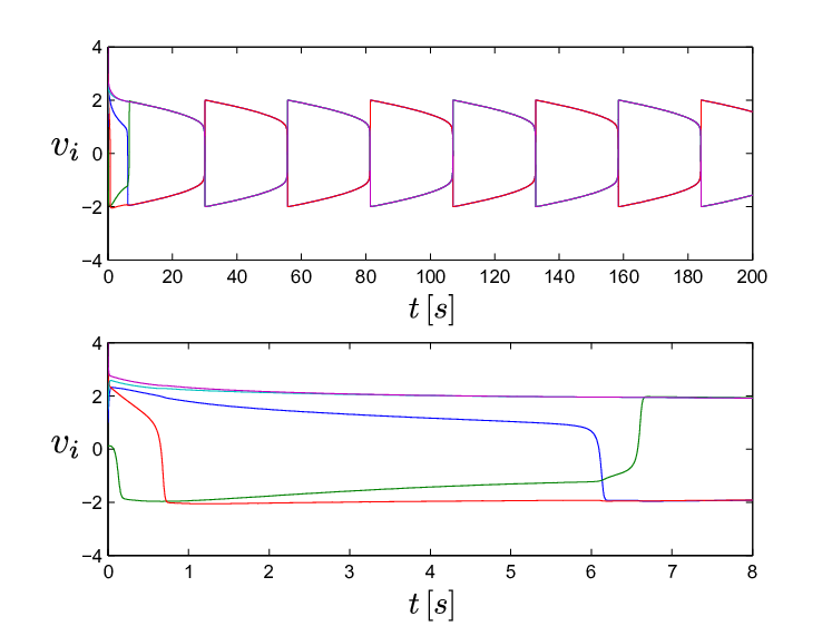
where $v_{i}$ and $w_{i}$ are the membrane potential and the recovery variable for the $i$-th FN oscillator ($i=1,\ldots,N$). In terms of the formalism introduced in Definition 4, anti-synchronization will correspond to the case where $s(t)=-s^{\ast}(t)$ so that $\gamma=-I_{2}$. Now, let $x=[v,w]^{T}$. Then, $f(t,x)=\left[c\left(v+w-\frac{1}{3}v^{3}\right),-\frac{1}{c}(v+bw)\right]^{T}$ fulfills hypothesis H1 of Theorem 2. Consider now the network structure shown in Figure 1 (left panel) and its partition (right panel), obtained by dividing nodes into the two clusters $\mathcal{G}=\{1,3\}$ and $\mathcal{G}^{\ast}=\{2,4,5\}$. The nodes’ dynamics can then be written according to (1) as

It is well know from the literature that the auxiliary network (2) associated to the above dynamics synchronizes if $k$ is sufficiently large [28]. Therefore, by choosing the coupling gain $k$ sufficiently high, hypothesis H3 of Theorem 2 will also be fulfilled. Finally, H2 of Theorem 2 is fulfilled by choosing the coupling functions $g_{ij}$ as: (i) $g_{ij}\left(x_{j}\right)=x_{j}$, if $i,j\in\mathcal{G}$, or if $i,j\in\mathcal{G^{\ast}}$; (ii) $g_{ij}\left(x_{j}\right)=-x_{j}$, if $i\in\mathcal{G}$ and $j\in\mathcal{G}^{\ast}$ or if $i\in\mathcal{G}^{\ast}$ and $j\in\mathcal{G}$. With this choice of the functions $g_{ij}$’s, in accordance to Theorem 2, anti-synchronization is attained with nodes $1$ and $3$ converging onto the same trajectory $s(t)$, while nodes $2$, $4$ and $5$ onto $s^{\ast}=-s(t)$ (see Figure 2).

In order to illustrate the application of Theorem 4, we consider the problem of generating a discrete rotating wave pattern for a network of harmonic oscillators. Specifically, we consider a network of $N=10$ identical harmonic oscillators with topology as in Figure 3 (left panel). The harmonic oscillator dynamics is described by

The symmetries of (15) are those described by rotations by an angle $\phi\in[0,2\pi)$. That is, $\gamma$ belongs to the special orthonormal group $\mathbb{SO}(2)$ or, in matrix form, $\gamma=\begin{bmatrix}\cos\,\phi&-\sin\,\phi\\ \sin\,\phi&\cos\,\phi\end{bmatrix}.$ It is important to note that a set of weakly coupled nonlinear oscillators can be transformed via the so-called phase reduction [29] into a new set of ODEs that is equivariant with respect to the circle group $\mathbb{S}^{1}$, which is isomorphic to $\mathbb{SO}(2)$. To satisfy hypothesis H1 of Theorem 4, consider, for example, three symmetries $\gamma_{1}$, $\gamma_{2}$ and $\gamma_{3}$ associated to rotations by $\phi_{1}=0^{\circ}$, $\phi_{2}=120^{\circ}$ and $\phi_{3}=240^{\circ}$, respectively, and consider the network nodes partitioned into $\mathcal{G}_{1}=\{2,5,7,10\}$, $\mathcal{G}_{2}=\{1,4,6,9\}$ and $\mathcal{G}_{3}=\{3,8\}$ associated to the respective symmetries, as reported in Figure 3 (right panel). Applying the coupling functions in accordance to H2 of Theorem 4, the network dynamics is described by (12) where $F(X)=(I_{N}\otimes A)X$ and the matrix $D$ is the diagonal matrix $D=\mathrm{diag}\,\left\{\gamma_{2},\gamma_{1},\gamma_{3},\gamma_{2},\gamma_{1},\gamma_{2},\gamma_{1},\gamma_{3},\gamma_{2},\gamma_{1}\right\}$. Furthermore, following Theorem $5.1$ in [30], it can be shown that the auxiliary network (13) synchronizes for any $k>0$, and therefore all hypotheses of Theorem 4 are verified. As expected (see Figure 4) the nodes belonging to the same cluster synchronize with each others, with a phase delay of $120^{\circ}$ between the clusters.

References

- [1] Y. Y. Liu, A. L. Barabasi, and J.-J. E. Slotine, “Controllability of complex networks,” Nature, vol. 473, pp. 167–173, 2011.
- [2] A. J. Whalen, S. N. Brennan, T. D. Sauer, and S. J. Schiff, “Observability and controllability of nonlinear networks: The role of symmetry,” Physical Review X, vol. 5, no. 1, p. 011005, 2015.
- [3] G. Chen, “Problems and challenges in control theory under complex dynamical network environments,” Acta Automatica Sinica, vol. 39, pp. 321–321, 2013.
- [4] F. Dorfler and F. Bullo, “Synchronization in complex networks of phase oscillators: a survey,” Automatica, vol. 50, pp. 1539–1564, 2014.
- [5] S. Galam, “Fragmentation versus stability in bimodal coalitions,” Physica A, vol. 230, pp. 174–188, 1996.
- [6] Z. Szallasi, J. Stelling, and V. Periwal, System Modeling in Cellular Biology: From Concepts to Nuts and Bolts. The MIT Press, 2006.
- [7] F. Heider, “Attitudes and cognitive organization,” Journal of Physchology, vol. 21, pp. 107–112, 1946.
- [8] Y. Zhang, G. Hu, H. A. Cerdeira, S. Chen, T. Braun, and Y. Yao, “Partial synchronization and spontaneous spatial ordering in coupled chaotic systems,” Physical Review E, vol. 63, no. 2, p. 026211, 2001.
- [9] A. Pogromsky, G. Santoboni, and H. Nijmeijer, “Partial synchronization: from symmetry towards stability,” Physica D: Nonlinear Phenomena, vol. 172, no. 1–4, pp. 65 – 87, 2002.
- [10] G. Russo and J.-J. E. Slotine, “Symmetries, stability and control in nonlinear systems and networks,” Physical Review E, vol. 84, p. 041929, 2011.
- [11] L. M. Pecora, F. Sorrentino, A. M. Hagerstrom, T. E. Murphy, and R. Roy, “Cluster synchronization and isolated desynchronization in complex networks with symmetries,” Nature communications, vol. 5, 2014.
- [12] C. Altafini, “Consensus problems on networks with antagonistic interactions,” IEEE Transactions on Automatic Control, vol. 58, no. 4, pp. 935–946, 2013.
- [13] M.-C. Fan and H.-T. Zhang, “Bipartite flock control of multi-agent systems,” in Chinese Control Conference (CCC), 2013. IEEE, 2013, pp. 6993–6998.
- [14] H. Zhang and J. Chen, “Bipartite consensus of general linear multi-agent systems,” in American Control Conference (ACC), 2014, 2014, pp. 808–812.
- [15] ——, “Bipartite consensus of multi-agent systems over signed graphs: State feedback and output feedback control approaches,” International Journal of Robust and Nonlinear Control, 2016.
- [16] M. E. Valcher and P. Misra, “On the consensus and bipartite consensus in high-order multi-agent dynamical systems with antagonistic interactions,” Systems & Control Letters, vol. 66, pp. 94–103, 2014.
- [17] A. Proskurnikov, A. Matveev, and M. Cao, “Consensus and polarization in Altafini’s model with bidirectional time-varying topoloties,” in IEEE Conference on Decision and Control, 2014, pp. 2112–2117.
- [18] S. Zhai and Q. Li, “Pinning bipartite synchronization for coupled nonlinear systems with antagonistic interactions and switching topologies,” Systems & Control Letters, vol. 94, pp. 127–132, 2016.
- [19] M. Golubitsky and I. Stewart, The symmetry perspective: from equilibrium to chaos in phase space and physical space. Birkhäuser Verlag, 2002, vol. 200.
- [20] B. Dionne, M. Golubitsky, and I. Stewart, “Coupled cells with internal symmetry: I. Wreath products,” Nonlinearity, vol. 9, no. 2, pp. 559–574, 1996.
- [21] M. Golubitsky and I. Stewart, “Recent advances in symmetric and network dynamics,” Chaos: An Interdisciplinary Journal of Nonlinear Science, vol. 25, no. 9, p. 097612, 2015.
- [22] E. D. Sontag, “Dynamic compensation, parameter identifiability, and equivariances,” PLOS Computational Biology, vol. 13, no. 4, pp. 1–17, 04 2017.
- [23] K. Josić and A. Török, “Network architecture and spatio-temporally symmetric dynamics,” Physica D: Nonlinear Phenomena, vol. 224, no. 1, pp. 52–68, 2006.
- [24] G. Russo and M. di Bernardo, “How to synchronize biological clocks,” Journal of Computationa Biology, vol. 16, pp. 379–393, 2009.
- [25] P. de Lellis, M. di Bernardo, and G. Russo, “On QUAD, Lipschitz and contracting vector fields for consensus and synchronization of networks,” IEEE Transactions on Circuits and Systems I, vol. 58, pp. 576–583, 2011.
- [26] L. M. Pecora and T. L. Carroll, “Master Stability Function for synchronize coupled systems,” Physical Review E, vol. 80, pp. 2019–2112, 1998.
- [27] R. Fitzhugh, “Mathematical models of threshold phenomena in the nerve membrane,” Bulletin of Mathematical Biophysics, 1955.
- [28] S. H. Strogatz, “Exploring complex networks,” Nature, vol. 410, pp. 268–276, 2001.
- [29] Y. Kuramoto, Chemical oscillations, waves, and turbulence. Springer, 1984.
- [30] M. di Bernardo, D. Liuzza, and G. Russo, “Contraction analysis for a class of non differentiable systems with applications to stability and network synchronization,” SIAM Journal on Control and Optimization, vol. 52, pp. 3203–3227, 2014.