Measurement of two-photon exchange effect by comparing elastic cross sections
Abstract
- Background
-
The electromagnetic form factors of the proton measured by unpolarized and polarized electron scattering experiments show a significant disagreement that grows with the squared four momentum transfer (). Calculations have shown that the two measurements can be largely reconciled by accounting for the contributions of two-photon exchange (TPE). TPE effects are not typically included in the standard set of radiative corrections since theoretical calculations of the TPE effects are highly model dependent, and, until recently, no direct evidence of significant TPE effects has been observed.
- Purpose
-
We measured the ratio of positron-proton to electron-proton elastic-scattering cross sections in order to determine the TPE contribution to elastic electron-proton scattering and thereby resolve the proton electric form factor discrepancy.
- Methods
-
We produced a mixed simultaneous electron-positron beam in Jefferson Lab’s Hall B by passing the 5.6 GeV primary electron beam through a radiator to produce a bremsstrahlung photon beam and then passing the photon beam through a convertor to produce electron/positron pairs. The mixed electron-positron (lepton) beam with useful energies from approximately 0.85 to 3.5 GeV then struck a 30-cm long liquid hydrogen (LH2) target located within the CEBAF Large Acceptance Spectrometer (CLAS). By detecting both the scattered leptons and the recoiling protons we identified and reconstructed elastic scattering events and determined the incident lepton energy. A detailed description of the experiment is presented.
- Results
-
We present previously unpublished results for the quantity , the TPE correction to the elastic-scattering cross section, at and 1.45 GeV2 over a large range of virtual photon polarization .
- Conclusions
-
Our results, along with recently published results from VEPP-3, demonstrate a non-zero contribution from TPE effects and are in excellent agreement with the calculations that include TPE effects and largely reconcile the form-factor discrepancy up to GeV2. These data are consistent with an increase in with decreasing at and 1.45 GeV2. There are indications of a slight increase in with .
pacs
14.20.Dh,13.40.Gp,13.60.FzI Introduction
The electromagnetic form factors are the fundamental observables that contain information about the spatial distribution of the charge and magnetization inside the proton. The electric () and magnetic () form factors have been extracted by analyzing data from both unpolarized and polarized electron scattering experiments assuming an exchange of a virtual photon between the electron and the proton while accounting for soft radiative effects and external hard photons.
The unpolarized electron scattering experiments use the Rosenbluth separation method [1, 2, 3, 4, 5, 6], where the elastic cross section is measured at fixed four-momentum transfer, (, where is the incident electron beam energy, is the scattered electron energy, and is the angle of the scattered electron), while varying the electron scattering angle and the incident energy of the electron. The form factors are then extracted from the reduced cross section, given by
| (1) |
where is the cross section for elastic scattering from a point-like proton, is the virtual photon polarization, , and is the proton mass. is then proportional to the -dependence of and is proportional to the cross section extrapolated to .
Recoil polarization experiments [7, 8, 9, 10, 11] measure the polarization of the recoiling proton after scattering a polarized electron off an unpolarized proton target. The ratio of the electric and magnetic form factors is proportional to the ratio of the transverse and longitudinal polarization of the recoil proton. The form-factor ratio can also be extracted from spin-dependent elastic scattering of polarized electrons from polarized protons [12]. The ratio of the electric to magnetic form factors, , where is the proton magnetic moment, extracted from polarized and unpolarized electron scattering shows a significant discrepancy that grows with , as seen in Fig. 1.
A popular explanation is that the observed discrepancy results from neglecting hard two-photon exchange (TPE) corrections [14, 15, 16, 17], a higher-order contribution to the radiative corrections [18, 19, 20]. In TPE, the first exchanged virtual photon can excite the proton to a higher state and the second virtual photon de-excites the proton back to its ground state. TPE will affect the cross section through its interference with the single photon exchange (First Born Approximation) amplitude. This should be smaller than the Born cross section by a factor of . However, the size of the TPE contribution to the cross section is expected to have a significant dependence [21, 22] that grows with , while the -dependent part of the unpolarized cross section in the Born Approximation becomes very small at large .
Calculations of the box and crossed TPE diagrams (Figs. 2(f) and 2(e)) in elastic scattering are complicated since such calculations require complete knowledge of intermediate hadronic states [21, 23, 24, 25, 26, 27, 28, 29, 30, 31]. As a result, these calculations have significant model dependence.
A model-independent way of measuring the size of the TPE effect is by comparing and elastic scattering cross sections [32, 33]. The interference between one- and two-photon exchange diagrams has the opposite sign for electrons and positrons while most of the other radiative corrections are identical for electrons and positrons and cancel to first order in the ratio. Apart from TPE, the only other charge-dependent contribution comes from the interference between the lepton and proton bremsstrahlung radiation terms, which is of comparable size to the TPE effect. Note that the TPE contributions are typically neglected in the correction of electron scattering data except for the infrared-divergent contribution, which is needed to cancel the IR-divergent terms associated with low-energy bremsstrahlung. There are different conventions for how to include the IR-divergent TPE contributions [34, 35], and these yield slight differences in the meaning of the remaining finite TPE contributions [20], referred to here as . In this work, we apply radiative corrections from Ref. [36], which follows the Mo and Tsai convention [34], as do most published extractions of the elastic cross section (with the notable exception of Ref. [37]).
The ratio of the elastic scattering cross sections can be written as
| (2) | |||
| (3) |
where is the total charge-even radiative correction factor and and are the TPE and lepton–proton bremsstrahlung interference contributions. See Ref. [38] for more details. The signs of and are chosen by convention such that they appear as additive corrections for electron scattering. Typically, the experimental ratio is corrected for the calculated and to isolate the TPE contribution:
| (4) |
The measured TPE correction () can be directly used to correct the measured reduced unpolarized elastic scattering cross section, (Eq. 1), as
| (5) |
and then used to extract the TPE-corrected and .
An analysis of Rosenbluth separation data [39] found no non-linear effects in the relationship between and in elastic [6], inelastic, or deep inelastic scattering. Assuming a TPE contribution linearly dependent on , the polarization-Rosenbluth discrepancy can be used to estimate the size of the TPE contributions needed to reconcile them. For above 3-4 GeV2, an -dependent correction of approximately 5% could explain the observed discrepancy [14, 13, 17, 40]. At GeV2 the discrepancy is smaller and provides a less sensitive constraint on TPE contributions [41], though it is consistent with a few % correction.
In the 1960s and 1970s there were several attempts to determine the TPE corrections to electron-proton elastic scattering. Early measurements comparing electron and positron elastic-scattering cross sections [42, 43, 44, 45, 46, 47, 48, 49, 50] were largely limited to low and/or high , where calculations [51, 52, 53] suggest that TPE contributions are small. Given the limited experimental sensitivity of these early measurements, none of the experiments observed a significant deviation from . A global analysis [32] of these measurements showed only limited evidence for non-zero TPE contributions. Improved measurements of these contributions, in particular for large and small values, are required to reconcile the form factor discrepancy.
There have been several recent attempts to make improved TPE measurements by comparing scattering. The VEPP-3 [54, 55] and OLYMPUS [56, 57] experiments used alternating electron and positron beams in storage rings incident on internal gas targets. In these experiments, data for scattering are taken at a fixed beam energy leading to known event kinematics. These experiments measure as a function of lepton scattering angle, which varies both and simultaneously, and do not measure the dependence at fixed . Because the target thickness [58] and hence the luminosity was not well known, both experiments planned to normalize their data to at low and high . The VEPP-3 experiment utilizes a non-magnetic spectrometer while the OLYMPUS experiment utilizes the upgraded BLAST detector that was previously located at MIT-BATES.
The MUSE Collaboration [59] will compare and scattering at very low . This is motivated by the “proton radius puzzle”, the difference between proton radius extractions involving muonic hydrogen [60, 61] and those involving electron-proton interactions [62, 37, 10]. The MUSE experiment will compare electron and muon scattering to look for indications of lepton non-universality, but will also examine TPE corrections, which are important in the radius extraction from electron scattering data [63, 21, 64, 65, 66, 67, 68, 69].
We applied a very different approach to compare and scattering. Rather than alternating between mono-energetic and beams, we generated a mixed beam of positrons and electrons covering a wide range of energies and used the large-acceptance CLAS spectrometer in experimental Hall B at Jefferson Lab to detect both the scattered lepton and the struck proton. The over-constrained elastic-scattering kinematics allowed us to reject inelastic events and to determine the energy of the incident lepton in each event. This allows a simultaneous measurement of electron and positron scattering, while also covering a wide range in and . This paper is a follow up to our previously published results [70] and includes corrections for along with previously unpublished results.
II Experimental Details
This experiment was conducted at the Thomas Jefferson National Accelerator Facility (Jefferson Lab). A simultaneous mixed beam of electrons and positrons was produced using the 5.6 GeV primary electron beam from the accelerator (see Fig. 3). Bremsstrahlung photons were produced by bombarding a radiation length (RL) gold radiator with a 110-140-nA electron beam. The resulting photon beam traversed a 12.7-mm inner-diameter nickel collimator, while the electrons were diverted into the tagger beam dump by the Hall B tagger magnet [71]. The photon beam then struck a 0.09 RL gold converter to produce electron-positron pairs. The mixed lepton-photon beam then passed through a three-dipole magnet chicane. The chicane bent electrons and positrons in the opposite directions, spatially separating them in the horizontal plane (shown as a vertical separation in Fig. 3). The photon beam was stopped by a 4-cm-wide and 35-cm-long tungsten block placed at the upstream face of the second dipole. The electron and positron beams were then recombined into a single beam by the third dipole. The mixed lepton beam then passed through a pair of collimators en route to a 6 cm-diameter, 30-cm long liquid hydrogen (LH2) target. The scattered leptons and the protons were detected in the CEBAF Large Acceptance Spectrometer (CLAS) [72].
The first and third dipoles of the TPE chicane were operated with a magnetic field of T and were about 0.5 m long. They were powered in series by a single power supply. The second dipole had a field of T and was about 1 m long. The momentum acceptance of the chicane is fixed by the width of the photon blocker and the apertures of the second dipole. The width of the photon blocker ( cm) fixed the maximum lepton momentum and the aperture of approximately cm fixed the minimum lepton momentum. In the ideal case the three dipoles are left-right symmetric and the two lepton beams should be identical. The final useful lepton beam energy ranged from approximately 0.5 to 3.5 GeV.
This experiment ran with a much higher primary electron beam current and much thicker radiator than is normally used in CLAS photoproduction experiments and the process of producing a tertiary mixed beam produced a large rate of background radiation in the hall. To protect CLAS from this radiation a number of shielding structures (not shown in Fig. 3) were installed in the hall. Two large shielding structures were constructed between the first and second dipoles of the chicane and between the second and third dipoles of the chicane. A 1-m by 1-m by 0.1-m thick lead wall was placed immediately downstream of the chicane. The lepton beams passed through a 1.75-cm diameter tungsten collimator in this wall. Further downstream just before CLAS was a 4-m by 4-m by 2.5-cm thick steel wall. A second lepton beam clean-up collimator made of lead with a 4-cm diameter aperture was located at the entrance to CLAS. The shielding around the CLAS tagger beam dump was increased during a 2004 test run [38] and remained in place for this experiment. This shielding was designed to remove backgrounds from the beamline and beam dump that would otherwise overwhelm the CLAS detector systems.
| Primary Beam | nA |
|---|---|
| GeV | |
| Radiator (gold) | RL |
| Dist. from target | 21.76 m |
| Photon Collimator | 12.7 mm ID |
| Dist. from target | 15.88 m |
| Converter (gold) | RL |
| Dist. from target | 15.51 m |
| 1st and 3rd Dipoles | T |
| m | |
| 2nd Dipole | T |
| m | |
| Lepton Collimator 1 (tungsten) | 1.75 cm ID |
| Dist. from target | 9.64 m |
| Beam Monitor | 3.12 m |
| Dist. from target | |
| Lepton Collimator 2 (lead) | 4 cm ID |
| Dist. from target | 3.02 m |
| LH2 target | diameter=6 cm |
| length=30 cm | |
| CLAS Torus Current | A |
| Mini-Torus Current | 4000 A |
CLAS (see Fig. 4) is a nearly acceptance detector divided into six segments known as sectors. Six superconducting coils produce a toroidal magnetic field in the azimuthal direction. The magnetic field bends the charged particles towards (in-benders) or away (out-benders) from the beamline. Each CLAS sector contains three regions (R1, R2, and R3) of drift chambers to determine charged particle trajectories [73], a Cherenkov counter (CC) for electron identification [74], time-of-flight (TOF) scintillator counters for timing measurements [75], and an electromagnetic calorimeter (EC) for energy measurements of charged and neutral particles [76]. The CC and EC cover only the forward region of CLAS (). The CLAS event trigger required at least some minimum ionizing energy deposited in the EC in any sector and a hit in the opposite sector TOF. The CC was not used because it is optimized for in-bending particles only and would therefore create a systematic charge bias in lepton detection. Data from the EC was not necessary for particle identification and due to limited angular coverage and the possibility that it would bias the electron-positron comparison, the EC was not used in the analysis. A compact mini-torus magnet (not shown) was placed close to the target to shield the drift chambers from Møller electrons.

A sparse fiber beam monitor (labeled as Beam Monitor in Fig. 3) was installed just upstream of CLAS to measure the position and spatial distribution of the two lepton beams and to monitor their stability during the experiment. The sparse fiber beam monitor contains two sets of 16, mm2 scintillating fibers forming vertical and horizontal grids with a fiber spacing of 5 mm. During commissioning and following each chicane magnetic field reversal, we blocked one of the lepton beams by inserting a remotely-controlled lead block at the entrance of the second chicane dipole. By alternately blocking each one of the two lepton beams, we measured the centroid and shape of the other beam in two dimensions. In order to center both lepton beams at the same position, we determined the position of each individual beam as a function of the current in the first and third chicane dipoles. Figure 5 shows the location of the positron and electron beams as a function of the dipole current. We set the final current at the crossing of the fits to the individual beam positions for both chicane polarities.
We periodically reversed the polarity of the CLAS torus magnets and the beamline chicane magnets to control systematic uncertainties. Periodic torus field reversal provides control on the systematics due to potential detector acceptance related bias for the oppositely charged leptons. Similarly, reversing the chicane current swaps spatial positions of the oppositely charged lepton beams. Data from three such complete polarity cycles and one partial cycle were used in the final analysis. This is discussed in more detail in Sec. III.4.
We determined the energy-dependent lepton fluxes by measuring the energy distributions of the electron and positron beams with the “TPE calorimeter” installed downstream of CLAS. To measure the energy distribution of one lepton beam, we inserted the calorimeter into the beamline, emptied the target, blocked the other beam and reduced the beam intensity by a factor of about by reducing the primary beam current to 1 nA and reducing the radiator thickness to RL.

The TPE Calorimeter consisted of 30 shashlik modules [77] arranged in five rows of six modules each. The individual shashlik modules (Fig. 6) are cm3 and consist of alternating cm2 layers of 1-mm thick lead and 2-mm thick plastic scintillator. Each module has 16 wavelength shifting light-guide fibers, each 1.5 mm in diameter and spaced 7.7 mm apart. The wavelength shifting fibers transmit the light from the individual scintillator layers to photomultiplier tubes. In front of the shashlik modules was a dense fiber monitor (DFM) consisting of a closely-packed array of cm2 scintillating fibers arranged both horizontally and vertically, with an area that covered the face of the calorimeter. We used the DFM to make sure that both lepton beams had the same centroid at the upstream Beam Monitor and at the DFM and were therefore parallel.
We measured the beam-energy distribution for each lepton beam before and after each chicane magnet polarity reversal (see Fig. 7). The energy distributions for electrons and positrons passing through the left side of the chicane are very similar to each other as are the distributions for when the electrons and positrons pass through the right side of the chicane. However, the distributions for leptons passing through the left side of the chicane differ from the distributions of leptons passing through the right side of the chicane, indicating that the chicane was not perfectly left/right symmetric.


In order to know our relative electron and positron luminosities, we rely on several pieces of information:
- •
At GeV energies, electron-positron pair production on the nucleus is the dominant cross section by a factor of [78] and is charge-symmetric.
- •
At energies over 500 MeV, electron and positron interactions with matter are identical (i.e., the annihilation cross section is negligible and the difference between Møller and Bhabha cross sections is negligible) [79].
- •
The magnet current of the beamline chicane where the two lepton beams had the same average location was reproducible to 0.1 A for each magnet cycle.
- •
The ratios of the positron to electron energy distributions for particles passing on one side of the chicane (either left or right) as measured by the TPE Calorimeter are energy independent. This is shown in Fig. 8 where we have plotted the ratio of the incident positron energy distribution to that of the incident electron versus energy for beams through the left (top) and right (middle) sides of the chicane. Monte Carlo simulations of the beamline reproduce this behavior.
- •
The product of the ratios of the positron to electron energy distributions for positive and negative chicane settings as measured by the TPE Calorimeter is also energy independent as seen in the bottom panel of Fig. 8. These electron-positron energy ratios were measured for each chicane flip and were all consistent. Note that the distributions in Fig. 8 are normalized to unity because the separate measurements of and distributions making up the ratios could not be absolutely normalized since we did not have a measurement of the incident primary electron beam charge precise to 1% at the low primary beam currents used to measure the energy distributions.
Detailed GEANT Monte Carlo simulations of the lepton beam transport that included all of the beamline components and materials were conducted prior to the experiment to determine the optimal beamline configuration and to ensure symmetry of the flux and energy of positrons and electrons. The simulations included all electron and positron interactions with matter, including the aforementioned Møller and Bhabha scattering. Various combinations of radiator, converter, and collimation were tested in the simulation to achieve the highest possible lepton flux while also minimizing background. Fig. 9 shows the horizontal () spatial distributions for electrons and positrons at the upstream sparse-fiber beam monitor (BM) and at the target for a single chicane polarity. The RMS of the simulated distributions for both leptons at the beam monitor is 0.96 cm and agreed with online measurements using the beam monitor. An example of a BM measurement for a combined positron/electron beam has been overlaid on the simulated positron histogram (upper left panel). The spike in the histogram to the right of the peak is due to an improperly gain matched fiber. The -distribution RMS increases to 1.1 cm at the upstream face of the target. Fig. 9 also shows that the energy versus distributions are very similar up to about 4.0 GeV but show an asymmetric tilt above 4.0 GeV. However, as stated above, the useful energy range of the lepton beam was limited to about 3.5 GeV. Furthermore, since we measured the electron-proton and positron-proton yields for both positive chicane and negative chicane, any asymmetries in the chicane cancel (see Eq. 15 in Sect. III.4) and the resulting lepton luminosities are equal.

Figure 10 shows the simulated horizontal angular dispersion of the beam at the upstream face of the target as a function of beam energy for a single chicane setting. The mean angle is less than 1rad while the width of the distributions varied from mrad at GeV down to mrad for GeV.

III Data Analysis
The identification of elastic events with no charge bias required us to make a series of cuts and corrections and to test the charge independence of our analysis procedures. This section will discuss the steps taken in the analysis process. These include applying momentum and energy loss corrections, applying data selection cuts, determining dead detector corrections, subtracting backgrounds, and applying radiative corrections.
III.1 Energy loss and momentum corrections
As a charged particle traverses CLAS, it loses energy through interactions with the target and detector materials. The CLAS reconstruction software returns an effective momentum without accounting for this energy loss. For the low momentum protons, this loss could have a significant impact on event reconstruction kinematics. The standard CLAS ELOSS package [80] corrects for this lost energy using the Bethe-Bloch equation to relate the material characteristics and path length to the energy loss. Energy-loss corrections ranged from MeV for protons with momenta above 0.5 GeV up to MeV for momenta down to 0.2 GeV. No energy loss corrections were done for leptons.
Because of incomplete knowledge of the magnetic field and drift chamber positions in CLAS, the reconstructed momenta show some systematic deviations. To determine the momentum corrections, a set of runs was taken with a 2.258-GeV primary electron beam incident directly on the CLAS target. Data were taken with both torus polarities. We then used exclusive events where all the final-state particles were detected and employed four-momentum conservation to determine the correct scattering angles and magnitudes of the momenta. The events used were and events. This combination of particles provided the same scattering-angle and momenta ranges as seen in the final data as well as providing events with both positive and negative charge. The momentum corrections were less than 1% of the momentum and ultimately lead to an invariant mass distribution for electron-proton elastic scattering that is consistent with the proton mass to within less than 1 MeV. Imprecision in the momentum corrections was unimportant because we used the measured lepton and proton momenta to select elastic scattering events (see below) but not to calculate any of the kinematic quantities of the elastic events.
III.2 Data selection cuts
We applied a series of cuts to the data to select elastic events. In addition to the kinematic cuts described below, a 28-cm target vertex cut was applied to both lepton and proton candidates to remove events from the target walls. We explored using cuts on the transverse target vertex and the distance of closest approach between the lepton and proton but saw no effect on the final data set. A set of momentum-dependent fiducial cuts on the angles (both and ) were applied to select the region of CLAS with uniform acceptance. The cuts remove the sector edges were the detection efficiency varies rapidly. The cuts are necessary because the acceptance of CLAS is different for the two lepton charges and were selected such that the angular acceptance of both positrons and electrons were identical for both torus polarities. The cut was chosen to be the minimum angle for the out-bending particle and varied from about 15∘ for leptons of 1.5 GeV to about 20∘ for leptons of 0.8 GeV (the minimum energy used in this analysis).
This analysis did not use the usual EC- and CC-based CLAS lepton identification scheme. These detector components cover only a limited range of scattering angles. We instead employed elastic scattering kinematics, which are over-constrained by the simultaneous detection of both the lepton and the proton.
The elastic event identification algorithm is shown in Fig. 11 and started with the selection of the events with at least two good tracks in opposite sectors of CLAS. Ideally, events with only two tracks would be selected. However, events triggered by accidental hits in conjunction with a valid elastic event could have more than two tracks. In that case, pairs of viable tracks were formed by looping over all possible good track pairs in the event that had either a negative/positive or positive/positive charge combination. For a pair with a negative/positive charge combination: the negative track was considered as a candidate and the positive track as a candidate. If the pair passed all elastic kinematic cuts discussed in the next section, the pair was identified as the elastic pair. If not, the next track pair of the event was considered. For positive/positive pairs, we first considered one of the tracks to be the candidate and the other to be candidate. We then checked to see whether the pair passed elastic kinematic cuts as or as . If the pair passed kinematic cuts both as and as , an additional minimum-timing cross check was done. This cross check used the difference between the TOF of the particle pairs ( proton TOF lepton TOF) and compared it to TOF difference () calculated assuming the pair was (pair 1) or (pair 2). Whichever pair assumption that led to the smallest difference ( or 2) was assigned to the event. Overall, a negligible fraction of events () had more than one pair passing all cuts. We note that no TOF cuts were applied and that all cuts for and events were identical in order to avoid introduction of a charge bias.

III.2.1 Elastic Kinematic Cuts
Because elastic scattering kinematics are overdetermined by measuring momenta and angles for both leptons and protons, we can identify elastic events and determine the incident lepton energy by a series of four kinematic cuts.
- 1.
Co-planarity cut: The elastically scattered lepton and proton are co-planar. As a result, the azimuthal angle difference between the lepton and the proton () was sharply peaked at 180∘ (Fig. 12, upper left).
- 2.
Lepton Energy Cuts: The unknown energy of the incident lepton can be reconstructed using the scattering angles of the lepton () and the proton () as,
(6) The incident lepton energy can also be calculated using the momenta of the lepton () and the proton () and their scattering angles as,
(7) has better precision and accuracy than because the scattering angles are better determined by CLAS than the momentum. Kinematic variables such as and , which require knowledge of the beam and scattered lepton energies were calculated using and . Figure 13 shows the beam energy for and reconstructed using Eq. 6. A beam-energy cut of GeV was applied to avoid the lower energies where the energy distribution is changing rapidly.

Figure 13: (Color online) Reconstructed incident beam energy distributions of all elastic scattering events using scattering angles. The positron (red) and electron (blue) distributions have been scaled by the total number of counts in the distributions and show almost imperceptible differences. This figure differs from Fig. 7 in that it shows the incident energy distribution for elastic scattering events rather than the overall beam energy distribution. For perfect momentum and angle reconstruction, Eqs. 6 and 7 yield the same result,
(8) The energy of the elastically scattered lepton can be calculated using the incident energy and the scattering angle as,
(9) For perfect reconstruction, the difference between the CLAS-measured scattered lepton energy () and the energy calculated by Eq. 9 should be zero:
(10) Fig. 14 shows that and are linearly correlated. Rather than applying cuts to these variables, the optimal, uncorrelated cuts are on their sums () and their differences (). Distributions for and are shown in the bottom panels of Fig. 12.

Figure 14: (Color online) and distributions for candidate events prior to application of kinematic cuts showing the linear correlation between vs. . An identical correlation is seen for events. - 3.
Proton Momentum Difference Cut: The momentum of the recoil proton was calculated using the lepton and proton scattering angles along with the angle-determined recoil lepton energy as
(11) A cut was placed on the difference between the measured and calculated proton momenta (). The difference is shown in the upper right panel of Fig. 12.
In each case, the widths of the distributions vary with and . Based on the means and widths of Gaussian fits to the peaks of the distributions, - and -dependent, parameterized cuts were set to . Fig. 12 shows distributions of the four cut variables before and after applying cuts on other three variables. The effect of the other three cuts on any one variable leads to distributions that are remarkably free of background for all but kinematic regions corresponding to large electron angles (see Sec. III.5). The non-Gaussian shape of the distribution in Fig 11 is due to summing over the entire kinematic range, where the width and background distributions are changing. The positive offset in is due to the fact that (Eq. 9) is offset in the negative direction because of imperfections in the momentum corrections leading to being less than . For each kinematic bin (see, e.g., Fig. 18) the signal peak is Gaussian, but the background is not.
III.3 Kinematic coverage and binning
Figure 15 shows the and distribution of elastic scattering events for positive torus polarity. The wide coverage of and is apparent. There is a hole in the distribution at and lower values of . This hole is due to the trigger used in the experiment, which required one particle track hitting the forward TOF and the EC. Events where neither particle had a lab-frame scattering angle of less than about 45∘ did not trigger the CLAS readout. The trigger hole is largest for , positive torus events, which ultimately limits our kinematic coverage.
The data bins (Fig. 15) were selected to measure the dependence of at two values of and the dependence of at two values of with roughly equal statistical uncertainties in each range. We avoided the edges of the distributions, where the acceptance for in-bending and out-bending particles vary rapidly. The binning choice leads to some overlap in the data bins. The average values, and , are given in Tables 2 and 3.

III.4 Dead detector removal and acceptance matching
In addition to the fiducial cuts mentioned above, we also removed dead, broken, and/or inefficient detector elements of CLAS as these components could lead to charge-dependent biases in the lepton detection efficiency. Events that hit inefficient TOF paddles were removed. The forward region of one of the six sectors of CLAS (sector 3) had a large number of holes due to dead drift chamber and EC channels. All data with either particle entering this region of sector 3 were removed from the analysis as such events would have insufficient information for event reconstruction.
As mentioned above, the polarities of the CLAS torus magnets and the beamline chicane magnets were periodically reversed during the course of the experiment. For a given torus polarity, , and chicane polarity, , we measured the ratio of detected elastically-scattered positrons, , and electrons, :
| (12) |
Any proton acceptance and detector efficiency factors were the same for both lepton charges and cancel in this ratio. The yield is proportional to the elastic-scattering cross section, (here refers to the lepton charge), the lepton-charge-related detector efficiency and acceptance function, , as well as chicane-related luminosity factors, , so that
| (13) |
Taking the square root of the product of measurements done with both torus polarities but a fixed chicane polarity gives
| (14) | |||||
where we assume that and . That is, the unknown detector efficiency and acceptance functions for positrons cancel those for electrons when the torus polarity is switched and are expected to cancel out in this double ratio. The validity of this cancellation is discussed in more detail below.
Reversing the chicane current swaps the spatial positions of the oppositely charged lepton beams so that and . Then taking the square root of the product of the double ratios defined in Eq. 14 leads to
| (15) | |||||
By taking data with both chicane polarities, any flux-dependent differences between the two lepton beams is eliminated within the uncertainty. Each complete cycle of chicane and torus polarity reversal contained all four configurations (, , , ).
This experiment relies on the fact that the electron and positron acceptance factors () cancel out in Eq. 14. However, inefficient detectors can bias the lepton detection efficiencies. This effect was taken into account by implementing a “swimming” algorithm to ensure the same detection efficiencies in each TOF paddle. For each event, this algorithm traced the particle trajectories through the CLAS geometry and the magnetic field (including the mini-torus field) and predicted the hit positions on the detectors. The algorithm was then rerun with the conjugate lepton charge, keeping the momentum and scattering angle unchanged. The event was accepted only if both the actual lepton and its conjugate are within the fiducial acceptance region and hit a good TOF paddle. Otherwise, the event was rejected. The typical change to the final results from applying the swimming algorithm was about %.
The angles and the momenta of the lepton and proton in each event are not independent of each other. These correlations can potentially interfere with the acceptance canceling as described in Eqs. 13 and 14. In addition, the minitorus magnetic field, used to deflect Moller electrons, was never reversed. We simulated events using a Monte Carlo program in order to determine the magnitude of these effects on our quadruple ratios.
The energy distributions of the incident lepton beams were taken from a detailed GEANT-4 simulation of the beamline, including the radiator, convertor, tagger and chicane magnets, collimators, and shielding. Lepton-proton elastic scattering events were thrown uniformly in phase space and then weighted by the cross section. This allowed us to get a realistic distribution of events with high statistics for all bins in a reasonable time period. Once generated, the Monte Carlo data were analyzed with the same analysis routine as the experimental data.
For each bin, we calculated the acceptances for positive and negative torus fields and for electron-proton and positron-proton events separately as the ratio of weighted reconstructed events (selected with the same analysis procedure as the data) to weighted generated events:
| (16) |
where the subscript on refers to the torus polarity and the superscript refers to the lepton charge. We calculated the uncertainty for each acceptance using weighted binomial uncertainties and then combined the acceptances to get the acceptance correction factor as
| (17) |
We then divided the quadruple ratios (Eq. 15) with this acceptance correction factor.
The acceptance correction factors for the final kinematic points are shown in Fig. 16. The acceptance correction factors are all within 0.5% of unity and almost all are compatible with unity. The statistical uncertainties are all less than or equal to 0.1%. Therefore, the effects of the minitorus and of lepton-proton kinematic correlations are very small.
III.5 Background Subtraction
After applying all event selection cuts some background remains, particularly at low and high . The background was found to be symmetric about but not symmetric in or . Therefore, we used the distributions to determine the background. distributions were made for each bin and for and events separately. The tails of the distributions (over the regions and ) were fit with a Gaussian. Fig. 17 shows the Gaussian background fit for the bin with the most background.
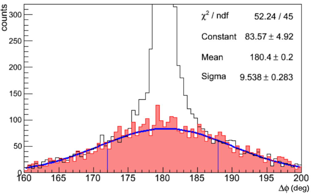
To verify the Gaussian shape of the background, we used a sampling method to determine the shape of the background at low . Figure 18 shows the distribution for . The sample was selected from the right-hand tail of the distribution and scaled to match the tails of the distributions. The sampled background shown by the red histogram in Fig. 17 shows excellent agreement with the tails of the distribution and also with the Gaussian background fit. The distribution for events (not shown) at the same kinematics is similar in shape but with background that is 5-10% smaller than for the events. However, the sampled background for events also matches Gaussian background fit. At higher the peak broadened significantly and the background was much smaller so it was not possible to use the sampling method. In bins where it was possible to use both methods we found that the final result for was the same to within statistical uncertainties, therefore, the Gaussian fit was employed for all bins.

III.6 Radiative Corrections
Higher order QED diagrams beyond the Born approximation have a significant, but generally well-calculable, impact on the elastic charged lepton–proton scattering cross sections. The largest contributions are the charge-even terms, which are the same for electrons and positrons. The charge-odd terms cause the difference between the positron and electron scattering cross sections while the charge even terms dilute this difference.
There are two leading order corrections that are odd in the product of the beam and target charges. The first is the TPE contribution (or more correctly, the interference between one- and two-photon exchange amplitudes), which is highly model-dependent, and which we aim to extract. The second is the interference between real photon emission from the proton and from the incident or scattered electron. The latter is considered a background for this measurement and needs to be computed to isolate the TPE contribution.
The bremsstrahlung interference term is somewhat model dependent, as the proton bremsstrahlung contribution has some sensitivity to the proton internal structure. However, this sensitivity is relatively small and the amplitude for photon emission from the proton is also small at low , where the proton is not highly relativistic.
While the key contribution is the charge-odd bremsstrahlung term, the charge-even terms also need to be applied, as they dilute the charge-odd term as shown in Eq. 2. For both contributions, the bremsstrahlung contributions are typically calculated assuming a fixed energy loss or cut used to determine which events are included as elastic and which are in the excluded radiative tail. In our case, we apply our elastic event identification kinematic cuts, rather than a cut. The primary difference between the two approaches is that our cuts do not remove events where the incoming lepton radiates a photon; this radiation just changes the incident lepton energy.
We simulated radiative effects following the prescription of Ref. [36], taking the “extended peaking approximation” approach. In this approach, radiated photons are generated only in the directions of the charged particles, but both the incoming and outgoing leptons and the struck proton are all allowed to radiate. The sum of the radiated photon energy thus has a fairly realistic angular distribution, as shown in Ref. [36, 81].
The Monte Carlo simulation was run twice for electrons with the radiative effects turned on and off, then twice more for positrons with the radiative effects turned off and on, resulting in ratios of yields given by
| (18) |
In each of the simulations we assumed no TPE effects. We then define a charge-odd correction factor
| (19) | |||||
| (20) |
To within any detector acceptance effects, the terms of cancel in this ratio. One sees that still has a contribution from .
We obtained the charge-even radiative correction by averaging the results of the simulation leading to
| (21) | |||||
This can be used to extract the charge-odd term, , from Eq. 20. Figure 19 shows the charge-odd (top panels) and charge-even (bottom panels) bin-averaged radiative corrections. We can then extract from the measured to cross section ratio of Eq. 2 using and and use that to determine as defined in Eq. 4.
Any error due to the radiative corrections prescription is likely to have a correlated effect between different kinematics. Because the correlation is unknown, we approximate this by applying an overall scale uncertainty of 0.3% (roughly 15% of the correction at the high kinematics), with an additional point-to-point uncertainty at each setting equal to 15% of the correction for that point.
| Bin No. | |||||||||||
|---|---|---|---|---|---|---|---|---|---|---|---|
| 1 | 0.84 | 0.39 | 0.0100 | 0.0030 | 0.0013 | 0.0159 | 0.0054 | 0.0075 | 0.0001 | 0.001 | 0.0212 |
| 2 | 0.86 | 0.51 | 0.0034 | 0.0030 | 0.0013 | 0.0074 | 0.0010 | 0.0112 | 0.0001 | 0.001 | 0.0143 |
| 3 | 0.85 | 0.83 | 0.0034 | 0.0030 | 0.0013 | 0.0021 | 0.0030 | 0.0027 | 0.0014 | 0.001 | 0.0068 |
| 4 | 0.85 | 0.91 | 0.0034 | 0.0030 | 0.0013 | 0.0015 | 0.0024 | 0.0005 | 0.0014 | 0.001 | 0.0058 |
| 5 | 1.44 | 0.40 | 0.0034 | 0.0030 | 0.0013 | 0.0070 | 0.0023 | 0.0031 | 0.0003 | 0.001 | 0.0093 |
| 6 | 1.45 | 0.60 | 0.0034 | 0.0030 | 0.0013 | 0.0069 | 0.0021 | 0.0004 | 0.0005 | 0.001 | 0.0087 |
| 7 | 1.46 | 0.76 | 0.0034 | 0.0030 | 0.0013 | 0.0075 | 0.0024 | 0.0021 | 0.0005 | 0.001 | 0.0095 |
| 8 | 1.47 | 0.83 | 0.0034 | 0.0030 | 0.0013 | 0.0012 | 0.0014 | 0.0015 | 0.0046 | 0.001 | 0.0071 |
| 9 | 1.47 | 0.90 | 0.0034 | 0.0030 | 0.0013 | 0.0043 | 0.0021 | 0.0024 | 0.0057 | 0.001 | 0.0092 |
| 10 | 0.72 | 0.45 | 0.0034 | 0.0030 | 0.0013 | 0.0033 | 0.0033 | 0.0003 | 0.0001 | 0.001 | 0.0067 |
| 11 | 0.89 | 0.45 | 0.0034 | 0.0030 | 0.0013 | 0.0132 | 0.0034 | 0.0057 | 0.0001 | 0.001 | 0.0155 |
| 12 | 1.14 | 0.45 | 0.0034 | 0.0030 | 0.0013 | 0.0037 | 0.0071 | 0.0015 | 0.0004 | 0.001 | 0.0095 |
| 13 | 1.73 | 0.45 | 0.0034 | 0.0030 | 0.0013 | 0.0063 | 0.0115 | 0.0012 | 0.0007 | 0.001 | 0.0140 |
| 14 | 0.23 | 0.92 | 0.0034 | 0.0030 | 0.0013 | 0.0012 | 0.0028 | 0.0003 | 0.0013 | 0.001 | 0.0059 |
| 15 | 0.34 | 0.89 | 0.0034 | 0.0030 | 0.0013 | 0.0005 | 0.0005 | 0.0002 | 0.0006 | 0.001 | 0.0049 |
| 16 | 0.45 | 0.89 | 0.0034 | 0.0030 | 0.0013 | 0.0007 | 0.0010 | 0.0002 | 0.0002 | 0.001 | 0.0050 |
| 17 | 0.63 | 0.88 | 0.0034 | 0.0030 | 0.0013 | 0.0011 | 0.0052 | 0.0006 | 0.0005 | 0.001 | 0.0072 |
| 18 | 0.89 | 0.88 | 0.0034 | 0.0030 | 0.0013 | 0.0017 | 0.0032 | 0.0008 | 0.0011 | 0.001 | 0.0062 |
| 19 | 1.42 | 0.87 | 0.0034 | 0.0030 | 0.0013 | 0.0016 | 0.0022 | 0.0016 | 0.0041 | 0.001 | 0.0071 |
III.7 Systematic Uncertainties
As discussed earlier, our experimental design helped to cancel or minimize most of the systematic uncertainties in the measurement of . Any remnant systematic uncertainties are discussed below. Table 2 lists the various sources of systematic uncertainty on the measured ratio before doing radiative corrections. The effect of these corrections is to reduce the measured ratio by a factor of , so it similarly will reduce the total systematic uncertainty in .
- 1.
CLAS imperfections: We compared our final cross section ratio measured in different sectors of CLAS. The variations in these ratios quantify the systematic effects due to detector imperfections. Since we removed the forward going lepton or proton events from sector 3, we had five independent cross-section ratios for each bin. We calculated the weighted average and the chi-squared based on the scatter of the five independent ratios. We then added the same systematic uncertainty to each of the sector-based quadruple ratios and recalculated the chi-squared and the confidence level. We chose a 0.75% systematic uncertainty for each sector measurement to give an average confidence level of % for all of the bins. This gives a sector-to-sector overall systematic uncertainty of for each bin except bin 1 as it showed a larger sector dependence than the other bins. This uncertainty is listed in Table 2 under .
- 2.
Differences in the and luminosities: With electron-positron pair production being inherently charge symmetric, the and beam fluxes should be identical. In the experiment, the only differences in the two beams could come from differences in beam transport from the converter to the target. The chicane magnet setting was periodically reversed several times during the run period to minimize the differences and we measured the energy distributions of the electron and positrons with TPE Calorimeter after each reversal. Fig. 13 shows that the reconstructed energy distributions of the incident and are identical. Any difference in the incident lepton flux primarily appears as the variation in the cross section ratios for the different chicane cycles. The systematic uncertainty was calculated similarly to that for the CLAS imperfections. For each of the independent chicane cycles we determined the double ratios (Eq. 14). We added the same systematic uncertainty to each double ratio to give an average confidence level of 50% for all bins. The overall systematic uncertainty due to lepton luminosity differences was estimated to be 0.3% for each bin. It is listed in Table 2 under .
- 3.
Charge independence of track reconstruction: A series of special runs were conducted with the CLAS minitorus turned off in order to make sure that our track reconstruction and analysis code was independent of the charge of the particles. We determined the number of elastic events for positive and negative torus settings and a fixed chicane setting. We then replayed the same runs assuming the opposite torus polarity, thus reversing the roles of negatively and positively charged tracks, and determined the number of elastic events where both particles had a “negative” charge. The analysis found equal numbers of events for the two analyses to within 0.13%, which we have assumed as a systematic uncertainty associated with the charge dependence of track reconstruction. It is listed in Table 2 under .
- 4.
Elastic event selection and background subtraction: For each bin, the systematic uncertainty due to elastic event selection cuts was estimated by increasing the width of the kinematic cuts from the nominal cuts to cuts. Relaxing these cuts doubled the background present in the data. Thus the kinematic cut uncertainty includes the background subtraction uncertainty. The deviation of the final ratio with the varied cuts from the ratio with the nominal cuts was assigned as the systematic uncertainty due to our event selection. It is listed in Table 2 under .
- 5.
Background fitting: We determined the systematic uncertainty due to background fitting by varying the fitting regions from the nominal fitting range. For each bin, we varied the fitting range by (160∘ to 170∘ and 190∘ to 200∘) and (160∘ to 174∘ and 186∘ to 200∘) and recalculated the final ratios. The systematic uncertainty due to the background subtraction was estimated to be the average deviation of the varied ratios () from that with the nominal fitting ranges ():
(22) - 6.
Target vertex cut: For each bin, the systematic uncertainty due to the target vertex cut was estimated by varying the width of the nominal vertex cut of cm to cm. The deviation of the final ratio with the varied cuts from the ratio with the nominal cut was assigned as the systematic uncertainty due to the vertex cut. It is listed in Table 2 under .
- 7.
Fiducial cuts: The systematics effect due to the applied fiducial cuts were estimated by increasing the lower limit of the cut by one degree and decreasing the upper limit of cut by one degree thereby reducing the fiducial volume. The deviation of the final ratio with the tightened fiducial volume from that with the nominal fiducial volume was assigned as the systematic uncertainty due to our fiducial cuts. It is listed in Table 2 under .
- 8.
Acceptance correction: As seen above, the acceptance correction factors determined from the Monte Carlo simulation were close to unity with a high level of uniformity. We conservatively estimate an uncertainty of 0.1% for all bins, which is 20% of the largest deviation of the acceptance correction from unity. It is listed in Table 2 under .
For each bin, the contribution from all the sources were added in quadrature to obtain our total systematic uncertainties . The total uncertainties are presented along with the final results in Table 3.
IV RESULTS
The final results are given in Table 3 along with all associated uncertainties, and shown in Figs. 20 and 21. Table 3 includes both , which is the experimentally measured equivalent to of Eq. 2, and which is the radiatively-corrected result as shown in Eq. 4. Estimated systematic uncertainties associated with the and corrections are also given in the table. The numbers in the column labeled “overlap” indicate that a given bin contains part or all of the bins listed in that column of the table. For example, bin 1 has an overlap with part of bin 10, while bin 10 overlaps both bins 1 and 2. The reason for showing data from overlapping kinematic bins is to separately study the and dependencies, though future use of our results in modeling TPE corrections should take into account the fact that we are displaying non-independent results. Quantitative model comparisons will be discussed in Sec. IV.4.
| Bin No. | overlap | |||||||||
| 1 | 0.84 | 0.39 | 1.0268 | 1.0070 | 0.0122 | 0.0043 | 0.0182 | 0.0223 | 0.003 | 10 |
| 2 | 0.86 | 0.52 | 1.0057 | 0.9896 | 0.0109 | 0.0024 | 0.0122 | 0.0166 | 0.003 | 10 |
| 3 | 0.85 | 0.83 | 1.0226 | 1.0074 | 0.0066 | 0.0032 | 0.0055 | 0.0092 | 0.003 | 18 |
| 4 | 0.85 | 0.91 | 1.0074 | 0.9976 | 0.0054 | 0.0015 | 0.0047 | 0.0073 | 0.003 | 18 |
| 5 | 1.44 | 0.40 | 1.0623 | 1.0282 | 0.0102 | 0.0086 | 0.0075 | 0.0153 | 0.003 | 11,12,13 |
| 6 | 1.45 | 0.60 | 1.0299 | 1.0047 | 0.0131 | 0.0047 | 0.0070 | 0.0155 | 0.003 | 11,12,13 |
| 7 | 1.46 | 0.76 | 1.0120 | 0.9943 | 0.0109 | 0.0027 | 0.0075 | 0.0135 | 0.003 | |
| 8 | 1.47 | 0.83 | 1.0134 | 0.9956 | 0.0122 | 0.0028 | 0.0056 | 0.0137 | 0.003 | 19 |
| 9 | 1.47 | 0.90 | 1.0010 | 0.9965 | 0.0111 | 0.0007 | 0.0072 | 0.0132 | 0.003 | 19 |
| 10 | 0.72 | 0.45 | 1.0224 | 1.0052 | 0.0113 | 0.0036 | 0.0058 | 0.0132 | 0.003 | 1,2 |
| 11 | 0.89 | 0.45 | 1.0246 | 1.0009 | 0.0110 | 0.0044 | 0.0132 | 0.0178 | 0.003 | 5,6 |
| 12 | 1.14 | 0.45 | 1.0490 | 1.0239 | 0.0112 | 0.0067 | 0.0078 | 0.0152 | 0.003 | 5,6 |
| 13 | 1.73 | 0.45 | 1.0427 | 1.0176 | 0.0118 | 0.0059 | 0.0113 | 0.0173 | 0.003 | 5,6 |
| 14 | 0.23 | 0.92 | 0.9950 | 0.9920 | 0.0020 | 0.0008 | 0.0052 | 0.0056 | 0.003 | |
| 15 | 0.34 | 0.89 | 0.9940 | 0.9888 | 0.0022 | 0.0012 | 0.0043 | 0.0050 | 0.003 | |
| 16 | 0.45 | 0.89 | 1.0040 | 0.9974 | 0.0022 | 0.0010 | 0.0043 | 0.0049 | 0.003 | |
| 17 | 0.63 | 0.89 | 1.0130 | 1.0025 | 0.0029 | 0.0020 | 0.0059 | 0.0069 | 0.003 | |
| 18 | 0.89 | 0.88 | 1.0240 | 1.0097 | 0.0036 | 0.0032 | 0.0049 | 0.0069 | 0.003 | 3,4 |
| 19 | 1.42 | 0.87 | 1.0150 | 1.0000 | 0.0067 | 0.0026 | 0.0057 | 0.0092 | 0.003 | 8,9 |
IV.1 -dependence
Fig. 20 shows the -dependence of at and 1.45 GeV2, along with previous world data and the calculations of Refs. [21, 31, 20]. Our results at = 0.85 GeV2 are consistent with no epsilon dependence, though inclusion of the VEPP-3 results at and 0.976 GeV2 may suggest a slight increase of with decreasing . Our data at = 1.45 GeV2 when combined with the VEPP-3 = 1.51 GeV2 result show a moderate epsilon dependence. Together with the VEPP-3 data, the results are inconsistent with the no-TPE () limit.
The data are compared to calculations of TPE in a hadronic framework [21, 31], and the analytic results for scattering from a structureless (point-like) proton [20]. The data are significantly higher than the point-proton calculation and show the opposite dependence. The data are consistent with the hadronic calculations which, for the values presented here, are dominated by the elastic intermediate state. The hadronic calculations bring the form factor ratio extracted from Rosenbluth separation measurements into good agreement with the polarization transfer measurements up to GeV2 [20], so the data support the explanation of the discrepancy in terms of TPE contributions. As discussed in Ref. [18], confirmation that TPE contributions explain the discrepancy is sufficient to allow extraction of the form factors without a significant uncertainty associated with the TPE corrections.
IV.2 -dependence
Fig. 21 shows the -dependence of the ratio at and 0.88 along with previous world data and the calculations of Refs. [21, 31, 20]. In both cases our results are consistent with little or no dependence, while the inclusion of the VEPP-3 data at indicates a gradual increase in with . As before, the results are largely consistent with the calculations of Blunden et al. and Zhou and Yang but not that for a point-like proton.
IV.3 TPE Corrected Rosenbluth Extraction at GeV2
From our results of at GeV2 we determined the correction factor . We did a linear fit of all of the data shown in Fig. 20 that was constrained to go to at . We then applied the resulting correction factor (see Eq. 5), including fit uncertainties, to the unpolarized reduced cross section of Andivahis et al. [2] and did a Rosenbluth separation to extract at GeV2. Figure 22 shows the original reduced cross section measurements from Andivahis et al. and the CLAS TPE corrected values as a function of . The TPE corrections change the proton form factor ratio obtained from the unpolarized data from to , bringing it into agreement with the polarization transfer result of at GeV2 by Punjabi et al. [7].
IV.4 Global Analysis
In Ref. [70], we examined the sensitivity of the high- and high- data (without the VEPP-3 points), and found that they favored the hadronic TPE calculations [21, 31] over the no-TPE hypothesis by 2.5. The analysis here includes the full CLAS kinematic coverage, which includes additional data at lower values. These additional data have large uncertainties and are in the kinematic region where the TPE calculations have minimal disagreement, and so have a limited impact in testing different TPE hypotheses. However, combining the VEPP-3 results, along with the full CLAS data set, yields a more significant test of the TPE calculations under the assumption that any missing charge-even corrections to the VEPP-3 results are minimal. Though other calculations of TPE effects are available (e.g. GPD-based calculations of ref. [16]), the hadronic calculations are expected to be more reliable at this low-to-moderate range. To make a more quantitative comparison of the TPE calculations, we perform a global comparison of the data to the hadronic calculations of Refs.[21, 31], the no-TPE assumption, and the calculation based on a structureless proton [20].
Our data points and the VEPP-3 measurements have uncertainties that are at the 0.5-1.8% level. Previous measurements typically have uncertainties greater than 3%, and the measurements with better uncertainties are generally at GeV2 or , where the calculations all suggest minimal TPE contributions. Because of the large experimental uncertainties leading to low sensitivity, as well as incomplete knowledge of how radiative corrections were applied to extract , we do not include these points in our analysis.
| TPE calculation | Conf. Level | |
|---|---|---|
| Blunden () [21] | 1.23 | 23.5% |
| Zhou & Yang () [31] | 1.27 | 20.8% |
| Zhou & Yang () [31] | 1.19 | 27.0% |
| (No TPE) | 2.32 | 0.20% |
| Point-proton calculation | 7.38 | % |
For this analysis, we have to select a subset of our data, to avoid double counting of data included in more than one binning scheme. We take the high- data (bins 5–9) and the high- data (bins 14–18, excluding bin 19 which overlaps bins 8 and 9). We also include the two low-, low- data points (bins 1 and 2), which do not overlap with the bins at high- or high-. This yields a total of 12 data points from our measurement. For the Novosibirsk data, we use the four non-normalization data points, including a 0.3% systematic uncertainty applied to account for the model-dependence of the high- normalization procedure. The comparison of the CLAS plus VEPP-3 data (16 data points total) to the various models is summarized in Table 4. We find that the addition of the CLAS data points that were not presented in our previous publication [70] do not significantly impact the comparison to the models but the addition of the VEPP-3 data yields a significant improvement. The data are in good agreement with the hadronic calculations of Ref. [21, 31] but of insufficient precision to make any definitive distinction between them. However, the data exclude the no-TPE hypothesis at the level, and rule out the point-proton result at the level. The point-proton model is essentially equivalent to the limit, which is insensitive to proton structure, used to approximate TPE corrections at low values [37]. The fit includes a variation of the normalization uncertainty associated with the model dependence of the radiative corrections, which increases all of the CLAS ratios by roughly 0.3% for the fit to the hadronic calculation and decreases it by a similar amount for the point-like comparison.
V Conclusions
Our results, along with recently published results from VEPP-3, rule out the zero TPE effect hypothesis at the 99.8% confidence level and are in excellent agreement ( to 1.27) with the calculations [21, 31] that include TPE effects and largely reconcile the form-factor discrepancy. The combined CLAS and VEPP-3 data are consistent with an increase in with decreasing at and 1.45 GeV2. A slight, non-statistically significant, increase in with is seen. Extracting the -dependent TPE correction factor, , from our results for at GeV2 and applying it to the extraction of at GeV2 from the Ref. [2] reduced cross-section data brings it into good agreement with the polarization transfer measurement at GeV2 by Punjabi et al. [7].
Our data, together with those of VEPP-3, show that TPE effects are present and are large enough to explain the proton electric form factor discrepancy up to GeV2. Since this paper was submitted, the OLYMPUS results have been published [57]. A recent review article [82] in which all three of the modern data sets were included in a global analysis came to a similar conclusion. However, the form factor discrepancy is small at the low momentum transfers of the new data. Though there are currently no experiments planned to extend the measurements to GeV2, where the form-factor discrepancy is the largest, such experiments are needed before one can definitively state that TPE effects are the reason for the discrepancy.
Acknowledgements.
We thank Bernard Mecking, the former Jefferson Lab Hall B leader, for suggesting this innovative experimental technique. We acknowledge the outstanding efforts of the Jefferson Lab staff (especially Dave Kashy and the CLAS technical staff) that made this experiment possible. This work was supported in part by the U.S. Department of Energy and National Science Foundation, the Italian Istituto Nazionale di Fisica Nucleare, the Chilean Comisión Nacional de Investigación Científica y Tecnológica (CONICYT), the French Centre National de la Recherche Scientifique and Commissariat à l’Energie Atomique, the Scottish Universities Physics Alliance (SUPA), the UK Science and Technology Facilities Council (STFC), and the National Research Foundation of Korea. Jefferson Science Associates, LLC, operates the Thomas Jefferson National Accelerator Facility for the United States Department of Energy under contract DE-AC05-060R23177.References
- [1] R. C. Walker et al., Phys. Rev. D 49, 5671 (1994).
- [2] L. Andivahis et al., Phys. Rev. D 50, 5491 (1994).
- [3] C. Berger, V. Burkert, G. Knop, B. Langenbeck, and K. Rith, Phys. Lett. B 35, 87 (1971).
- [4] J. Litt et al., Phys. Lett. B 31, 40 (1970).
- [5] M. E. Christy et al., Phys. Rev. C 70, 015206 (2004).
- [6] I. A. Qattan et al., Phys. Rev. Lett. 94, 142301 (2005).
- [7] V. Punjabi et al., Phys. Rev. C 71, 055202 (2005).
- [8] A. J. R. Puckett et al., Phys. Rev. Lett. 104, 242301 (2010).
- [9] A. J. R. Puckett et al., Phys. Rev. C 85, 045203 (2012).
- [10] X. Zhan et al., Phys. Lett. B705, 59 (2011).
- [11] G. Ron et al., Phys. Rev. C 84, 055204 (2011).
- [12] B. Crawford et al., Phys. Rev. Lett. 98, 052301 (2007).
- [13] J. Arrington, Phys. Rev. C 68, 034325 (2003).
- [14] P. A. M. Guichon and M. Vanderhaeghen, Phys. Rev. Lett. 91, 142303 (2003).
- [15] P. G. Blunden, W. Melnitchouk, and J. A. Tjon, Phys. Rev. Lett. 91, 142304 (2003).
- [16] Y. C. Chen, A. Afanasev, S. J. Brodsky, C. E. Carlson, and M. Vanderhaeghen, Phys. Rev. Lett. 93, 122301 (2004).
- [17] J. Arrington, Phys. Rev. C69, 022201 (2004a).
- [18] J. Arrington, W. Melnitchouk, and J. A. Tjon, Phys. Rev. C 76, 035205 (2007).
- [19] C. E. Carlson and M. Vanderhaeghen, Ann. Rev. Nucl. Part. Sci. 57, 171 (2007).
- [20] J. Arrington, P. Blunden, and W. Melnitchouk, Prog. Part. Nucl. Phys. 66, 782 (2011).
- [21] P. G. Blunden, W. Melnitchouk, and J. A. Tjon, Phys. Rev. C 72, 034612 (2005).
- [22] A. V. Afanasev and C. E. Carlson, Phys. Rev. Lett. 94, 212301 (2005).
- [23] A. V. Afanasev, S. J. Brodsky, C. E. Carlson, Y.-C. Chen, and M. Vanderhaeghen, Phys. Rev. D 72, 013008 (2005).
- [24] S. Kondratyuk and P. G. Blunden, Nucl. Phys. A778, 44 (2006).
- [25] S. Kondratyuk and P. G. Blunden, Phys. Rev. C 75, 038201 (2007).
- [26] M. A. Belushkin, H.-W. Hammer, and U.-G. Meisner, Phys. Rev. C 75, 035202 (2007).
- [27] D. Borisyuk and A. Kobushkin, Phys. Rev. C 78, 025208 (2008).
- [28] D. Borisyuk and A. Kobushkin, Phys.Rev. C86, 055204 (2012).
- [29] D. Borisyuk and A. Kobushkin, Phys. Rev. C 89, 025204 (2014).
- [30] O. Tomalak and M. Vanderhaeghen, Eur. Phys. J. A51, 24 (2015).
- [31] H.-Q. Zhou and S. N. Yang, Eur. Phys. J. A51, 105 (2015).
- [32] J. Arrington, Phys. Rev. C 69, 032201 (2004b).
- [33] J. Arrington, AIP Conf. Proc. 1160, 13 (2009).
- [34] L. W. Mo and Y.-S. Tsai, Rev. Mod. Phys. 41, 205 (1969).
- [35] L. C. Maximon and J. A. Tjon, Phys. Rev. C62, 054320 (2000).
- [36] R. Ent et al., Phys. Rev. C64, 054610 (2001).
- [37] J. Bernauer et al., Phys. Rev. Lett. 105, 242001 (2010).
- [38] M. Moteabbed et al., Phys. Rev. C 88, 025210 (2013).
- [39] V. Tvaskis et al., Phys. Rev. C73, 025206 (2006).
- [40] I. A. Qattan, A. Alsaad, and J. Arrington, Phys. Rev. C 84, 054317 (2011).
- [41] I. A. Qattan, J. Arrington, and A. Alsaad, Phys. Rev. C 91, 065203 (2015).
- [42] D. Yount and J. Pine, Phys. Rev. 128, 1842 (1962).
- [43] A. Browman, F. Liu, and C. Schaerf, Phys. Rev. 139, B1079 (1965).
- [44] R. L. Anderson, B. Borgia, G. L. Cassiday, J. W. DeWire, A. S. Ito, and E. C. Loh, Phys. Rev. Lett. 17, 407 (1966).
- [45] W. Bartel, B. Dudelzak, H. Krehbiel, J. M. McElroy, R. J. Morrison, W. Schmidt, V. Walther, and G. Weber, Phys. Lett. B25, 242 (1967).
- [46] G. L. Cassiday, J. W. DeWire, H. Fischer, A. Ito, E. Loh, and J. Rutherfoord, Phys. Rev. Lett. 19, 1191 (1967).
- [47] R. L. Anderson, B. Borgia, G. L. Cassiday, J. W. DeWire, A. S. Ito, and E. C. Loh, Phys. Rev. 166, 1336 (1968).
- [48] B. Bouquet, D. Benaksas, B. Grossetete, B. Jean-Marie, G. Parrour, J. P. Poux, and R. Tchapoutian, Phys. Lett. B26, 178 (1968).
- [49] J. Mar et al., Phys. Rev. Lett. 21, 482 (1968).
- [50] S. Hartwig et al., Lett. Nuovo Cim. 12, 30 (1975).
- [51] S. D. Drell and M. Ruderman, Phys. Rev. 106, 561 (1957).
- [52] S. D. Drell and S. Fubini, Phys. Rev. 113, 741 (1959).
- [53] G. K. Greenhut, Phys. Rev. 184, 1860 (1969).
- [54] J. Arrington et al., (2004), arXiv:0408020 [nucl-ex] .
- [55] I. Rachek et al., Phys. Rev. Lett. 114, 062005 (2015).
- [56] The Proposal and Technical Design Report for the OLYMPUS experiment can be found at http://web.mit.edu/OLYMPUS.
- [57] B. S. Henderson et al., Phys. Rev. Lett. 118, 092501 (2017).
- [58] J. Bernaur et al., Nucl. Instr. Methods A 755, 20 (2014).
- [59] R. Gilman et al. (MUSE Collaboration), (2013), arXiv:1303.2160 [nucl-ex] .
- [60] R. Pohl et al., Nature 466, 213 (2010).
- [61] R. Pohl, R. Gilman, G. A. Miller, and K. Pachucki, Ann. Rev. Nucl. Part. Sci. 63, 175 (2013).
- [62] P. J. Mohr, B. N. Taylor, and D. B. Newell, Rev. Mod. Phys. 80, 633 (2008).
- [63] R. Rosenfelder, Phys. Lett. B479, 381 (2000).
- [64] J. Arrington, Phys. Rev. Lett. 107, 119101 (2011).
- [65] J. Bernauer et al., Phys. Rev. Lett. 107, 119102 (2011).
- [66] J. Arrington, J. Phys. G 40, 115003 (2013).
- [67] J. Arrington and I. Sick, (2015), arXiv:1505.02680 [nucl-ex] .
- [68] D. W. Higinbotham, A. A. Kabir, V. Lin, D. Meekins, B. Norum, and B. Sawatzky, (2015), arXiv:1510.01293 [nucl-ex] .
- [69] K. Griffioen, C. Carlson, and S. Maddox, (2015), arXiv:1510.01293 [nucl-ex] .
- [70] D. Adikaram et al., Phys. Rev. Lett. 114, 062003 (2015).
- [71] D. I. Sober et al., Nucl. Instr. Methods A 440, 263 (2000).
- [72] B. A. Mecking et al., Nucl. Instr. Methods A 503, 513 (2003).
- [73] M. D. Mestayer et al., Nucl. Instr. Methods A 449, 81 (2000).
- [74] G. Adams et al., Nucl. Instr. Methods A 465, 414 (2001).
- [75] E. S. Smith et al., Nucl. Instr. Methods A 432, 265 (1999).
- [76] M. Amarian et al., Nucl. Instr. Methods A 460, 239 (2001).
- [77] J. Badier et al., Nucl. Instr. Methods A 348, 74 (1994).
- [78] K. Olive and others (PDG), Chin. Phys. C 38, 090001 (2014).
- [79] H. Messel and D. Crawford, Electron-Photon Shower Distribution Function Tables for Lead, Copper, and Air Absorbers, 1st ed. (Pergamon Press, 1970).
- [80] E. Pasyuk, Available at https://misportal.jlab.org/ul/physics/hall-b/clas/index.cfm?note_year=2007.
- [81] F. Weissbach, K. Hencken, D. Rohe, I. Sick, and D. Trautmann, Eur.Phys.J. A30, 477 (2006).
- [82] A. Afanasev, P. G. Blunden, D. Hasell, and B. A. Raue, Prog. Part. Nucl. Phys. , In press (2017), arXiv:1703.03874 [nucl-ex] .