To Give or Not to Give: Fair Division for Single Minded ValuationsThanks: The authors aknowledge support from the Danish National Research Foundation and The National Science Foundation of China (under the grant 61361136003) for the Sino-Danish Center for the Theory of Interactive Computation and from the Center for Research in Foundations of Electronic Markets (CFEM), supported by the Danish Strategic Research Council. A part of this work was done while Simina Brânzei and Ruta Mehta were visiting the Simons Institute for the Theory of Computing. Simina Brânzei was also supported by ISF grant 1435/14 administered by the Israeli Academy of Sciences and Israel-USA Bi-national Science Foundation (BSF) grant 2014389, as well as the I-CORE Program of the Planning and Budgeting Committee and The Israel Science Foundation.

Given a fair division problem $(N,M,\mathcal{D})$, we consider a Fisher market where the set of buyers is $N$ and the set of items is $M$. Each buyer $i$ has budget $B_{i}=1$ and Leontief utility described by the vector $D_{i}=\langle v_{i,1},\ldots,v_{i,m}\rangle$, i.e. for any bundle $z$, we have

Recall that Fisher markets with Leontief utilities always have exact market equilibria.

Let $(\mathbf{x},\mathbf{p})$ be any such equilibrium, where $x_{i,j}$ is the fraction received by agent $i$ from good $j$ and $p_{j}$ is the price of good $j$. Denote the Leontief utility of buyer $i$ in the market by $u_{i}^{\mathcal{L}}(\mathbf{x}_{i},\mathbf{p})=\min_{j\in M:v_{i,j}>0}\left\{\frac{x_{i,j}}{v_{i,j}}\right\}$. We argue the market equilibrium $(\mathbf{x},\mathbf{p})$ is a CAEI solution for the fair division problem with single minded agents. To this end, we must show that all the items are allocated, each agent spends no more than a unit, and gets in exchange an optimal bundle at those prices. Clearly the first two requirements are met since $(\mathbf{x},\mathbf{p})$ is a market equilibrium in the Fisher market with identical budgets.

We additionally show that each agent gets an optimal bundle in the fair division problem. For every agent $i$, if the allocation $\mathbf{x}$ satisfies the property that $x_{i,j}\geq v_{i,j}$ for all $j\in M$, then $V_{i}(\mathbf{x}_{i})=1$ and $i$ gets its demand at these prices. Otherwise, there is an item $k$ with $v_{i,k}>0$ but $x_{i,k}<v_{i,k}$; then agent $i$ does not get its demand, thus $V_{i}(\mathbf{x}_{i})=0$. Since $(\mathbf{x},\mathbf{p})$ is a market equilibrium with respect to the Leontief utilities given by $\mathbf{v}$, we have that

Assume by contradiction that in the fair division problem agent $i$ could afford its demand set at prices $\mathbf{p}$, i.e. $\exists\mathbf{y}\in[0,1]^{m}$ with $y_{j}\geq v_{i,j}$ $\forall j\in M$, and $\mathbf{p}(\mathbf{y})\leq 1$. Then in the Fisher market with Leontief utilities, buyer $i$ could also purchase bundle $\mathbf{y}$ and get:

which is a strict improvement over $\mathbf{x}_{i}$, contradicting that $(\mathbf{x},\mathbf{p})$ is a market equilibrium in the Fisher market. Thus the assumption was false and $(\mathbf{x},\mathbf{p})$ is a CAEI.

Finally, a Fisher market equilibrium can be computed in polynomial time via a convex program formulation (Equation 1; see Codenotti and Varadarajan [15] for more details). As argued above, this algorithm can be used to compute a CAEI solution for single minded agents. $\square$

As the next example illustrates, the solution computed in Theorem 1 is not necessarily optimal.

We show that while maximizing social welfare is in general NP-hard, the problem can be solved in polynomial time when the number of types of agents is constant. This allows handling possibly large numbers of agents when their demands fit some standard templates for resource requests.

We use a reduction from the NP-complete problem SET PACKING:

Given a collection $\mathcal{C}=\langle C_{1},\ldots,C_{n}\rangle$ of finite sets and a positive integer $K\leq n$, does $\mathcal{C}$ contain at least $K$ mutually disjoint sets?

Given collection $\mathcal{C}$ and integer $K$, let $\mathcal{M}$ be a fair division problem with agents $N=\{1,\ldots,n\}$, items $M=\{1,\ldots,m+n\}$, and demand sets such that each agent $i\in N$ wants $100\%$ of each item in the set $C_{i}\cup\{m+i\}$. In other words, the fair division problem on such instances can be seen as equivalent to that of allocating multiple indivisible goods (where $Q_{j}=1$ for each good $j$ and agent $i$ can get either $0\%$ or $100\%$ of each good.

It can be checked that $\mathcal{M}$ has a CAEI solution with social welfare at least $K$ if and only if $\mathcal{C}$ has a disjoint collection of at least $K$ sets. $\square$

We are given a set $N=\{1,\ldots,n\}$ of agents, $M$ of items, valuations $\mathcal{D}$, and $\mathcal{T}$ a set of types of agents, such that for each $i\in N$, $\tau(i)\in\mathcal{T}$ represents the type of agent $i$, and agents with same type have identical valuation ($\tau(i)=\tau(i^{\prime})\Rightarrow\mathbf{v_{i}}=\mathbf{v_{i^{\prime}}}$). Algorithm 1 solves this problem and runs in polynomial time for fixed $|\mathcal{T}|$.

Procedure Solve-Optimal-Subset is given as a linear program, where $p_{j}$ is the price of good $j$, $m_{i,j}$ is the amount of money spent by agent $i$ on good $j$, and $\epsilon$ is a variable that should be strictly positive in the optimal solution if the set $S$ of agent types can be made simultaneously happy.

The observation underlying the algorithm is that agents of the same type must have identical utilities (but not necessarily identical bundles). The Compute-Max-Caei procedure tries to compute a CAEI solution for every set $S$ of types so that agents of type $\tau\in S$ are satisfied, while agents outside $S$ cannot afford their demand. The LP constraints ensure these conditions are met and a positive solution is found if and only if there exists a CAEI solution for the set $S$. At the end, the Compute-Max-Caei algorithm takes the maximum over all $S$. $\square$

For each $i\in N$, let $D_{i}=(D_{i,1},\ldots,D_{i,m_{i}})$ be the disjoint intervals in its demand set, where $D_{i,j}=[l_{i,j},r_{i,j}]\subseteq[0,1]$. Divide each interval $D_{i,j}$ into two equal pieces, and let $F_{i,j}=\left\{l_{i,j},\frac{l_{i,j}+r_{i,j}}{2},r_{i,j}\right\}$ be the set of points resulting from this partition of $D_{i,j}$. Consider the set of all the distinct points thus obtained: $\mathcal{P}=\left(\bigcup_{i=1}^{n}\right.$$\left.\bigcup_{j=1}^{m_{i}}\right.$$\left.F_{i,j}\right)\cup\{0,1\}$ $=$ $\{q_{0}$, $q_{1}$, $\ldots$, $q_{m}\}$, where $0=q_{0}$ $<$ $q_{1}$ $<$ $\ldots$ $<$ $q_{m}=1$. Then we can view every segment $I_{k}=[q_{k},q_{k+1}]$ delimitated by two consecutive points in $\mathcal{P}$ as an indivisible good; moreover, good $I_{k}$ is in the demand set of each agent $i$ for which $[q_{k},q_{k+1}]\subset D_{i}$. This gives a related allocation problem with $m$ indivisible goods and $n$ agents, where no agent has a demand set consisting of a single good. The latter property follows from the fact that we partitioned each interval $D_{i,j}$ into two pieces, which are viewed as distinct goods. From [8], a competitive equilibrium from equal incomes is guaranteed to exist and can be computed in polynomial time for every fair division problem with indivisible goods and single minded agents, where no agent has a demand set with only one good; let $(\mathbf{x},\mathbf{p})$ be such an allocation and prices.

Then we can compute a CAEI solution in cake cutting by allocating the intervals in $\mathcal{P}$ in the same order (from left to right) as the indivisible goods are allocated under $\mathbf{x}$ and setting the price curve of each interval $[q_{k},q_{k+1}]$ uniformly such that it sums up to the price of the corresponding indivisible good. $\square$

When the demands of the agents are contiguous, a welfare maximizing CAEI solution can be computed in polynomial time; the proof exploits a connection with the interval scheduling problem.

The idea is to leverage a connection with the interval scheduling problem [25] to first decide the agents that get allocated, and then to construct an asymmetric pricing scheme to implement a price equilibrium.

The interval scheduling problem is as follows. There are $n$ jobs to be run on a supercomputer, where each job $i$ runs from time $s_{i}$ to time $f_{i}$. There are multiple such requests arriving simultaneously, and the goal is to process as many of them as possible, but the computer can only run one job at a time. The question is how to schedule the jobs so that the maximum number of requests is served. The optimal allocation—that maximizes the number of jobs scheduled—is given by a greedy algorithm: Schedule first the job with the earliest finishing time, then remove the jobs intersecting with it, and repeat among the remaining jobs.

This problem can be mapped to cake cutting with single minded agents by considering an agent for each job, i.e. $N=\{1,\ldots,n\}$, and setting the demand of each agent $i$ to the schedule of job $i$, that is $D_{i}=\{[s_{i},f_{i}]\}$, where $s_{i}$, $f_{i}$ are normalized in $[0,1]$.

While our aim is to indeed maximize the number of completed jobs, we want to achieve this in a way that is fair. That is, we will compute an allocation of the cake $\mathbf{x}$ and a price curve $\mathbf{p}$ such that $(\mathbf{x},\mathbf{p})$ represent a CAEI solution, where $p(x)$ is the value of the price density function at point $x$. This can be accomplished by allocating the agents in the same name order that the greedy algorithm allocates the corresponding jobs, with the caveat that if multiple agents have the same finishing time, then the one with the latest starting time must be selected. The agents that intersect with the last scheduled agent will not get their demand set.

For each $k$-th agent that gets selected to receive their full demand, we select two very small intervals at the left and right endpoints of their demanded interval, respectively, and price them (uniformly) to sum up to $k\cdot\epsilon$ and $1-k\cdot\epsilon$, respectively. When there are no identical demands, the agents that don’t get served but for which there is an unallocated piece of their demand, can receive a small such piece (at a total price of 1); otherwise, they get nothing (but their demand now has the property that it costs more than 1). This allocation can be done so that the whole cake is divided.

Then to handle identical agents, the algorithm can be modified such that whenever selecting the earliest finishing time and finding multiple agents with the same finish and start time, then take a very small interval at the leftmost point of the unallocated cake and divide it equally among the identified identical agents, setting the price uniformly to sum up to their budgets. Then iterate on the remaining cake. $\square$

An example with four agents is given in Figure 2; note that in this picture, for simplicity of presentation, the $k$th scheduled agent has the areas costing $k\epsilon$ and $1-k\epsilon$ distributed over its entire demand—this is allowed by the algorithm. However, generally one can select two arbitrarily small intervals (prefix and suffix of agent $k$’s demand) and only price these.

On the other hand, if the demands are not contiguous, then the problem of computing a welfare maximizing CAEI is NP-hard.

We analyze the decision version of the welfare maximization problem and reduce from the NP-complete problem Set Packing: Given universe $\mathcal{U}=\{1,\ldots,m\}$, collection $\mathcal{C}=\langle C_{1},\ldots,C_{n}\rangle$ of finite subsets of $\mathcal{U}$, and a positive integer $K\leq n$, does $\mathcal{C}$ contain at least $K$ mutually disjoint sets?

Given such an instance, consider a cake cutting problem with single minded valuations where the set of agents is $N=\{1,\ldots,n\}$ and the cake is divided into $m+n$ intervals, such that interval $I_{j}=\left[\frac{j}{m+n},\frac{j+1}{m+n}\right]$ and the demand set of each agent $i$ is $D_{i}=\left(\bigcup_{j\in C_{i}}I_{j}\right)\cup I_{m+i}$. The idea is that the intervals $I_{1},\ldots,I_{m}$ correspond to the elements of the universe $\mathcal{U}$ and the demand of agent $i$ corresponds to the elements of $C_{i}$ plus one more interval ($I_{m+i}$) specifically designed for agent $i$.

If the cake cutting problem has an optimal allocation from equal incomes with social welfare of at least $K$, then clearly it is possible for $K$ agents to simultaneously receive their demand sets, and so the Set Packing problem has a solution of value at least $K$. On the other hand, if the Set Packing problem has a solution of value at least $K$, let $\mathcal{S}=\langle C_{i_{1}},\ldots,C_{i_{K}}\rangle$ be the respective sets in the solution. Then consider the following allocation and price of the cake. For each agent $i$ for which $C_{i}\subset\mathcal{S}$, price all the intervals $I_{j}$ where $j\in C_{i}$ uniformly and at a total value of $1$; moreover, set the price of interval $I_{m+i}$ at zero. For each agent $i$ for which $C_{i}\not\subseteq\mathcal{S}$, price the interval $I_{m+i}$ uniformly at total value $1$ and give it to agent $i$. Price all the remaining cake (that has not been allocated by this point) at zero and allocate it arbitrarily. It can be checked that the constructed allocation and prices represent an optimal allocation from equal incomes. Thus the Set Packing problem has a solution of value at least $K$ if and only if the cake cutting problem has an optimal allocation from equal incomes with social welfare at least $K$, which completes the reduction. $\square$

We can also maximize social welfare for discontinuous demands in polynomial time when the number of agents is constant. The idea is to try out every possible set $S\subseteq N$ of happy agents, who will receive their required land at a price of one, while the remaining agents split the remaining cake at prices so they cannot afford their demand. Then select the outcome that maximizes welfare among all choices of $S$. We note that the procedure of computing a partition induced by the desired intervals was also employed by Cohler et al. [16] in the context of computing welfare maximizing envy-free allocations for additive piecewise constant valuations.

We first show that given a fixed set of agents $S\subseteq N$, it can be checked in polynomial time if there exists a CAEI solution that makes all the agents in $S$ happy, and all the agents in $N\setminus S$ unhappy. Consider the partition $\mathcal{P}$ induced by the endpoints of the consecutive intervals desired by all the agents; let $\mathcal{P}=(I_{1},\ldots,I_{m})$. Divide each interval $I_{j}$ into a number of pieces (of the same length) equal to the number of agents that want this piece. This gives a refinement $\mathcal{P}^{\prime}=(J_{1},\ldots,J_{r})$ of the partition $\mathcal{P}$. Then we can view each interval $J_{\ell}$ as a divisible good and run the linear program used as a subroutine in Algorithm 1 on these goods with the set of agents $N$, where the demand of $i$ for good $J_{r}$ is set to $v_{i,r}=1$ if $J_{r}\subseteq D_{i}$ and $v_{i,r}=0$, otherwise. Then we obtain a feasible solution if and only if the cake cutting problem has a CAEI allocation where the set $S$ is happy. Note that the increase in the number of goods is polynomial in $n$ and the sizes of the original desired intervals, $D_{i}$.

By iterating over every possible set $S$ of agents, we can select the one that maximizes social welfare in polynomial time when the number of agents is constant. $\square$

Finally, we illustrate the fact that in the cake cutting domain with single minded valuations, the CEEI solution—which requires that each agent completely exhausts its fictitious budget—becomes very different from the CAEI notion; in fact it achieves worse social welfare. Consider the following problem.

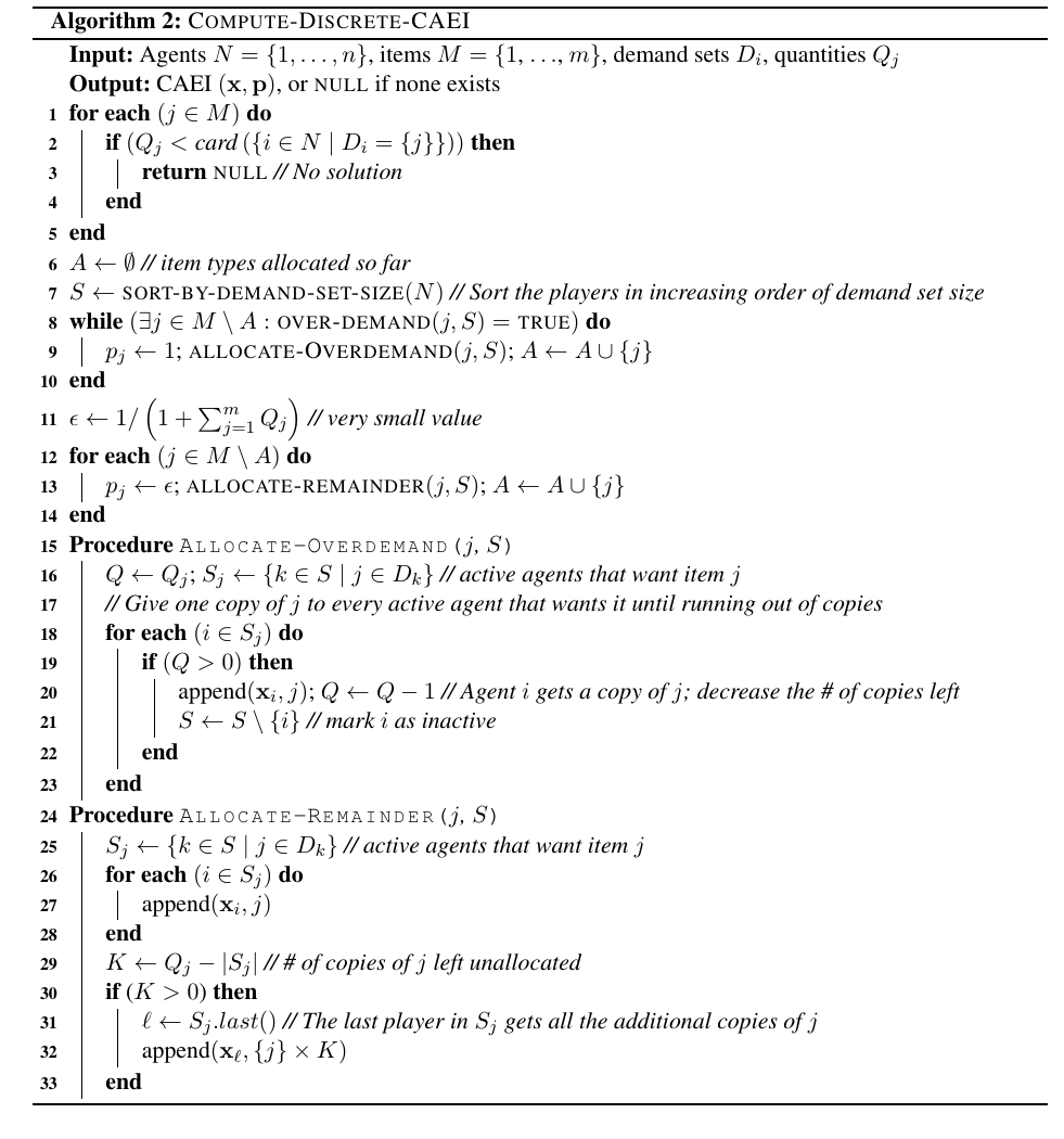
Consider Algorithm 2. Clearly, if there is a set of agents $S$ with singleton demands, such that $D_{i}=\{j\}$ for some $j\in M$ and all $i\in S$, where $|S|>Q_{j}$, then no CAEI can exist. This is because $p_{j}\leq 1$ causes over-demand, and $p_{j}>1$ makes it un-affordable and thereby un-sold.

We claim all other instances admit a CAEI. Algorithm 2 forms a sequence $S$ of active agents, initially containing all the agents sorted in increasing order of $|D_{i}|$, and then iterates over the item types, at each step searching for an item that is desired by more agents among the active ones (i.e. in $S$) than there are copies available. If such an item $j$ is found, then $j$ is allocated at a price of $p_{j}=1$, one copy to each of the first $Q_{j}$ agents in $S$ that want it. All the active agents that got item $j$ are removed from $S$, and the algorithm searches for another such over-demanded and unallocated item among the updated set $S$. Otherwise, when no such item is found, all the goods left are in abundant supply for the agents in $S$ and can be given for a small price ($\epsilon$) among them. Note that these last agents, which are allocated bundles at a price of $\epsilon$ per good, receive not only items that they desire, but in fact all the remaining items.

We argue that the pricing rule ensures that a CAEI is computed. In particular, all the goods are allocated—at latest, the player (or set of players), which receive items in the last round of the algorithm, get all the remaining items. Moreover, the pricing rule is such that each agent $i$ is allocated all of its bundle at once, regardless of whether $\mathbf{x}_{i}$ contains $i$’s required demand set or not. The agents are divided in two categories, namely those who get exactly one item at a price of $1$ (Line 9) and those who get multiple items at a price of $\epsilon$ (Line 13). In both cases, the pricing rule ensures that the allocation $\mathbf{x}_{i}$ costs at most $1$.

Finally, we argue that each agent gets an optimal bundle at the given prices. Let $i$ be an agent that has not received its demand under the allocation $\mathbf{x}$ ($D_{i}\not\subseteq\mathbf{x}_{i}$). The algorithm gives all the agents with singleton demands their required items, so we have $|D_{i}|>1$. We show that agent $i$ cannot afford the set $D_{i}$:

Case 1).

Agent $i$ receives one item priced at $1$. Since all the items have positive prices and $|D_{i}|>1$, we have $\mathbf{p}(D_{i})>1$, so $i$ cannot afford its demand.

Case 2).

Agent $i$ gets an empty bundle. Then agent $i$ never got allocated in the Allocate-Remainder subroutine, which corresponds to the phase where the remaining items are plentiful for the currently unallocated agents. Thus agent $i$ wanted at least one item $j$ allocated in one of the calls to the Allocate-Overdemand subroutine, which means that $p_{j}=1$. From $|D_{i}|>1$, we have $\mathbf{p}(D_{i})>1$ and $i$ cannot afford its demand set.

Case 3).

Agent $i$ receives several items priced at $\epsilon$. If $D_{i}$ contains any item that was allocated at a price of $1$, then clearly buyer $i$ cannot afford $D_{i}$. Otherwise, none of the items in $D_{i}$ was labeled as over-demanded; then buyer $i$ both affords and receives at least one copy of each item in its demand set, which would contradict the choice of agent $i$ as unhappy.

From the case analysis we conclude that each agent $i$ gets an optimal bundle at the current prices, and so $(\mathbf{x},\mathbf{p})$ is a CAEI solution.

The algorithm has at most $m$ rounds, each of which calls the allocate procedure depending on whether there is over-demand or under-demand. In the first type of call, the procedure executes a constant number of operations for each agent in the set of active agents that want the current item, which is clearly bounded by $c\cdot|S|$, where $c$ is a constant and $|S|\leq n$. In the second type of call, of under-demand, the procedure allocates all the players in $S$ one item each, and then gives the last player allocated in that call all the remaining items; this takes $O(n)$ operations. Thus the runtime can be bounded by $poly(m,n,\log{Q_{j}})$.

It follows that in both cases, the algorithm runs in polynomial time, which completes the proof. $\square$

We illustrate the execution of Algorithm 2 through an example.

It is NP-hard to compute a welfare-maximizing CAEI (see, e.g., [8]). However, if we no longer insist that all the items are allocated, we can get a polynomial time algorithm by solving the problem as if the goods were divisible, and then rounding the solution.

We can convert the problem into an instance with divisible goods, where there is one unit from every good and the percentage required by player $i$ from item $j$ is $\frac{D_{i,j}}{Q_{j}}$. Consider the variant of Algorithm 1 where it is not necessary that all the items are sold—note this variant can be obtained with minor modifications, by changing the respective constraints from “$=$” to “$\leq$”. By running such an algorithm, we obtain an optimal allocation from equal incomes with divisible goods without item clearing and which is obtained at some tuple $(\mathbf{x},\mathbf{p})$. Then define a corresponding allocation $\bar{\mathbf{x}}$ in the instance with discrete goods, where $\bar{\mathbf{x}}_{i,j}=\lfloor x_{i,j}\cdot Q_{j}\rfloor$. Then the tuple $(\bar{\mathbf{x}},\mathbf{p})$ satisfies the property that the allocation is feasible, each player gets an optimal bundle at the current prices, and the social welfare is the same as in the corresponding problem with divisible goods. Moreover, no allocation in the problem with discrete goods can obtain higher social welfare than in the corresponding problem with divisible goods. It follows that we obtain a welfare maximizing allocation from equal incomes via Algorithm 1, which runs in time $poly(n,m)$. $\square$

The proof is broken down in three components, corresponding to the scenarios considered. For multiple divisible goods, let there be an instance with $N=\{1,2\}$, $M=\{1,2\}$, and demands $D_{1}=\langle 0.2,0.2\rangle$, $D_{2}=\langle 0.8,0.8\rangle$. Consider the allocation $\mathbf{x}_{1}=\langle 1,0\rangle$, $\mathbf{x}_{2}=\langle 0,1\rangle$. Clearly, this allocation is envy-free since each agent is missing one good in either of the bundles $\mathbf{x}_{1}$, $\mathbf{x}_{2}$. Assume there exist supporting CAEI prices $\mathbf{p}$. By feasability constraints, we have: $p_{1}\leq 1$, $p_{2}\leq 1$ (I). From the optimality condition of CAEI, we must have that no agent can afford a better bundle; in particular, agent $1$ cannot afford their own demand set: $0.2\cdot p_{1}+0.2\cdot p_{2}>1$ (II). From (I) and (II), we have that $5<p_{1}+p_{2}\leq 2$, contradiction.

In the cake cutting model, let $N=\{1,2\}$, $D_{1}=[0,0.4]$, $D_{2}=[0.4,1]$, and consider the envy-free allocation $\mathbf{x}_{1}=[0,0.2]\cup[0.4,0.7]$, $\mathbf{x}_{2}=[0.2,0.4]\cup[0.7,1]$. Suppose there exists a CAEI price curve $\mathbf{p}$ at $\mathbf{x}$; denote by $p_{1},p_{2},p_{3},p_{4}$ the prices of the intervals $[0,0.2]$, $[0.2,0.4]$, $[0.4,0.7]$, $[0.7,1]$, respectively. By feasability constraints, we get: $p_{1}+p_{3}\leq 1$ and $p_{2}+p_{4}\leq 1$ (III). Both agents have a utility of zero at $\mathbf{x}$, so none should afford their demand set, i.e. $p_{1}+p_{2}>1$ and $p_{3}+p_{4}>1$ (IV). From (III) and (IV) we get that $2<p_{1}+p_{2}+p_{3}+p_{4}\leq 2$, contradiction. Thus $\mathbf{p}$ cannot exist.

Finally, for multiple discrete goods, let $N=\{1,2\}$, $M=\{1,2,3,4\}$ with $Q_{j}=1$ $\forall j$, demands $D_{1}=\{1,2\}$, $D_{2}=\{3,4\}$. Consider allocation $\mathbf{x}_{1}=\{1,3\}$, $\mathbf{x}_{2}=\{2,4\}$. Both agents have utilities zero at either bundle $\mathbf{x}_{1},\mathbf{x}_{2}$. The CAEI constraints give: $p_{1}+p_{3}\leq 1$, $p_{2}+p_{4}\leq 1$ (V) and $p_{1}+p_{2}>1$, $p_{3}+p_{4}>1$ (VI). It follows that $2<p_{1}+p_{2}+p_{3}+p_{4}\leq 2$, contradiction.

In all the scenarios considered, the envy-free allocation $\mathbf{x}$ is not a CAEI solution. $\square$

References

- [1] K. J. Arrow, H. Chenery, B. Minhas, and R. Solow. Capital-labor substitution and economic efficiency. The Review of Economics and Statistics, (43(3)):225–250, 1961.
- [2] K. J. Arrow and G. Debreu. Existence of an equilibrium for a competitive economy. Econometrica, (22):265–290, 1954.
- [3] H. Aziz and S. Mackenzie. A discrete and bounded envy-free cake cutting protocol for four agents. In Proceedings of STOC, 2016.
- [4] S. Bouveret and M. Lemaitre. Characterizing conflicts in fair division of indivisible goods using a scale of criteria. In AAMAS, pages 1321–1328, 2014.
- [5] W. Brainard and H. E. Scarf. How to compute equilibrium prices in 1891. In Cowles Foundation Discussion Paper, 2000.
- [6] S. Brams, M. Jones, and C. Klamler. International Journal of Game Theory, 36(3):353–367, 2008.
- [7] S. J. Brams and A. D. Taylor. Fair Division: From Cake-Cutting to Dispute Resolution. Cambridge University Press, 1996.
- [8] S. Branzei, H. Hosseini, and P. B. Miltersen. Characterization and computation of equilibria for indivisible goods. In SAGT, pages 244–255, 2015.
- [9] S. Branzei, A. Procaccia, and J. Zhang. Externalities in cake cutting. In IJCAI, 2013.
- [10] P. Briest, P. Krysta, and B. V ocking. Approximation techniques for utilitarian mechanism design. In STOC, 2005.
- [11] E. Budish. The combinatorial assignment problem: Approximate competitive equilibrium from equal incomes. Journal of Political Economy, 6(119):1061–1103, 2011.
- [12] I. Caragiannis, John K. Lai, and A. D. Procaccia. Towards more expressive cake cutting. In IJCAI, pages 127–132, 2011.
- [13] X. Chen and S. Teng. Spending is not easier than trading: On the computational equivalence of fisher and arrow-debreu equilibria. In ISAAC, pages 647–656, 2009.
- [14] Y. Chevaleyre, P. E. Dunne, U. Endriss, J. Lang, M. Lemaître, N. Maudet, J. Padget, S. Phelps, J. A. Rodríguez-Aguilar, and P. Sousa. Issues in multiagent resource allocation. Informatica, 30:3–31, 2006.
- [15] B. Codenotti and K. R. Varadarajan. Efficient Computation of Equilibrium Prices for Markets with Leontief Utilities. In ICALP, pages 371–382, 2004.
- [16] Y. J. Cohler, J. K. Lai, D. C. Parkes, and A. D. Procaccia. Optimal envy-free cake cutting. pages 626–631, 2011.
- [17] M. Dall’Aglio and F. Maccheroni. Disputed lands. Games and Economic Behavior, 66(1):57–77.
- [18] E. Eisenberg and D. Gale. Consensus of subjective probabilities: The pari-mutuel method. Annals Of Mathematical Statistics, (30):165–168, 1959.
- [19] U. Feige, M. Feldman, N. Immorlica, R. Izsak, B. Lucier, and V. Syrgkanis. A unifying hierarchy of valuations with complements and substitutes. In AAAI, pages 872–878, 2015.
- [20] Michal Feldman and Brendan Lucier. Clearing markets via bundles. In SAGT, pages 158–169, 2014.
- [21] D. Foley. Resource allocation and the public sector. Yale Econ. Essays, 7:45–98, 1967.
- [22] A. Ghodsi, M. Zaharia, B. Hindman, A. Konwinski, S. Shenker, and I. Stoica. Dominant resource fairness: Fair allocation of multiple resource types. In NSDI, pages 323–336, 2011.
- [23] J. Goldman and A. D. Procaccia. Spliddit: Unleashing fair division algorithms. SIGecom Exchanges, 13(2):41–46, 2014.
- [24] F. Husseinov and N. Sagara. Existence of efficient envy-free allocations of a heterogeneous divisible commodity with nonadditive utilities. Social Choice and Welfare, 41(4), pages = 923-940).
- [25] J. Kleinberg and E. Tardos. Algorithm Design. Pearson, 2005.
- [26] D. Kurokawa, J. K. Lai, and A D. Procaccia. How to cut a cake before the party ends. In AAAI, 2013.
- [27] J. O. Ledyard. Optimal combinatoric auctions with single-minded bidders. In EC, pages 237–242, 2007.
- [28] R. Maxfield. General equilibrium and the theory of directed graphs. Journal of Mathematical Economics, 27(1):23–51, 1997.
- [29] R. Mehta and M. Sohoni. Exchange markets: Strategy meets supply-awareness - (abstract). In WINE, pages 361–362, 2013.
- [30] H. Moulin. Fair Division and Collective Welfare. MIT Press, 2004.
- [31] N. Nisan, T. Roughgarden, E. Tardos, and V. Vazirani (Eds.). Algorithmic Game Theory. Cambridge University Press, 2007.
- [32] A. Othman, C. H. Papadimitriou, and A. Rubinstein. The complexity of fairness through equilibrium. In ACM-EC, pages 209–226, 2014.
- [33] A. D. Procaccia. Cake cutting: Not just child’s play. CACM, 56(7):78–87, 2013.
- [34] A. D. Procaccia. Cake cutting algorithms, 2014. Draft of Chapter 13 of the Handbook of Computational Social Choice.
- [35] J. M. Robertson and W. A. Webb. Cake Cutting Algorithms: Be Fair If You Can. A. K. Peters, 1998.
- [36] V. Robu, D. Parkes, T. Ito, and N. R. Jennings. Efficient interdependent value combinatorial auctions with single minded bidders. In IJCAI, 2013.
- [37] E. Segal-Halevi, A. Hassidim, and Y. Aumann. Envy-free cake-cutting in two dimensions. In AAAI, pages 1021–1028, 2015.
- [38] E. Segal-Halevi, S. Nitzan, A. Hassidim, and Y. Aumann. Fair and square: Cake-cutting in two dimensions. CoRR, abs/1510.03170, 2015.
- [39] Erel Segal-Halevi, Avinatan Hassidim, and Yonatan Aumann. Waste makes haste: Bounded time protocols for envy-free cake cutting with free disposal. In Proceedings of AAMAS, pages 901–908, 2015.
- [40] R.M. Solow. A contribution to the theory of economic growth. The Quarterly Journal of Economics, (70):65–94, 1956.
- [41] H. Steinhaus. Mathematical Snapshots. Oxford, 1951. second edition.
- [42] H. Varian. Equity, envy and efficiency. Journal of Econ. Theory, 9:63–91, 1974.
Appendix A Missing Proofs
Theorem 11
Given a fair division instance with single minded valuations and divisible goods, and allocation , a CAEI solution at can be found in polynomial time (if one exists). Similarly, given price vector a matching allocation can be found in polynomial time.
Proof:
Given , let be the set of agents that can afford their demand at these prices; that is, for each , we have that . Then an equilibrium allocation can be found by solving the following constraints with variable :
That is, we require that each agent can afford its own bundle, the agents in get their demand set, all the goods are allocated and the allocation is feasible.
For the second part of the theorem, suppose we are given an allocation . Let be the set of agents that receive their demand under , i.e. for which . If satisfies basic feasability constraints (i.e. all the items are sold and ), Then a price vector that matches the allocation (if it exists) can be found by solving the following linear program: