Under review–do not distribute. Contact the authors before citing.
A Day of Your Days: Estimating Individual Daily Journeys Using Mobile Data to Understand Urban Flow
Abstract
Nowadays, travel surveys provide rich information about urban mobility and commuting patterns. But, at the same time, they have drawbacks: they are static pictures of a dynamic phenomena, are expensive to make, and take prolonged periods of time to finish. However, the availability of mobile usage data (Call Detail Records) makes the study of urban mobility possible at levels not known before. This has been done in the past with good results–mobile data makes possible to find and understand aggregated mobility patterns. In this paper, we propose to analyze mobile data at individual level by estimating daily journeys, and use those journeys to build Origin-Destiny matrices to understand urban flow. We evaluate this approach with large anonymized CDRs from Santiago, Chile, and find that our method has a high correlation () with the current travel survey, and that it captures external anomalies in daily travel patterns, making our method suitable for inclusion into urban computing applications.
1 Introduction
Travel surveys provide information about urban mobility and commuting patterns, mainly through Origin-Destiny matrices derived from them. These matrices allow urban planners and policy makers to understand travel patterns in urban mobility. Such surveys are usually collected once per decade, due to their expensiveness (both in time and monetary costs). Moreover, they are limited in some ways: travel surveys are static pictures of a dynamic phenomena and, due to its sample size, they are limited to big areas (either administrative or designed).
In this paper, we propose to use mobile data used for billing, which indicates a subset of the antennas a mobile device has connected through the day, as well as the corresponding timestamps. We use these digital footprints to build extended travel diaries. Travel diaries are the basic elements of travel surveys, but we extend them through daily journeys, as we detect not only trips, but also other “non-trip” activities. From these daily journeys we build Origin-Destiny (OD) matrices, at a fraction of the expenses needed to build OD matrices from travel surveys.
Our main contribution is a method to detect these disaggregated daily journeys using Call Detail Records (CDRs). Our approach is based on graphical timelines and computational geometry algorithms, which are applied having in mind transport-based rules regarding trip duration and distance. We use an anonymized CDR dataset from one of the largest telecommunications company in Chile, with a market share of 38.18% as of June 2015. Chile, being one of the developing countries with highest mobile phone penetration, is a good candidate for analyzing urban mobility using CDRs--for instance, there are 132 mobile subscriptions per 100 inhabitants.11 1 http://www.subtel.gob.cl/estudios-y-estadisticas/telefonia/ Particularly, we focus on Santiago, its capital and most populated city.
To evaluate our results, we compare our predicted urban flow (in the form of an OD matrix) with the last travel survey for Santiago, performed during 2012–2013. In terms of OD pairs, we obtain a very high correlation (), indicating that our method recognizes the urban flow on the city. We apply our methods at different days, and find that, in addition, we detect how urban flows change in the presence of unexpected conditions. This, jointly with the disaggregated nature of our method, has potential for applications in urban computing [13], discussed at the end of this paper.
2 Related Work
The estimation of OD matrices, and thus, urban mobility patterns, is not new. The most basic way of estimating those patterns is by travel surveys, but also other methods have been developed. A common method is based on traffic counts [2], but the massive availability of other kinds of information has allowed to estimate such matrices in other ways, for instance, by using smart-card passive data [9] and, as in this paper, mobile data [5, 11, 1, 7, 4].

The work on mobile datasets has included both theory and practice. From a theoretical point of view, the analysis of how predictable humans are [5, 11]. A practical work has been the prediction of transient OD matrices by analyzing transitions of connections between cell antennas. These transitions are the basis of many methods, which employ techniques from optimization and temporal association rules [4], to transport-based rules to accept or discard transitions [7, 1]. Our approach is also based on antenna transitions. However, the main difference with previous work is that we reconstruct individual daily journeys, an extended version of the travel diaries used to build travel surveys. These journeys are built using a geometric approach based on graphical timelines [12], which are time-space diagrams displaying timelines according to time and distance covered. On these timelines we estimate the “turning points” of the daily journey, which serve to differentiate daily activities into trips and non-trips. These timetables are regularly used in transport to display and analyze schedules, as well as phenomena associated with vehicle behavior. For instance, Figure 1 shows a train schedule designed in 1885 by Étienne-Jules Marey. On it, passengers can see arrival and departure times, as well as the duration of stops and the velocity of trains. Transport planners can study vehicle behavior–since all vehicles share the same origin, if we were visualizing their true trajectories instead of the scheduled ones, vehicle bunching can be recognized immediately [8].
3 Methods
Our methods consider mobile user traces estimated from anonymized CDR data. CDRs are comprised of logged data extracted from cell-phone antennas, and are used to bill customers. They contain the following events: calls, SMS (text messages), and data events (triggered every 15 Megabytes or every 15 minutes of an active connection). The following features are common between all events, and thus are considered for analysis: the anonymized user ID, the antenna ID, and time of the day. The antenna ID is used to determine a likely position for the user at the corresponding time of the day. Note that this position is assumed to be the same for all phones connected to the same antenna, i. e., we do not perform triangulation based on signal strength with nearby antennas.
Problem Definition and Proposal. The problem we propose to solve is the estimation of a diary of activities for a day, using CDRs from mobile data. A daily journey for user is defined as follows:
Where is an activity, (and ) are the positions (and times) associated to the start/origin and end/destination of . Activities can be of types trip, non-trip, and unknown.
To solve this problem we propose a two-step algorithm: first, we define the candidate turning points of a day, where turning point is a moment in the day, at a specific position, where the user started to perform an activity (and, by definition, ends performing a previous activity). The second step is to detect activities based on the candidate turning points.
Graphical Timetables and Turning Points. For all users, we build the following vector:
Where each element in corresponds to an event in the CDR events of in a day, with the corresponding timestamp and the antenna position . These vectors can be transformed into graphical timetables (see Figure 1), where the x-axis is the elapsed time during the day, and the y-axis is the traveled (accumulated) distance from the starting point. The different groups of segments present in the timetable define the activities in .

However, due to the potential amount of CDR events, several contiguous segments could be related to the same activity. To tackle this, we propose to simplify the timetable using the Ramer-Douglas-Pecker line simplification algorithm [3]. This algorithm, depicted on Figure 2, starts with the extremes of the trajectory, and iteratively adds vertices according to their distance to the candidate simplified line. The vertex with greater distance (or error) is added, and the process is repeated until the error is less than a given tolerance. This results in a simplified vector , which contains candidate “turning points” of daily activity. Those candidate points define the potential activity segments that will end defining .
Activity Classification. The second step is to identify which contiguous segments in the line defined by the points of can be merged into a single activity . The most direct approach is to merge a series of horizontal (or nearly horizontal) segments. However, a continuously moving user (and thus, with non-horizontal segments) is also feasible. Take the example of a taxi driver, whose primary activity during the day is working as a driver. Although these activities are valid, they are not relevant for an OD matrix, as they are not trips in the individual sense. Thus, we define the following classifications: unknown, non-trips, and trips.
Unknown are segments where the total distance covered is greater than 100 kilometers. In those cases we cannot distinguish between trips and unknown situations. For instance, the mobile number is associated to a vehicle (e. g., a taxi) or another vehicle/device. While these are indeed displacements in time and space, they do not fall on the daily journey concept we study in this paper. Another case is when users switch to WiFi networks, and thus disappear from the event log for a long period of time. For instance, users who switch to the wireless network of their work place might not be detected there, and the next logged event could appear after working hours. On those cases, we cannot identify trips reliably. To avoid this scenario, in some cases the displacement between events has been limited to specific time windows (e. g., 10 minutes and 1 hour [7]).
Non-trips are segments that are not unknown. The criteria to assign this type to an activity is based on the covered distance and time. On the one hand, the antenna density of origin/destiny locations of the activity is considered to determine a minimum distance that cannot be attributed to signalling changes (this is discussed further in the next section). On the other hand, some activities involve displacements (e. g., working/studying in a big campus), but the speed of movement is much slower than when performing a trip. Thus, if there is a distance displacement, but the time is greater than 180 minutes, we still consider a non-trip activity.
Finally, trips are segments that are not unknown and are not non-trip, but, in addition to the 180 minute rule, we enforce a minimum duration of 15 minutes for a segment, due to the granularity of the CDR data. Any other activity that does not fall into the rules defined above is considered is considered unknown.
Activity Merging. Having assigned an activity to each segment built from , we procede to merge contiguous segments that have the same activity. Two or more segments are merged into an activity by considering the first time and position in the segment as origin, and the last time and position in the segment as destination. We also consider an additional case: when two trip activities surround a non-trip activity, and the duration of the latter is lesser or equal than 15 minutes, its activity is changed to trip. This scenario correspond to situations when users in public transport make a connection, or users in vehicles face congested traffic. In this way, after merging all activities, the daily journey is built.
4 Context and Dataset

We work with a dataset from Santiago, the capital of Chile. Santiago is a city with almost 8 million inhabitants, and it has an integrated public transport system named Transantiago. The Metropolitan Area of Santiago is composed of 35 independent administrative units named municipalities. We work with this set of municipalities, depicted on Figure 3.
Santiago 2012 Travel (OD) Survey. The Santiago 2012 travel survey (ODS hereafter) was performed during 2012--2013.22 2 http://www.sectra.gob.cl/biblioteca/detalle1.asp?mfn=3253. It took almost one year to finish, and contains 96,013 trips (from 40,889 users). The information of trips is obtained through the travel diaries fulfilled by the surveyed persons. The ODS, used to define public policy related to public and private transport in the city, as well as general urban mobility, is performed every 10 years due to its costs and its difficulty.
The survey considers other municipalities outside the area, as well as cities in other regions, due to the characteristics of the survey procedure. Additionally, the survey also defines a zoning of the city, with 752 zones within the considered municipalities. Each zone intends to control for land-use and population density. Even though each trip in the survey is associated to a zone and a municipality, the survey is only representative at municipal level. At its current granularity, the data available is not enough to calculate reliable mobility patterns at zone level.
In this paper, without losing generality, we focus on the 51,819 trips performed on working days, from 22,541 users, performed on the inner 35 municipalities of the Metropolitan Area. We aggregated trips according to municipality into an OD matrix, shown in Figure 4. One can see that the most common trips are intra-municipalities, but there are still municipalities that tend to receive more trips than others. This is because most of the commercial and working land-use is on the municipalities of Santiago, Providencia, Las Condes and Vitacura. Note that the municipality of Santiago is at the center of the Santiago Metropolitan Area. In the rest of this paper, when we mention Santiago we refer to the Metropolitan Area.

In terms of trip variables, Figure 5 shows the distributions of trip start time, trip duration, and approximated trip distance (i. e., euclidean distance). One can see that trip start time follows an expected pattern of two high peaks (one in the morning and one in the afternoon), with a third smaller peak at lunch time. With respect to trip duration, the mean duration is 41 minutes. Note that the self-reported nature of the survey is evident, due to the several peaks present on the distribution in 15 minute periods (e. g., 30 and 45 minutes). Finally, with respect to travel distance, the mean euclidean distance is 6.05 kilometers.

Mobility Data. We analyze mobile data using CDRs from one of the
largest telecommunications company in Chile. The CDR data contains
events for all Mondays and Tuesdays of June 2015.
In the 35
municipalities under consideration, the company has 12,936 antennas,
with 98% of the zones having at least one antenna. Figure
6 displays the antenna territorial
density. Note that the antenna distribution is not homogeneous on the
city, nor at any level. For instance, antenna distribution is correlated
with the ODS, considering aggregated destinations at municipal level
(, ).

To avoid artifacts in the trip detection introduced by connectivity changes due to signal strength (i. e., mobile phones looking for the best signal) and signal balancing (i. e., mobile antennas pointing devices to connect to other antennas due to saturation), we estimated a distance matrix for all antennas in each zone. Then, we defined that the minimum distance for an activity to be considered a trip between zones and is:
Where is the quantile function (by manual experimentation we have found that is a good value). The mean value of is 732 meters (minimum of 45 m., and maximum of 14.1 km.).
While we do not disclose the exact number of users in each day due to confidentiality and commercial issues, Figure 7 displays the distributions of event frequency and hourly entropy for all days in the dataset. In the left chart, each dot is a minute in a specific day. The frequency encodes the fraction of events that the dot contains per day. One can see that the distribution of frequency of events can be approximated by a cubic linear regression, with a higher frequency of events in the afternoon.
The right chart of Figure 7 displays the distribution of user entropy with respect to hours of the day, for each day. This entropy is defined as the Shannon entropy of user :
Where is the probability that user has a CDR event in the th hour of the day. The purpose of estimating this entropy is to have a measure of diversity with respect to time for each user. Thus, we discard users who do not have enough diversity to be able to estimate their journeys, or that have too much diversity to be normal users (e. g., they could be SIM cards associated to machines). We discarded users in the first quartile () and in the last decile ().

We apply our methods to this dataset on the following section. To be able to compare with the ODS, we employ a similar sample size of randomly selected mobile users (before filtering by entropy).
5 Daily Journeys and OD Matrix
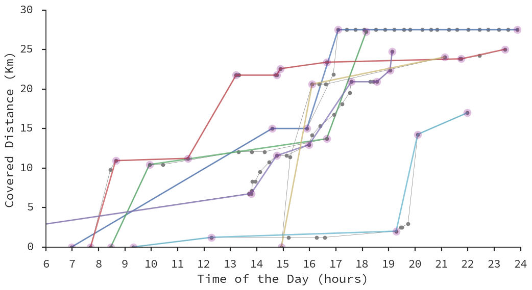
We applied our method to generate daily journeys to the CDR dataset. Figure 8 shows the result of randomly selected samples from the dataset. Each colored line is a different user, and the grey line underneath each colored line is the original timetable before simplification. The remaining “turning points” are rendered in purple, with a bigger size for easy identification on the image. Those points define the activity segments which we classify as unknown, non-trip and trip according to the definitions provided earlier.
| Date | N | # Trips | Mean Time (m) | Mean Distance (km) |
|---|---|---|---|---|
| 2015-06-01 | 37,037 | 56,148 | 78.38 | 7.68 |
| 2015-06-02 | 37,622 | 57,764 | 77.78 | 7.74 |
| 2015-06-08 | 34,272 | 50,017 | 83.86 | 7.80 |
| 2015-06-09 | 34,611 | 50,778 | 83.03 | 7.77 |
| 2015-06-15 | 36,274 | 53,642 | 79.45 | 7.68 |
| 2015-06-16 | 36,804 | 56,046 | 78.16 | 7.68 |
| 2015-06-22 | 34,288 | 49,434 | 80.05 | 7.78 |
| 2015-06-23 | 36,239 | 54,983 | 77.62 | 7.71 |
| 2015-06-29 | 22,770 | 31,963 | 74.78 | 7.50 |
| 2015-06-30 | 35,181 | 52,597 | 78.94 | 7.66 |
After estimating the daily journeys from the graphical timetables, we discarded users without trip and non-trip activities. Table 1 shows the final number of users considered (after filtering by entropy, and after filtering without valid trips/non-trips). From these activities, we built a transient OD matrix for each day, using the initial and final positions of each trip, which were assigned to their corresponding municipalities. Since we estimated matrices for many days, we averaged the number of trips for each OD pair of origin/destiny municipalities . Figure 9 shows the resulting matrix.

We also estimated the trip variables analyzed before for the ODS. Figure 10 shows the kernel density estimations of each distribution for each day. One can see that, overall, the distributions are mostly similar for all days, with the following exceptions: start time distribution is different on June 29th, and trip duration distribution is different on June 8th and 9th. On June 9th there was a strike in the Santiago public transport system, which explains partly the increased trip time in comparison to the other days. Additionally, on June 29th the semi-final of the latin-american soccer championship Copa América, where Chile was a contender, was played at 8pm. One can see that the number of trips in the afternoon was much higher than in the morning, making the morning peak to shrink in the density estimation. Moreover, the distribution highlights that the afternoon peak was earlier than usual, and that there was a night peak after the soccer match.

Table 1 shows the number of users (and their trips), the mean trip duration, and the mean euclidean distance of trips for each day. Mean times vary within 74.78 and 83.86 minutes, and mean distances vary within 7.5 and 7.8 kilometers. One can see that both distance and time are over-estimated in comparison to the ODS (mean time 41 minutes; and mean distance 6.05 kilometers). The differences in time could appear due to the latency in antenna changes and to CDR event granularity (which happens every 15 minutes in the case of data connections). The differences in distance could be explained by the approximation of each individual position to the corresponding antennas. However, even though the means are different, the distributions have similar shapes to those from the ODS, as displayed on Figure 10.
Comparisons with ODS. A key question is how much different our results are with respect to the ODS. First, we estimated the Spearman rank-correlation between our results and the ODS at municipal level, obtaining (). The correlation is very high, which means that our averaged matrix reflects the flow of people in the city very well. To compare to what extent our result is good, we refer to a 2013 OD matrix estimated from the public transport smart-card data [9].33 3 http://www.dtpm.cl/index.php/2013-04-29-20-33-57/matrices-de-viaje This matrix has a correlation of () with the ODS, a result that indicates that the ODS captures a diversity of trip modes, not only public transport. We also tested what happened if we did not consider the matrix diagonal (i. e., without intra-municipal trips), and we observed that we mantain our correlation, while the public transport OD increased (). This makes sense–short trips are less likely to use public transport (e. g., if the destiny is at walking distance).

Finally, we visually compare whether the distributions of start time, trip duration and trip distance are similar to those of the ODS. To do, Figure 12 shows the Cumulative Density Functions of these variables. We observe that, in terms of start time and euclidean distance, the CDFs are very similar, although in terms of trip duration there is a noticeable difference, as mentioned earlier.

6 Discussion and Conclusions
In this paper we predicted OD matrices from daily journeys built using mobile data. We did so by proposing a geometric approach based on graphical timelines, and found that, using a sample from mobile data connectivity, we were able to reconstruct the OD pairs in a city, at municipal level, with a very high correlation. Moreover, we were able to estimate start time, trip time and trip distance, in a way that resembled the ODS results, with exception of trip time, which needs calibration to account for the delay in antenna change with respect to the moment in which each trip started.
Implications. On the one hand, our algorithm is very simple and can work with streaming data if what matters is the number of trips. Consider the day in which a soccer match was played, and peak hours shifted. Reportedly, the transport authorities did not account for this shift, and instead they only created ad-hoc routes in public transport.44 4 http://www.mtt.gob.cl/copaamerica/santiago. Thus, our results could support urban computing applications [13] which need almost real-time transport data. On the other hand, our method complements the ODS in important ways. The ODS is performed every 10 years, but, as with any static picture, it does not capture rich context-dependant dynamics of the city. Conversely, our approach is more dense, as it can be applied even at daily scale to observe differences that the ODS does not. In this paper we have shown that, even working with a sample of anonymous data from mobile data, it is possible to reconstruct part of the ODS, as well as finding diverging days from the typical patterns, at a fraction of its costs. This can be used to measure, for instance, what are the effects in urban flows caused by transport measures like road space rationing.
Limitations and Future Work. Our geometric algorithm, with arguably reasonable transport-based constraints, does not consider information that could be useful in determining the turning points of the day (e. g., land-use or census information). Additionally, the distance and time estimation need to be corrected using scaling factors. Then, in addition to address our limitations, the main line of research for future work will be the characterization of non-trip activities. One way of performing such characterization is through the analysis of land-use derived from mobile data analysis [6, 10].
Acknowledgements. We thank Oscar Peredo, José García and Pablo García for valuable discussion.
References
- [1] Lauren Alexander, Shan Jiang, Mikel Murga and Marta˜C Gonz\’alez “Origin–destination trips by purpose and time of day inferred from mobile phone data” In Transportation Research Part C: Emerging Technologies Elsevier, 2015
- [2] Ennio Cascetta “Estimation of trip matrices from traffic counts and survey data: a generalized least squares estimator” In Transportation Research Part B: Methodological 18.4 Elsevier, 1984, pp. 289–299
- [3] David˜H Douglas and Thomas˜K Peucker “Algorithms for the reduction of the number of points required to represent a digitized line or its caricature” In Cartographica: The International Journal for Geographic Information and Geovisualization 10.2 University of Toronto Press, 1973, pp. 112–122
- [4] Vanessa Frias-Martinez, Cristina Soguero and Enrique Frias-Martinez “Estimation of urban commuting patterns using cellphone network data” In Proceedings of the ACM SIGKDD International Workshop on Urban Computing, 2012, pp. 9–16 ACM
- [5] Marta˜C Gonzalez, Cesar˜A Hidalgo and Albert-Laszlo Barabasi “Understanding individual human mobility patterns” In Nature 453.7196 Nature Publishing Group, 2008, pp. 779–782
- [6] Eduardo Graells-Garrido and Jos\’e Garc\’ia “Visual Exploration of Urban Dynamics Using Mobile Data” In Proceedings of Ubiquitous Computing and Ambient Intelligence. Sensing, Processing, and Using Environmental Information: 9th International Conference, UCAmI 2015, 2015, pp. 480–491 Springer International Publishing
- [7] Md˜Shahadat Iqbal, Charisma˜F Choudhury, Pu Wang and Marta˜C Gonz\’alez “Development of origin–destination matrices using mobile phone call data” In Transportation Research Part C: Emerging Technologies 40 Elsevier, 2014, pp. 63–74
- [8] Lu\’s Moreira-Matias, Carlos Ferreira, Jo\˜ao Gama, Jo\˜ao Mendes-Moreira and Jorge˜Freire Sousa “Bus bunching detection by mining sequences of headway deviations” In Advances in Data Mining. Applications and Theoretical Aspects Springer, 2012, pp. 77–91
- [9] Marcela˜A Munizaga and Carolina Palma “Estimation of a disaggregate multimodal public transport Origin–Destination matrix from passive smartcard data from Santiago, Chile” In Transportation Research Part C: Emerging Technologies 24 Elsevier, 2012, pp. 9–18
- [10] Kentaro Nishi, Kota Tsubouchi and Masamichi Shimosaka “Extracting land-use patterns using location data from smartphones” In Proceedings of the First International Conference on IoT in Urban Space, 2014, pp. 38–43 ICST (Institute for Computer Sciences, Social-InformaticsTelecommunications Engineering)
- [11] Chaoming Song, Zehui Qu, Nicholas Blumm and Albert-L\’aszl\’o Barab\’asi “Limits of predictability in human mobility” In Science 327.5968 American Association for the Advancement of Science, 2010, pp. 1018–1021
- [12] Edward˜R Tufte “Envisioning information” Graphics Press, 1993
- [13] Yu Zheng, Licia Capra, Ouri Wolfson and Hai Yang “Urban computing: concepts, methodologies, and applications” In ACM Transactions on Intelligent Systems and Technology (TIST) 5.3 ACM, 2014, pp. 38