A Discrete Divergence Free Weak Galerkin Finite Element method for the Stokes Equations

The Stokes problem seeks unknown functions ${\bf u}$ and $p$ satisfying

where $\Omega$ is a polygonal domain in $\mathbb{R}^{d}$ with $d=2,3$ and $A$ is a symmetric and positive definite $d\times d$ matrix-valued function in $\Omega$. For the nonhomogeneous boundary condition

one can use the standard procedure by letting ${\bf u}={\bf u}_{0}+{\bf u}_{g}$. ${\bf u}_{g}$ is a known function satisfying ${\bf u}_{g}={\bf g}$ on $\partial\Omega$ and ${\bf u}_{0}$ is zero at $\partial\Omega$ and satisfies (1)-(2) with different right hand sides.

The weak form in the primary velocity-pressure formulation for the Stokes problem (1)–(3) seeks ${\bf u}\in[H_{0}^{1}(\Omega)]^{d}$ and $p\in L_{0}^{2}(\Omega)$ satisfying

In the standard finite element methods for the Stokes and the Navier-Stokes equations, both pressure and velocity are approximated simultaneously. The primitive system is a large saddle point problem. Numerical solvers for such indefinite systems are usually less effective and robust than solvers for definite systems. On the other hand, the divergence-free finite element method, discrete or exact, computes numerical solution of velocity by solving a symmetric positive definite system in a divergence-free subspace. It eliminates the pressure from the coupled equations and hence significantly reduces the size of the system. The divergence-free method is particularly attractive in the cases where the velocity is the primary variable of interest, for example, the groundwater flow calculation. The main tasks in the implementation of the divergence-free method are to understand divergence-free subspaces, weakly or exactly, and to construct bases for them.

Many finite element methods, continuous [2, 3, 8] and discontinuous [1, 4, 11, 12, 16], have been developed and analyzed for the Stokes and the Navier-Stokes equations. Divergence-free basis for different finite element methods have been constructed [5, 6, 7, 9, 10, 17, 18, 19].

A weak Galerkin finite element method was introduced in [15] for the Stokes equations in the primal velocity-pressure formulation. This method is designed by using discontinuous piecewise polynomials on finite element partitions with arbitrary shape of polygons/polyhedra. Weak Galerkin methods were first introduced in [13, 14] for second order elliptic equations. In general, weak Galerkin finite element formulations for partial differential equations can be derived naturally by replacing usual derivatives by weakly-defined derivatives in the corresponding variational forms, with an option of adding a stabilization term to enforce a weak continuity of the approximating functions. Therefore the weak Galerkin method developed in [15] for the Stokes equations naturally has the form: find ${\bf u}_{h}\in V_{h}$ and $p_{h}\in W_{h}$ satisfying

for all the test functions ${\bf v}\in V_{h}$ and $q\in W_{h}$ where $V_{h}$ and $W_{h}$ will be defined later. The stabilizer $s({\bf u}_{h},{\bf v})$ in (6) is parameter independent.

Let $D_{h}$ be a discrete divergence free subspace of $V_{h}$ such that $(\nabla_{w}\cdot{\bf v},q)=0$ for ant $q\in W_{h}$. Then the discrete divergence free WG formulation is to find ${\bf u}_{h}\in D_{h}$ satisfying

System (8) is symmetric and positive definite with many fewer unknowns. The main purpose of this paper is to construct bases for $D_{h}$ in two and three dimensional spaces. A unique feature of these divergence free basis functions is that they can be obtained on general meshes such as hybrid meshes or meshes with hanging nodes. Numerical examples in two dimensional space are provided to confirm the theory. Although the Stokes equations is considered, the divergence free basis can be use for solving the Navier-Stokes equations.

In this section, we will review the WG method for the Stokes equations introduced in [15] with $k=1$.

Let ${\cal T}_{h}$ be a partition of the domain $\Omega$ consisting mix of polygons satisfying a set of conditions specified in [14]. In addition, we assume that all the elements $T\in{\mathcal{T}}_{h}$ are convex. Denote by ${\cal F}_{h}$ the set of all edges in 2D or faces in 3D in ${\cal T}_{h}$, and let ${\cal F}_{h}^{0}={\cal F}_{h}\backslash\partial\Omega$ be the set of all interior edges or faces.

We define a weak Galerkin finite element space for the velocity as follows

We would like to emphasize that there is only a single value ${\bf v}_{b}$ defined on each edge in 2D and face in 3D. For the pressure variable, we have the following finite element space

For a given ${\bf v}\in V_{h}$, a weak gradient and a weak divergence are defined locally on each $T\in{\mathcal{T}}_{h}$ as follows.

Denote by $Q_{0}$ the $L^{2}$ projection operator from $[L^{2}(T)]^{d}$ onto $[P_{1}(T)]^{d}$ and denote by $Q_{b}$ the $L^{2}$ projection from $[L^{2}(e)]^{d}$ onto $[P_{0}(e)]^{d}$. Let $({\bf u};p)$ be the solution of (1)-(3). Define $Q_{h}{\bf u}=\{Q_{0}{\bf u},Q_{b}{\bf u}\}\in V_{h}$. let $\mathbb{Q}_{h}$ be the local $L^{2}$ projections onto $P_{0}(T)$.

We introduce three bilinear forms as follows

Define

The following optimal error estimates have been derived in [15].

Define a discrete divergence free subspace $D_{h}$ of $V_{h}$ by

By taking the test functions from $D_{h}$, the weak Galerkin formulation (11)-(12) is equivalent to the following divergence-free weak Galerkin finite element scheme.

System (17) is symmetric and positive definite with many fewer unknowns. It can be solved effectively by many existing solvers.

The main task of this paper is to construct basis for $D_{h}$. In the next two sections, discrete divergence free bases will be constructed explicitly for two and three dimensional spaces.

For a given partition ${\mathcal{T}}_{h}$, let ${\cal V}_{h}^{0}$ be the set of all interior vertices. Let $N_{F}=card({\mathcal{F}}_{h}^{0})$, $N_{V}=card({\cal V}_{h}^{0})$ and $N_{K}=card({\mathcal{T}}_{h})$. It is known based on the Euler formula that for a partition consisting of convex polygons, then

For a mesh ${\mathcal{T}}_{h}$ with hanging nodes, the relation in (18) is still true if we treat the hanging nodes as vertices.

First we need to derive a basis for $V_{h}$. For each $T\in{\mathcal{T}}_{h}$ and any ${\bf v}=\{{\bf v}_{0},{\bf v}_{b}\}\in V_{h}$, ${\bf v}_{0}$ is a vector function with two components and each component is a linear function. Therefore there are six linearly independent linear functions $\Phi_{j+1},\Phi_{j+2},\cdots,\Phi_{j+6}$ in $V_{h}$ such that they are nonzero only at the interior of element $T$. For each $e_{i}\in{\mathcal{F}}_{h}^{0}$, ${\bf v}_{b}$ is a constant vector function. Thus, there are two linearly independent constant functions $\Psi_{i,1}$ and $\Psi_{i,2}$ in $V_{h}$ which take nonzero value only on $e_{i}$. Then it is easy to see that

For a given function ${\bf v}=\{{\bf v}_{0},{\bf v}_{b}\}\in V_{h}$, it is easy to see that ${\bf v}_{0}$ can be spanned by the basis functions $\Phi_{i}$ and ${\bf v}_{b}$ by the basis functions $\Psi_{j,k}$.

Next, we will find the dimension of $D_{h}$. Since the dimension for pressure space $W_{h}$ is $N_{K}-1$, it follows from (18) that

For any $e_{i}\in{\mathcal{F}}_{h}^{0}$,let $\psi_{i,1}$ and $\psi_{i,2}$ be two basis functions of $V_{h}$ associated with $e_{i}$. Let ${\bf n}_{e_{i}}$ and ${\bf t}_{e_{i}}$ be a normal vector and a tangential vector to $e_{i}$ respectively. Define $\Upsilon_{i}=C_{1}\Psi_{i,1}+C_{2}\Psi_{i,2}$ such that $\Upsilon_{i}|_{e_{i}}={\bf t}_{e_{i}}$. Obviously $\Upsilon_{i}\in V_{h}$ is only nonzero on $e_{i}$.

For a given interior vertex $P_{i}\in{\cal V}_{h}^{0}$, assume that there are $r$ elements having $P_{i}$ as a vertex which form a hull ${\cal H}_{P_{i}}$ as shown in Figure 1. Then there are $r$ interior edges $e_{j}$ ($j=1,\cdots,r$) associated with ${\cal H}_{P_{i}}$. Let ${\bf n}_{{e_{j}}}$ be a normal vector on $e_{j}$ such that normal vectors ${\bf n}_{e_{j}}$ $j=1,\cdots,r$ are counterclockwise around vertex $P_{i}$ as shown in Figure 1. For each $e_{j}$, let $\Psi_{j,1}$ and $\Psi_{j,2}$ be the two basis functions of $V_{h}$ which is only nonzero on $e_{j}$. Define $\Theta_{j}=C_{1}\Psi_{j,1}+C_{2}\Psi_{j,2}\in V_{h}$ such that $\Theta_{j}|_{e_{j}}={\bf n}_{e_{j}}$. Define $\Lambda_{i}=\sum_{j=1}^{r}\frac{1}{|e_{j}|}\Theta_{j}$.

Let ${\mathcal{T}}_{h}$ be a partition of $\Omega\subset\mathbb{R}^{3}$ consisting polyhedrons without hanging nodes. Recall $N_{F}=card({\mathcal{F}}_{h}^{0})$, $N_{V}=card({\cal V}_{h}^{0})$ and $N_{K}=card({\mathcal{T}}_{h})$. Denote by ${\mathcal{E}}_{h}$ all the edges in ${\mathcal{T}}_{h}$ and let ${\mathcal{E}}_{h}^{0}={\cal E}_{h}\backslash\partial\Omega$. Let $N_{E}=card({\mathcal{E}}_{h}^{0})$.

It is known based on the Euler formula that for a partition consisting of convex polyhedrons, then

For each $T\in{\mathcal{T}}_{h}$ and any ${\bf v}=\{{\bf v}_{0},{\bf v}_{b}\}\in V_{h}$, ${\bf v}_{0}$ is a vector function with three components and each component is a linear function. Therefore there are twelve linearly independent linear functions $\Phi_{j+1},\Phi_{j+2},\cdots,\Phi_{j+12}$ in $V_{h}$ such that they are nonzero only at the interior of element $T$. For each face $f_{i}\in{\mathcal{F}}_{h}^{0}$, ${\bf v}_{b}$ is a constant vector function with three component. Thus there are three linearly independent constant vector functions $\Psi_{i,1}$, $\Psi_{i,2}$ and $\Psi_{i,3}$ in $V_{h}$ which take nonzero value only on the face $f_{i}$. Then it is easy to see that

Since the dimension for pressure space $W_{h}$ is $N_{K}-1$, (24) implies

For any face $f_{i}\in{\mathcal{F}}_{h}^{0}$, let ${\bf n}$ be a unit normal vector of $f_{i}$ and let ${\bf t}_{1}$ and ${\bf t}_{2}$ be two linearly independent unit tangential vectors to the face $f_{i}$. Define $\Upsilon_{i,1}=C_{1,1}\Psi_{i,1}+C_{1,2}\Psi_{i,2}+C_{1,3}\Psi_{i,3}$ and $\Upsilon_{i,2}=C_{2,1}\Psi_{i,1}+C_{2,2}\Psi_{i,2}+C_{2,3}\Psi_{i,3}$ such that $\Upsilon_{i,1}|_{f_{i}}={\bf t}_{1}$ and $\Upsilon_{i,1}|_{f_{i}}={\bf t}_{2}$ respectively. Obviously $\Upsilon_{i,1}$ and $\Upsilon_{i,2}$ are in $V_{h}$ and only nonzero on $f_{i}$.

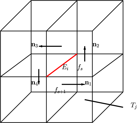
For a given interior edge $E_{i}\in{\cal E}_{h}$, assume there are $r$ elements having $E_{i}$ as one of their edges which form a solid denoted by ${\cal S}_{E_{i}}$ shown in Figure 2. Then there are $r$ interior faces $f_{j}$ ($j=1,\cdots,r$) in ${\cal S}_{E_{i}}$. Let ${\bf n}_{j}$ be a unit normal vector on the face $f_{j}$ such that normal vectors ${\bf n}_{j}$ $j=1,\cdots,r$ form oriented loop around the interior edge $E_{i}$ shown in Figure 2. For each $f_{j}$, let $\Psi_{j,1}$, $\Psi_{j,2}$ and $\Psi_{j,3}$ be the three basis functions of $V_{h}$ which are only nonzero on $f_{j}$. Define $\Theta_{j}=C_{1}\Psi_{j,1}+C_{2}\Psi_{j,2}+C_{3}\Psi_{j,3}\in V_{h}$ such that $\Theta_{j}|_{f_{j}}={\bf n}_{j}$. Define $\Lambda_{i}=\sum_{j=1}^{r}\frac{1}{|f_{j}|}\Theta_{j}$.

Unfortunately, $\Lambda_{1},\cdots,\Lambda_{N_{E}}$ are linearly dependent. Let $P_{i}$ be an interior vertex in ${\mathcal{T}}_{h}$ and ${\cal G}_{P_{i}}$ be a hull formed by the elements $T\in{\mathcal{T}}_{h}$ sharing $P_{i}$. Let $e_{j}\in{\mathcal{E}}_{h}^{0},\;j=1,\cdots,t$ with $P_{i}$ as one of its end point and $\Lambda_{j},\;j=1,\cdots,t$ be the discrete divergence free functions associated with $e_{j}$. With appropriate choosing ${\bf n}_{j}$ in defining $\Lambda_{j}$, one can prove that $\sum_{j=1}^{t}\Lambda_{j}=0$. However, if we eliminate one function from $\{\Lambda_{1},\cdots,\Lambda_{t}\}$ randomly, say $\Lambda_{1}$, we will prove that $\{\Lambda_{2},\cdots,\Lambda_{t}\}$ are linearly independent in the following lemma.

We start with $\{\Lambda_{1},\cdots,\Lambda_{N_{E}}\}$ and eliminate one function for each ${\cal G}_{P_{i}}$ for $i=1,\cdots,N_{V}$. With renumbering the functions, we end up with $N_{E}-N_{V}$ discrete divergence free functions: $\{\Lambda_{1},\cdots,\Lambda_{N_{E}-N_{V}}\}$.

In this section, we shall report several results of numerical examples for two dimensional Stokes equations. The divergence-free finite element scheme introduced in Algorithm 2 is used. The main purpose if to numerically validate the accuracy and efficiency of the WG scheme.

Let ${\bf v}_{h}\in D_{h}$ and $q_{h}\in W_{h}$, the error for the WG-FEM solution is measured in three norms defined as follows:

References

• [1] B. Cockburn, G. Kanschat, D. Schötzau, and C. Schwab, Local discontinuous Galerkin methods for the Stokes system, SIAM J. Numer. Anal., 40 (2002) 319–343.
• [2] M. Crouzeix and P. A. Raviart, Conforming and nonconforming finite element methods for solving the stationary Stokes equations, RAIRO Anal. Numer., 7 (1973) 33–76.
• [3] V. Girault and P.A. Raviart, Finite Element Methods for the Navier-Stokes Equations: Theory and Algorithms, Springer-Verlag, Berlin, 1986.
• [4] V. Girault, B. Rivière, and M.F. Wheeler, A discontinuous Gelerkin method with nonconforming domain decomposition for Stokes and Navier-Stokes problems, Math. Comp., 74 (2004) 53–84.
• [5] D. Griffiths, Finite element for incompressible flow, Math. Meth. in Appl. Sci., 1 (1979) 16–31.
• [6] D. Griffiths, The construction of approximately divergence-free finite element, The Mathematics of Finite Element an Its Applications III, Ed. J.R. Whiteman, Academic Press, 1979.
• [7] D. Griffiths, An approximately divergence-free 9-node velocity element for incompressible flows, Inter. J. Num. Meth. in Fluid, 1 (1981) 323–346.
• [8] M. D. Gunzburger, Finite Element Methods for Viscous Incompressible Flows, A Guide to Theory, Practice and Algorithms, Academic, San Diego, 1989.
• [9] K. Gustafson and R. Hartman, Divergence-free basis for finite element schemes in hydrodynamics, SIAM J. Numer. Anal., 20 (1983) 697–721.
• [10] K. Gustafson and R. Hartman, Graph theory and fluid dynamics, SIAM J. Alg. Disc. Meth., 6 (1985) 643-656.
• [11] O. A. Karakashian and W. N. Jureidini, A nonconforming finite element method for the stationary Navier-Stokes equations, SIAM J. Numerical Analysis, 35 (1998) 93–120.
• [12] J. Liu and C. Shu, A high order discontinuous Galerkin method for 2D incompressible flows, J. Comput. Phys., 160 (2000) 577–596.
• [13] J. Wang and X. Ye, A weak Galerkin finite element method for second-order elliptic problems, J. Comp. and Appl. Math, 241 (2013) 103-115.
• [14] J. Wang and X. Ye, A Weak Galerkin mixed finite element method for second-order elliptic problems, Math. Comp., 83 (2014), 2101-2126.
• [15] J. Wang and X. Ye A Weak Galerkin Finite Element Method for the Stokes Equations, Advances in Computational Mathematics, DOI 10.1007/s10444-015-9415-2, arXiv:1302.2707.
• [16] J. Wang and X. Ye, New finite element methods in computational fluid dynamics by H⁡(div)H(\rm{div}) elements, SIAM J. Numer. Anal., 45 (2007) 1269–1286.
• [17] J. Wang, X. Wang and X. Ye Finite Element Methods for the Navier-Stokes equations by H⁡(div)H(\rm{div}) Elements, Journal of Computational Mathematics, 26 (2008) 1–28.
• [18] X. Ye and C. Hall, A Discrete divergence free basis for finite element methods, Numerical Algorithms, 16 (1997) 365–380.
• [19] X. Ye and C. Hall, The Construction of null basis for a discrete divergence operator, J. Computational and Applied Mathematics, 58 (1995) 117–133.