Tackling tangledness of cosmic strings by knot polynomial topological invariants

Xinfei LI Affiliation: Institute of Theoretical Physics, Beijing University of Technology, Beijing 100124, China Xin LIU ^†^†thanks: Corresponding author: xin.liu@bjut.edu.cn Affiliation: Institute of Theoretical Physics, Beijing University of Technology, Beijing 100124, China Affiliation: Beijing-Dublin International College, Beijing University of Technology, Beijing 100124, China Yong-Chang HUANG Affiliation: Institute of Theoretical Physics, Beijing University of Technology, Beijing 100124, China

August 24, 2026

Abstract

Cosmic strings in the early universe have received revived interest in recent years. In this paper we derive these structures as topological defects from singular distributions of the quintessence field of dark energy. Our emphasis is placed on the topological charge of tangled cosmic strings, which originates from the Hopf mapping and is a Chern-Simons action possessing strong inherent tie to knot topology. It is shown that the Kauffman bracket knot polynomial can be constructed in terms of this charge for un-oriented knotted strings, serving as a topological invariant much stronger than the traditional Gauss linking numbers in characterizing string topology. Especially, we introduce a mathematical approach of breaking-reconnection which provides a promising candidate for studying physical reconnection processes within the complexity-reducing cascades of tangled cosmic strings.

§ 1. Introduction

Cosmic strings were first proposed by Kibble in 1976 from the field theoretical point of view [1]. As one-dimensional topological defects with zero width, their formation took place through a symmetry breaking phase transition (the Kibble mechanism) of an abelian Higgs model in the early universe, at the quenching stage after the cosmological inflation [2].

String theory redefines the significance of cosmic strings. A first prediction was based on F-strings, stating that a string could be produced in the early universe and stretched to macroscopic scale. But that mechanism has two potential unpleasant prospects [3]. One is, as asserted by type-I and heterotic superstring theories, that these F-strings would be produced as disintegrated small strings and appear as boundaries of domain walls, which would therefore inevitably collapse before growing into cosmic scale, due to their high tension. The other is that, in the Planck energy scale, the strings would be created prior to the cosmological inflation, and therefore get diluted away and unobservable in consequence during the inflation.

Developments of string theory overcame the above difficulties and strengthened the linkage between cosmic string and superstring theories. New one-dimensional strings were discovered, including the D-strings which correspond to F-strings via the S-duality, as well as the NS- and M-branes which have only one non-compact dimension (— the other dimensions being wrapped into an internal compact Calabi-Yau manifold with throats [4]). Low-tension strings which are stable in expanding universe are achievable now, since large compact dimensions and warp factors would suppress string tension to an observable energy scale. In 2002 Tye predicted an scenario of brane inflation where low dimensional D-branes with one non-compact dimension is produced [5]. Later, Polchinski suggested that a string could be stretched to intergalactic scale in expanding universe [6, 7]. As Kibble remarks, “string theory cosmologists have discovered cosmic strings lurking everywhere in the undergrowth”.

Therefore cosmic strings open a door to string theory; if cosmic strings could be observed it would provide the first evidence for string theory, as it is very important. At present great efforts have been put in searching observational evidence for cosmic strings, including the detections of gravitational wave radiations of string cusps and loops by the LIGO and LISA projects, Comic Microwave Background(CMB) B modes by the Planck Surveyor Mission and BICEP2, etc [8, 9, 10, 11, 12, 13].

In this paper we propose a generating mechanism for cosmic string structures, in terms of quintessence field of the dark energy. Dark energy has been thought to be a candidate to account for accelerating expansion and flatness of the universe; current measurements indicate that dark energy contributes 68.3% of the total energy of the present observable universe [11]. There are various models for dark energy such as quintessence, phantom and quintom [14, 15, 16]. In this paper we consider a $U(1)$ complex scalar model of quintessence acting as a background field of the universe,

\psi(x)=\phi^{1}(x)+i\phi^{2}(x),\hskip 28.45274pt\phi^{1},\phi^{2}\in\mathbf{R},

(1)

where $x=\left(\mathbf{x},x^{0}\right)$ denotes the coordinates of the Riemann-Cartan manifold $\mathbf{U}^{4}$ of the early universe.

In the following Sect.2 it will be shown that the singular distributions of this complex scalar field $\psi(x)$ are able to give rise to cosmic string structures. In Sect.3, after demonstrating the weakness of the traditional method of (self-)linking numbers, we will make use of the Chern-Simons type topological charge to construct the Kauffman bracket knot polynomial which is topologically a much more powerful invariant than the linking numbers. Then in Sect.4, examples of Hopf links, trefoil knots, figure-8 knots, Whitehead links and Borromean rings will be presented for reader convenience. Finally Sect.5 of Conclusion and Discussions will complete this paper.

§ 2. Cosmic strings constructed from scalar field

The quintessence model of dark energy is given by the following minimal coupling between gravity and the background field [14]

S=\int d^{4}x\sqrt{-g}\left[-\frac{1}{2}g^{\mu\nu}\partial_{\mu}\psi\partial_{\nu}\psi-V(\psi)\right],\hskip 28.45274pt\mu,\nu=1,2,3,0,

(2)

where $V(\psi)$ is a dark energy potential and model-dependent. The equation of motion reads

\partial_{\mu}\partial^{\mu}\psi-V^{\prime}(\psi)=0.

(3)

With a given a boundary condition that delivers the topological information of the base manifold, one is about to find a solution $\psi(x)$ to eq.(3). For this field $\psi$ distributed on the manifold, we are able to define a geodesic in the sense of a parallel field condition:

D_{\mu}\psi=\partial_{\mu}\psi-i\alpha A_{\mu}\psi=0,

(4)

where $\alpha=\sqrt{\hbar G/c^{3}}$ is a coupling constant and $D_{\mu}$ a covariant derivative. $A_{\mu}$ is a $U(1)$ gauge potential (i.e., a connection of principal bundle) induced by $\psi$ through eq.(4), as long as $\psi$ is regarded as a section of an associate bundle on the manifold. $A_{\mu}$ is solved out from (4) as

A_{\mu}=\frac{\alpha}{2\pi}\frac{1}{2i\psi^{*}\psi}\left(\psi^{*}\partial_{\mu}\psi-\partial_{\mu}\psi^{*}\psi\right).

(5)

Eq.(5) takes the same form of the velocity field in quantum mechanics, thanks to the London assumption of superconductivity [17]. The gauge field strength defined from $A_{\mu}$ is

F_{\mu\nu}=\partial_{\mu}A_{\nu}-\partial_{\nu}A_{\mu}.

(6)

In order to derive topological defects we introduce a two-dimensional unit vector $n^{a}$ from $\phi^{1,2}$ :

n^{a}=\frac{\phi^{a}}{\left\|\phi\right\|},\hskip 42.67912pta=1,2;~\left\|\phi\right\|^{2}=\phi^{a}\phi^{a}=\psi^{*}\psi.

(7)

Thus

A_{\mu}=\frac{\alpha}{2\pi}\epsilon_{ab}n^{a}\partial_{\mu}n^{b},\hskip 56.9055ptF_{\mu\nu}=\frac{\alpha}{2\pi}2\epsilon_{ab}\partial_{\mu}n^{a}\partial_{\nu}n^{b}.

(8)

Introducing a topological tensor current [18],

j^{\mu\nu}=\frac{1}{2}\frac{1}{\sqrt{-g}}\epsilon^{\mu\nu\lambda\rho}F_{\lambda\rho},

(9)

$F_{\mu\nu}$ can be re-expressed as a $\delta$ -function form,

j^{\mu\nu}=\frac{\alpha}{\sqrt{-g}}\delta^{2}(\mathbf{\phi})D^{\mu\nu}\left(\frac{\phi}{x}\right),

(10)

where Jacobian $\epsilon^{ab}D^{\mu\nu}\left(\frac{\phi}{x}\right)=\epsilon^{\mu\nu\lambda\rho}\partial_{\lambda}\phi^{a}\partial_{\rho}\phi^{b}$ . In deducing (10) the following relations also apply:

\partial_{\mu}n^{a}=\frac{\partial_{\mu}\phi^{a}}{\left\|\phi\right\|}+\phi^{a}\partial_{\mu}\frac{1}{\left\|\phi\right\|},\hskip 42.67912pt\partial_{a}\partial_{a}\ln\left\|\phi\right\|=2\pi\delta^{2}(\mathbf{\phi}).

In the light of the topological tensor current $j^{\mu\nu}$ a Nambu-Goto action is constructed as [19]

S=\int_{\mathbf{U}^{4}}L\sqrt{-g}d^{4}x,\hskip 28.45274pt\text{with}\hskip 28.45274ptL=\frac{1}{\alpha}\sqrt{\frac{1}{2}g_{\mu\lambda}g_{\nu\rho}j^{\mu\nu}j^{\lambda\rho}}.

(11)

Substituting (10) into (11) we arrive at an important result,

L=\frac{1}{\sqrt{-g}}\delta^{2}(\mathbf{\phi}).

(12)

Given that

\delta^{2}(\mathbf{\phi})\left\{\begin{array}[]{lll}=0,&&\text{iff }\phi^{a}\neq 0;\\ \neq 0,&&\text{iff }\phi^{a}=0,\end{array}\right.\hskip 42.67912pta=1,2,

(13)

the zero points of the $\phi^{a}$ field,

\phi^{1}(x^{1},x^{2},x^{3},x^{0})=0,\hskip 42.67912pt\phi^{2}(x^{1},x^{2},x^{3},x^{0})=0,

(14)

outline the nonzero evaluations of $L$ and indicate the presence of topological defects. According to the implicit function theorem, under the regular condition $D^{\mu\nu}\left(\frac{\phi}{x}\right)\neq 0$ , the two coupled equations of eq.(14) have the following general solutions:

P_{k}:\hskip 8.53581ptx^{\mu}=x^{\mu}_{k}(u^{I}),\hskip 42.67912ptk=1,2,\cdots,N;~I=1,2.

(15)

which are $N$ isolated 2-dimensional singular submanifolds in the four dimensional spacetime, with $u^{1},u^{2}$ being the intrinsic parameters. Thus, we achieve a model for cosmic strings by regarding $P_{k}$ ’s as the world-sheets swept by $N$ line defects, $k=1,2,\cdots,N$ , with $u^{1}=s$ as the spatial parameter and $u^{2}=t$ the temporal one, respectively.

The Lagrangian $L$ then reads

L=\frac{1}{\sqrt{-g}}\sum_{k=1}^{N}W_{k}\int_{P_{k}}\delta^{4}\left(x^{\mu}-x^{\mu}_{k}(s,t)\right)\sqrt{g_{k}}d^{2}u,

(16)

where $g_{k}=\det\left[g_{IJ}\right]$ , with $g_{IJ}$ as the intrinsic metric of the submanifold $P_{k}\left(u^{I}\right)$ . $W_{k}$ is the topological charge of $P_{k}$ , carrying the meaning of winding numbers, $W_{k}=\beta_{k}\eta_{k}$ , with $\beta_{k}$ being the Hopf index and $\eta_{k}=\pm 1$ the Brouwer degree. Thus, the action can be expressed as a sum over the actions of the individual world-sheets,

S=\sum_{k=1}^{N}W_{k}S_{k}\hskip 28.45274pt\text{with}\hskip 28.45274ptS_{k}=\int_{P_{k}}\sqrt{g_{k}}d^{2}u,

(17)

$S_{k}$ carrying the meaning of the area of $P_{k}$ .

The spatial component of the current $j^{\mu\nu}$ is given by

j^{i}=j^{0i}=\frac{\alpha}{\sqrt{-g}}\sum_{k=1}^{N}W_{k}\int_{l_{k}}\frac{dx^{i}}{ds}\delta^{3}\left(\mathbf{x}-\mathbf{x}_{k}(s)\right)ds,\hskip 28.45274pti=1,2,3.

(18)

$\frac{dx^{i}}{ds}$ gives the velocity of the $k$ th cosmic string,

\frac{dx^{i}}{ds}=\frac{D^{i}\left(\frac{\mathbf{\phi}}{x}\right)}{D\left(\frac{\mathbf{\phi}}{u}\right)}.

(19)

The motion of a string is governed by the evolution equation:

\frac{1}{\sqrt{g_{k}}}\frac{\partial}{\partial u^{I}}\left(\sqrt{g_{k}}g^{IJ}\frac{\partial x^{\mu}}{\partial u^{J}}\right)+g^{IJ}\Gamma^{\mu}_{\nu\lambda}\frac{\partial x^{\nu}}{\partial u^{I}}\frac{\partial x^{\lambda}}{\partial u^{J}}=0,\hskip 28.45274pt\mu,\nu=1,2,3,0;~I,J=1,2.

(20)

§ 3. Topological invariants for knotted cosmic strings

An ensemble of topological defects form a complex system, whose complexity is measured by its tangledness. Usually topological complexity of the system is strongly relevant to its energy and other dynamical properties: higher complexity corresponding to higher free energy or entropy, and energy release taking place during intercommutation collisions and complexity-reducing cascades [20]. Classification and characterization of topological complexity are at the center of the study of cosmic strings.

Hereinafter, we will investigate topology of cosmic strings from the mathematical point of view by studying closed strings; open strings ending at infinity will be treated as closed loops via compacticification. Thus, a string is an embedding map from a circle to the $3$ -dimensional space, $\gamma:S^{1}\rightarrow\mathbf{R}^{3}$ .

3.1 (Self-)linking numbers for knots

A knotted string with finite length has finite energy from the viewpoint of soliton study. In 1997 Faddeev and Niemi proposed a soliton model beyond the classical action of low energy Yang-Mills gauge theory, its solution providing the first $3$ -dimensional topologically stable knotted soliton solution with finite energy [21]. This model has found wide applications in physics, including trefoil knots in real fluids, protein folding in molecular biology, topological insulators exhibiting knotted 3D electronic band structure in condensed matter, etc. [22, 23, 24].

In the Faddeev-Niemi model the tangledness of knotted solitons is characterized by the topological charge

Q=\left(\frac{2\pi}{\alpha}\right)^{2}\frac{1}{4\pi}\int_{\Omega}\epsilon^{ijk}A_{i}F_{jk}d^{3}x=\frac{2\pi}{\alpha^{2}}\int_{\Omega}A_{i}j^{i}\sqrt{-g}d^{3}x,\hskip 42.67912pt\epsilon^{ijk}=\epsilon^{0ijk},

(21)

where $\Omega$ is the special volume. $A_{i}$ and $F_{ij}$ are the spatial components of $A_{\mu}$ and $F_{\mu\nu}$ , respectively. Mathematically, $Q$ is a Hopf map, $\pi_{3}(S^{2})=\mathbf{Z}$ . In the context of fluid mechanics it corresponds to an important topological invariant, helicity: $H=\int_{\Omega}\mathbf{u}\cdot\mathbf{\omega}d^{3}x$ . Here $\mathbf{u}$ is the velocity of the fluid and $\mathbf{\omega}$ the vorticity, $\mathbf{\omega}=\nabla\times\mathbf{u}$ [25]. Bekenstein pointed out that this helicity can be transplanted into the study of cosmic strings [26].

Moffatt and Ricca successfully derived an algebraic expression for $H$ as a sum of all (self-)linking numbers of knotted fluid knots [27]; the strict verification of this formula in the context of cosmic strings was given by Duan and Liu [28, 29]:

Q=2\pi\left[\sum_{k=1}^{N}W^{2}_{k}SL(\gamma_{k})+2\sum_{k,l=1(k<l)}^{N}W_{k}W_{l}Lk(\gamma_{k},\gamma_{l})\right],

(22)

where $SL(\gamma_{k})$ is the self-linking number of the $k$ th knotted string, and $LK(\gamma_{k},\gamma_{l})$ the Gauss (mutual) linking number between the $k$ th and $l$ th strings. The (self-)linking numbers are easy to obtained by counting the degree of each crossing site. By eq.(22), the initial triple integral, eq.(), is advantageously turned into simple algebraic counting.

However, from the knot theoretical point of view, (self-)linking numbers are weak knot invariants which fail to distinguish typical topology of knots/links, as shown in Figs. 1 and 2:

Refer to caption — Figure 1: Different topological configurations which have the same self-linking number $0$ : (a) a topologically trivial circle; (b) a topologically non-trivial figure-8 knot.

Therefore, in order to distinguish and characterize topology of cosmic strings we need to develop new and stronger tools of topological invariants. In the following text our starting point will still be the topological charge $Q$ of eq.21, due to a remarkable fact that $Q$ is an abelian Chern-Simons action. Chern-Simons theory is well known to be the most important topological quantum field theory in three dimensions, which provides a field theoretical framework for knot theory [30]. It is strongly relevant to knot topological invariants such as the Jones, HOMFLYPT and other knot polynomials, the Vassiliev finite type invariants via the Kontsevich integral, Khovanov homology, and so on [31, 32, 33].

In the next two subsections we will start from the Chern-Simons type topological charge $Q$ to derive the Kauffman bracket polynomial by constructing the latter’s skein relations.

3.2 Exponential form of topological charge $Q$

Substituting the $\delta$ -function expression of the current $j^{i}$ , eq.(18), into eq.(21) we obtain

Q=\frac{2\pi}{\alpha}\sum_{k=1}^{N}W_{k}\oint_{\gamma_{k}}A_{i}dx^{i}.

For convenience, in this paper we set $W_{k}=1$ and rescale $\alpha=1$ (for the cases $W_{k},\alpha\neq 1$ one can formally keep $W_{k}$ and $\alpha$ intact). Thus,

Q=2\pi\sum_{k=1}^{N}\oint_{\gamma_{k}}A_{i}dx^{i}=2\pi\oint_{L}A_{i}dx^{i},\hskip 42.67912ptL=\bigoplus\limits_{k=1}^{N}\gamma_{k},

(23)

where $L$ is the link composed of all $\gamma_{k}$ ’s. Eq.(23) means that when thin cosmic strings are considered, $Q$ can be expressed as a circular integral in the configuration space.

In this paper our main proposal is to study the exponential form of $Q$ :

e^{\frac{1}{2\pi}Q(L)}=e^{\oint_{L}A_{i}dx^{i}}.

(24)

We argue that this form is able to provide knot polynomial topological invariants such as the Kauffman bracket polynomial (see below). The advantages of this form are the following:

•

Additivity of the line integral: The link $L$ is divided into the sum of a few strands $S_{1},S_{2},S_{3},\cdots$ in the configuration space, $L=S_{1}\oplus S_{2}\oplus S_{3}\oplus\cdots$ , as shown in Fig.3.

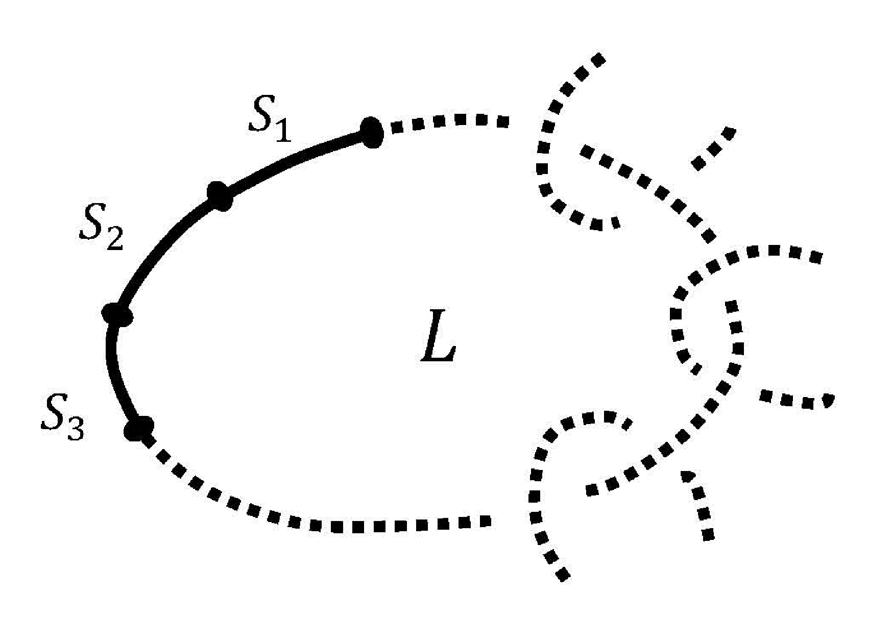
Figure 3: The link $L$ is additive, i.e., it can be treated as the sum of all the strands $S_{1},S_{2},S_{3},\cdots$ .

Then the line integral over the path $L$ has the feature of additivity:

$\oint_{L}=\int_{S_{1}}+\int_{S_{2}}+\int_{S_{3}}+\cdots.$ (25)
•

Factorization of the exponential form: The addition in the power of the exponential leads to

$e^{\oint_{L}}=e^{\int_{S_{1}}}e^{\int_{S_{2}}}e^{\int_{S_{3}}}\cdots.$ (26)

This provides us a pathway to construct the formal parameter $a$ in the skein relations of the Kauffman bracket polynomial.

We introduce a bracket symbol to denote the exponential of the line integral over a link $L$ :

\left\langle L\right\rangle=e^{\oint_{L}A_{i}dx^{i}}.

(27)

An immediate application is the case that $L$ is a trivial circle :

\left\langle\begin{picture}(0.2,0.5)\put(1.0,1.0){\circle{1.2}}\end{picture}\right\rangle=e^{\oint_{\begin{picture}(0.2,0.5)\put(1.0,1.0){\circle{1.2}}\end{picture}}A_{i}dx^{i}}=e^{\frac{1}{2}\iint_{\Sigma}F_{ij}dx^{i}\wedge dx^{j}}=e^{0}=1,

(28)

where the Stokes’ theorem applies.

3.3 Kauffman bracket knot polynomial topological invariant

To keep in accordance with the knot theoretical routine, let us start from examining the three basic states at a crossing site: the over-, under- and non-crossings, as shown in Fig4.

An example is that, if joining the two right ends in each configuration of Fig.4, we obtain the ones of Fig.5: (a) $\alpha_{+}$ , (b) $\alpha_{-}$ , and (c) $\alpha_{0}=\begin{picture}\put(0.9,-0.5){\line{0}{1}{2.0}}\end{picture}\cup\begin{picture}(0.2,0.5)\put(1.0,1.0){\circle{1.2}}\end{picture}$ and $\alpha_{\infty}=\begin{picture}\put(0.9,-0.5){\line{0}{1}{2.0}}\end{picture}$ .

Furthermore, for convenience, we introduce the following notations for two important writhing loops:

\gamma_{+}=\begin{picture}(-8.0,-2.0)\qbezier{}{1.4}{-1.8}{2}{-2.7}{3.2}{-2.9}\qbezier{}{3.2}{-2.9}{6}{-2.7}{6.2}{-0.2}\qbezier{}{6.2}{-0.2}{5.9}{2.6}{3.1}{2.9}\qbezier{}{3.1}{2.9}{0.3}{2.6}{0}{0}\qbezier{}{-1.4}{1.8}{-2}{2.7}{-3.2}{2.9}\qbezier{}{-3.2}{2.9}{-6}{2.7}{-6.2}{0.2}\qbezier{}{-6.2}{0.2}{-5.9}{-2.6}{-3.1}{-2.9}\qbezier{}{-3.1}{-2.9}{-0.3}{-2.6}{0}{0}\end{picture},\hskip 42.67912pt\gamma_{-}=\begin{picture}(-8.0,-2.0)\qbezier{}{-1.4}{-1.8}{-2}{-2.7}{-3.2}{-2.9}\qbezier{}{-3.2}{-2.9}{-6}{-2.7}{-6.2}{-0.2}\qbezier{}{-6.2}{-0.2}{-5.9}{2.6}{-3.1}{2.9}\qbezier{}{-3.1}{2.9}{-0.3}{2.6}{0}{0}\qbezier{}{1.4}{1.8}{2}{2.7}{3.2}{2.9}\qbezier{}{3.2}{2.9}{6}{2.7}{6.2}{0.2}\qbezier{}{6.2}{0.2}{5.9}{-2.6}{3.1}{-2.9}\qbezier{}{3.1}{-2.9}{0.3}{-2.6}{0}{0}\end{picture}.

The over- and under-crossings $L_{+}$ and $L_{-}$ , as integration paths in the sense of eq.(23), can be locally decomposed in different ways in the configuration space. Taking $L_{+}$ for example, it has two decomposing channels, the left-right (LR) and the up-down (UD), as showed in Fig. 6 (for details see [34, 35]):

Adopting ergodic statistical hypothesis, we argue that these two channels should have equal contributions to $e^{\frac{1}{2\pi}Q\left(L_{+}\right)}$ when modifying the integration paths of $L_{+}$ :

	$\displaystyle e^{\frac{1}{2\pi}Q(L_{+})}=\left\langle L_{+}\right\rangle=\left\langle L_{+}\text{-- LR}\right\rangle+\left\langle L_{+}\text{-- UD}\right\rangle,$	(29)
where	$\displaystyle\left\langle L_{+}\text{-- LR}\right\rangle=e^{\oint_{L_{0}\oplus\gamma_{+}}}=e^{\oint_{L_{0}}}e^{\oint_{\gamma_{+}}},$	(30)
	$\displaystyle\left\langle L_{+}\text{-- UD}\right\rangle=e^{\oint_{L_{\infty}\oplus\gamma_{-}}}=e^{\oint_{L_{\infty}}}e^{\oint_{\gamma_{-}}}.$	(31)

Denoting $e^{\oint_{\gamma_{+,-}}}$ as

	$\displaystyle e^{\oint_{\gamma_{+}}}$	$\displaystyle=$	$\displaystyle\exp\left(\oint_{\begin{picture}(-8.0,-2.0)\qbezier{}{1.4}{-1.8}{2}{-2.7}{3.2}{-2.9}\qbezier{}{3.2}{-2.9}{6}{-2.7}{6.2}{-0.2}\qbezier{}{6.2}{-0.2}{5.9}{2.6}{3.1}{2.9}\qbezier{}{3.1}{2.9}{0.3}{2.6}{0}{0}\qbezier{}{-1.4}{1.8}{-2}{2.7}{-3.2}{2.9}\qbezier{}{-3.2}{2.9}{-6}{2.7}{-6.2}{0.2}\qbezier{}{-6.2}{0.2}{-5.9}{-2.6}{-3.1}{-2.9}\qbezier{}{-3.1}{-2.9}{-0.3}{-2.6}{0}{0}\end{picture}}A_{i}dx^{i}\right)=a,$		(32)
	$\displaystyle e^{\oint_{\gamma_{-}}}$	$\displaystyle=$	$\displaystyle\exp\left(\oint_{\begin{picture}(-8.0,-2.0)\qbezier{}{-1.4}{-1.8}{-2}{-2.7}{-3.2}{-2.9}\qbezier{}{-3.2}{-2.9}{-6}{-2.7}{-6.2}{-0.2}\qbezier{}{-6.2}{-0.2}{-5.9}{2.6}{-3.1}{2.9}\qbezier{}{-3.1}{2.9}{-0.3}{2.6}{0}{0}\qbezier{}{1.4}{1.8}{2}{2.7}{3.2}{2.9}\qbezier{}{3.2}{2.9}{6}{2.7}{6.2}{0.2}\qbezier{}{6.2}{0.2}{5.9}{-2.6}{3.1}{-2.9}\qbezier{}{3.1}{-2.9}{0.3}{-2.6}{0}{0}\end{picture}}A_{i}dx^{i}\right)=\exp\left(-\oint_{\begin{picture}(-8.0,-2.0)\qbezier{}{1.4}{-1.8}{2}{-2.7}{3.2}{-2.9}\qbezier{}{3.2}{-2.9}{6}{-2.7}{6.2}{-0.2}\qbezier{}{6.2}{-0.2}{5.9}{2.6}{3.1}{2.9}\qbezier{}{3.1}{2.9}{0.3}{2.6}{0}{0}\qbezier{}{-1.4}{1.8}{-2}{2.7}{-3.2}{2.9}\qbezier{}{-3.2}{2.9}{-6}{2.7}{-6.2}{0.2}\qbezier{}{-6.2}{0.2}{-5.9}{-2.6}{-3.1}{-2.9}\qbezier{}{-3.1}{-2.9}{-0.3}{-2.6}{0}{0}\end{picture}}A_{i}dx^{i}\right)=a^{-1},$		(33)

eq.(29) becomes

\left\langle\begin{picture}(-1.3,-0.6)\qbezier{}{-1}{-1}{0}{0}{1}{1}\qbezier{}{-0.3}{0.3}{-0.8}{0.8}{-1}{1}\qbezier{}{0.3}{-0.3}{0.8}{-0.8}{1}{-1}\end{picture}\right\rangle=a\left\langle\begin{picture}(-1.0,2.0)\qbezier{}{0}{0}{4}{4}{0}{8}\qbezier{}{6}{0}{2}{4}{6}{8}\end{picture}\right\rangle+a^{-1}\left\langle\begin{picture}(-1.0,1.0)\qbezier{}{0}{6}{4}{2}{8}{6}\qbezier{}{0}{0}{4}{4}{8}{0}\end{picture}\right\rangle,

(34)

where

\left\langle\begin{picture}(-1.3,-0.6)\qbezier{}{-1}{-1}{0}{0}{1}{1}\qbezier{}{-0.3}{0.3}{-0.8}{0.8}{-1}{1}\qbezier{}{0.3}{-0.3}{0.8}{-0.8}{1}{-1}\end{picture}\right\rangle=e^{\oint_{L_{+}}},\hskip 42.67912pt\left\langle\begin{picture}(-1.0,2.0)\qbezier{}{0}{0}{4}{4}{0}{8}\qbezier{}{6}{0}{2}{4}{6}{8}\end{picture}\right\rangle=e^{\oint_{L_{0}}},\hskip 42.67912pt\left\langle\begin{picture}(-1.0,1.0)\qbezier{}{0}{6}{4}{2}{8}{6}\qbezier{}{0}{0}{4}{4}{8}{0}\end{picture}\right\rangle=e^{\oint_{L_{\infty}}}.

(35)

Similarly, $e^{\frac{1}{2\pi}Q(L_{-})}$ has the decomposition

\left\langle\begin{picture}(-1.3,-0.6)\qbezier{}{1}{-1}{0}{0}{-1}{1}\qbezier{}{0.3}{0.3}{0.8}{0.8}{1}{1}\qbezier{}{-0.3}{-0.3}{-0.8}{-0.8}{-1}{-1}\end{picture}\right\rangle=a^{-1}\left\langle\begin{picture}(-1.0,2.0)\qbezier{}{0}{0}{4}{4}{0}{8}\qbezier{}{6}{0}{2}{4}{6}{8}\end{picture}\right\rangle+a\left\langle\begin{picture}(-1.0,1.0)\qbezier{}{0}{6}{4}{2}{8}{6}\qbezier{}{0}{0}{4}{4}{8}{0}\end{picture}\right\rangle,\hskip 28.45274pt\text{with~~~}\left\langle\begin{picture}(-1.3,-0.6)\qbezier{}{1}{-1}{0}{0}{-1}{1}\qbezier{}{0.3}{0.3}{0.8}{0.8}{1}{1}\qbezier{}{-0.3}{-0.3}{-0.8}{-0.8}{-1}{-1}\end{picture}\right\rangle=e^{\oint_{L_{-}}}.

(36)

The evaluation of $a$ gives the directional writhing number of : $a=e^{\lambda}$ , where $\lambda$ ranges within $[0,1]$ , reflecting the direction to observe the writhe. The statistical average of $\lambda$ reads $\bar{\lambda}=\frac{1}{2}$ , thus $\bar{a}=e^{\frac{1}{2}}$ .

Eqs.(34) and (36) account for the two skein relations describing crossings. To obtain another skein relation describing the disjoint union $\left\langle\begin{picture}\put(0.9,-0.5){\line{0}{1}{2.0}}\end{picture}\cup\begin{picture}(0.2,0.5)\put(1.0,1.0){\circle{1.2}}\end{picture}\right\rangle$ , we notice the following splitting decompositions:

e^{\oint_{\alpha_{+}}}=\exp\left(\oint_{\begin{picture}\put(0.9,-0.5){\line{0}{1}{2.0}}\end{picture}\cup\begin{picture}(0.2,0.5)\put(1.0,1.0){\circle{1.2}}\end{picture}}\right)\exp\left(\oint_{\gamma_{+}}\right),\hskip 28.45274pte^{\oint_{\alpha_{-}}}=\exp\left(\oint_{\begin{picture}\put(0.9,-0.5){\line{0}{1}{2.0}}\end{picture}\cup\begin{picture}(0.2,0.5)\put(1.0,1.0){\circle{1.2}}\end{picture}}\right)\exp\left(\oint_{\gamma_{-}}\right),

(37)

illustrated by

This means we have two channels to derive $\left\langle\begin{picture}\put(0.9,-0.5){\line{0}{1}{2.0}}\end{picture}\cup\begin{picture}(0.2,0.5)\put(1.0,1.0){\circle{1.2}}\end{picture}\right\rangle$ as shown in Fig.8:

As per the ergodic statistical hypothesis these two channels should have the equal contribution to $\left\langle\begin{picture}\put(0.9,-0.5){\line{0}{1}{2.0}}\end{picture}\cup\begin{picture}(0.2,0.5)\put(1.0,1.0){\circle{1.2}}\end{picture}\right\rangle$ ; hence,

\left\langle\begin{picture}\put(0.9,-0.5){\line{0}{1}{2.0}}\end{picture}\cup\begin{picture}(0.2,0.5)\put(1.0,1.0){\circle{1.2}}\end{picture}\right\rangle=a^{-1}\left\langle\begin{picture}(-2.0,-6.0)\qbezier{}{1.4}{-5.2}{2}{-6.2}{3.2}{-6.1}\qbezier{}{3.2}{-6.2}{6}{-6.2}{6.2}{-3.1}\qbezier{}{6.2}{-3.1}{5.9}{-0.3}{3.1}{-0}\qbezier{}{3.1}{-0}{0.3}{-0.3}{0}{-2.9}\put(0.0,-3.1){\line{0}{-1}{7.0}}\put(0.0,0.8){\line{0}{1}{4.0}}\end{picture}\right\rangle+\left(a^{-1}\right)^{-1}\left\langle\begin{picture}(-2.0,0.0)\qbezier{}{1.4}{5.2}{2}{6.2}{3.2}{6.1}\qbezier{}{3.2}{6.2}{6}{6.2}{6.2}{3.1}\qbezier{}{6.2}{3.1}{5.9}{0.3}{3.1}{0}\qbezier{}{3.1}{0}{0.3}{0.3}{0}{2.9}\put(0.0,3.1){\line{0}{1}{7.0}}\put(0.0,-0.8){\line{0}{-1}{4.0}}\end{picture}\right\rangle=a^{-1}\left\langle\begin{picture}(-2.0,-6.0)\qbezier{}{1.4}{-5.2}{2}{-6.2}{3.2}{-6.1}\qbezier{}{3.2}{-6.2}{6}{-6.2}{6.2}{-3.1}\qbezier{}{6.2}{-3.1}{5.9}{-0.3}{3.1}{-0}\qbezier{}{3.1}{-0}{0.3}{-0.3}{0}{-2.9}\put(0.0,-3.1){\line{0}{-1}{7.0}}\put(0.0,0.8){\line{0}{1}{4.0}}\end{picture}\right\rangle+a\left\langle\begin{picture}(-2.0,0.0)\qbezier{}{1.4}{5.2}{2}{6.2}{3.2}{6.1}\qbezier{}{3.2}{6.2}{6}{6.2}{6.2}{3.1}\qbezier{}{6.2}{3.1}{5.9}{0.3}{3.1}{0}\qbezier{}{3.1}{0}{0.3}{0.3}{0}{2.9}\put(0.0,3.1){\line{0}{1}{7.0}}\put(0.0,-0.8){\line{0}{-1}{4.0}}\end{picture}\right\rangle.

(38)

On the other hand, (resp., ) can be obtained by joining the two right ends of (resp., ). Thus eqs.(34) and (36) yields

	$\displaystyle\left\langle\begin{picture}(-2.0,-6.0)\qbezier{}{1.4}{-5.2}{2}{-6.2}{3.2}{-6.1}\qbezier{}{3.2}{-6.2}{6}{-6.2}{6.2}{-3.1}\qbezier{}{6.2}{-3.1}{5.9}{-0.3}{3.1}{-0}\qbezier{}{3.1}{-0}{0.3}{-0.3}{0}{-2.9}\put(0.0,-3.1){\line{0}{-1}{7.0}}\put(0.0,0.8){\line{0}{1}{4.0}}\end{picture}\right\rangle$	$\displaystyle=$	$\displaystyle a\left\langle\begin{picture}\put(0.9,-0.5){\line{0}{1}{2.0}}\end{picture}\cup\begin{picture}(0.2,0.5)\put(1.0,1.0){\circle{1.2}}\end{picture}\right\rangle+a^{-1}\left\langle\begin{picture}\put(0.9,-0.5){\line{0}{1}{2.0}}\end{picture}\right\rangle,$		(39)
	$\displaystyle\left\langle\begin{picture}(-2.0,0.0)\qbezier{}{1.4}{5.2}{2}{6.2}{3.2}{6.1}\qbezier{}{3.2}{6.2}{6}{6.2}{6.2}{3.1}\qbezier{}{6.2}{3.1}{5.9}{0.3}{3.1}{0}\qbezier{}{3.1}{0}{0.3}{0.3}{0}{2.9}\put(0.0,3.1){\line{0}{1}{7.0}}\put(0.0,-0.8){\line{0}{-1}{4.0}}\end{picture}\right\rangle$	$\displaystyle=$	$\displaystyle a^{-1}\left\langle\begin{picture}\put(0.9,-0.5){\line{0}{1}{2.0}}\end{picture}\cup\begin{picture}(0.2,0.5)\put(1.0,1.0){\circle{1.2}}\end{picture}\right\rangle+a\left\langle\begin{picture}\put(0.9,-0.5){\line{0}{1}{2.0}}\end{picture}\right\rangle,$		(40)

Combining eqs.(38), (39) and (40), we arrive at

\left\langle\begin{picture}\put(0.9,-0.5){\line{0}{1}{2.0}}\end{picture}\cup\begin{picture}(0.2,0.5)\put(1.0,1.0){\circle{1.2}}\end{picture}\right\rangle=\left(-a^{-2}-a^{2}\right)\left\langle\begin{picture}\put(0.9,-0.5){\line{0}{1}{2.0}}\end{picture}\right\rangle.

(41)

Then, in summary, we have achieved the skein relations of the Kauffman bracket polynomial, i.e., eqs.(28), (34), (36) and (41):

	$\displaystyle\left\langle\begin{picture}(0.2,0.5)\put(1.0,1.0){\circle{1.2}}\end{picture}\right\rangle=1,$		(42)
	$\displaystyle\left\langle\begin{picture}(-1.3,-0.6)\qbezier{}{-1}{-1}{0}{0}{1}{1}\qbezier{}{-0.3}{0.3}{-0.8}{0.8}{-1}{1}\qbezier{}{0.3}{-0.3}{0.8}{-0.8}{1}{-1}\end{picture}\right\rangle=a\left\langle\begin{picture}(-1.0,2.0)\qbezier{}{0}{0}{4}{4}{0}{8}\qbezier{}{6}{0}{2}{4}{6}{8}\end{picture}\right\rangle+a^{-1}\left\langle\begin{picture}(-1.0,1.0)\qbezier{}{0}{6}{4}{2}{8}{6}\qbezier{}{0}{0}{4}{4}{8}{0}\end{picture}\right\rangle,\hskip 28.45274pt\left\langle\begin{picture}(-1.3,-0.6)\qbezier{}{1}{-1}{0}{0}{-1}{1}\qbezier{}{0.3}{0.3}{0.8}{0.8}{1}{1}\qbezier{}{-0.3}{-0.3}{-0.8}{-0.8}{-1}{-1}\end{picture}\right\rangle=a^{-1}\left\langle\begin{picture}(-1.0,2.0)\qbezier{}{0}{0}{4}{4}{0}{8}\qbezier{}{6}{0}{2}{4}{6}{8}\end{picture}\right\rangle+a\left\langle\begin{picture}(-1.0,1.0)\qbezier{}{0}{6}{4}{2}{8}{6}\qbezier{}{0}{0}{4}{4}{8}{0}\end{picture}\right\rangle,$		(43)
	$\displaystyle\left\langle\begin{picture}\put(0.9,-0.5){\line{0}{1}{2.0}}\end{picture}\cup\begin{picture}(0.2,0.5)\put(1.0,1.0){\circle{1.2}}\end{picture}\right\rangle=\left(-a^{-2}-a^{2}\right)\left\langle\begin{picture}\put(0.9,-0.5){\line{0}{1}{2.0}}\end{picture}\right\rangle.$		(44)

An additional remark is that the Jones polynomial for oriented knots/links is able to be constructed from the Kauffman bracket polynomial for un-oriented ones. See Refs.[36, 34].

§ 4. Examples

In this section the Kauffman bracket polynomials of some typical elementary configurations are presented for reader convenience.

4.1 Disjoint union of trivial circles

Let us start from considering the union of two circles. In terms of (44) we have

\left\langle\begin{picture}(0.2,0.5)\put(1.0,1.0){\circle{1.2}}\end{picture}\cup\begin{picture}(0.2,0.5)\put(1.0,1.0){\circle{1.2}}\end{picture}\right\rangle=\left(-a^{-2}-a^{2}\right)\left\langle\begin{picture}(0.2,0.5)\put(1.0,1.0){\circle{1.2}}\end{picture}\right\rangle=-a^{-2}-a^{2}.

This result can be easily generalized to the case of $n$ circles:

\left\langle\overset{n\text{ copies}}{\overbrace{\begin{picture}(0.2,0.5)\put(1.0,1.0){\circle{1.2}}\end{picture}\cup\begin{picture}(0.2,0.5)\put(1.0,1.0){\circle{1.2}}\end{picture}\cup\cdots\cup\begin{picture}(0.2,0.5)\put(1.0,1.0){\circle{1.2}}\end{picture}}}\right\rangle=\left(-a^{-2}-a^{2}\right)^{n-1}.

(45)

4.2 Hopf link, $H$

Consider a Hopf link, denoted as $H$ , as shown in the top row of Fig.9. Applying the skein relation (43) to its upper crossing site, we have

\left\langle H\right\rangle=a\left\langle H_{A}\right\rangle+a^{-1}\left\langle H_{B}\right\rangle,

(46)

where $H_{A}$ and $H_{B}$ are the two states in the middle row of Fig.9. Further, continuing to apply (43) to the lower crossing site of $H_{A}$ , we have

\left\langle H_{A}\right\rangle=a\left\langle H_{1}\right\rangle+a^{-1}\left\langle H_{2}\right\rangle,

(47)

where $H_{1}$ and $H_{2}$ are two states in the bottom row of Fig.10. Similarly, $H_{B}$ satisfies

\left\langle H_{B}\right\rangle=a\left\langle H_{3}\right\rangle+a^{-1}\left\langle H_{4}\right\rangle.

(48)

Substituting (47) and (48) into (46) we have

\left\langle H\right\rangle=aa\left\langle H_{1}\right\rangle+aa^{-1}\left\langle H_{2}\right\rangle+a^{-1}a\left\langle H_{3}\right\rangle+a^{-1}a^{-1}\left\langle H_{4}\right\rangle.

(49)

This expression can be understood as follows. It contains four items respectively corresponding to the four states in the bottom row. Each item, say $aa\left\langle H_{1}\right\rangle$ , has two factors: $\left\langle H_{1}\right\rangle$ , the polynomial of the state; $aa$ , the path from the top $H$ to the bottom $H_{1}$ via the middle $H_{A}$ .

In the light of eq.(45), one can see that $\left\langle H_{1}\right\rangle=-a^{2}-a^{-2}$ , since $H_{1}$ the disjointed union of two trivial circles. Similarly, the bracket polynomials of the other three states $H_{2}$ , $H_{3}$ and $H_{4}$ are

$H_{1}$	$-a^{2}-a^{-2}$	$H_{2}$	$1$
$H_{3}$	$1$	$H_{4}$	$-a^{2}-a^{-2}$

Then, substituting these values into (49) we achieve the Kauffman bracket polynomial of the Hopf link:

\left\langle H\right\rangle=-a^{-4}-a^{4}.

(50)

The above method can be extended to a generic case. For a link $L$ , its Kauffman bracket polynomial is given by [36]

\left\langle L\right\rangle=\sum_{s}a^{\theta_{0}(s)}a^{-\theta_{\infty}(s)}\left(-a^{-2}-a^{2}\right)^{\left|s\right|-1},

(51)

where the sum is done over all the states in the bottom row. For a state, say $s$ , supposing it is the disjoint union of $\left|s\right|$ circles, and from the top $L$ to this state $s$ the path contains $\theta_{0}(s)$ LR-splittings and $\theta_{\infty}(s)$ UD-splittings, the summand corresponding to $s$ reads: $a^{\theta_{0}(s)}a^{-\theta_{\infty}(s)}\left(-a^{-2}-a^{2}\right)^{\left|s\right|-1}$ .

4.3 Trefoil knots, $T^{R}$ and $T^{L}$

In the light of eq.(51), we have the bracket polynomials for each state in the bottom row of Fig.10:

$T_{1}$	$-a^{3}(a^{2}+a^{-2})$	$T_{2}$	$a$	$T_{3}$	$a$
$T_{4}$	$-a^{-1}(a^{2}+a^{-2})$	$T_{5}$	$a$	$T_{6}$	$-a^{-1}(a^{2}+a^{-2})$
$T_{7}$	$-a^{-1}(a^{2}+a^{-2})$	$T_{8}$	$-a^{-3}(a^{2}+a^{-2})^{2}$

Summing up all the contributions of the states $T_{1}$ — $T_{8}$ , we achieve the Kauffman bracket for the right-handed trefoil knot $T^{R}$ :

\left\langle T^{R}\right\rangle=a^{-7}-a^{-3}-a^{5}.

(52)

Similarly, the polynomial of the left-handed trefoil knot $T^{L}$ (i.e., the mirror image of $T^{R}$ ) reads

\left\langle T^{L}\right\rangle=-a^{-5}-a^{3}+a^{7}.

(53)

Obviously, the Kauffman bracket polynomial is able to distinguish the right- and left-handed trefoil knots.

4.4 Figure-8 knot, $F^{8}$

A Figure-8 knot, denoted as $F^{8}$ , can be decomposed into the two states $A$ and $B$ in Fig.11:

Thus

\left\langle F^{8}\right\rangle=a\left\langle A\right\rangle+a^{-1}\left\langle B\right\rangle.

(54)

The further decomposition of $A$ is given in Fig.12:

where the polynomials for each of the states $A_{1}$ — $A_{8}$ are

$A_{1}$	$a^{4}(a^{-2}+a^{2})^{2}$	$A_{2}$	$-a^{2}(a^{-2}+a^{2})$	$A_{3}$	$-a^{2}(a^{-2}+a^{2})$	$A_{4}$	$(a^{-2}+a^{2})^{2}$
$A_{5}$	$-a^{2}(a^{-2}+a^{2})$	$A_{6}$	1	$A_{7}$	1	$A_{8}$	$-a^{2}(a^{-2}+a^{2})$

The decomposition of $B$ is given in Fig.13:

where the polynomials for each of the states $B_{1}$ — $B_{8}$ are

$B_{1}$	$-a^{2}(a^{-2}+a^{2})$	$B_{2}$	1	$B_{3}$	1	$B_{4}$	$-a^{2}(a^{-2}+a^{2})$
$B_{5}$	$1$	$B_{6}$	$-a^{-2}(a^{-2}+a^{2})$	$B_{7}$	$-a^{-2}(a^{-2}+a^{2})$	$B_{8}$	$-a^{4}(a^{-2}+a^{2})^{2}$

Substituting states $A_{1}$ — $A_{8}$ and $B_{1}$ — $B_{8}$ into eq.(54), we achieve the Kauffman bracket polynomial for the Figure-8 knot:

\left\langle F^{8}\right\rangle=a^{-8}-a^{-4}+1-a^{4}+a^{8}.

(55)

An immediate conclusion is that the Kauffman polynomial is able to distinguish a trivial circle and a Figure-8 knot, the two topologically different configurations of Fig.1.

4.5 Borromean rings and Whitehead link

The Kauffman polynomials of the Borromean rings and the Whitehead links are computed as

	$\displaystyle\left\langle\text{Borromean rings}\right\rangle=-a^{-12}+3a^{-8}-2a^{-4}+4-2a^{4}+3a^{8}-a^{12},$		(56)
	$\displaystyle\left\langle\text{Whitehead links}\right\rangle=a^{-9}-a^{-5}+2a^{-1}-a^{3}+2a^{7}-a^{11}.$		(57)

Meanwhile from eq.(45) we have the polynomial for three trivial circles

\left\langle\text{Three circles}\right\rangle=a^{-4}+2+a^{4}.

(58)

Therefore the three topologically different configurations of Fig. 2 can be successfully distinguished by the Kauffman bracket polynomial.

§ 5. Conclusion and Discussion

In this paper cosmic strings in the early universe are achieved as one-dimensional topological defects in the $U(1)$ complex scalar quintessence field of dark energy. Our starting point is the abelian Chern-Simons type topological charge $Q$ . We propose to study its exponential form, and argue that the Kauffman bracket knot polynomial, a topological invariant much stronger than the traditional tool of (self-)linking numbers, can be constructed from this form. This opens a new door to investigation of structural complexity of extensive tangled cosmic strings in terms of classical field theory. Moreover, typical elementary examples of Hopf links, trefoil knots, figure-8 knot, Whitehead links and Borromean rings are presented for reader convenience.

Discussion: reconnection of cosmic strings

In Subsection 3.3 we introduced a mathematical approach of breaking-reconnection, i.e., the technique of addition/subtraction of imaginary local paths together with ergodic statistical hypothesis. This provides a promising candidate for studying the physical reconnection processes of tangled cosmic strings within complexity-reducing cascades.

When moving towards each other, two cosmic strings probably cross and exchange strands, somehow like the production and annihilation of kink/anti-kink pairs. This reconnection process has strong linkage to string compactification and coupling with certain relative velocities, intersection angles and string strengths (see [37, 38, 39] for discussions of dynamical aspects of kinks in small and large scales).

Major reconnection processes include intercommunication and loop formation, as shown in Fig.14. Tiny twisted circle-shaped objects are produced during the processes, causing topological conservation breaking and energy dissipation via gravitational radiation [40]. After a series of reconnection events, knotted cosmic strings tend to reach a stable stage, where only the strings with much less tangledness are left, and trivial circles and long open strings terminate at the boundary.

Figs.6 and 7 above provide us a hint for studying these topologically nonconservative events with energy dissipation. An important fact observed is that, when the crossings and degenerate to and , they are always accompanied by the emergence of the writhing structures $\gamma_{\pm}$ , and ; the same thing happens to the degeneration from the nontrivial and to the trivial . The tiny structures $\gamma_{\pm}$ might play the role of a topological-conservation breaker and lost-energy carrier, which has potential significance for future study of energy dissipation in reconnection processes of tangled cosmic strings.

§ 6. Acknowledgements

We are grateful to Professor Renzo L. Ricca for helpful discussions. X.L. was financially supported by the National Natural Science Foundation of China (NSFC, No.11572005) and the Youth Fellowship of the Haiju Project of Beijing. Y.C.H. was supported by the NSFC (No. 11275017 and 11173028).

References

$[{1}]$ T.W.B. Kibble, Topology of cosmic domains and string, J. Phys. A 9 (1976) 1387.
$[{2}]$ A. Rajantie, Defect formation in the early universe, Contemp. Phys. 44 (2003) 485.
$[{3}]$ E. Witten, Cosmic superstrings, Phys. Lett. B 153 (1985) 243.
$[{4}]$ S. Kachru, R. Kallosh, A.D. Linde, J.M. Maldacena, L.P. McAllister and S.P. Trivedi, Towards inflation in string theory, J. Cosmol. Astropart. Phys. 0310 (2003) 013.
$[{5}]$ S. Sarangi and S.H.H. Tye, Cosmic string production towards the end of brane inflation, Phys. Lett. B 536 (2002) 185.
$[{6}]$ E.J. Copeland, R.C. Myers and J. Polchinski, Cosmic F and D strings, J. High Energy Phys. 0406 (2004) 013.
$[{7}]$ J. Polchinski, Cosmic superstrings revisited, Int. J. Mod. Phys. A 20 (2005) 3413.
$[{8}]$ M.I. Cohen, C. Cutler and M. Vallisneri, Searches for cosmic-string gravitational-wave bursts in mock LISA data, Class. Quant. Grav. 27 (2010) 185012.
$[{9}]$ S. Henrot-Versille et al., Improved constraint on the primordial gravitational-wave density using recent cosmological data and its impact on cosmic string models, Class. Quant. Grav. 32 (2015) 045003.
$[{10}]$ A. Moss and L. Pogosian, Did BICEP2 see vector modes? First B-mode constraints on cosmic defects, Phys. Rev. Lett. 112 (2014) 171302.
$[{11}]$ P.A.R. Ade et al., Planck 2013 results. I. Overview of products and scientific results, Astron. Astrophys. 571 (2014) A1.
$[{12}]$ P.A.R. Ade et al., Planck 2013 results. XXV. Searches for cosmic strings and other topological defects, Astron. Astrophys. 571 (2014) A25.
$[{13}]$ J. Aasi et al., Constraints on cosmic strings from the LIGO-Virgo gravitational-wave detectors, Phys. Rev. Lett. 112 (2014) 131101.
$[{14}]$ C. Witterich, Cosmology and the fate of dilatation symmetry, Nucl.Phys. B 302 (1988) 668.
$[{15}]$ P.J. Steinhardt, L.M. Wang and I. Zlatev, Cosmological tracking solutions, Phys. Rev. D 59 (1999) 123504.
$[{16}]$ B. Feng, X.L. Wang and X.M. Zhang, Dark energy constraints from the cosmic age and supernova, Phys. Lett. B 607 (2005) 35.
$[{17}]$ Y.-S. Duan, X. Liu and P.-M. Zhang, Decomposition theory of the U(1) gauge potential and the London assumption in topological field dynamics, J. Phys.: Condens. Matter 14 (2002) 7941.
$[{18}]$ Y.-S. Duan, L.-B. Fu and G. Jia, Topological tensor current of dual $p$ -branes in the $\phi$ -mapping theory, J. Math. Phys. 41 (2000) 4379.
$[{19}]$ H.B. Nielsen and P. Olesen, Vortex-line models for dual strings, Nucl. Phys.B 61 (1973) 45.
$[{20}]$ D. Kleckner, L.H. Kauffman and W.T.M. Irvine, How superfluid vortex knots untie, Pre-eprint [arXiv:1507.07579].
$[{21}]$ L.D. Faddeev and A.J. Niemi, A stable knot-like structures in classical field theory. Nature 387 (1997) 58.
$[{22}]$ D. Kleckner, W.T.M. Irvine. Creation and dynamics of knotted vortices, Nature Physics 9 (2013) 253.
$[{23}]$ E. Shakhnovich, Protein folding: To knot or not to knot? Nature Materials 10 (2011) 84.
$[{24}]$ J.E. Moore, The birth of topological insulators, Nature 464 (2010) 194.
$[{25}]$ H.K. Moffat, The degree of knottedness of tangled vortes lines, J. Fluid Mech. 35 (1969) 117.
$[{26}]$ J.D. Bekenstein, Conservation law for linked cosmic string loops, Phys. Lett. B 282 (1992) 44.
$[{27}]$ R.L. Ricca and H.K. Moffatt, The helicity of a knotted vortex filament, H.K.Moffat, et al.(eds) Topological aspects of the dynamics of fluids and plasmas, Springer, 218 (1992) 215.
$[{28}]$ Y.-S. Duan, X. Liu and L.-B. Fu, Many knots in Chern-Simons field theory, Phys. Rev. D 67 (2003) 085022.
$[{29}]$ Y.-S. Duan and X. Liu, Knot-like cosmic strings in the early universe, J. High Energy Phys. 0402 (2004) 028.
$[{30}]$ E. Witten, Quantum field theory and the Jones polynomial, Commun. Math. Phys. 121 (1989) 351.
$[{31}]$ J.S. Birman and X.-S. Lin, Knot polynomials and Vassiliev’s invariants, Invent. Math 111 (1993) 225.
$[{32}]$ I. Kofman and X.-S., Lin. Vassiliev invariants and the cubical knot complex, Topology 42 (2003) 83.
$[{33}]$ D. Bar-Natan, Perturbative Chern-Simons theory, J. Knot Theor. Ramif. 04 (1995) 503.
$[{34}]$ X. Liu and R.L. Ricca, The Jones polynomial for fluid knots from helicity J. Phys. A: Math. Theor. 45 (2012) 205501.
$[{35}]$ R.L. Ricca and X. Liu, The Jones polynomial as a new invariant of topological fluid dynamics, Fluid Dyn. Res. 46 (2014) 061412.
$[{36}]$ L.H. Kauffman, On knots, Princeton University Press, Princeton, NJ, 1987.
$[{37}]$ M.G. Jackson, N.T. Jones and J. Polchinski, Collisions of cosmic F and D-strings, J. High Energy Phys. (JHEP) 0510 (2005) 013.
$[{38}]$ F. Dubath, J. Polchinski and J. V. Rocha, Cosmic String Loops, Large and Small, Phys. Rev. D 77 (2008) 123528.
$[{39}]$ E. J. Copeland and T. W. B. Kibble, Kinks and small-scale structure on cosmic strings, Phys. Rev. D 80 (2009) 123523.
$[{40}]$ A. Achucarro and G.J. Verbiest, Higher order intercommutations in cosmic string collisions, Phys. Rev. Lett. 105 (2010) 021601.