Dijkstra Graphs
Abstract
We revisit a concept that has been central in some early stages of computer science, that of structured programming: a set of rules that an algorithm must follow in order to acquire a structure that is desirable in many aspects. While much has been written about structured programming, an important issue has been left unanswered: given an arbitrary, compiled program, describe an algorithm to decide whether or not it is structured, that is, whether it conforms to the stated principles of structured programming. We refer to the classical concept of structured programming, as described by Dijkstra. By employing a graph model and graph-theoretic techniques, we formulate an efficient algorithm for answering this question. To do so, we first introduce the class of graphs which correspond to structured programs, which we call Dijkstra Graphs. Our problem then becomes the recognition of such graphs, for which we present a greedy -time algorithm. Furthermore, we describe an isomorphism algorithm for Dijkstra graphs, whose complexity is also linear in the number of vertices of the graph. Both the recognition and isomorphism algorithms have potential important applications, such as in code similarity analysis.
Keywords:
graph algorithms, graph isomorphism, reducibility, structured programming1 Introduction
Structured programming was one of the main topics in computer science in the years around 1970. It can be viewed as a method for the development and description of algorithms and programs. Basically, it consists of a top-down formulation of the algorithm, breaking it into blocks or modules. The blocks are stepwise refined, possibly generating new, smaller blocks, until refinements no longer exist. The technique constraints the description of the modules to contain only three basic control structures: sequence, selection and iteration. The first of them corresponds to sequential statements of the algorithm; the second refers to comparisons leading to different outcomes; the last one corresponds to sets of actions performed repeatedly in the algorithm.
One of the early papers about structured programming was the article by Dijkstra “Go-to statement considered harmful” [8], which brought the idea that the unrestricted use of go-to statements is incompatible with well structured algorithms. That paper was soon followed by a discussion in the literature about go-to’s, as in the papers by Knuth and Floyd [18], Wulf [34] and Knuth [17]. Other classical papers are those by Dahl and Hoare [9], Hoare [16] and Wirth [28], among others. Guidelines of structured programming were established in an article by Dijkstra [10]. The early development of programming languages containing blocks, such as ALGOL (Wirth [29]) and PASCAL (Naur [23]), was an important reason for structured programming’s widespread adoption. This concept has been then further developed in papers by Kosaroju [20], describing the idea of reducibility among flowcharts. Moreover, [20] has introduced and characterized the class of D-charts, which in fact are graphs properly containing all those which originate from structured programming. Williams [32] also describes variations of different forms of structuredness, including the basic definitions by Dijkstra, as well as D-charts. The different forms of unstructuredness were described in papers by Williams [31] and McCabe [22]. The conversion of a unstructured flow diagram into a structured one has been considered by Williams and Ossher [33], and Oulsnam [24]. Formal aspects of structured programming include the papers by Böhm and Jacopini [4], Harel [12], and Kozen and Tseng [21]. A mathematical theory for modeling structuredness, designed for flow graphs, in general, has been described by Fenton, Whitty and Kaposi [11]. The actual influence of the concept of structured programming in the development of algorithms for solving various problems in different areas occurred right from the start, either explicitly, as in the papers by Henderson and Snow [15], and Knuth and Szwarcfiter [19], or implicitly as in the various graph algorithms by Tarjan, e.g. [25, 26].
A natural question regarding structured programming is to recognize whether a given program is structured. To our knowledge, such a question has not been solved neither in the early stages of structured programming, nor later. That is the main purpose of the present paper. We formulate an algorithm for recognizing whether a given program is structured, according to Dijkstra’s concept of structured programming. Note that the input comprises the binary code, not the source code. A well-known representation that comes in handy is that of the control graph (CFG) of a program, employed by the majority of reverse-engineering tools to perform data-flow analysis and optimizations. A CFG represents the intraprocedural computation of a function by depicting the existing links across its basic blocks. Each basic block represents a straight line in the program’s instructions, ending (possibly) with a branch. An edge (from the exit of block A to the start of block B) represents the program flowing from A to B at runtime.
We are then interested in the version of the recognition problem which takes as input a control flow graph of the program [1, 5]: a directed graph representing the possible sequences of basic blocks along the execution of the program. Our problem thus becomes graph-theoretic: given a control flow graph, decide whether it has been produced by a structured program. We apply a reducibility method, whose reduction operations iteratively obtain smaller and smaller control flow graphs.
In this paper, we first define the class of graphs which correspond to structured programs, as considered by Dijkstra in [10]. Such a class has then been named as Dijkstra graphs. We describe a characterization that leads to a greedy time recognition algorithm for a Dijkstra graph with vertices. Among the potential direct applications of the proposed algorithm, we can mention software watermarking via control flow graph modifications [3, 6].
Additionally, we formulate an isomorphism algorithm for the class of Dijkstra graphs. The method consists of defining a convenient code for a graph of the class, which consists of a string of integers. Such a code uniquely identifies the graph, and it is shown that two Dijkstra graphs are isomorphic if and only if their codes are the same. The code itself has size and the time complexity of the isomorphism algorithm is also . In case the given graphs are isomorphic, the algorithm exhibits the isomorphism function between the graphs. Applications of isomorphism include code similarity analysis [7], since the method can determine whether apparently distinct control flow graphs (of structured programs) are actually structurally identical, with potential implications in digital rights management.
2 Preliminaries
In this paper, all graphs are finite and directed. For a graph , we denote its vertex and edge sets by and , respectively, with , . For , an edge from to is written as . We say is an out-edge of and an in-edge of , with an out-neighbor of , and an in-neighbor of . We denote by and the sets of out-neighbors and in-neighbors of , respectively. We may drop the subscript when the graph is clear from the context. Also, we write meaning . For , reaches when there is a path in from to . A source of is a vertex that reaches all other vertices in , while a sink is one which reaches no vertex, except itself. Denote by and , respectively, a source and a sink of . A (control) flow graph is one which contains a distinguished source . A source-sink graph contains both a distinguished source and distinguished sink . A trivial graph contains a single vertex.
A graph with no directed cycles is called acyclic. In an acyclic graph if there is a path from vertex to vertex , then is an ancestor of , and the latter a descendant of . Additionally, if are distinct then is a it proper ancestor, and a proper descendant. Let be a flow graph with source , and a cycle of . The cycle is called a single-entry cycle if it contains a vertex that separates from the vertices of A flow graph in which each of its cycles is a single-entry cycle is called reducible. Reducible graphs were characterized by Hecht and Ullman [13, 14]. An efficient recognition algorithm for this class has been described by Tarjan [27].
In a depth-first search (DFS) of a directed graph, in each step a vertex is inserted in a stack, or removed from it. Every vertex is inserted and removed from the stack exactly once. An edge , such that is inserted in the stack after , and before the removal of , is called a cycle edge. Let be the set of cycle edges of a graph, relative to some DFS. Clearly, the graph is acyclic. The following characterization if reducible flow graphs is relevant for our purposes.
Theorem 1
In a flow graph graph , we may write DFS of , as to mean a DFS of staring from . In addition, if is also reducible, based of the above theorem, we may use the terms ancestor or descendant of , as to mean ancestor or descendant of , where is the (unique) set of cycle edges of .
A topological sort of a graph is a sequence of its vertices, such that implies . It is well known that admits a topological sort if and only if is acyclic. Finally, two graphs are isomorphic when there is a one-to-one correspondence such that if and only if . In this case, write , and call an isomorphism function between , with being the image of under .
3 The Graphs of Structured Programming
In this section, we describe the graphs of structured programming, as established by Dijkstra in [10], leading to the definition of Dijkstra graphs. First, we introduce a family of graphs directly related to Dijkstra’s concepts of structured programming.
A statement graph is defined as being one of the following:
- (a)
trivial graph
- (b)
sequence graph
- (c)
if graph
- (d)
if-then-else graph
- (e)
p-case graph,
- (f)
while graph
- (g)
repeat graph
For our purposes, it is convenient to assign labels to the vertices of statement graphs as follows. Each vertex is either an expansible vertex, labeled , or a regular vertex, labelled . See Figures 1 and 2, where the statement graphs are depicted with the corresponding vertex labels. All statement graphs are source-sink. Vertex denotes the source of the graph in each case.


Let be an unlabeled reducible graph, and a subgraph of , having source and sink . We say is closed when
- •
;
- •
; and
- •
is a cycle edge .
In this case, is the only vertex of having possible in-neighbors outside , and the only one possibly having out-neighbors outside .
The following concepts are central to our purposes.
Let be an induced subgraph of . We say is prime when
- •
is isomorphic to some non-trivial statement graph, and
- •
is closed.
It should be noted that the while and repeat graphs, respectively, (f) and (g) of Figure 2, are not isomorphic in the context of flow reducible graphs. In fact, the cycle edge turns them distinguishable. The sources of such graphs are the entry vertices of the cycle edge, respectively. Then the sink is an out-neighbor of the source in (f), but not in (g).
Next, let be two graphs, , source-sink, .
The expansion of into a source-sink graph (Figure 3) consists of replacing by , in , such that
- •
;
- •
; and
- •
the remaining adjacencies are unchanged.

Now let be a graph, and a prime subgraph of . The contraction of into a single vertex (Figure 4) is the operation defined by the following steps:
- 1.
Identify (coalesce) the vertices of into the source of .
- 2.
Remove all parallel edges and loops.

We finally have the elements to define the class of Dijkstra graphs. The concepts of structured programming and top-down refinement [10] lead naturally to the following definition.
A Dijkstra graph (DG) has vertices labeled or recursively defined as:
- 1.
A trivial statement graph is a DG.
- 2.
Any graph obtained from a DG by expanding some -vertex into a non-trivial statement graph is also a DG. Furthermore, after expanding an -labeled vertex into a statement graph , vertex is labeled as .
An example is given in Figure 5.

The above definition leads directly to a method for constructing Dijkstra graphs, as follows. Find a sequence of graphs , such that
- •
is the trivial graph, with the vertex labeled ;
- •
is obtained from , , by expanding some X-vertex of it into a statement graph .
The above construction does not imply a polynomial-time algorithm for recognizing graphs of the class. In the next section, we describe another characterization which leads to such an algorithm. It is relevant to emphasize that the labels are used merely for constructing the graphs. For the actual recognition process, we are interested in the problem of deciding whether a given unlabeled flow graph is actually a Dijkstra graph.
4 Recognition of Dijkstra Graphs
In this section, we describe an algorithm for recognizing Dijkstra graphs. For the recognition process, the hypothesis is that we are given an arbitrary flow graph , with no labels, and the aim is to decide whether or not is a DG. First, we introduce some notation and describe the propositions which form the basis of the algorithm.
4.1 Basic Lemmas
The following lemma states some basic properties of Dijkstra graphs.
Lemma 2
If is a Dijkstra graph, then
- (i)
contains some prime subgraph;
- (ii)
is a source-sink graph; and
- (iii)
is reducible.
Proof
By definition, there is a sequence of graphs , where is trivial, and is obtained from by expanding some -vertex into a statement graph . Then no vertex , except has in-neighbors outside , and also no vertex , except , has out-neighbors outside . Furthermore, if contains any cycle then is necessarily a while graph or a repeat graph. The latter implies that such a cycle is , where . Therefore is prime in meaning that holds. To show and , first observe that any statement graph is single-source and reducible. Next, apply induction. For , there is nothing to prove. Assume it holds for , . Let be the vertex that expanded into the subgraph . Then the external neighborhoods of coincide with the neighborhoods of , respectively. Consequently, is single-source. Now, let be any cycle of , if existing. If then is single-entry, since is reducible. Otherwise, if the same is valid, since any statement graph is reducible. Finally, if , then is contained in a single-entry cycle of . Then has been formed by , replacing by a path contained in . Since is single-entry, it follows that must be so.
Denote by the set of non-trivial prime graphs of . Let . Call independent when
- •
, or
- •
, where or .
The following lemma assures that any pair of distinct, non-trivial prime subgraphs of a graph consists of independent subgraphs.
Lemma 3
Let . It holds that are independent.
Proof
If the lemma holds. Otherwise, let . The alternatives , , or do not occur because they imply or not to be closed. Next, let , . In this situation, examine the alternative where and . The latter implies that exactly one of or , say , is a while graph or a repeat graph. Then there is a cycle edge , satisfying and . Consequently, , contradicting to be closed. The only remaining alternative is , with or . Then are indeed independent (see Figure 6).

Next, we introduce a concepts which central for the characterization.
Let be a graph, the set of non-trivial prime subgraphs of , and . Denote by the graph obtained from by contracting . For , the image of in , denoted , is
For , define the (subset) image of in , as . Similarly, for , the (subgraph) image of in , denoted by , is the subgraph induced in by the subset of vertices .
The following lemmas are employed in the ensuing characterization. The first shows that any prime subgraph is preserved under contractions of different primes. Let be an arbitrary flow graph, , .
Lemma 4
.
Proof
Let be a graph, , . By Lemma 3, are independent. If are disjoint the contraction of does not affect , and the lemma holds. Otherwise, by the independence condition, it follows that , where or . Examine the first of these alternatives. By contracting , all neighborhoods of the vertices of remain unchanged, except that of , since its in-neighborhood becomes equal to . On the other hand, the contraction of into cannot introduce new cycles in . Consequently, preserves in its property of being a non-trivial and closed statement graph, moreover, prime. Finally, suppose . Again, the neighborhoods of the vertices of are preserved, except possibly the out-neighborhoods of the vertices of , which become , after possibly removing self-loops. Consequently, .
Next we prove prove a commutative law for the order of contractions.
Lemma 5
If , then
Proof
Let and . By Lemma 3, are independent. First, suppose are disjoint. Then and . It follows that, in both graphs and , the subgraphs and are respectively replaced by a pair of non-adjacent vertices, whose in-neighborhoods are and , and out-neighborhoods and , respectively. Then . In the second alternatives, suppose are not disjoint. Then , where , or . In both cases, and in both graphs and , the subgraphs and are contracted into a common vertex . When , it follows and . Finally, when , we have , while . Consequently, in any situation.
4.2 Contractile Sequences
A sequence of graphs is a contractile sequence for a graph , when
- •
, and
- •
, for some , . Call the contracting prime of .
We say is maximal when .
In particular, if is the trivial graph then is maximal.
Let , be a contractile sequence of , and the contracting prime of . That is, ), . For and , the iterated image of in is recursively defined as
Finally, we describe the characterization in which the recognition algorithm for Dijkstra graphs is based.
Theorem 6
Let be an arbitrary flow graph, with and two contractile sequences of . Then . Furthermore, .
Proof
Let and be two contractile sequences, denoted respectively by and of a graph . Let and be the contracting primes of and , respectively. That is, and , and . Without loss of generality, assume . Let be the least index, such that , . Such an index exists since . If then , implying and the theorem holds. Otherwise, , and . Since , it follows . By Lemma 4, the iterated image , of in is preserved as a prime subgraph for all , as long as it does not become the contracting prime of . Since has no prime subgraph, it follows there exists some index , , such that , where represents the iterated image of in . Let be the iterated image of in . Clearly, , and by Lemma 3, and are independent in . Since , by Lemma 4, it follows that , where represents the image of in . Consequently, we have exchanged the positions in of two contracting primes, respectively at indices and , while preserving all graphs , for and . In particular, preserving the graph and all graphs lying after in , together with their corresponding contracting primes.
Finally, apply the above operation iteratively, until eventually the iterated image of becomes the contracting prime of . In the latter situation, the two sequences coincide up to index , while preserving the original graphs and . Again, applying iteratively such an argument, we eventually obtain that the two sequences turned coincident, preserving the original graphs and . Consequently, and .
4.3 The Recognition Algorithm
We start with a bound for the number of edges of Dijkstra graphs.
Lemma 7
Let be a DG graph. Then .
Proof
: If is a DG graph there is a sequence of graphs , where is the trivial graph, and is obtained from by expanding an -vertex of into a statement graph. Apply induction on the number of expansions employed in the construction of . If then is a trivial graph, which satisfies the lemma. For , Suppose the lemma true for any graph , . In particular, let . Let and be the number of vertices and edges of , respectively. Then . We know that has been obtained by expanding a vertex of into a statement graph . Discuss the alternatives for . If is the trivial graph then and . If is a sequence graph then and . If is an if graph, a while graph or repeat graph then and . If is an if then else graph or a -case graph then and , where is the outdegree of the source of . In any of these alternatives, a simple calculation implies .
We can describe an algorithm for recognizing Dijkstra graphs based on Theorem 6. We recall that the input is a unlabeled flow graph with no labels. Furthermore, for a while, assume that is reducible, otherwise by Lemma 2 it is surely not a Dijkstra graph.
Let be a flow reducible graph. To apply Theorem 6, we construct a contractile sequence of . That is, find iteratively a non-trivial prime subgraph of the and contract it, until either the graph becomes trivial or otherwise no such subgraph exists. In the first case the graph is a DG, while in the second it is not. Recall from Lemma 4 that whenever contains another prime then the iterated image of is preserved, as long as it does not become the contracting prime in some later iteration. On the other hand, the contraction may generate a new prime , as shown in Figure 7. However, the generation of new primes obeys a rule, described by the lemma below.

Lemma 8
Let be reducible graph, , . Then is a proper descendant of in .
The above lemma suggests us to consider special contractile sequences, as below.
Let be a reducible graph, a contractile sequence of , the contracting prime of , . Say that is a bottom-up (contractile) sequence of when each contracting prime satisfies: is not a descendant of , for any prime of .
The idea of the recognition algorithm then becomes as follows. Let be a reducible graph. Iteratively, find a lowest vertex of , s.t. is the source of a prime subgraph of . Then contract . Stop when noprimes exist any more.
A complete description of the algorithm is below detailed. The algorithm answers YES or NO, according to respectively is a Dijkstra graph or not.
The correctness of Algorithm 1 follows basically from Theorem 6 and Lemma 8. However, the latter relies on the fact that is a reducible graph, whereas the proposed algorithm considers as input an arbitrary graph. The lemma below justifies that can we avoid the step of recognizing reducible graphs.
Lemma 9
Let be an arbitrary flow graph input to Algorithm 1. If is not a reducible graph then the algorithm would correctly answer NO.
Proof
If is not a reducible graph let be the set of cycle edges, relative to some DFS startingate . Then contains some cycle , such that does not separate from , where is the cycle edge of . Without loss of generality, consider the inner most of these cycles. The only way in which the edge , or any of its possible images, can be contracted is in context the of a while or repeat prime subgraph , in which the cycle would be contracted into vertex , or a possible iterated image of it. However there is no possibility for to be identified as such, because the edge entering the cycle from outside prevents the subgraph to be closed. Consequently, the algorithm necessarily would answer NO.
As for the complexity, first observe that to decide whether the graph contains a non-trivial prime subgraph whose source is a given vertex , we need steps. Therefore, when considering all vertices of we require time. There can be prime subgraphs altogether, and each time some prime is identified, it is contracted, and the size of the graph decreases by . The number of steps required to contract a is . Hence each edge is examined at most a constant number of times during the entire process. Finding a topological sorting of a graph can be done in . Thus, the time complexity is , that is, , by Lemma 7.
5 Isomorphism of Dijkstra Graphs
In this section, we describe a linear time algorithm for the isomorphism of Dijkstra graphs.
Given a Dijkstra graph , the general idea consists of defining a code for , having the following property. For any two Dijkstra graphs , if and only if .
As in the recognition algorithm, the codes are obtained by constructing a bottom-up contractile sequence of each graph. The codes refer explicitly to the statement graphs having source as depicted in Figures 1 and 2, and consist of (linear) strings. For a Dijkstra graph , the string that will be coding is constructed over an alphabet of symbols containing integers in the range , where is the maximum cardinality among the out-neighborhoods of . Let, be a pair of strings. The concatenation of and , denoted , is the string formed by , immediately followed by .
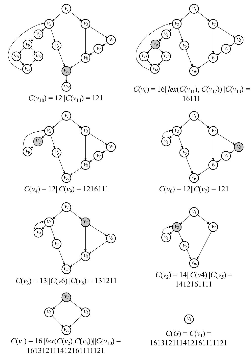
In order to define the code for a Dijkstra graph , we assign an integer, named , for each statement graph , a code for each vertex , and a code for each prime subgraph of a bottom-up contractile sequence of . The code of the graph is defined as being that of the source of . For a subset , the code of is the set of strings . Write whenever and is lexicographically not greater than .
| statement | ||
| graphs | ||
| trivial | 1 | |
| sequence | 2 | |
| if-then | 3 | |
| while | 4 | |
| repeat | 5 | |
| if-then-else | 6 | |
| -case |
Next, we describe how to obtain the actual codes. The types of the the different statement graphs are shown in the second column of Table 1. For a vertex , the code is initially set to 1. Subsequently, if becomes the source of a prime graph , the string is updated by implicitly assigning where is given by the third column of the table. Such an operation is called the expansion of . It follows that is written in terms of and the codes of the vertices of , and so on iteratively. A possible expansion of some other vertex could imply in an expansion of , and so iteratively. Observe that when is an if-then-else or a -case graph, we have chosen to place the codes of the out-neighbors of in lexicographic ordering. For the remaining statement graphs , the ordering of the codes of the out-neighbors of is also unique and implicitly imposed by . When all primes associated to have been expanded, has reached its final value,
5.1 The Isomorphism Algorithm
Next, we describe the actual formulation of the algortithm.
Let be a DG. Algorithm 2 constructs the encoding for .
An example is given in Figure 8.
5.2 Correctness and Complexity
Theorem 10
Let de Dijkstra graphs, and their codes, respectively. Then are isomorphic if and only if .
Proof
By hypothesis, are isomorphic. We show that it implies . Following the isomorphism algorithm, observe that the number of 1’s in the strings represents the number of vertices of , respectively, whereas each integer in the strings, represents the contraction of a prime subgraph. Furthermore, each prime subgraph , which is initially contained in the input graph , corresponds in , to a substring formed by the integer followed by one 1, if ; or two 1’s, if ; or three 1’s, if ; or 1’s, if ; respectively. Clearly, the same holds for the graph and its code . The proof is by induction on the number of contractions needed to reduce both and to a trivial vertex. By Theorem 6, is invariant and applies for both graphs and . If then both and are trivial graphs, and the theorem holds, since . When , assume that if and are isomorphic DG graphs which require less than contractions for reduction then . Furthermore, assume also by the induction hypothesis, that if are vertices of , corresponding to 1’s at the same relative positions in and , respectively, then , where is the isomorphism function between and . Now, consider the graphs and . Choose a prime subgraph of , and let . Let be a vertex of corresponding to by the isomorphism. Since , it follows that is the source of a prime subgraph of . Moreover . Consider the contractions and , leading to graphs and , respectively. Let and be the strings obtained from and , respectively by contracting the substrings corresponding to and , as above. That is, all the 1’s of and are compressed into the positions of and , respectively, while the integers and become 1, maitaining their original positions. It follows that and . By the induction hypothesis and the 1’s corresponding to and lie in the same relative positions in the strings. Consequently, by replacing the latter 1’s for the substrings which originally represented and , we conclude that indeed , and moreover the induction hypothesis is still verified. The converse is similar.
The corollaries below are direct consequences of Theorem 10.
Corollary 11
Let be a DG. The following affirmatives hold.
- 1.
There is a one-to-one correspondence between the 1’s of and the vertices of .
- 2.
The code of G is unique and is a representation of .
Corollary 12
Let be DGs and their corresponding codes, satisfying . Then an isomorphism function between and can be determined as follows. Let and correspond to 1’s at identical relative positions in and , respectively. Define .
Finally, consider the complexity of the isomorphism algorithm.
Lemma 13
Let be a Dijkstra graph, and its code. Then , where is the number of vertices of and the number of contractions needed to reduce it to a trivial vertex.
Proof
The encoding consists of exactly 1’s, together with elements of a multiset . We know that starts and ends with an 1, and it contains no two consecutive elements of . Therefore . When consists of the induced path , it follows , attaining the bound.
Theorem 14
The isomorphism algorithm terminates within time.
Proof
Recall that , by Lemma 7. The construction of a bottom-up contractile sequence requires steps. For each , following the isomorphism algorithm, can be constructed in time . We remark that lexicographic ordering takes linear time on the total length of the strings to be sorted. It follows that the algorithm requires no more than time to construct the code of .
6 Conclusions
The analysis of control flow graphs and different forms of structuring have been considered in various papers. To our knowledge, no full characterization and no recognition algorithm for control flow graphs of structured programs have been described before. There are some related classes for which characterizations and efficient recognition algorithms do exist, e.g. the classes of reducible graphs and D-charts. However, both contain and are much larger than Dijkstra graphs.
An important question solved in this paper is that of recognizing whether two control flow graphs (of structured programs) are syntactically equivalent, i.e., isomorphic. Such question fits in the area of code similarity analysis, with applications in clone detection, plagiarism and software forensics.
Since the establishment of structured programming, some new statements have been proposed to add to the original structures which forms the classical structured programming, enlarging the collection of allowed statements. Some of such relevant statements are depicted in Figures 9.
- (a)
break-while: Allows an early exit from a while statement;
- (b)
continue-while: Allows a while statement to proceed, after its original termination;
- (c)
break-repeat: Allows an early exit from a repeat statement;
- (d)
continue-repeat: Allows a repeat statement to proceed, after its original termination;
- (e)
divergent-if-then-else: A selection statement, similar to the standard if-then-else, except that the comparisons do not converge afterwords to a same point, but lead to disjoint structures. Note that the corresponding graph has no longer a (unique) sink.

In fact, the inclusion of some of the above additional control blocks in structured programming has been already predicted in some papers, as [17]. The basic ideas and techniques described in the present work can be generalized, so as to efficiently recognize graphs that incorporate the above statements, in addition to those of Dijkstra graphs. Similarly, for the isomorphism algorithm.
Acknowledgments
The authors are grateful to Victor Campos for the helpful discussions and comments during the French-Brazilian Workshop of Graphs and Optimizations, in Redonda, CE, Brazil, 2016. He pointed out the possibility of decreasing the complexity of the recognition algorithm from to .
References
- [1] F. E. Allen and J. Cocke, A program data flow analysis procedure, Comm. ACM 19 (1976), 137–147.
- [2] A. V. Aho and J. D. Ullman, Node listings for reducible flow graphs, J. of Computer and Systems Scien.ces 13 (1976) 286-299
- [3] L. M. S. Bento, D. R. Boccardo, R. C. S. Machado, V. G. Pereira de Sá and J. L. Szwarcfiter, Towards a provably resilient scheme for graph-based watermarking, Proc. 39th Intl. Workshop on Graph-Theoretic Concepts in Comp. Sci. (WG’13), LNCS 8165 (2013), 50–63.
- [4] C. Böhm and G. Jacopini, Flow diagrams, Turing machines and languages with only two formation rules, Comm. of the ACM 9 (1966), 366-371
- [5] N. Chapin and S. P. Denniston, Characteristics of a structured program, ACM SIGPLAN Notices 13 (1978), 36–45.
- [6] C. Collberg, S. Kobourov, E. Carter and C. Thomborson, Error-correcting graphs for software watermarking, 29th Workshop on Graph-Theoretic Concepts in Computer Science, (WG’03), Lecture Notes in Computer Science 2880 (2003), 156–167.
- [7] Collberg, C. and J. Nagra, Surreptitious Software: Obfuscation, Watermarking, and Tamperproofing for Software Protection. Addison Wesley (2010).
- [8] E. W. Dijkstra, Go-to statement considered harmful, Comm. ACM 11 (1968), 174–186.
- [9] O.-J. Dahl and C. A. Hoare, Hierarchical program structures, in Structured Programming, Academic Press, 1972, 175-220.
- [10] E. W. Dijkstra, Notes on Structured Programming, in Structured Programming (1972), 1–82, Acad. Press.
- [11] N.E.Fenton, R. W. Whitty and A. A. Kaposi, A generalized mathematical theory of structured programming, Theoretical Computer Science 36 (1985), 145-171
- [12] D. Harel, On folk theorems, Comm. of the ACM 23 (1980), 379-389
- [13] M. S. Hecht and J. D. Ullman, Flow graph reducibility, SIAM J. on Comp. 1 (1972), 188-202.
- [14] M. S. Hecht and J. D. Ullman, Characterizations of reducible flow graphs, J. ACM 21 (1974), 367–374.
- [15] P. Henderson and R. Snow, An experiment in structured programming, BIT 12 (1972), 38–53.
- [16] C. A. R. Hoare, Notes on data structuring, in Structured Programming, Academic Press, 1972, 83-174.
- [17] D. E. Knuth, Structured programming with go-to statements, ACM Comp. Surveys 6 (1974) 261–301.
- [18] D. E. Knuth and R. W. Floyd, Notes on avoinding ’go to’ statements, Inf. Proc. Let. 1 (1971), 23–31.
- [19] D. Knuth and J. L. Szwarcfiter, A structured program to generate all topological sort arrangements, Inf. Proc. Let. 2 (1974), 153–157.
- [20] S. R. Kosaroju,, Analysis of structured programs, J. of Computer and Systems Sciences 9 (1974) 232-255
- [21] D. Kozen and W.-L. D. Tseng, The Böhm-Jacopini Theorem is false, propositionally, Mathematics of Program Construction (MPC’ 08), CIRM, Marseille, France, Lecture Notes in Computer Science 5133 (2008), 177-192
- [22] T. J. McCabe, A complexity measure, IEEE Transactions on Software Engineering SE-2 (1976), 308-320.
- [23] P. Naur, ed. Report on the algorithmic language ALGOL 60, Comm. ACM 3 (1960), 299-314.
- [24] G. Oulsnam, Unravelling unstructured programs, The Computer Journal 25 (1982), 379-387.
- [25] R. E. Tarjan, Depth-first search and linear graph algorithms, SIAM J. Comp. 1 (1972), 146-160.
- [26] R. E. Tarjan, Finding dominators in directed graphs, SIAM J. Comp. 3 (1974), 62–89.
- [27] R. E. Tarjan, Testing flow graph reducibility, J. Comp. Sys. Sci. 9(1974), 355-365
- [28] N. Wirth, Program development by stepwise refinement, Comm. ACM 14 (1971), 221-227.
- [29] N. Wirth, The programming language PASCAL, Acta Informatica 1 (1971), 35-63.
- [30] N. Wirth, On the composition of well structured programs, ACM Comp. Surveys 6 (1974), 247-259.
- [31] M. H. Williams, Generating flow diagrams:the nature of unstructuredness, Computer Journal 20 (1977), 45-50
- [32] M. H. Williams, Flowchart schemata and the problem of nomenclature, Computer Journal 26 (1983), 270-276
- [33] M. H. Williams and H. L. Ossher, Conversion of unstructured flow diagrams to structured form Computer Journal 21 (1978), 101-107.
- [34] W. A. Wulf, A case against the Go-to, Proc. of the ACM Ann. Conf., 1972, 791-791.