Improving lognormal models for cosmological fields
Abstract
It is common practice in cosmology to model large-scale structure observables as lognormal random fields, and this approach has been successfully applied in the past to the matter density and weak lensing convergence fields separately. We argue that this approach has fundamental limitations which prevent its use for jointly modelling these two fields since the lognormal distribution’s shape can prevent certain correlations to be attainable. Given the need of ongoing and future large-scale structure surveys for fast joint simulations of clustering and weak lensing, we propose two ways of overcoming these limitations. The first approach slightly distorts the power spectra of the fields using one of two algorithms that minimises either the absolute or the fractional distortions. The second one is by obtaining more accurate convergence marginal distributions, for which we provide a fitting function, by integrating the lognormal density along the line of sight. The latter approach also provides a way to determine directly from theory the skewness of the convergence distribution and, therefore, the parameters for a lognormal fit. We present the public code Full-sky Lognormal Astro-fields Simulation Kit (flask) which can make tomographic realisations on the sphere of an arbitrary number of correlated lognormal or Gaussian random fields by applying either of the two proposed solutions, and show that it can create joint simulations of clustering and lensing with sub-per-cent accuracy over relevant angular scales and redshift ranges.
Keywords:
methods: statistical – gravitational lensing: weak – large-scale structure of Universe1 Introduction
One important concept used in cosmology is the random field, i.e. a field defined in space whose value at position is a random variable (Peebles, 1993, see). Examples of cosmological random fields are the matter density, matter velocity, CMB temperature fluctuations and polarisation, gravitational lensing convergence and shear fields. The full characterisation of a random field could be obtained with the specification of the joint probability density function (PDF) for .
A common and simple approximation used is to assume that is a multivariate Gaussian distribution. In this scenario, all marginal distributions – the PDFs for any particular – are Gaussians and is fully characterised by the mean vector (which in cosmology is generally zero) and the covariance matrix . Within this model it is possible to fully characterise (and therefore the random field) by constraining , and probably the simplest way to do this is to measure the field’s correlation function [which for a zero mean Gaussian field is actually equal to ] or its counterpart in Fourier or harmonic space. Further simplifications come from the statistical homogeneity of the Universe, which makes , and statistical isotropy, which leads to .
In some cases the multivariate Gaussian distribution is clearly not a good approximation. The matter density contrast , where is the density at position and its average, and the lensing convergence marginal distributions have hard lower limits which are not obeyed by Gaussian distributions and they show significant skewnesses and heavy tails at large values. A better approximation for is the multivariate shifted lognormal distribution (Coles & Jones, 1991; Taruya et al., 2002; Hilbert et al., 2011).
If a set of variables follows a multivariate lognormal distribution, this means that their logarithms follow a multivariate Gaussian distribution. The “shifted” term expresses simply that the distribution is translated around the space populated by the variables (see Sec. 2.1 for details). Even though this model introduces the shifts as extra parameters, they are in principle fixed by theory so a measurement of would also fully determine ; if the shifts are left to vary, an extra measurement like the marginals’ skewnesses are needed. This model has been extensively used for representing both the matter/galaxy densities (Coles & Jones, 1991; Chiang et al., 2013) and the convergence field (Taruya et al., 2002; Hilbert et al., 2011), and it was shown to provide a better approximation than the multivariate Gaussian, but it was also shown to depart from observational results and numerical simulations (Kofman et al., 1994; Bernardeau & Kofman, 1995; Kayo et al., 2001; Joachimi et al., 2011; Neyrinck, 2011; Seo et al., 2012). One of its main uses is to quickly simulate large-scale structure (LSS) observations to estimate measurement errors (Chiang et al., 2013; Alonso et al., 2015) and to test pipelines and estimators (Beutler et al., 2014, e.g.), all crucial steps for LSS surveys like the Dark Energy Survey11 1 http://www.darkenergysurvey.org (DES Collaboration, 2005, DES;), Euclid22 2 http://www.euclid-ec.org (Lumb et al., 2009), the Javalambre Physics of the accelerating universe Astrophysical Survey33 3 http://j-pas.org (Benitez et al., 2014, J-PAS;), the Large Synoptic Survey Telescope44 4 http://www.lsst.org (LSST collaboration, 2009, LSST;) and the Wide-field Infrared Survey Explorer55 5 http://wise.ssl.berkeley.edu (Wright, 2010, WISE;). Note that all these projects will cover large portions of the sky (from 5000 onwards) and many will reach redshifts of one or more.
In this paper we highlight an intrinsic limitation of lognormal variables mostly unknown by the astrophysical community that might irremediably prevent its use for modelling simultaneous measurements of galaxy density and weak lensing. This limitation comes from three combined facts: (a) the relation between two lognormal variables with different skewnesses is non-linear; (b) in cosmology the widely used measure for dependence between two variables is the Pearson correlation coefficient which works well only for linearly related variables; (c) the assumption that the density is lognormally distributed means that the convergence is not. We propose two different approaches to deal with this issue: distorting either the density and convergence fields’ auto- and cross-power spectra or the convergence marginal distributions (away from lognormals, making it in fact more realistic). We also present the open source code entitled Full-sky Lognormal Astro-fields Simulation Kit (flask)66 6 http://www.astro.iag.usp.br/~flask, capable of creating tomographic Gaussian and lognormal realisations of multiple correlated fields (multiple tracers, weak lensing convergence, etc.) on the full sky – using spherical coordinates – and of applying the two corrections suggested above.
This paper is organised as follows: an introduction to lognormal variables is given in Sec. 2.1, then in Sec. 2.2 we show how items (a) and (b) referred to above combine in a way to restrict the covariance matrices realisable by lognormal variables, while in Sec. 2.3 we analyse how this restriction translates into the harmonic space (i.e. the computation of angular power spectra). We then show in Sec. 3 that the density lognormality assumption leads to a non-lognormal distribution for the weak lensing convergence field, which might cause the lognormal model failure. Nevertheless, using this assumption we derive an analytical way of computing the convergence lognormal shift parameter which can be used to model the convergence field alone without resorting to ray-tracing measurements in -body simulations; in this section we also present a fitting function for the convergence distribution to better describe its deviations from the lognormal model. Sec. 4 details the two solutions to the modelling problem, already hinted by the previous sections: distorting the power spectra or using a theoretically consistent distribution for the convergence. Our code flask is described in Sec. 5, with an overview given in Sec. 5.1 and the details in Sec. 5.2. We conclude and summarise our work in Sec. 6.
2 Lognormal variables
2.1 Definition and properties
Given a set of variables following a multivariate Gaussian distribution with mean vector elements and covariance matrix elements , we call the random variables:
| (1) |
multivariate shifted lognormal variables, or lognormal variables for short in this paper. The parameters are called “shifts” by Hilbert et al. (2011) while are called “minimum values” by Taruya et al. (2002) and “thresholds” in the statistics literature (Crow & Shimizu, 1988, e.g.). A single lognormal variable is then fully described by three parameters: the shift (which acts as a location parameter), the associated Gaussian variable’s mean (which acts as a scaling parameter) and the associated Gaussian variable’s variance (which acts as a shape parameter). Since it possesses one extra parameter in comparison to Gaussian variables, it is more flexible than the latter. In fact, it tends to the Gaussian case as . Fig. 1 presents examples of the effects on the PDF of changing the distribution’s parameters.

The relations between the correlation function of lognormal variables and their parameters , and have been presented in the astrophysical literature for the case by Coles & Jones (1991) and for and by Hilbert et al. (2011). Here we generalise their results for multiple arbitrary shifts and expected values (i.e. statistical ensemble averages) .
The mean value of a lognormal variable can be obtained from Eq. 1 by expanding the exponential as an infinite series:
| (2) |
and remembering that the Gaussian central moments follow the relation
| (3) |
By inserting Eq. 3 into Eq. 2 and defining a new summation index , we get:
| (4) |
To derive the relation between the lognormal and associated Gaussian covariances and , we can write as a sum of zero-mean independent Gaussian variables , e.g. and such that . This allows us to treat the expectation value as a product of independent terms:
| (5) |
to which we can apply the same procedure used to derive Eq. 4, leading to:
| (6) |
| (7) |
where . Again the same method can be used to derive a relation for the three-point correlation function of lognormal variables:
| (8) |
By setting all indices in Eqs. 6 and 8 to the same value, we get relations for the variance and skewness of a lognormal variable:
| (9) |
| (10) |
The equation above can be inverted to obtain as a function of and ; although in principle Eq. 10 admits more than one as a solution, only one of them is real as the relation is monotonic. The shift parameter can then be written in terms of the variable’s mean, variance and skewness:
| (11) |
| (12) |
Once we have computed , we can get the remaining parameters of the lognormal distribution that possess the specified first three moments by inverting Eqs. 4 and 9:
| (13) |
| (14) |
This provides us with a method to fit a lognormal distribution to a dataset that exactly reproduces its mean, variance and skewness.
2.2 Intrinsic limitations of multivariate lognormals
To expose the fundamental limitations that lognormal variables face when modelling correlated data, consider a toy model consisting of only two variables. We can use Eq. 6 to build a relation between the Pearson correlation coefficients of the lognormal variables, , and that of their associated Gaussian variables, :
| (15) |
where and are the variances of the Gaussian variables and serve as shape parameters (which fully determines the skewness) of the lognormal distributions. The relation above is presented in Fig. 2 for different values of and , where it is possible to note that even perfectly correlated Gaussian variables () may not result in perfectly correlated lognormal variables. This happens because one cannot impose a linear relation between two variables and if their distributions have different shapes (e.g. different skewnesses) since such a relation only corresponds to shifting and rescaling one distribution to match the other (see Fig. 3). These limits on the Pearson correlation coefficient can be written in terms of the parameters of lognormal variables:
| (16) |
| (17) |
A more rigorous and general (but also complex) proof of the correlation limits above can be obtained from the use of copulas (Nelsen, 2006): any multivariate distribution can be described by a copula – a multidimensional function that alone specifies the variables’ inter-dependences – together with the one-dimensional marginal distributions of these variables. Copulas are useful because the dependence between the random variables becomes detached from their marginal distributions. The Fréchet–Hoeffding theorem states that all copulas are limited by specific functions and called lower and upper Fréchet–Hoeffding bounds. It is then possible to derive Eq. 16 by setting the two-dimensional copula to and and calculating the resulting correlations (Denuit & Dhaene, 2003, see also).


Suppose now that one ignores the limits above and assigns to a pair of lognormal variables a valid (i.e. positive-definite) covariance matrix but that violates Eq. 16. By using Eq. 7 one would find , which for a covariance matrix corresponds to being invalid (i.e. non-positive-definite).77 7 Assuming that the diagonal terms are positive. Since lognormal variables are associated to Gaussian variables by definition, the non-positive-definiteness of the Gaussian variables’ covariance matrix shows that such lognormal variables cannot exist. In other words, a covariance matrix for lognormal variables is only valid if both itself and its Gaussian counterpart are positive-definite.88 8 Since the relation between Gaussian variables is always linear, their Pearson correlation actually reflects the degree of dependence between them. This statement can be extended to covariance matrices of arbitrary size; this is important because, when dealing with more than two variables, the condition set by Eq. 16 is necessary but not sufficient.
As an example of what may happen in more complex cases, imagine there are three lognormal variables with and that follow the covariance matrix below on the left:
| (18) |
This positive-definite (and seemingly innocent) covariance matrix hides the fact that the dependence between the first variable and the two others is very strong (the maximum correlation allowed by the difference in the shape of their distributions is ) whereas the dependence between the last two variables is not strong enough to be compatible with the former (since they have the same shape, their maximum correlation is ). Indeed, the correlation matrix of the associated Gaussian variables (right-hand side of Eq. 18) is non-positive-definite.
The limitations over three or more lognormal variables appear even when the one-dimensional marginals are exactly the same. Fig. 4 shows that the Gaussian covariances serve as shape parameters for the multivariate lognormal distribution just as the Gaussian variances do due to the non-linearity of the transformation. The shape of the distribution can be such that projections on two-dimensional spaces might give the impression that tighter correlations are possible when they are not.

Another way to deduce the connection between lognormal variables and their Gaussian counterparts covariance matrix is the following:
- 1.
Fact: lognormal variables always have, by definition, Gaussian variables associated to them;
- 2.
Fact: any set of random variables must have a valid covariance matrix associated to it;
- 3.
Hypothesis: is a set of multivariate lognormal variables and it has the covariance matrix ;
- 4.
- 5.
If our final conclusion 5 is not true, our hypothesis 3 must be false, that is, either are not multivariate lognormal variables or they do not follow . Trying to enforce both at the same time would be like requesting two different angles from an equilateral triangle. Note that the relation between and depends on the full multi-dimensional PDF of so although it might not be a multivariate lognormal it can retain, in principle, marginal lognormal distributions.
2.3 Limitations in harmonic space
A collection of 3D isotropic random fields can be described by a set of angular correlation functions for fields and redshift slices specified by the indices and . These correlation functions can be expressed in terms of angular power spectra through the relations (Durrer, 2008):
| (19) |
| (20) |
where are Legendre polynomials.
If the fields in question follow lognormal distributions in real space, the relation between the angular power spectra and that describe the lognormal fields and their associated Gaussian counterparts, respectively, is
| (21) |
Although the relation above is not as direct as the one in real space (see Eq. 7), it takes advantage of isotropy to make each multipole independent of one another and reduce the dimensionality of the covariance matrices to the number of fields and redshift slices specified by and . In other words, for each we have an independent covariance matrix with elements .
It is difficult to derive analytically how the restriction described in Sec. 2.2 affects the relation between and : given it is local in real space, the relation becomes non-local in harmonic space, i.e. relates to a combination of with different ; moreover, the multipoles described by are not themselves lognormal. However, a highly correlated field in real space should be highly correlated in harmonic space as well and therefore the conditions set in Sec. 2.2 cannot be completely avoided. This is shown in Fig. 5.

To draw the shaded regions in Fig. 5 we first computed the convergence auto- and cross-power spectra for sources inside 0.1-wide top-hat redshift bins centred at and using class99 9 http://class-code.net (Blas et al., 2011; Dio et al., 2013) and a flat model. These were transformed to using Eq. 21 – implemented by flask – and obtained by Hilbert et al. (2011) using ray tracing through -body simulations. For each we built a covariance matrix which was tested for positive-definiteness. To probe the whole parameter space in Fig. 5 we repeated this process several times after rescaling the cross power spectrum and changing .
The final message of Fig. 5 is that the limitations described in Sec. 2.2 manifest themselves in harmonic space and can indeed prevent the realisation of multipoles of lognormal fields, showing in these cases that the proposed fields cannot exist. Moreover, this seems to be the only relevant process affecting the positive-definiteness of – at least in the simple example shown and aside from much smaller numerical errors.
3 Lognormal large-scale structure models
3.1 Quantifying the lognormal failure and distorting
We investigated if the limitations referred to in the previous section manifest themselves in the density and convergence fields. We described the projected matter density contrast inside redshift bins and the weak lensing convergence for sources inside those bins as multivariate lognormal variables that obey a set of with and inferred the model’s validity by checking if the matrices with elements given by Eq. 21 were positive-definite.
When a matrix turned out to be non-positive-definite, we quantified the degree of “non-positive-definiteness” by computing the fractional change in the matrix elements needed to make it positive-definite. For that we used a multi-dimensional gradient to minimise the sum of the absolute values of the negative eigenvalues: by computing the change in the negative eigenvalues given a small fractional change in each one of the matrix elements we found a preferential direction in this -dimensional space to distort the matrix and applied a small change in this direction; we repeated this process until all eigenvalues were positive. Another method to regularise a covariance matrix is to perform an eigendecomposition of the matrix [, where is a matrix formed by the eigenvectors of and is a diagonal matrix formed by eigenvalues] and set the negative eigenvalues to zero. However, this method results in minimal absolute rather than minimal fractional changes; more specifically, it is guaranteed to minimise the Frobenius norm – i.e. the matrix elements’ quadratic sum – of the difference between the original and regularised matrices (Higham, 1988). We confirmed that the fractional change obtained by our method is indeed smaller than the one obtained from the latter, and that they both result in fractional changes of similar magnitude for not too close to zero. Both regularisation methods can be performed by flask. The regularised can be transformed back into to give a set of angular power spectra that would not fail to represent lognormal fields.
High fractional changes are needed when trying to model both density and convergence as lognormal fields. Broadly speaking the amount of distortion required to make positive-definite increases with and with the number of redshift bins, and is higher for the non-linear power spectra computed by halofit (Smith et al., 2003; Takahashi et al., 2012) and when low-redshift bins are included: with the closest bin centred at , the required amount of change goes from () for 3 bins to () for 20 bins when using linear (non-linear) power spectra. Other parameters have a smaller impact on the fractional changes. As Fig. 6 shows, changes affect mainly the high multipoles and are much larger than the numerical precision expected for these operations (see below).

To ensure that the results presented in Fig. 6 were not caused by numerical inaccuracies, we used both class and camb sources1010 10 http://camb.info/sources (Challinor & Lewis, 2011) to generate the required under a variety of precision settings and performed the transformation described in Eq. 21 using two different methods under two different programming languages. Our main method (implemented in flask) was built in C and used the discrete Legendre transform coded in s2kit1111 11 http://www.cs.dartmouth.edu/~geelong/sphere (Kostelec et al., 2000) to go back and forth into harmonic space, while our second method used the functions legval and legfit in python’s numpy package. Fig. 7 shows that numerical fractional errors are expected to remain below . We also confirmed the behaviour of our results for Gaussian and top-hat redshift bins of different widths, with and without different contributions included in the matter density distribution (redshift space distortions, gravitational lensing, Integrated Sachs–Wolfe effect and gravitational redshift) and with and without non-linear structure given by halofit.

When considering matter density contrast or weak lensing convergence separately – i.e. when modelling one of these fields independently of the other – any need for regularising covariance matrices results in diminute fractional changes, of order , that in general affect low multipoles (). Such small deviations from positive-definiteness might be caused by numerical inaccuracies and, in any case, are too small to be detectable especially at low multipoles where cosmic variance is large. We verified that this pattern is maintained for different matter density contributions portfolio, for the linear and non-linear power spectra, for class and camb sources with different precision settings and for various redshift ranges and binning (we tested from 2 to 50 redshift bins in the range ). In fact, the class computation of density power spectra never resulted in non-positive-definite covariance matrices . As an example, Fig. 8 shows the four largest fractional differences between the original input and the regularised ones when modelling the convergence in 19 top-hat redshift bins of width in the range .

3.2 Density and convergence lognormality inconsistency
A model where both density and convergence are lognormal variables includes by definition an internal inconsistency due to the following connection between the two, which ends encoded in the power spectra: one can compute the convergence for galaxies at angular position and redshift by integrating the matter density contrast along the line of sight (LoS) (Bartelmann & Schneider, 2001, eq. 6.16):
| (22) |
| (23) |
where is called transverse comoving distance:
| (24) |
and is the comoving distance, given by
| (25) |
| (26) |
In these equations is the Hubble’s constant, is the speed of light, , and are the total matter, dark energy and curvature density parameters, respectively, and is the dark energy equation of state. From Eq. 22 we see that if each is drawn from a lognormal distribution then is a sum of (correlated) lognormal variables. However, in contrast with Gaussian variables, the sum of lognormal variables is not a lognormal variable itself (Fenton, 1960, see Figs. 10, 11 and 12 and). Following the reasoning presented in the end of Sec. 2.2, this internal inconsistency might be the cause for the lognormal model failure.
3.3 Modelling convergence alone as a lognormal field
Unfortunately, there is no closed expression for the PDF of a sum of lognormal variables; this is still an active field of study and several approximating formulas have been proposed (Fenton, 1960; Schwartz & Yeh, 1982; Lam & Le-Ngoc, 2007; Li et al., 2011). Nevertheless, assuming that the joint probability distribution for at different is a multivariate lognormal distribution – i.e. are drawn from a multivariate Gaussian distribution –, it is possible to compute ’s moments using the equations described in Appendix A.
Given that , we have as well. The convergence variance and skewness are:
| (27) |
| (28) |
respectively, where is the matter density contrast LoS correlation function. Eq. 27 does not provide any new information since the variance is already fixed by the convergence power spectrum. Eq. 28, however, puts a constraint over the convergence distribution’s shape; if one wants to approximate the convergence as a lognormal variable, it can be used in conjunction with Eq. 11 to specify the distribution’s shift parameter directly from theory. This is useful since previous methods for determining relied on computationally expensive ray tracing through -body simulations (Taruya et al., 2002; Hilbert et al., 2011, e.g.). Another alternative method for computing lensing PDFs is given by Kainulainen & Marra (2011).
To verify these conclusions numerically, we used flask to create 12.5 million lognormal realisations of the LoS matter density in 41 top-hat redshift bins of width in the range and to obtain the convergence at for each realisation using Eq. 22. We then measured the statistics of the convergence sample and compared with the values expected from theory. As Table 1 shows, they all match to 1% or better. Using Eqs. 11, 13 and 14 we can compute the parameters of the lognormal distribution that would satisfy such statistics; these parameters are shown in the bottom part of Table 1.
| Statistic | Numerical | Theory |
|---|---|---|
| Mean | 0 | |
| Std. Dev. | 0.02182 | 0.02189 |
| Skewness | 0.513 | 0.508 |
| Lognormal fit | ||
| -2.063 | -2.050 | |
| 0.1682 | 0.1665 | |
| 0.1288 | 0.1306 |
Fig. 9 shows that the theoretical parameters from Table 1 – chosen to reproduce the first three moments of the distribution – indeed provide a good fit for the convergence derived as a sum of correlated lognormal variables. The reproduction however is not perfect as can be seen in Fig. 10. A similar analysis was performed for two-dimensional distributions and the results are presented in Figs. 11 and 12, where we see that the disagreement between the simulated distribution and the lognormal model is larger for the convergence–convergence joint distribution. This is reasonable given that, in this case, both one-dimensional marginals were distorted away from the lognormal model. Therefore, we might expect that higher-dimensional convergence distributions will be even less well approximated by the multivariate lognormal model.


At this point it is important to stress that, since convergence is not strictly a lognormal variable, different methods of determining its shift parameter will result in different values. One possible method – which was implemented by Taruya et al. (2002) – is to set the shift parameter as the minimum attainable convergence; in a lognormal density model, this is clearly the convergence for the empty line of sight [Eq. 22 with ] which is hard to be extracted from simulations (or observations) given that these consist of finite samples. Another method (Hilbert et al., 2011, implemented by) is to perform a least-squares fit to the convergence PDF. Table 2 compares the values obtained from each method when applied to the convergence modelled as a sum of lognormal variables (density LoS integration) and as a lognormal variable itself. While for the lognormal case the methods agree and return the shift specified a priori (apart from the minimum value method which suffers from finite sampling), there is no agreement for the other case (which unfortunately is more realistic). This means that the lognormal approximation for the convergence field cannot reproduce every aspect of the distribution and choices have to be made: if one wants to reproduce the convergence skewness, the moment matching method should be used; if one wants to reproduce the PDF shape as close as possible, the least-squares method should be preferred; and so on.
| Method | Sum of lognormals | Lognormal |
|---|---|---|
| Empty LoS | 0.2115 | – |
| True value | – | 0.1300 |
| Moment matching | 0.1288 | 0.1306 |
| PDF least square | 0.1482 | 0.1310 |
| Min. value | 0.0858 | 0.0779 |
3.4 Quantifying the deviation from lognormal distribution
To better describe the shape of the convergence 1D marginal distributions obtained by lognormal density LoS integration we used the minimum method to fit the following formula to that PDF:
| (29) |
| (30) |
In the equations above, is a slightly modified version of the Gaussianization transformation (Schuhmann et al., 2016, that is, it transforms variables that follow more general distributions into Gaussian ones; ) when its parameters and are restricted to and .1212 12 In reality, the fitting was performed with unrestricted and , but the best fit remained in the and region. Given that the transformation is a piecewise function, we only show here the and sub-function. The more general PDF and the PDF of a Gaussian variable are related by a simple change of variables: , where is a Gaussian PDF.
The simulated data used were million convergences for sources at each of the redshifts specified in Table 3, convolved with Gaussian window functions of radius (standard deviation) 1.23 arcmin. These were produced by integrating the lognormal density simulated in 40 equal-width redshifts bins in the range (details of this procedure are given in Sec. 4). For each redshift, the convergences were distributed into 500 bins covering the full data range, but when fitting the function given by Eq. 29 we restricted our analysis to the range that does not include bins with zero counts. Together with this range, Table 3 presents for each redshift the parameters , , , and that best fit the convergence PDFs, along with the best-fit -value. In most cases, the -values indicate that the fits are quite good.
| -value | ||||||||
|---|---|---|---|---|---|---|---|---|
| 0.525 | -0.0164 | 0.105 | -0.001458 | 0.00690 | 31.034 | -1.383 | 0.040 | 0.002 |
| 0.575 | -0.0191 | 0.121 | -0.001516 | 0.00764 | 27.047 | -1.663 | 0.053 | 0.103 |
| 0.625 | -0.0213 | 0.117 | -0.001566 | 0.00837 | 23.974 | -1.998 | 0.069 | 0.052 |
| 0.675 | -0.0234 | 0.111 | -0.001609 | 0.00907 | 21.405 | -2.400 | 0.089 | 0.281 |
| 0.725 | -0.0257 | 0.123 | -0.001647 | 0.00976 | 19.019 | -2.748 | 0.111 | 0.425 |
| 0.775 | -0.0286 | 0.132 | -0.001680 | 0.01044 | 17.368 | -3.346 | 0.145 | 0.385 |
| 0.825 | -0.0315 | 0.125 | -0.001708 | 0.01109 | 15.864 | -4.070 | 0.188 | 0.231 |
| 0.875 | -0.0342 | 0.141 | -0.001734 | 0.01173 | 14.419 | -4.766 | 0.235 | 0.270 |
| 0.925 | -0.0361 | 0.139 | -0.001755 | 0.01235 | 13.412 | -6.209 | 0.322 | 0.648 |
| 0.975 | -0.0382 | 0.137 | -0.001772 | 0.01295 | 12.596 | -8.798 | 0.476 | 0.715 |
| 1.025 | -0.0409 | 0.147 | -0.001786 | 0.01354 | 12.060 | -16.499 | 0.922 | 0.074 |
| 1.075 | -0.0435 | 0.154 | -0.001799 | 0.01411 | 11.249 | -30.820 | 1.807 | 0.389 |
| 1.125 | -0.0461 | 0.141 | -0.001812 | 0.01466 | 10.055 | -30.820 | 1.935 | 0.172 |
| 1.175 | -0.0484 | 0.144 | -0.001823 | 0.01520 | 9.048 | -30.820 | 2.064 | 0.859 |
| 1.225 | -0.0501 | 0.151 | -0.001832 | 0.01573 | 8.194 | -30.820 | 2.196 | 0.161 |
| 1.275 | -0.0517 | 0.152 | -0.001841 | 0.01624 | 7.490 | -30.820 | 2.324 | 0.399 |
| 1.325 | -0.0535 | 0.151 | -0.001846 | 0.01673 | 6.670 | -30.820 | 2.460 | 0.356 |
| 1.375 | -0.0560 | 0.153 | -0.001851 | 0.01722 | 6.045 | -30.820 | 2.594 | 0.068 |
| 1.425 | -0.0584 | 0.172 | -0.001857 | 0.01769 | 5.447 | -30.820 | 2.726 | 0.098 |
| 1.475 | -0.0603 | 0.171 | -0.001859 | 0.01814 | 4.913 | -30.820 | 2.861 | 0.263 |
| 1.525 | -0.0617 | 0.161 | -0.001862 | 0.01859 | 4.426 | -30.820 | 2.998 | 0.060 |
| 1.575 | -0.0637 | 0.173 | -0.001863 | 0.01902 | 3.955 | -30.820 | 3.133 | 0.012 |
| 1.625 | -0.0652 | 0.155 | -0.001864 | 0.01945 | 3.642 | -30.820 | 3.272 | 0.001 |
| 1.675 | -0.0663 | 0.181 | -0.001864 | 0.01986 | 3.103 | -30.820 | 3.407 | 0.050 |
| 1.725 | -0.0672 | 0.186 | -0.001865 | 0.02027 | 2.721 | -30.820 | 3.543 | |
| 1.775 | -0.0685 | 0.169 | -0.001864 | 0.02066 | 2.393 | -30.820 | 3.681 | 0.003 |
| 1.825 | -0.0704 | 0.178 | -0.001864 | 0.02105 | 2.124 | -30.820 | 3.818 | 0.001 |
| 1.875 | -0.0725 | 0.179 | -0.001863 | 0.02143 | 1.798 | -30.820 | 3.954 | |
| 1.925 | -0.0747 | 0.166 | -0.001862 | 0.02180 | 1.416 | -30.820 | 4.088 | 0.017 |
| 1.975 | -0.0768 | 0.191 | -0.001862 | 0.02216 | 0.972 | -30.820 | 4.221 | 0.058 |
| 2.025 | -0.0788 | 0.187 | -0.001860 | 0.02251 | 0.509 | -30.820 | 4.358 | 0.022 |
As the redshift increases, the number of density bins that get summed into the convergence increases and its distribution gets closer to a Gaussian due to the central limit theorem, thus making the distribution less complex and requiring less parameters. This is manifested by the strong correlation between and that grows with redshift up to a point where they diverge and the fits get unstable. To avoid this issue, for redshift 1.075 onwards we fixed at the best-fitting value obtained at that redshift. The parameters from Table 3 are also presented in Fig. 13. The resulting for various redshifts are shown in Fig. 14.


4 The line-of-sight integration solution
The limitations for simulating correlated density and convergence presented in Sec. 3.1 can be circumvented in three ways. First, by simulating Gaussian instead of lognormal fields; as explained in Sec. 2.2, Gaussian variables are less limited in terms of valid covariance matrices than lognormal ones (as a trade-off, however, one loses the skewness and minimum boundary of the lognormal distribution). A second option is to distort the input power spectra so they produce positive-definite covariance matrices; once you have a valid covariance matrix for the associated Gaussian multipoles, the lognormal simulation can proceed without further issues. This is acceptable if the application intended for the simulations does not require the input s to be linked to a particular cosmological model or if the fractional changes applied to the input s are within the precision tolerance. The third option is to generate an only-density lognormal simulation and obtain the convergence by performing an approximated LoS integration through a weighted Riemann sum of the simulated densities in the redshift bins; as presented in Sec. 3.1, density realisations are not plagued by lognormal limitations.
As shown in Figs. 9 to 12, such integration leads to a convergence field that follows a distribution different from the lognormal (although fairly similar). To test if such a convergence field follows the expected statistics, we created 1000 full-sky simulations of the density field in 40 contiguous redshift bins of width , spanning the range , and computed the convergence by approximating the integral in Eq. 22 by a Riemann sum. We approximated the continuous density contrast by its average inside redshift bins (which already is the class output) and the kernel by its average inside the same bins :
| (31) |
We then recovered the power spectra from the convergence field computed as above and compared with the class output. It is worth noting that the effects of such approximation can be predicted from , the spectra for the average density contrasts at redshift bins centred at and , computed by class. The power spectra expected for convergence at redshifts and , and for density contrast at redshift and convergence at redshift , are:
| (32) |
| (33) |
A representative set of the results of this comparison is shown in Fig. 15. All analysed power spectra in the range and for succeed in reproducing the theoretical ones computed by class with a 3% precision (we did not study the spectra for which the density is at higher redshift than the convergence since these are very small); in fact, the convergence–convergence power spectra in this redshift range all agree to class s at 1% all the way down to or better.

One thing that can be seen in Fig. 15 is that the agreement is worse at lower redshifts. This happens for two reasons: first, the number of density bins used to compute the convergence is smaller (10 for against 40 for ), rendering a coarser integral approximation; secondly, the truncation of the integral at instead of at (class could not compute power spectra for bins centred at ) is more relevant for lower redshifts, thus producing a systematic power loss. We can also see that the agreement is worse for lower multipoles. This happens because is more sharply peaked in this case and therefore the approximation of the integral by a sum is less accurate.
Another aspect worth noting in Fig. 15 is that the density–convergence power spectra are well recovered with a precision better that 1% down to in most cases, the exception being when the density redshift bin is very close to the convergence redshift. This might not be an issue for high redshifts where, as shown by the large error bars, such measurements are quite difficult to be performed, but at lower redshifts it can present up to 3% deviations at and even larger ones at lower multipoles. Part of the problem can be accounted by the precision of class s: the power spectra used to simulate the density fields have to be well tuned with the convergence spectra used as . Moreover, the outcome of Eq. 33 refers to the average density inside a top-hat bin and the convergence at an exact redshift , something that cannot be computed by class; the comparison was made with the convergence in a top-hat redshift bin of width centred at the border of the last density bin used in the integration.
Finally, Fig. 15 shows that the theoretical prediction from Eqs. 32 and 33, depicted by the red lines, works excellently. Thus, if the intended application for the simulations requires convergence fields that accurately follow a fiducial but otherwise can deviate from a specific cosmological model, this method can be very powerful since comparisons can be made to these predictions.
5 FLASK code description
5.1 Overview
The purpose of flask is to generate two- or three-dimensional random realisations of astrophysical fields such as matter, arbitrary tracer densities, weak lensing convergence and shear in a correlated way, that is, all simulated fields (e.g. multiple tracers and weak lensing) are connected through the same realisation and therefore follow the expected internal cross-correlations provided as input. According to the user’s choice, the realisations can follow either a multivariate Gaussian distribution or a multivariate lognormal distribution in which case each field’s one-dimensional marginal distribution is lognormal (note that mixed Gaussian and lognormal marginals can also be generated since the Gaussian case can be described as a special lognormal case when the field’s skewness is zero). In comparison to the Gaussian, the lognormal distribution is a better approximation to matter and tracer densities and to the lensing convergence; it also does not lead to nonphysical values such as negative densities.
Another flask feature is that the realisations are created on the full sky using spherical geometry: the observer is positioned in the centre of the simulation and the universe is discretized along the LoS into spherical shells around the observer of arbitrary thickness (like an onion) with the slices being themselves discretized into a fixed number of aligned pixels (see Fig. 16). Such geometry allows for easy implementation of effects such as evolution with redshift, redshift space distortions and survey selection functions. Moreover, it is well matched for upcoming large area surveys than box-shaped simulations.

The goal of flask is to create the full-sky lognormal simulations quickly. Its power spectrum realisation approach and its implementation in C++ using OpenMP allows it to generate, for instance, 40 full-sky redshift slices of correlated convergence and density fields, each with million pixels (, which permits analysis to be made up to multipoles around ), in 10 minutes using a 16 core computer. This redshift and angular resolution suffices to create full-size mock catalogues for photometric large-scale structure surveys, such as those planned by Euclid and LSST, with cosmological signals known to the per-cent level. Another relevant aspect of the approach adopted by flask is that the statistical properties of the fields (i.e. their power spectra and distributions) are defined a priori and obeyed by construction apart from discretization and truncation inaccuracies that vanish in the limit of infinite resolution. This can be an important advantage for certain applications like verifying power spectrum and correlation function estimators, evaluating their covariance matrices and testing the effects of systematics and statistical fluctuations on these measurements. On the down side, the fact that all statistical properties are set by the multivariate lognormal model means that the code cannot produce anything different from that (although there is the option to model the convergence as a sum of correlated lognormal variables): three-point functions, for instance, are bound to behave according to the model and might not give a realistic representation of the data; for such applications one might need -body simulations (Fosalba et al., 2008, e.g. following).
After generating the fields [which might already include redshift space distortions, magnification bias and intrinsic alignments if these were included in the input power spectra – see Kirk et al. (2010); Challinor & Lewis (2011); Blas et al. (2011); Dio et al. (2013)], flask can: apply survey selection functions (that can be different for different tracers and can be separable or not into radial and angular parts), Poisson sample tracers from their density fields, compute shear and ellipticities and introduce Gaussian noise in the latter. The final results can be output in the form of a source catalogue. Appendix B presents an example of flask usage and output.
5.2 Details
5.2.1 Input
Flask is run by calling it on a terminal followed by a configuration file containing all specifications needed – which can also be overridden through the command line. Besides a keyword setting the type of simulation to be performed – Gaussian, lognormal or homogeneous (i.e. Poisson sampling from density fields containing no structure) –, two inputs described in the configuration file fully specify all statistical properties of the fields: a file containing a table of fields’ means, shifts and redshift ranges and a set of angular auto and cross power spectra for all fields at all redshift slices that must be provided by the user (the indices and cycle both through fields and redshift slices). These s can be calculated by public codes such as class (Blas et al., 2011; Dio et al., 2013), by camb sources (Challinor & Lewis, 2011) or by any other routine. In order to fix the fields’ properties, all cross-correlations have to be specified [there is an option to treat missing s as zero, that is, the field/redshift is uncorrelated with the field/redshift ]. For instance, fields described in redshift slices require a total of s to be fully specified. Each field can be simulated in a different number of redshift slices which can have different ranges as well.
5.2.2 Obtaining the associated Gaussian power spectra
The process of simulating a lognormal field involves first generating a Gaussian one and exponentiating it afterwards. To associate the statistical properties of the Gaussian to the lognormal field using Eq. 7 we assume statistical homogeneity and isotropy and that the field value at each point in space is a random variable. Since Eq. 7 is local, the correlation functions of the lognormal and Gaussian fields and have the same form as that equation:
| (34) |
Even though specify a covariance matrix for the field in all points in space that could be used to generate correlated Gaussian variables, in practice this approach is impossible due to its size. A more economical approach is to go to harmonic space since isotropy leads to independent multipoles. The relations between the correlation function and the power spectrum are given by Eqs. 19 and 20. To obtain the angular power spectra for the Gaussian fields we: (i) transform the input to real space using Eq. 20; (ii) compute using Eq. 34; and (iii) go back to harmonic space with Eq. 19. In practice the transformations to and from harmonic space are performed using the discrete Legendre transform routines implemented in s2kit1313 13 http://www.cs.dartmouth.edu/~geelong/sphere (Kostelec et al., 2000). For Gaussian realisations, this transformation is skipped and the input power spectra are directly used to generate the multipoles; in other words, in this case flask simply sets .
It is interesting and important to note that since the relation between lognormal and Gaussian fields and is local in real space, it is non-local in harmonic space, i.e. each multipole of the lognormal field depends on a mix of the Gaussian multipoles. This can be demonstrated through a series expansion of the exponential:
| (35) |
We can expand and in spherical harmonics:
| (36) |
and show that the contribution of the last written term on the right-hand side of Eq. 35 to the multipole of the lognormal field is:
| (37) |
where are Wigner 3- symbols. These can be non-zero if and , which shows that can get contributions from with (see Fig. 17). The practical consequence of such non-locality is that if one wants to accurately simulate lognormal fields up to a bandlimit , it is necessary to generate Gaussian multipoles up to . This fact is a general characteristic of lognormal fields and does not depend on the chosen transform (e.g. an analogous relation exists for Fourier transforms). Fig. 18 shows an example of this effect for the density contrast angular power spectra at redshift for a model; the larger the non-Gaussianity, the larger the effect.


Lastly, the necessity of truncating the series in Eq. 20 at a finite introduces a hard bandlimit that translates into oscillations in . These oscillations can be minimised by increasing the series range to higher and/or by introducing a high- suppression in . Flask has the option of applying exponential suppressions and those that result from convolving the field with Gaussian and/or Healpix pixel window functions.
5.2.3 Generating correlated multipoles
The statistical isotropy of the simulations allows for each multipole with different and indices to be generated independently. However, multipoles with the same and but from different fields and/or redshift slices (hence different indices) might be correlated. To generate such correlated Gaussian multipoles, we construct a covariance matrix for each multipole using the values of as elements of that matrix. We then apply a Cholesky decomposition [using the GNU Scientific Library (GSL) routine1414 14 http://www.gnu.org/software/gsl] to the covariance matrix :
| (38) |
where are lower triangular matrices which can be used to generate the correlated Gaussian multipoles from a set of standard (zero mean and unit variance) independent Gaussian variables :
| (39) |
The computation of the expected value shows that indeed follow where are Kronecker deltas.
Non-positive-definite matrices (those with non-positive eigenvalues) cannot be decomposed as in Eq. 38; in fact, these are invalid covariance matrices in the sense that no set of variables can possibly have such covariances. Even though one can start with a set of s that, as expected, leads to a positive-definite matrix for each , the matrix obtained as described in Sec. 5.2.2 might not be positive-definite for two reasons: numerical errors and the fundamental limitation described in Sec. 2.3. While numerical errors are small enough such that a fractional change of in the s (a negligible change for most cosmological applications) is sufficient to solve the problem, the second reason might need significantly larger fractional changes; moreover, it cannot be overcome with more accurate computations or different simulation methods since it is intrinsic to lognormal variables.
For generic fields, flask can fix this problem by distorting the covariance matrices as little as possible so they become positive-definite. Unfortunately, there are different ways to quantify the distance between two matrices; therefore, two methods are provided: one is guaranteed to minimise the Frobenius norm (quadratic sum of the matrix elements) of the difference between the regularised matrix and the original one (Higham, 1988); and the other aims at applying the smallest fractional change possible to the matrix. The first one is quite fast since it simply performs an eigendecomposition of the matrix [, where is a matrix whose columns are eigenvectors of and is a diagonal matrix formed by eigenvalues] and then sets the negative eigenvalues to zero (or close to zero for numerical reasons).
The second method is an iterative one and therefore takes more time. For an matrix, it tries to obtain positive eigenvalues by applying successive fractional changes to its elements in the -dimensional direction of greatest change for the negative eigenvalues. In other words, it computes the gradient of the sum of the negative eigenvalues as a function of all matrix elements and follows it until all eigenvalues are positive. Although there is no rigorous proof that this method reaches the minimum fractional change required to make the matrix positive-definite, this is what can be expected from following the negative eigenvalues gradient and it indeed performs better in this sense than alternative methods like simply adding small values to the matrix diagonal or like the first one presented (however it is possible that the larger fractional changes produced by the first method might only affect uninteresting s with very low power).
5.2.4 Map generation
Once the multipoles for the zero mean Gaussian fields are generated, we build healpix maps from them using the alm2map healpix function.
If the goal is to generate Gaussian fields, no extra step is needed. However, if one wants to generate lognormal fields , we have to apply the following local transformation to the Gaussian maps :
| (40) |
| (41) |
where is the variance of the Gaussian field , given by
| (42) |
Although can also be directly related to the lognormal field variance (Eq. 13) – which in turn is related to by an equation identical to Eq. 42 – the fact that in practice we generate Gaussian multipoles in the strict range means that the lognormal field multipole range is not well defined (see Sec. 5.2.2), making such calculation more difficult.
The multipole mixing referred to in Sec. 5.2.2 also introduces the issue that while the Gaussian field is band limited to , the exponentiation via Eq. 40 excites modes beyond as Eq. 37 exemplifies. Such an increase in the bandlimit is analogous to what happens in trigonometric identities such as . This leads to the need of higher healpix map resolutions than would be expected from the Gaussian field bandlimit to avoid aliasing effects. An example of this is shown in Fig. 19, where we compare the original power spectrum with the ones reconstructed from full-sky lognormal maps with different resolutions, all generated from an associated Gaussian field with bandlimit . While the resolutions as small as are enough for the Gaussian field, we need to go to to get to one per cent precision on the lognormal field. Together with the need to simulate the Gaussian field up to higher multipoles than required, this makes lognormal field simulations more costly in terms of memory than Gaussian fields.

Since homogeneity and isotropy of the fields on a spherical shell manifest themselves in the harmonic space as multipole independence , one might ask if the multipole mixing that happens during exponentiation can break these symmetries by introducing correlations between different multipoles. Fortunately, this cannot happen since the transformation from a Gaussian to a lognormal field is local and homogeneous in real space over the spherical shell and as such cannot introduce a preferential location or direction. Nevertheless we verified the independence of the lognormal field multipoles by realising them 2000 times in the range and [since the field is real, ] and measuring all their correlations [a total of elements]. The off-diagonal terms ( with and ) only show random statistical fluctuations smaller than 5 per cent. This isotropy conservation means that the exponentiation process is a rotation (and possibly an isotropic dilation) in harmonic space.
5.2.5 Density line-of-sight integration
If a set of density maps were generated in contiguous redshift slices (of arbitrary thickness), flask can use them to compute a convergence field for sources located at each slice boundary up to the last one at redshift using the approximation described in Sec. 4. For these convergence fields to be accurate, the redshift slices should be reasonably thin and cover the redshift range . The power spectra expected to be followed by these convergence fields (e.g. the red curves in Fig. 15) can be computed by an auxiliary routine in flask.
5.2.6 Shear computation
Weak gravitational lensing caused by matter distributed along the LoS will distort the images of distant galaxies by bending the path travelled by the photons coming from them: if a photon comes from the true angular position , it might be observed at a different position . The distortion in the image can be described to first order by the partial derivatives of with respect to components, , which is parametrized by the three parameters (convergence), and (Bartelmann & Schneider, 2001, shear components;):
| (43) |
Both the shear distortion and the flux and apparent size magnification described by the convergence are caused by the same intervening matter, and the shear can be deduced from the convergence, whose angular power spectra should be provided by the user as input if one wants to generate shear fields (alternatively, the convergence can be computed from the density fields as presented in the previous section). The shear can be described as an expansion over spin-2 spherical harmonics (Zaldarriaga & Seljak, 1997, as in healpix convention):
| (44) |
According to Hu (2000), on the full sky the harmonic multipoles are related to the convergence ones by:
| (45) |
Therefore the process of computing the shear and involves first computing from . For Gaussian realisations, the latter are obtained directly as described in Sec. 5.2.3, whereas for lognormal realisations they have to be extracted from the lognormal healpix maps computed as described in Sec. 5.2.4. We then use the healpix function alm2map_spin to transform the shear and mode multipoles, and , into and . According to the healpix manual, and .
In the lognormal case, we must obtain from the maps using the map2alm_iter function (with one iteration), and this process can introduce noise in the shears if the map resolution is too low compared to the shear bandwidth . To avoid that, we recommend .
5.2.7 Noise and selection effects
Once the tracer density contrast fields are available, flask can apply the survey selection function (i.e. the expected observed density if the universe had no structure, provided by the user) to to get the expected observed density, used as the mean value of a Poisson distribution from which we will draw the actual observed tracer density :
| (46) |
The user has to provide a selection function for each one of the tracers (if there is more than one) and each selection function can be separable or not into angular and radial directions. For separable selection functions, the user must supply: a file describing the radial part as a table containing the redshifts and the expected number of observed tracers of that type per unit per unit redshift; and a healpix map describing the fractions of this number that are observed at each angular coordinate. The final selection function is the product of these two. In the case of non-separable selection functions, a different healpix map must be provided for each redshift slice, each one containing the expected number of observed tracers per unit per unit redshift.
5.2.8 Catalogue building and output
All quantities computed in the previous sections (from angular correlation functions in Sec. 5.2.2 to healpix maps of in Sec. 5.2.7) can be written to output files on request, along with other quantities like the s obtained from the regularised matrices described in Sec. 5.2.3 and the s recovered from full-sky maps described in Sec. 5.2.4. The final flask product and output is a catalogue of observed tracers that might contain the following columns, according to user request: angular position (using polar and azimuth angles or right ascension and declination, given in radians or degrees), redshift, tracer type, convergence, shear components, ellipticity components (see Eq. 47), and a few bookkeeping numbers.
Up to the catalogue creation step, all tracers inside a cell are associated with the cell’s angular position (given by the healpix map pixel centre position) and redshift (given by its redshift slice). During the catalogue creation process, each tracer in the cell gets a random angular position homogeneously sampled within the pixel boundaries and a random redshift sampled within its redshift slice according to an interpolation of the selection function such that, even if the simulated redshift slices are thick, the resulting radial distribution of tracers is smooth (no structure will be generated inside the slices, though). The ellipticities are computed using the equation (Bartelmann & Schneider, 2001):
| (47) |
where is the reduced shear and is the source intrinsic ellipticity, randomly drawn from a Gaussian distribution with variance set by the user. For introducing intrinsic alignment in the simulations, these have to be specified via the input power spectra.
6 Summary and conclusions
The lognormal modelling of large-scale structure (LSS) fields is an important tool for validating LSS data analysis, estimating covariance matrices and studying impact of noise, selection and systematic effects on the data. Current and future photometric LSS surveys require this modelling to be performed jointly for many observables, on the full sky and over a large redshift interval. In this paper we explained some of the obstacles faced by this task and described how the modelling can be performed accurately. We also presented a public code that can create such simulations for a wide range of field combinations.
We showed in Sec. 2.2 that lognormal variables cannot attain certain correlations or covariance matrices that would be, for instance, accessible to Gaussian variables. Although this is a known fact in the field of statistics, it remained unnoticed by the astrophysics community given it does not manifest itself when modelling density and convergence fields in an independent way, as was done so far. We then showed in Sec. 2.3 that these limitations are propagated to the harmonic space in a similar but smoothed out way, and that as a consequence of such limitations the covariance matrix of the associated Gaussian variables becomes non-positive-definite.
In Sec. 3.1 we presented a way of quantifying the amount of “non-positive-definiteness” by computing the fractional change required to make the covariance matrix positive-definite and showed that, when modelling both density and convergence as a multivariate lognormal field, the change required is much larger than the expected numerical errors, demonstrating that they are caused by intrinsic limitations in the model; therefore, better implementations of the same simulation process will not circumvent the problem. We verified in Sec. 3.2 that the multivariate lognormal model for both density and convergence is internally inconsistent as the density lognormality assumption leads to a non-lognormal distribution for the convergence. This is likely the reason why the lognormal model fails to result in valid covariance matrices for the associated Gaussian variables when modelling both fields together.
We must therefore look for alternative methods if we want to create correlated random realisations of density and lensing. In this paper, two solutions were proposed: distorting the density and convergence auto and cross power spectra (Sec. 3.1); or using non-lognormal convergence marginal distributions (Sec. 4), for which we provided a fitting function in Sec. 3.4. Given that the lognormal model works well for the density and that the convergence can be obtained from the former by line-of-sight (LoS) integration, changing the shape of the convergence distribution to that of a sum of correlated lognormals allows both fields to be jointly modelled (see Fig. 15). Another (less attractive) possibility is to use the multivariate Gaussian model for creating realisations of the joint density and convergence fields: since the sum of Gaussian variables is also Gaussian, this model does not include the internal inconsistencies seen above. This alternative, however, has been shown to lead to underestimations of the convergence measurements covariance matrix (Hilbert et al., 2011).
Other bold possibilities would be to: (a) try different marginal distributions for the convergence [e.g. Das & Ostriker (2006); Schuhmann et al. (2016) or different approximations to the sum of lognormal variables] or even for the density fields; or (b) try different copulas (Nelsen, 2006, note that the multivariate lognormal distribution corresponds to the Gaussian copula with lognormal marginals;). Compared to the multivariate lognormal distribution, both have the disadvantage that specifying the fields’ statistical properties – e.g. the power spectra – might not be as straightforward as in the lognormal case (it might not even be analytically possible). Moreover, a different copula would still lead to the same limits in the fields’ correlations described in Sec. 2.2 given that they are limited by the Fréchet–Hoeffding bounds.
When modelling the convergence as a lognormal field, its shift parameter (an additional parameter that specifies the minimum value of the lognormal distribution ) is not fixed by the convergence power spectra and has to be determined somehow. Given that the true convergence field is not lognormal, different methods of estimating the shift parameter return different values (see Table 2) that confer to the model different characteristics when compared to the real distribution. Using Eqs. 11 and 28, we provided a way to specify it directly from theory, without relying on ray-tracing simulations. In comparison to the method by Taruya et al. (2002), our method is more complex but it is built to reproduce the convergence skewness while the method of Taruya et al. (2002) reproduces the minimum value observed in a finite sample. Given the arbitrariness on how is set when modelling the convergence distribution, there is no reason to expect it to match the minimum value of the convergence (i.e. the one obtained in an empty LoS, ) unless the fit is specifically built to reproduce this value in detriment of other properties. This conclusion leads us to question the common interpretation that the difference between and is an indication that there are no empty lines of sight in the Universe.
Finally, we presented in Sec. 5 the public code flask1515 15 http://www.astro.iag.usp.br/~flask which is able to simulate an arbitrary number of correlated lognormal and Gaussian fields including multiple tracer densities, convergence and CMB radiation once their statistics are specified by an input power spectra set which can be computed by class or camb sources, for instance. In case the lognormal limitations prevent the realisation of the fields, flask can overcome these limitations by distorting the input power spectra or by computing the convergence through a density LoS integration. Effects such as redshift space distortions, evolution, galaxy intrinsic alignments and arbitrary biases can be introduced by inscribing their effects in the power spectra, while selection functions and noise can be applied by flask itself. The code adopts a tomographic approach on the full curved sky, thus making it ideal for large-area photometric surveys like DES, Euclid, J-PAS, LSST and WISE.
7 Acknowledgements
The authors would like to thank Dr. Sreekumar Balan and Prof. Laerte Sodré Jr. for useful discussions. This work was made possible by the financial support of FAPESP Brazilian funding agency. BJ acknowledges support by an STFC Ernest Rutherford Fellowship, grant reference ST/J004421/1.
Appendix A Sum of correlated lognormal variables
We are interested in the first three central moments of the distribution of which is a sum of lognormal variables weighted by :
| (48) |
They can all be easily computed from the one-, two- and three-point functions presented in Sec. 2.1:
| (49) |
| (50) |
| (51) |
Appendix B flask usage example
Flask is executed in the command line by calling it together with a configuration file:
flask sim-01.config
The configuration file specifies all settings using keywords followed by a colon. For instance, RNDSEED: 1243 specifies the random number generator seed and MAP_OUT: data/kappa-map-01.dat specifies an output file for a table of field values at all angular positions. Flask comes with an example configuration file that describes all keywords; these are also explained in detail in flask’s documentation.
All settings can be overridden by providing new values in the command line, e.g.:
flask example.config RNDSEED: 334 MAP_OUT: ./map-002.dat
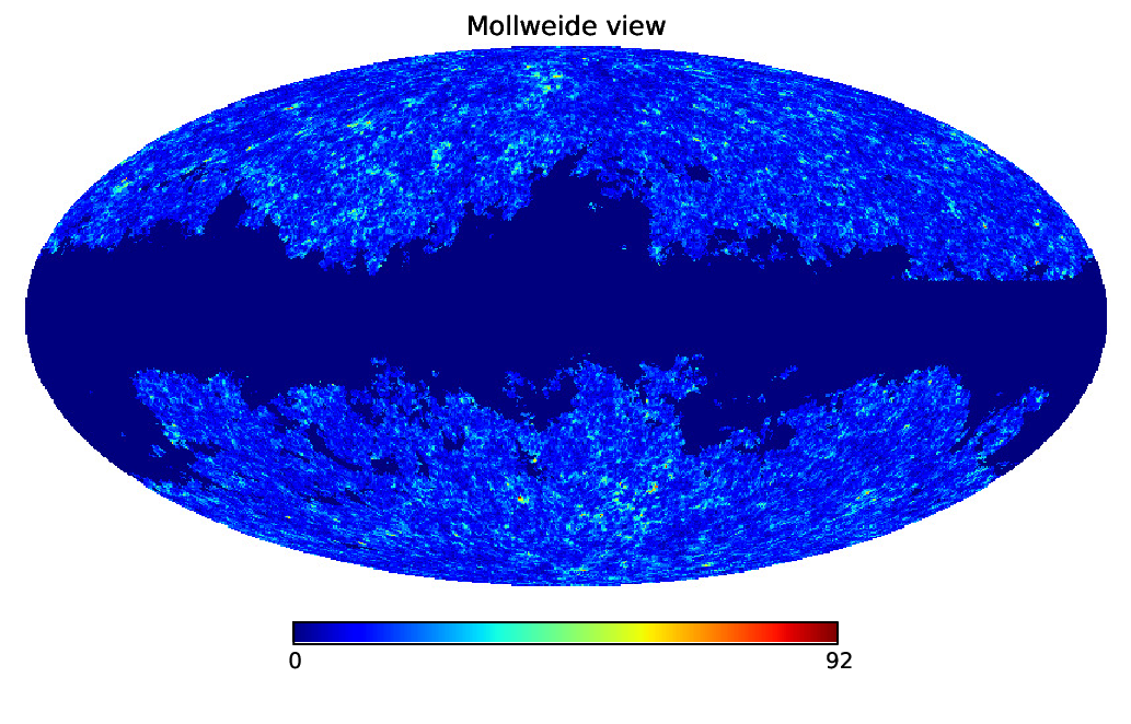
Among many possible outputs, the code can produce healpix maps of the generated fields. Fig. 20 shows a flask simulation of the WISE survey (under a model), consisting of galaxy counts following the survey selection function, including the Milky Way angular mask.
References
- Alonso et al. (2015) Alonso D., Salvador A. I., Sánchez F. J., Bilicki M., García-Bellido J., Sánchez E., 2015, MNRAS, 449, 670
- Bartelmann & Schneider (2001) Bartelmann M., Schneider P., 2001, Physics Reports, 340, 291
- Benitez et al. (2014) Benitez N., et al., 2014, arXiv pre-print, 1403.5237
- Bernardeau & Kofman (1995) Bernardeau F., Kofman L., 1995, ApJ, 443, 479
- Beutler et al. (2014) Beutler F., et al., 2014, MNRAS, 443, 1065
- Blas et al. (2011) Blas D., Lesgourgues J., Tram T., 2011, J. Cosmol. Astropart. Phys., 1107, 034
- Challinor & Lewis (2011) Challinor A., Lewis A., 2011, Phys. Rev. D, 84, 043516
- Chiang et al. (2013) Chiang C.-T., et al., 2013, J. Cosmol. Astropart. Phys., 2013, 030
- Coles & Jones (1991) Coles P., Jones B., 1991, MNRAS, 248, 248
- Crow & Shimizu (1988) Crow E. L., Shimizu K., 1988, Lognormal distributions: theory and applications. Marcel Dekker, Inc., New York, USA
- Das & Ostriker (2006) Das S., Ostriker J. P., 2006, ApJ, 645, 1
- Denuit & Dhaene (2003) Denuit M., Dhaene J., 2003, Belgian Actuarial Bulletin, 3, 22
- DES Collaboration (2005) DES Collaboration 2005, arXiv astro-ph, 0510346
- Dio et al. (2013) Dio E. D., Montanari F., Lesgourgues J., Durrer R., 2013, J. Cosmol. Astropart. Phys., 1311, 044
- Durrer (2008) Durrer R., 2008, The Cosmic Microwave Background. Cambridge University Press, Cambridge, UK
- Fenton (1960) Fenton L. F., 1960, IRE Transactions on Communication Systems, CS-8, 57
- Fosalba et al. (2008) Fosalba P., Gaztañaga E., Castander F. J., Manera M., 2008, MNRAS, 391, 435
- Higham (1988) Higham N. J., 1988, Linear Algebra and its Applications, 103, 103
- Hilbert et al. (2011) Hilbert S., Hartlap J., Schneider P., 2011, A&A, 536, A85
- Hu (2000) Hu W., 2000, Phys. Rev. D, 62, 043007
- Joachimi et al. (2011) Joachimi B., Taylor A. N., Kiessling A., 2011, MNRAS, 418, 145
- Kainulainen & Marra (2011) Kainulainen K., Marra V., 2011, Phys. Rev. D, 83, 023009
- Kayo et al. (2001) Kayo I., Taruya A., Suto Y., 2001, ApJ, 561, 22
- Kirk et al. (2010) Kirk D., Bridle S., Schneider M., 2010, MNRAS, 408, 1502
- Kofman et al. (1994) Kofman L., Bertschinger E., Gelb J. M., Nusser A., Dekel A., 1994, ApJ, 420, 44
- Kostelec et al. (2000) Kostelec P., Maslen D. K., Rockmore D. N., Healy D. J., 2000, J. Computational Physics, 162, 514
- Lam & Le-Ngoc (2007) Lam C. L. J., Le-Ngoc T., 2007, Wireless personal communications, 41, 179
- Li et al. (2011) Li X., Wu Z., Chakravarthy V. D., Wu Z., 2011, IEEE Transactions on Vehicular Technology, 60, 4040
- LSST collaboration (2009) LSST collaboration 2009, arXiv pre-print, 0912.0201
- Lumb et al. (2009) Lumb D., Duvet L., Laurijs R., Plate M. T., Sanz I. E., Criado G. S., 2009, Proceedings of the SPIE, 7436, 743604
- Nelsen (2006) Nelsen R. B., 2006, An Introduction to Copulas. Springer, New York, USA
- Neyrinck (2011) Neyrinck M., 2011, ApJ, 742, 91
- Peebles (1993) Peebles P. J. E., 1993, Principles of physical cosmology. Princeton University Press, Princeton, USA
- Schuhmann et al. (2016) Schuhmann R. L., Joachimi B., Peiris H. V., 2016, MNRAS, 459, 1916
- Schwartz & Yeh (1982) Schwartz S. C., Yeh Y. S., 1982, Bell System Technological Journal, 61, 1441
- Seo et al. (2012) Seo H.-J., Sato M., Takada M., Dodelson S., 2012, ApJ, 748, 57
- Smith et al. (2003) Smith R. E., et al., 2003, MNRAS, 341, 1311
- Takahashi et al. (2012) Takahashi R., Sato M., Nishimichi T., Taruya A., Oguri M., 2012, ApJ, 761, 152
- Taruya et al. (2002) Taruya A., Takada M., Hamana T., Kayo I., Futamase T., 2002, ApJ, 571, 638
- Wright (2010) Wright E. L., 2010, ApJ, 140, 1868
- Zaldarriaga & Seljak (1997) Zaldarriaga M., Seljak U., 1997, Phys. Rev. D, 55, 1830