∎
Symmetry breaking patterns of the 3-3-1 model at finite temperature
Abstract
We consider the minimal version of an extension of the standard electroweak model based on the gauge symmetry (the 3-3-1 model). We analyze the most general potential constructed from three scalars in the triplet representation of , whose neutral components develop nonzero vacuum expectation values, giving mass for all the model’s massive particles. For different choices of parameters, we obtain the particle spectrum for the two symmetry breaking scales: one where the group is broken down to and a lower scale similar to the standard model one. Within the considerations used, we show that the model encodes two first-order phase transitions, respecting the pattern of symmetry restoration. The last transition, corresponding to the standard electroweak one, is found to be very weak first-order, most likely turning second-order or a crossover in practice. However, the first transition in this model can be strongly first-order, which might happen at a temperature not too high above the second one. We determine the respective critical temperatures for symmetry restoration for the model.
Keywords:
3-3-1 model Symmetry patterns Phase transitionpacs
11.15.Ex 12.60.Fr 98.80.Cq1 Introduction
Extensive work has been dedicated to the study of the electroweak phase transition in the standard model (SM) as well as in many of its extensions. This interest is based for a large part on the possibility that it might explain the baryon asymmetry in the universe and that this asymmetry could be produced at around the scale of the electroweak symmetry breaking in the primordial hot Big Bang universe (for reviews see, e.g., Ref. [1]). One of the necessary conditions for a model to explain the baryon asymmetry of the universe is the presence of nonequilibrium effects. In a phase transition, this can be achieved if the transition is first-order and its strength is strong enough, in what is usually called a strong first-order phase transition. This condition is parameterized by the ratio , where is the value for the degenerate vacuum for the Higgs field at the critical temperature . A strong first-order phase transition is usually characterized by the condition . In the SM this condition cannot be achieved. Lattice Monte Carlo numerical simulations of the electroweak standard model [2, 3] have shown that there is an endpoint in the phase diagram of the model for a Higgs mass GeV, where the phase transition is weak first-order as the endpoint is approached from the left and the transition becomes a smooth crossover for larger Higgs masses. According to recent results from the Large Hadron Collider (LHC), from the current combined results from ATLAS and CMS experiments [4] have indicated the existence of a Higgs boson with a mass GeV. Thus, this gives no hope of achieving the necessary conditions for producing a baryon asymmetry in the context of the SM, since no significant departure from thermal equilibrium can be obtained during the phase transition dynamics. This is one of the motivations for looking for extensions of the SM and/or alternative models and the searches for new scalar particles at the LHC, aiming to reveal the ingredients needed for the strong first-order electroweak phase transition (EWPT), as required to produce the resulting observed baryon asymmetry.
On the theoretical side, some extensions of the SM have been analyzed and the kind of scalar was selected so as to remedy the SM shortcomings. These extensions used to enhance the SM are usually constructed with a scalar gauge singlet [5], a complex scalar or a scalar from supersymmetric degrees of freedom (in the context of supersymmetry extensions of the SM) [6]. On the other hand, there are alternative models, with a larger particle spectrum than the SM, that predict the existence of new gauge bosons and exotic quarks that acquire mass from their couplings to new scalar fields. In particular, in this paper, we are exploring the phenomenological aspects of an alternative to the SM based on the gauge symmetry, commonly known as the 3-3-1 model [7, 8]. In this model, the scalars are accommodated in a convenient fundamental representation of the symmetry group. From the electric charge operator one can select its model version. One particular version predicts the existence of new very massive gauge bosons and exotic quarks. In this work, we want to study and better understand the possible phase transition sequences associated with the symmetry breaking pattern in the 3-3-1 model and whether it can produce the necessary conditions required for generating a baryon asymmetry.
Let us outline some features of the model. Although at low energies the model has the same spectrum as the SM, it offers an explanation for basic open questions to the SM. In this model, the family replication problem is solved when considering that all three families are required for the anomaly cancellation procedure, resulting in the number of fermion families to have to be a multiple of the quark color number. Considering that the QCD asymptotic freedom condition is valid only if the number of families of quarks is less than five, one concludes that there are three generations. Another interesting feature of the minimal version of the model is the prediction of an upper bound for the Weinberg angle, which follows from a peculiar relation between new gauge boson masses.
The remainder of this paper is organized as follows. In Sec. 2, we present the main ingredients of the 3-3-1 model related to the spontaneous symmetry breaking (SSB). We give a brief exposition of its gauge, scalar and fermionic sectors, with a description of its spectrum of particles and its main motivations for us seeing it as an interesting and natural extension of the standard model. We also introduce the more general potential compatible with the given symmetry. In Sec. 3, we obtain the scalar spectrum after the SSB, explicitly showing the combination of the scalar fields transferring mass to the massive gauge bosons. In Sec. 4, we give the expression for the quantum and thermal corrections at the one-loop order to the tree-level potential for the model. In Sec. 5, we analyze and characterize the structure of symmetry breaking patterns in the model and we discuss our strategy for fixing the many parameters of the model so as to maximize the possibility of finding a strong first-order phase transition. We study the temperature-dependent one-loop corrected potential as a function of each value expectation value of the background fields and we graphically identify the temperature corresponding to symmetry restoration. From this analysis of the temperature dependence of the one-loop corrected model spectrum, we conclude that, in the 3-3-1 model, it shows two scales for first-order phase transition, with the final one, corresponding to the usual electroweak phase transition, as being very weak first-order, or probably second-order in practice. Finally, in Sec. 6, we give our concluding remarks.
2 The minimal version of the 3-3-1 model
In this section we recall the main characteristics of the minimal version of the 3-3-1 model [7, 8] related to the spontaneous symmetry breaking mechanism. We start by the definition of the electric charge operator,
| (1) |
where and are two of the eight generators () satisfying the algebra, is the unit matrix and denotes the charge. The minimal version of the model, used in this work, corresponds to the choice of the parameter .
To generate masses for all gauge and exotic quark fields through spontaneous symmetry breaking, three triplets of scalars, denoted by and , respectively, are needed,
| (2) |
The deviations of these fields from their ground state configuration and , are denoted by
| (3) |
where and are the deviations for the real and imaginary components of the fields, respectively, and we assume that the neutral part of each scalar develops a nonzero real vacuum expectation value (VEV): , and . We impose the consistency of the model with the SM phenomenology by adopting and , where gives the energy scale for the symmetry breaking , which is usually assumed to be at the TeV scale, for consistency with the current observations [9].
The gauge bosons, associated with the gauge symmetry of the model, consist of an octet () and a singlet , associated with . The model also predicts five vector bileptons: a single charged (), a doubly charged () and a new neutral gauge boson (), in addition to the charged standard model gauge bosons (), the neutral () and the photon (). These gauge bosons are defined as
| (4) | |||||
| (5) | |||||
| (6) | |||||
| (7) | |||||
| (8) | |||||
| (9) |
where and are the couplings defined in the covariant derivative of the scalar fields
| (10) |
The new gauge fields acquire mass at a high scale when the group breaks down to , by the scalar triplet, while the ordinary quarks and SM gauge bosons get acceptable masses at the next stage of SSB provided by the and triplets [10]. The resulting gauge boson tree-level field-dependent masses are given by
| (11) | |||
| (12) | |||
| (13) | |||
| (14) | |||
| (15) |
where , with [11] and , corresponding to the gauge coupling, given by .
Let us mention that, if the leptons are to get their masses at tree level within the usual Higgs mechanism, their Yukawa couplings would require a scalar () belonging to dimension six symmetric representation of the group [12]. We do not evaluate the tiny lepton masses generated by SSB because they give negligible contribution to the effective potential. Moreover, introducing a sextet scalar with a background neutral field developing a VEV, say , would modify the previous relation between the field vacuum expectation values with the Weinberg scale to , but keeping the adopted estimate .
The quark content is embedded in the extended group according to the multiplets and , where the SM quarks are and , whereas , and are the exotic heavy quarks needed to complete the fundamental representation. We define the background-field dependence of the top and exotic quark masses as
| (16) | |||
| (17) |
Finally, the scalar masses are obtained from the most general, gauge invariant and renormalizable potential [10] for the scalar fields and ,
| (18) | |||||
The tree-level potential, expressed in terms of the background fields , and , is
| (19) | |||||
By following a similar choice of parameters as used, e.g., in Refs. [10, 13], we fix the trilinear coupling as , where is a dimensionless constant. In particular, a common choice in the literature [10] is . The mass parameters determined by minimizing the tree-level potential in the vacuum, which gives
| (20) | |||||
| (21) | |||||
| (22) |
The potential (18) has a too large number of, in principle, free parameters, represented by the different possible magnitudes for the ten couplings, , , the vacuum expectation values for the triplet scalars, , and . Note that the constraint only tells us that these two VEVs are related to the same scale (the Weinberg scale), but does not fix the proportionality factor between them, i.e., we can parameterize and as and , where , but, in principle, with an arbitrary projection angle . Note that a natural choice is having , i.e., , however, in the literature there are some motivations for having , see, e.g., Refs. [14, 15]. Thus, we have a total of 12 free parameters for the scalar sector, composed of the ten couplings, the high energy scale associated with the first symmetry breaking and the projection angle . In the scalar sector we can still fix one of these parameters in terms of the others by making use of the Higgs mass . The stability of the potential only constrains the possible values for the couplings. In particular, should be positive for overall stability of the potential in the and directions, while the mixed couplings can in principle be negative.
We observe that the symmetry breaking scale for the electroweak theory down to is governed by . In addition, the lack of information as regards the individual roles of and fields in the SSB leads us to adopt, as already mentioned above, the polar parameterization and , such that in the vacuum, . Thus, after the second spontaneously symmetry breaking, where , it produces VEVs simultaneously for both and , but with an in principle arbitrary projection angle .
3 Mass spectrum for the scalars
The scalar sector for the 3-3-1 model can be divided in CP-even and CP-odd scalar sectors. The CP-even and CP-odd scalar sectors are further composed of a neutral scalar mass matrix, two single charged scalar and one double charged scalar matrices. For the CP-even scalar sector, the neutral scalar mass matrix is
| (23) |
In this sector one identifies two single charged scalars mass matrices, and , given, respectively, by
| (24) |
and
| (25) |
There is a double charge scalar mass matrix, given by
| (26) |
Next, we give the CP-odd scalar sector. The mass matrix of neutral scalars is given by
| (27) |
In this sector there are two mass matrices of single charged scalars, given, respectively, by
| (28) |
and
| (29) |
and a matrix for doubly charged CP-odd scalars,
| (30) |
The scalar and gauge boson masses depend on two VEVs ( and ), on the projection angle and on the ten couplings. We obtain the scalar masses by diagonalizing the corresponding and mass matrices given above.
We have in mind previous analyses [10, 13, 16] predicting that the neutral scalar CP-even sector must contain a low mass component corresponding to the SM Higgs particle . In addition, in this model, one expects two neutral scalars, and , in the CP-even sector. In the CP-odd sector, there is another neutral scalar, , along with two Goldstone bosons. For the charged states, one expects six massive scalars, and and another six Goldstone bosons. All the eight Goldstone bosons give mass to the massive gauge bosons, i.e., the SM gauge bosons and and the additional heavy bosons predicted by the present version of the model, , and . The four singly charged massive gauge fields ( and ), two doubly charged massive gauge fields () and two neutral massive gauge fields ( and ). These gauge fields have to obtain mass from the Higgs mechanism occurring at the electroweak scale and at the higher energy scale.
Our aim is to obtain the scalars, exotic quarks, and gauge boson masses using minimum arbitrariness. In order to fit the Higgs mass and the Goldstone fields with some set of parameters, one must respect the recent gauge boson mass lower limit determined from the upper limit on the ATLAS/LHC electron and muon production cross-section [9] (note also that there are also similar constrains for the from calculations of the muon magnetic moment [17]). By diagonalizing the matrix it is possible to respect the LHC constraint [9], TeV and to reproduce the SM Higgs mass. This in turn, from the expression for , Eq. (15), leads to a lower bound on the scale, TeV.
Once a given set of couplings are given, we obtain the whole scalar spectrum from the eigenvalues of the corresponding matrices calculated in the vacuum, , and . It results in nine scalars constructed from the real components of the fields. The SM Higgs is constructed from the combination . The other eight heavy scalars, namely and , are related to the and combinations, respectively, and are related to the combinations and , respectively, and , which is related to the combination. In the CP-odd sector, there is one heavy neutral , which is related to the imaginary part of the neutral field components. The gauge bosons and acquire their masses from the imaginary part of the fields in combinations , and , respectively. The neutral gauge bosons and get their masses from the imaginary part of the fields in the and combinations, respectively.
As already observed, the model has a too large number of free parameters, which makes it an almost impossible job to study the complete parameter region allowed. Since our objective in this work is to determine whether a strong first-order phase transition in the model is possible, our strategy for fixing the many couplings is then chosen so as to maximize this goal. For this purpose, we can borrow some of the lessons already learned when studying the phase transition in the SM and other extensions of it (see, e.g., Refs. [18, 19, 20] and references therein). To satisfy the usual criterion for a strong first-order phase transition, namely that the ratio of the field expectation value at the critical temperature and the critical temperature be larger than one, , we need, optimally, either a larger VEV at and/or a small . Typically is constrained by the scale, , which for us is rather large (recalling that TeV and and are constrained by the Weinberg scale. Since in general the VEV is given in terms of a combination of couplings and masses, , an ideally situation is to try to work with the smallest couplings possible. There is, however, a trade off. Too small couplings lead in general to a light particle spectrum, which for us is still limited by the scales and observational bounds (in particular, other scalars than the SM Higgs are expected to be sufficiently heavy for not being detected yet). The Higgs mass itself is the only limiting observational quantity we have in the scalar sector. Since the Higgs is a mass eigenvalue for the CP-even scalar neutral matrix, Eq. (23), it only (weakly) constrains the couplings , and .
In the analysis below, we fix GeV and work with four different sets of choices for couplings. Other possibilities can be shown to fall in one of these sets. In each of the sets used, we look for the ideal conditions for having a strong first-order phase transition, which, as mentioned above, favors the smallest choice of couplings in general. In all the sets we consider below, we found more convenient to vary the inter-couplings between the different fields, and , due to their relation to the SM Higgs mass (the other inter-couplings and , only appear on the heavy charged scalars and are unconstrained by the Higgs). We will consider the following four large sets of parameters:
- •
-
(a) Set I: The couplings , with , such that varied together with ;
- •
-
(b) Set II: The couplings , with , such that varied together with ;
- •
-
(c) Set III: The couplings , with , such that varied together with ;
- •
-
(d) Set IV: The couplings , with ,such that and , which are then varied.
For all sets we have fixed . This is motivated by the fact that determines the asymmetry of the potential in the direction and the more asymmetrical is the potential, the more we expect to have a stronger first-order phase transition. Note also that values of couplings larger than one can make us enter in a nonperturbative regime of parameters. We avoid this situation here, since we work only at the one-loop level for the effective potential for the model (see next section). In particular, we have explicitly checked that smaller values of always lead to weaker transitions. In addition, for each of the sets explained above, we have chosen to work with the higher energy scale with values , 4 and 5 TeV, satisfying the current constraints on the mass, as already mentioned. Likewise, for the projection angle , we have considered for each of the sets and values of the scale, the three values . Again, we have explicitly verified that larger asymmetries on the and directions are either disfavored, or there is a trade off, since as we decrease the projection in one direction, there is a compensation by the increase of the projection in the other direction (recalling again that and are constrained by the Weinberg scale ). Nonetheless, our analysis shows that the symmetrical case , i.e., , tends to be favored as far as the strength of the transition is concerned.
Each one of the parameters in the above four sets is then chosen so as to satisfy the Higgs mass GeV. The resulting relations between these couplings subject to this constraint are shown in Figs. 1(a), 1(b), 1(c) and 1(d).


We note from the results shown in Fig. 1 that for sets II, III and IV, there are always minimal values for the couplings. In the case of the set I, is a decreasing function of .
For illustration, the resulting scalar mass spectrum in each set is shown in the Table 1. For convenience, we show only the values at the minimal values of couplings in the case of the sets II, III and IV shown in Fig. 1. In the case of set I, the values of the masses are for , which we take as the limit for a ”perturbative” coupling. Note that exchanging by corresponds to change by . The dependence of on the set {} is the same as the dependence of on {}. As a consequence, the mass of the singly charged scalar for is the same as that for the double charged for . For completeness, the heavy gauge boson masses , and are shown in Table 2, for the cases of and TeV. Here again the dependence of on the set {} is the same as that of on the set {} and so we observe that for is equal to for , for any value.
| Set | |||||||
|---|---|---|---|---|---|---|---|
| 3.218 | 1.320 | 3.226 | 3.224 | 2.869 | 1.743 | ||
| I | 2.991 | 1.345 | 3.003 | 3.000 | 2.225 | 2.225 | |
| 3.218 | 1.320 | 3.226 | 3.224 | 1.743 | 2.869 | ||
| 3.225 | 1.694 | 3.226 | 3.224 | 2.920 | 1.825 | ||
| II | 3.003 | 1.762 | 3.003 | 3.001 | 2.301 | 2.301 | |
| 3.226 | 1.692 | 3.226 | 3.224 | 1.825 | 2.920 | ||
| 3.226 | 1.692 | 3.226 | 3.224 | 2.920 | 1.825 | ||
| III | 3.003 | 1.762 | 3.003 | 3.001 | 2.301 | 2.301 | |
| 3.225 | 1.694 | 3.226 | 3.224 | 1.825 | 2.920 | ||
| 3.223 | 1.148 | 3.226 | 3.224 | 2.852 | 1.715 | ||
| IV | 2.998 | 0.383 | 3.003 | 3.000 | 2.133 | 2.133 | |
| 3.223 | 1.148 | 3.226 | 3.224 | 1.715 | 2.852 |
| (TeV) | ||||
|---|---|---|---|---|
| 0.981 | 0.983 | |||
| 3 | 3.035 | 0.982 | 0.982 | |
| 0.983 | 0.981 | |||
| 1.307 | 1.309 | |||
| 4 | 4.047 | 1.308 | 1.308 | |
| 1.309 | 1.307 | |||
| 1.634 | 1.635 | |||
| 5 | 5.059 | 1.634 | 1.634 | |
| 1.635 | 1.634 |
In the next section we introduce the quantum and thermal corrections at the one-loop level for the effective potential in the 3-3-1 model and we analyze its temperature dependence, for the different set of parameters explained above, obtaining the symmetry restoration temperatures. As input, we use the SM values for the masses of the Higgs, quark top, gauge boson and : GeV, GeV, GeV and GeV. The exotic heavy quarks masses have been fixed as .
4 The one-loop effective potential for the 3-3-1 model
The effective potential is expressed as function of the background values for the scalars , and . It depends on the loop contributions from the gauge bosons, through their tree-level background-field-dependent masses, as well as those from fermions that can give a significant contribution to the effective potential, namely the top quark (t) and the three exotic heavy quarks (Q). Finally, we also have to add the contributions from the SM Higgs and from the nine scalars that become heavy in the vacuum after the first SSB. Besides, when choosing a gauge other than the unitary gauge, we have also to include the contributions from the eight Goldstone bosons. In this work, as is usual in the literature (see, e.g., Ref. [18] and references therein), we give the expression for the effective potential in the t’Hooft-Landau gauge.
The effective potential in terms of the background fields is expressed as
| (31) | |||||
where is the tree-level potential, Eq. (19), is the zero temperature (quantum) contribution for the one-loop effective potential, while is the finite temperature contribution at the one-loop level.
The one-loop quantum contribution is ultraviolet divergent and needs to be renormalized. In the cutoff regularization scheme with subtraction point chosen at the scalar vacuum expectation values (thus preserving the values of and ), is given by [18]
| (32) | |||||
where in Eq. (32) denotes the field degrees of freedom: The massive charged gauge bosons have (e.g., ), the neutral massive gauge bosons have (e.g., ), the heavy quarks have (e.g., the top and the three new exotic quarks ) and each of the neutral and charged scalars has . The last sum in Eq. (32) is over the Goldstone modes, each one contributing with . Finally, the masses and , with and , stand for the particle masses computed at the background and vacuum expectation values, respectively.


As an example, in Fig. 2 we show both the tree-level and the one-loop quantum corrected potentials in the case of , i.e., for , in the set II case of parameters explained in the previous section, taken at the minimal values of couplings. We have also considered the scale TeV. For convenience of presentation, we have subtracted from the potential the vacuum contribution at the origin (corresponding to an overall shift of the whole potential).
| (33) | |||||
where the functions and are defined as
| (34) |
and
| (35) |
The thermal bosonic one-loop integral (34), admits a high-temperature expansion, for (where ). It is given by [21]
| (36) | |||||
while the thermal fermionic one-loop integral (35), for , can likewise be expressed as
| (37) | |||||
In the above expressions, (and ), (or ) and is the Riemann -function.
| (38) |
It is interesting to find where the behavior of at low temperature matches its high-temperature expression. We find that the transition between the low- and high-temperature approximations occurs at for the bosonic thermal integral and at for the fermionic thermal integral. This is sometimes more useful for the numerical analysis than using the exact expressions (34) and (35). More explicitly, we find that a simple interpolation of the two regimes and a truncation in the high-temperature series in Eqs. (36) and (37), result in the following expressions:
| (39) | |||||
and
| (40) | |||||
which provide an excellent coverage of the exact integrals (34) and (35), respectively, in the whole region of high and low temperatures. It is crucial in the present work to pay particular attention to the specific approximation to be used in the effective potential, due to the large disparateness of the mass scales that the model has. At a given temperature, some particles may acquire a mass that is below the temperature and others might have a mass above the temperature, so we have different contributions to the effective potential at different temperatures. This is particularly important when we investigate the behavior of the effective potential in between the first transition and the final electroweak phase transition in the model.
In the next section we will present the results for the phase transition pattern in the 3-3-1 model for the different choices of the sets of parameters explained in Sec. 3.
5 Phase transition pattern in the 3-3-1 model
We can clearly identify the two transitions in the model as the temperature is lowered from values to values below the electroweak scale, . First, the higher symmetry group is broken down to the electroweak one, , at a temperature below the 3-3-1 scale . Then follows the usual electroweak phase transition, , at a temperature slightly below the Weinberg scale .


As an illustrative example of the phase transition related to the two SSB in the model, the temperature-dependent potential is shown in Fig. 3, considering the parameters of set II, with the couplings at its minimum values, for and TeV. In Fig. 3(a) we show the effective potential in the direction of . It shows the behavior of the effective potential with the temperature. For temperatures above the scale for the electroweak symmetry breaking, the temperature-dependent values and vanish (or, equivalently, ), since the electroweak symmetry is still in the symmetry restored phase. Figure 3(a) then shows that there is a temperature for which the potential displays degenerate minima with the one at the origin. Below this critical temperature the minimum with non-vanishing background field value becomes the global minimum and for temperatures slight above the critical value it is a local minimum, with the origin being the state of minimum energy. This corresponds to a background value for the field, , that changes discontinuously with the temperature, jumping from a value to a nonvanishing value at the temperature . This is the characteristic of a first-order phase transition (as opposite to a second-order phase transition, where the background field changes continuously with the temperature). The same behavior as seen in Fig. 3(a) is also shown in Fig. 3(b). In Fig. 3(b) we show the effective potential in the direction of (expressed in terms of ) for temperatures below the Weinberg scale . For these low values of temperature, we have that , i.e., the thermal expectation value for the field already approaches its vacuum value . All the heavy particles that make the extra particle spectrum of the 3-3-1 model acquire masses close to their vacuum values33 3 Note that the heavy particles have a dependence on the background fields and , which are, however, zero at and above the critical temperature . Thus, all heavy particles, with the exception of and the heavy quarks , which only depend on , will have values close but not exactly at their vacuum values. and they contribute little for the effective potential at this scale. Hence, the particle content dominating the effective potential at is essentially that of the standard model. Figure 3(b) shows that the final transition, corresponding to the standard model one, , happens at a temperature and it is of the type of a first-order phase transition.
In Table 3 we summarize the results for the two phase transitions in the 3-3-1 model, where we give the value for the critical temperatures for the two phase transitions in the model. The first one happens at a temperature and corresponding to the symmetry breaking , and the second transition corresponding to the electroweak symmetry breaking , happens at the temperature . Results are shown for the four sets of parameters considered in this work and for the three different projection angles (). We also show the ratio of the background field working as order parameter for each transition to the temperature at the critical point. As already mentioned, this is a useful measure of the ”strength” of the phase transition, as usually considered in the literature [1, 18] (for other alternative forms of characterizing the strength of the transition, particularly useful for weak first-order phase transitions, see, e.g., Refs. [22, 23]).
| Set | |||||
|---|---|---|---|---|---|
| 1.494 | 0.847 | 0.344 | 0.023 | ||
| I | 1.462 | 1.094 | 0.374 | 0.018 | |
| 1.494 | 0.847 | 0.344 | 0.023 | ||
| 1.701 | 0.800 | 0.205 | 0.080 | ||
| II | 1.830 | 0.525 | 0.204 | 0.080 | |
| 1.811 | 0.530 | 0.205 | 0.080 | ||
| 1.810 | 0.530 | 0.204 | 0.080 | ||
| III | 1.829 | 0.525 | 0.204 | 0.080 | |
| 1.698 | 0.807 | 0.204 | 0.080 | ||
| 1.295 | 1.060 | 0.205 | 0.079 | ||
| IV | 0.365 | 8.082 | 0.203 | 0.080 | |
| 1.295 | 1.060 | 0.205 | 0.079 |
In all cases shown in Table 3 the parameter sets are taken at their minimal values, shown in Fig. 1. We have explicitly verified that the values of specified correspond to the minimum possible critical temperature found within the range of couplings shown in Fig. 1. Changing the values of the couplings away from the minimum values satisfying the Higgs mass constraint always tend to increase the value of and, consequently, decrease the ratio . The same is true in general for , except for the case of set I, where we find that decreasing the value of the coupling , tends to decrease, thus increasing the ratio , but the minimum values of we have found are still limited by the minimum values shown in Table 3, and . This then implies that the results for the second transition, corresponding to , has values for the ratio that are always much smaller than one, which characterizes a very weak first-order, possibly second-order, phase transition. We have explicitly verified that by increasing the scale it causes very little changes to the second transition. This is consistent with the fact that the higher is , the sooner the heavier particles decouple from the SM electroweak spectrum. We also note that closer to the transition point it also known that self-energy corrections to the effective potential can make the transition even weaker [18, 24].
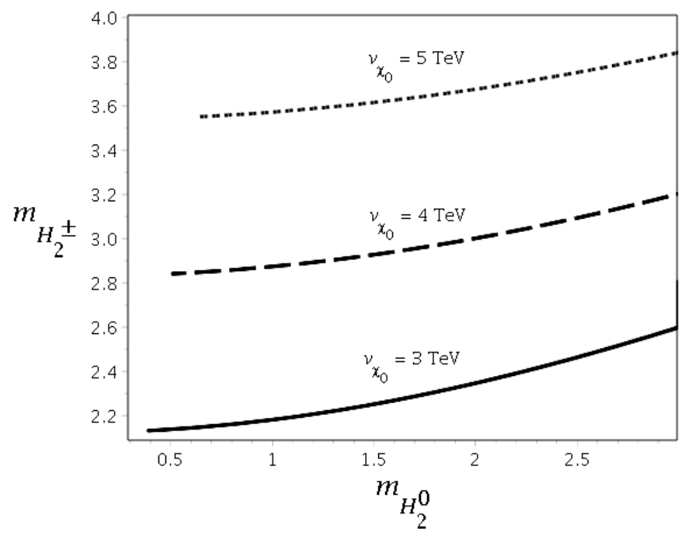
As far as the first transition is concerned, corresponding to , we find that it has a value for the critical temperature that increases proportionally to the scale , as we would expect on general grounds. The ratio tends to be closer to one, becoming larger when the scale increases. Among the different sets of parameters we have considered, the most favorable for producing a strong first-order phase transition, , is set IV, as explicitly noted from the values shown in Table 3. In particular, the case with , i.e., , is the one that is able to produce the strongest transition. Note, however, looking at the values for the scalar mass spectrum shown in Table 1, this is also the case that leads to the smallest mass for the Higgs like scalar particle , with a mass GeV. Increasing the scale this value of the mass also increases. For example, for TeV, we have GeV and GeV, with a ratio . In Fig. 4 we show the functional dependence for the masses of the lightest scalars after the standard model Higgs, i.e., for the scalars and (note that the double charged scalar is degenerate in mass with when ). The value of tends to increase (and consequently the ratio decreases) as we move from the smallest values of masses towards the largest values. For example, in the TeV, for TeV, we find that TeV and . Typically, we find that for all sets of parameters considered, within around . Note that this automatically implies a lower bound, , since the first transition must obviously occur at a temperature above the electroweak one.
6 Conclusions
In this work we have studied the symmetry breaking patterns of the 3-3-1 model at finite temperature. Making use of the minimal version of the model, we have first analyzed its scalar sector, which is constructed from three scalars in the triplet representation of and the most general renormalizable interactions that can be constructed with these fields. Despite the very large parameter space of the model, we have made an extensive analysis of the model making use of four large sets of parameters that give relations between the scalar couplings. This was done in such a way to maximize the possibility of finding a strong first-order phase transition on this model, motivated by its possible role in baryogenesis scenarios in extensions of the SM. This allowed us to make a systematic (though far from complete, it should be sufficiently representative for our purposes in this work) investigation the two symmetry transitions in the model, the and the standard electroweak one, .
On studying the temperature effects on the effective potential at the one-loop level, and within the approximations used, we have shown that the model encodes two first-order phase transitions. The last one, corresponding to the standard electroweak phase transition, , turns out to be always very weak, most likely turning into a second-order or a crossover in practice. For the first transition, corresponding to , we find that there are regions of parameters that can favor a strong first-order phase transition and, in particular, we have found that the critical temperature in this case is always close to the mass of the Higgs like scalar . This indicates that we can use the estimated value for the mass as a reasonable estimate for the temperature of transition .
Our results should be contrasted with some previous analyses of the phase transition performed in some variants of the 3-3-1 model done in Refs. [25, 26]. In the Ref. [25] the authors have used the so-called reduced minimal 3-3-1 model, while in Ref. [26] the economical 3-3-1 model was used. These models differ from the one we have used in the present work in the sense that they have a reduced number of couplings in the potential for only two scalar triplets interactions. The economical 3-3-1 model has a much richer leptonic content than the reduced minimal version and both versions exclude quarks with exotic electric charges. The SSB mechanism applied for determining how each ordinary or new gauge boson acquires the mass follows the same road as usual, The Goldstone bosons are identified, but no numerical value for the masses of the scalars have been shown. In Refs. [25, 26] the authors find parameter regimes where strong first-order phase transitions are found for both the and also for the transitions. This discrepancy as regards the strength of the predicted two step phase transition in these alternative models with our present results deserves an interpretation.
We believe that the most important source for the difference between our results and the previous ones come from the fact that in Refs. [25, 26] it was assumed that only one field direction would contribute at each transition, e.g., with in the first transition along the direction and with in the second transition along the direction. While this is basically true in the first case, where the temperature is sufficiently high to have , this is not the case for the second transition. As we have explained in Sec. 5, in the first transition the electroweak phase would still be in its symmetry restored phase for temperatures , thus . However, for the second transition, the temperature is already low enough, , so that and all the heavy particles that make the extra particle spectrum of the 3-3-1 model acquire masses close to their vacuum values decoupling from the particle spectrum (e.g., their temperature-dependent contributions to the effective potential become all Boltzmann suppressed). The particle content at these low values of the temperature is then dominated essentially by that of the standard model. As such, we expect the results not to differ strongly from the ones known for the phase transition in the standard model. That the heavy mass particles of the 3-3-1 model contributes little at the electroweak phase transition is confirmed by the results. We have found in all cases of sets of parameters considered here that the critical temperature , as well the ratio , are very weakly dependent on the scale , which controls the masses of the heavy particles.
Our results show that using the parameter set IV, in particular for , can lead to a very low critical temperature for the first transition. In particular, we have obtained the result that, for all parameters studied, within around . This result and the possibility of having a critical temperature not too high above that for the EWPT, , are deserving of further analysis in the future and may have for this model important implications as regards astroparticle physics and cosmology.
Acknowledgements.
R.O.R is partially supported by research grants from Conselho Nacional de Desenvolvimento Científico e Tecnológico (CNPq) and Fundação Carlos Chagas Filho de Amparo à Pesquisa do Estado do Rio de Janeiro (FAPERJ).References
- (1) A. G. Cohen, D. B. Kaplan and A. E. Nelson, Ann. Rev. Nucl. Part. Sci. 43, 27 (1993); M. Trodden, Rev. Mod. Phys. 71, 1463 (1999); A. Riotto and M. Trodden, Ann. Rev. Nucl. Part. Sci. 49, 35 (1999).
- (2) K. Kajantie, M. Laine, K. Rummukainen and M. E. Shaposhnikov, Nucl. Phys. B 466, 189 (1996); K. Kajantie, M. Laine, K. Rummukainen and M. E. Shaposhnikov, Phys. Rev. Lett. 77, 2887 (1996).
- (3) F. Csikor, Z. Fodor and J. Heitger, Phys. Rev. Lett. 82, 21 (1999).
- (4) G. Aad et al. [ATLAS and CMS Collaborations], Phys. Rev. Lett. 114, 191803 (2015).
- (5) J. McDonald, Phys. Lett. B 323, 339 (1994).
- (6) J. R. Espinosa, M. Quiros and F. Zwirner, Phys. Lett. B 307, 106 (1993).
- (7) F. Pisano and V. Pleitez, Phys. Rev. D 46, 410 (1992).
- (8) P. H. Frampton, Phys. Rev. Lett. 69, 2889. (1992)
- (9) C. Salazar, R. H. Benavides, W. A. Ponce and E. Rojas, JHEP 1507, 096 (2015).
- (10) M. D. Tonasse, Phys. Lett. B 381, 191 (1996).
- (11) K. A. Olive et al. [Particle Data Group Collaboration], Chin. Phys. C 38, 090001 (2014).
- (12) R. Foot, O. F. Hernandez, F. Pisano and V. Pleitez, Phys. Rev. D 47, 4158 (1993).
- (13) A. Alves, E. Ramirez Barreto, A. G. Dias, C. A. de S.Pires, F. S. Queiroz and P. S. Rodrigues da Silva, Phys. Rev. D 84, 115004 (2011).
- (14) A. C. B. Machado, J. C. Montero and V. Pleitez, Phys. Rev. D 88, no. 11, 113002 (2013).
- (15) H. Okada, N. Okada, Y. Orikasa and K. Yagyu, arXiv:1604.01948 [hep-ph].
- (16) M. B. Tully and G. C. Joshi, Int. J. Mod. Phys. A 18, 1573 (2003).
- (17) C. Kelso, H. N. Long, R. Martinez and F. S. Queiroz, Phys. Rev. D 90, 113011 (2014).
- (18) J. R. Espinosa, M. Quiros and F. Zwirner, Phys. Lett. B 314, 206 (1993).
- (19) S. W. Ham, Y. S. Jeong and S. K. Oh, J. Phys. G 31, 857 (2005).
- (20) A. Ahriche, Phys. Rev. D 75, 083522 (2007).
- (21) J. I. Kapusta and C. Gale, Finite-Temperature Field Theory: Principles and Applications, (Cambridge University Press, Cambridge, England, 2006).
- (22) M. Gleiser and R. O. Ramos, Phys. Lett. B 300, 271 (1993).
- (23) R. O. Ramos, Phys. Rev. D 54, 4770 (1996).
- (24) M. E. Carrington, Phys. Rev. D 45, 2933 (1992).
- (25) V. Q. Phong, V. T. Van and H. N. Long, Phys. Rev. D 88, 096009 (2013).
- (26) V. Q. Phong, H. N. Long, V. T. Van and L. H. Minh, Eur. Phys. J. C 75, 342 (2015).