Joint Scheduling and Power-Control for Delay Guarantees in Heterogeneous Cognitive RadiosThanks: The authors are with the School of Electrical, Computer and Energy Engineering, Arizona State University, Tempe, Az, 85287 USA.Thanks: The work in this paper has been partially supported by NSF Grant CCF-1117041.Thanks: Parts of this work appeared in the 2015 Asilomar Conference on Signals, Systems, and Computers [1].

We assume a time slotted structure where each slot is of duration $T$ seconds, and equal to the coherence time of the channel. The channel between ${\rm SU}_{i}$ and the BS is block fading, that is, the instantaneous power gain $\gamma_{i}^{(t)}$, at time slot $t$, is fixed within the time slot and changes independently in the following time slot. We assume that $\gamma_{i}^{(t)}$ follows the probability mass function $f_{\gamma_{i}}(\gamma)$ with mean $\overline{\gamma}_{i}$ and independent and identically distributed (i.i.d.) across time slots, and $\gamma_{\rm max}$ is the maximum gain that $\gamma_{i}^{(t)}$ could take. The channel gain is also independent across SUs but not necessary identically distributed allowing heterogeneity among users. SUs use a rate adaptation scheme based on the channel gain $\gamma_{i}^{(t)}$. The transmission rate of ${\rm SU}_{i}$ at time slot $t$ is

where $P_{i}^{(t)}$ is the power by which ${\rm SU}_{i}$ transmits its bits at slot $t$. We assume that there exists a finite maximum rate $R_{\rm max}$ that the SU cannot exceed. This rate is dictated by the maximum power $P_{\rm max}$ and the maximum channel gain $\gamma_{\rm max}$.

The PU experiences interference from the SUs through the channel between each SU and the PU. The interference channel between ${\rm SU}_{i}$ and the PU, at slot $t$, has a power gain $g_{i}^{(t)}$ following the probability mass function $f_{g_{i}}(g)$ with mean $\overline{g}_{i}$, and having $g_{\rm max}$ as the maximum value that $g_{i}^{(t)}$ could take. These power gains are assumed to be independent among SUs but not identically distributed. We assume that ${\rm SU}_{i}$ knows the value of $\gamma_{i}^{(t)}$ as well as $g_{i}^{(t)}$, at the beginning of slot $t$ through some channel estimation phase (see [22, Section VI]). Techniques to identify the modulation type can be found in references as [23] which discusses the identification of PSK, 16-QAM and FM as well as [24] for the continuous time FSK. The channel estimation to acquire $g_{i}^{(t)}$ can be done by overhearing the pilots transmitted by the primary receiver, when it is acting as a transmitter, to its intended transmitter [22, Section VI]. The channel estimation phase is out of the scope of this work, however the effect of channel estimation errors will be discussed in Section V.

At the beginning of each time slot $t$, the BS schedules a SU and broadcasts its index $i^{*}$ and its power $P_{i^{*}}^{(t)}$ to all SUs on a common control channel. ${\rm SU}_{i^{*}}$, in turn, begins transmission of $M_{i^{*}}^{(t)}$ bits of its HOL packet with a constant power $P_{i^{*}}^{(t)}$. We assume the BS receives these bits error-free by the end of slot $t$ then a new time slot $t+1$ starts. In this paper, our main goal is the selection of the ${\rm SU}_{i^{*}}$ which is a scheduling problem, as well as the choice of the power $P_{i^{*}}^{(t)}$ which is power allocation. We now elaborate further on this problem.

In this work, we are interested in frame-based scheduling policies. The idea of dividing time into frames and assigning fixed scheduling and power allocation policy for each frame was also used in [5]. We divide time into frames where frame $k$ consists of a random number $T_{k}$ time slots and update the power allocation and scheduling at the beginning of each frame. Where each frame begins and ends is specified by idle periods and will be precisely defined later in this section. During frame $k$, SUs are scheduled according to some priority list ${\bm{\pi}}(k)$ and each SU is assigned some power to be used when it is assigned the channel. The priority list and the power functions are fixed during the entire frame $k$.

Define ${\bm{\pi}}(k)\triangleq[\pi_{1}(k),\cdots,\pi_{N}(k)]^{T}$ where $\pi_{j}(k)$ is the index of the SU who is given the $j$th priority during frame $k$. Given ${\bm{\pi}}(k)$, the scheduler becomes a priority scheduler with preemptive-resume priority queuing discipline [25, pp. 205].

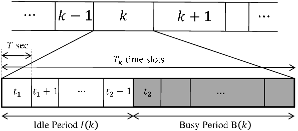
Frame $k$ consists of $T_{k}\triangleq|{\mathcal{F}}(k)|$ consecutive time-slots, where ${\mathcal{F}}(k)$ is the set containing the indices of the time slots belonging to frame $k$ (see Fig. 2). Each frame consists of exactly one idle period followed by exactly one busy period, both are defined next.

The duration of the idle period $I(k)$ and busy period $B(k)$ of frame $k$ are random variables, thus $T_{k}=I(k)+B(k)$ is random as well. Since frames do not overlap, if $t\in{\mathcal{F}}(k_{1})$ then $t\notin{\mathcal{F}}(k_{2})$ as long as $k_{1}\neq k_{2}$. We can write an equation for the average delay as

where ${\mathcal{A}}_{i}(k)\triangleq\cup_{t\in{\mathcal{F}}(k)}{\mathcal{A}}_{i}^{(t)}$ is the set of all packets that arrive at ${\rm SU}_{i}$’s buffer during frame $k$. We note that the long-term average delay $\overline{W}_{i}$ in (5) depends on the chosen priority lists as well as the power allocation policy, in all frames $k\geq 0$.

We are interested to find the optimum scheduling-and-power-allocation policy that minimizes the sum of SUs’ average delays subject to per-SU delay constraint as well as some interference constraints. In this paper, we consider two kinds of interference constraints: 1) instantaneous interference constraint; 2) average interference constraint. Since time-slot-based policies that update the scheduling and power-allocation each time-slot suffer from curse of dimensionality [5], we restrict our problem to frame-based scheduling policies as well as frame-based power allocation policies. The former is represented by the priority list ${\bm{\pi}}(k)$ discussed earlier. On the other hand, the latter is defined in the following definition.

Consider the following constraints

where $I$ denotes the long-term average interference received by the PU while $\mathds{1}(x)\triangleq 1$ if $x\neq 0$ and $0$ otherwise. Constraint (7) is the average delay constraint for ${\rm SU}_{i}$, (8) is the maximum power constraint due to the limitations of ${\rm SU}_{i}$’s transmitter as well as the minimum power constraint that results in finite delays for all SUs ($P_{\rm min}$ is some constant that will be defined later), (9) is the instantaneous interference constraint for the PU, (10) indicates that no more than a single SU is to be transmitting at slot $t$, while the last constraint (11) is to protect the PU from average interference. The two optimization problems that we solve in this paper are

and

We refer to problem (12) as the instantaneous interference constraint problem, while to (13) as the average interference constraint problem. In the next section we solve these two problems and show that their solutions are different.

In order to guarantee a feasible solution satisfying the delay constraints in problems (12) and (13), we set up a “virtual queue” associated with each delay constraint $\overline{W}_{i}\leq d_{i}$. The virtual queue will be used in both problems (12) and (13). The virtual queue for ${\rm SU}_{i}$ at frame $k$ is given by

where $r_{i}(k)\in[0,d_{i}]$ is an auxiliary random variable, that is to be optimized over and $Y_{i}(0)\triangleq 0$, $\forall i$. We define ${\bf Y}(k)\triangleq[Y_{1}(k),\cdots,Y_{N}(k)]^{T}$. Equation (14) is calculated at the end of frame $k-1$ and represents the amount of delay exceeding the delay bound $d_{i}$ for ${\rm SU}_{i}$ up to the beginning of frame $k$. We use the definition of mean rate stability as in [5] to state the following lemma.

Lemma 1 provides a condition on the virtual queue $\{Y_{i}(k)\}_{k=0}^{\infty}$ so that ${\rm SU}_{i}$’s average delay constraint $\overline{W}_{i}\leq d_{i}$ in (7) is satisfied. That is, if the proposed joint power allocation and scheduling policy results in a mean rate stable $\{Y_{i}(k)\}_{k=0}^{\infty}$, then $\overline{W}_{i}\leq d_{i}$. For both problems, the proposed policy depends on the Lyapunov optimization where the goal is to choose the joint scheduling and power allocation policy that minimizes the drift-plus-penalty. In Section IV-B (Section IV-C) we will show that if problem (12) (problem (13)) is feasible, then the proposed policy guarantees mean rate stability for the queues $\{Y_{i}(k)\}_{k=0}^{\infty}$.

We now propose the Delay Optimal with Instantaneous Interference Constraint (DOIC) policy that solves problem (12). This policy is executed at the beginning of each frame $k$ for finding ${\bf P}^{(t)}$ as well as the optimum list ${\bm{\pi}}(k)$, given some prespecified control parameter $V$. Define the random variable $R_{i}(P)$ as (not to be confused with $R_{i}^{(t)}$ in (1))

where $P$ is some fixed constant argument and define $\mu_{i}(P)\triangleq\E\left[R_{i}(P)\right]/L$ where the expectation is taken over $g_{i}^{(t)}$ and $\gamma_{i}^{(t)}$. We now present the DOIC policy, its optimality and then the intuition behind it.
DOIC Policy (executed at the beginning of frame $k$):

1. 1.

   The BS sorts the SUs according to the descending order of $Y_{i}(k)\mu_{i}(P_{\rm max})$. The sorted list is denoted by ${\bm{\pi}}(k)$.

2. 2.

   At the beginning of each slot $t\in{\mathcal{F}}(k)$ the BS schedules ${\rm SU}_{i^{*}}$ that has the highest priority in the list ${\bm{\pi}}(k)$ among those having non-empty buffers.

3. 3.

   ${\rm SU}_{i^{*}}$, in turn, transmits $M_{i^{*}}^{(t)}$ packets as dictated by (2) where $P_{i}^{(t)}=0$ $\forall i\neq i^{*}$ while $P_{i^{*}}^{(t)}$ is calculated as

   $$P_{i^{*}}^{(t)}=\min\left(\frac{I_{\rm inst}}{g_{i^{*}}^{(t)}},P_{\rm max}\right),$$

   (17)

4. 4.

   At the end of frame $k$, for all $i\in{\mathcal{N}}$ the BS updates:

   1. (a)

      $r_{i}(k)=d_{i}$ if $V<Y_{i}(k)\lambda_{i}$, and $r_{i}(k)=0$ otherwise, and then

   2. (b)

      $Y_{i}(k+1)$ via (14).

Before we discuss the optimality of the DOIC in Theorem 1, we define the following quantities. Let $a\triangleq 1-\Pi_{i=1}^{N}\left(1-\lambda_{i}\right)$ denote the probability of receiving a packet from a user or more at a given time slot, while $C_{Y}\triangleq\sum_{i=1}^{N}C_{Y_{i}}$ with $C_{Y_{i}}\triangleq\sqrt{\E\left[A^{4}\right]\E\left[B^{4}\right]}+d_{i}^{2}\E\left[A^{2}\right]$, where $\E\left[A^{2}\right]$ and $\E\left[A^{4}\right]$ are bounds on the second and fourth moments of the total number of arrivals $\sum_{i}|{\mathcal{A}}_{i}(k)|$ during frame $k$, respectively, while $\E\left[B^{4}\right]$ is a bound on the fourth moment of the busy period $B(k)$. The finiteness of these moments can be shown to hold if the first four moments of the service time are finite. In Appendix B we show that all the service time moments exist given any distribution for $P_{i}^{(t)}\gamma_{i}^{(t)}$. We omit the derivation of these bounds due to lack of space.

Theorem 1 says that the objective function of problem (12) is upper bounded by the optimum value $\sum_{i}\overline{W}_{i}^{*}$ plus some constant gap that vanishes as $V\rightarrow\infty$. Having a vanishing gap means that the DOIC policy is asymptotically optimal. Moreover, based on the mean rate stability of the queues $\{Y_{i}(k)\}_{k=0}^{\infty}$, the set of delay constraints of problem (12) is satisfied.

The intuition behind the DOIC policy comes from the proof of Theorem 1. In the proof, we follow the Lyapunov optimization technique to obtain an expression for the drift-plus-penalty then upper bound this expression (see (31)). The DOIC policy becomes the one that minimizes this upper bound or, simply, minimizing $\Phi$ which is given by

Minimizing the first summation in $\Phi_{\rm I}$ minimizes objective function in (12), while minimizing the second summation guarantees that the solution is feasible. We observe that the first term in (19) can be minimized independent of the second term. Step 4.a in the DOIC policy minimizes the first term in (19) while, using the $c\mu$ rule [27], the second term is minimized in Step 1.

In the DOIC policy, the drawback of setting $V$ very large is that the time needed for the algorithm to converge increases. This increase is linear in $V$ [28]. That is, if the number of frames required for the quantity $\sum_{i}{Y_{i}(k)}/(Nk)$ to be less than $\epsilon$ (for some $\epsilon>0$) is $O(K_{1})$, then increasing $V$ to $\beta V$ will require $O(\beta K_{1})$ frames for it to be less than $\epsilon$, for any $\beta>1$. We note that the complexity of the DOIC policy is $O(N)$ because calculating $\mu_{i}(P_{\rm max})$ is of $O(1)$, while the power is closed-form in (17). We note that if problem (12) is not feasible, then this is because one of two reasons; either one or more of the constraints is stringent, or otherwise because $\sum_{i=1}^{N}\lambda_{i}/\mu_{i}(P_{\rm max})\geq 1$. If it is the former, then the DOIC policy will result in a point that is as close as possible to the feasible region. On the other hand, if it is the latter, then we could add an admission controller that limits the average number of packets arriving at buffer $i$ to $\lambda_{i}(1-\epsilon)/\left(\sum_{i=1}^{N}\lambda_{i}/\mu_{i}(P_{\rm max})\right)$ for some $\epsilon>0$.

We now propose the Delay-Optimal-with-Average-Interference-Constraint DOAC policy for problem (13). We first give the following useful definitions. Since the scheduling scheme in frame $k$ is a priority scheduling scheme with preemptive-resume queuing discipline, then given the priority list ${\bm{\pi}}$ we can write the expected waiting time of all SUs in terms of the average residual time [25, pp. 206] defined as $T_{\pi_{j}}^{\rm R}\triangleq\sum_{l=1}^{j}\lambda_{\pi_{l}}\E\left[s_{\pi_{l}}^{2}\right]/2$, where the expectation is taken over $P_{\pi_{l}}^{(t)}\gamma_{\pi_{l}}^{(t)}$. The waiting time of SU $\pi_{j}$ that is given the $j$th priority is [25, pp. 206]

where $\rho_{i}(P)\triangleq\lambda_{i}/\mu_{i}(P)$ and $\overline{\rho}_{\pi_{j-1}}\triangleq\sum_{l=1}^{j-1}\rho_{\pi_{l}}(P_{\pi_{l}})$. Moreover, we define

where $\overline{\rho}^{\rm max}_{i}$ is some upper bound on $\overline{\rho}_{i}$ that will be defined later. We henceforth drop all the arguments of $W^{\rm up}_{\pi_{j}}(P,\overline{\rho}^{\rm max}_{\pi_{j-1}})$ except $P$ and $\overline{\rho}^{\rm max}_{\pi_{j-1}}$ and all those of $W_{\pi_{j}}(P)$ except $P$.

To track the average interference at the PU up to the end of frame $k$ we set up the following virtual queue that is associated with the average interference constraint in problem (13) and is calculated at the BS at the end of frame $k$.

where the term $\sum_{i=1}^{N}{\sum_{t\in{\mathcal{F}}(k)}{P_{i}^{(t)}g_{i}^{(t)}}}$ represents the aggregate amount of interference energy received by the PU due to the transmission of the SUs during frame $k$. Hence, this virtual queue is a measure of how much the SUs have exceeded the interference constraint above the level $I_{\rm avg}$ that the PU can tolerate. Lemma 2 provides a sufficient condition for the interference constraint of problem (13) to be satisfied.

Lemma 2 says that if the power allocation and scheduling algorithm results in mean rate stable $\{X(k)\}_{k=0}^{\infty}$, then the interference constraint of problem (13) is satisfied.

Before presenting the DOAC policy, we first discuss the idea behind it. Intuitively, a policy that solves problem (13) should allocate ${\rm SU}_{i}$’s power and assign its priority such that ${\rm SU}_{i}$’s expected delay and the expected interference to the PU is minimized. The DOAC policy is defined as the policy that selects the power parameter vector ${\bf P}(k)\triangleq[P_{1}(k),\cdots,P_{N}(k)]^{T}$ jointly with the priority list ${\bm{\pi}}(k)$ that minimizes $\Psi\triangleq\sum_{j=1}^{N}\psi_{\pi_{j}}(P_{\pi_{j}}(k),\overline{\rho}^{\rm max}_{\pi_{j-1}})$ where

with $\psi^{\rm D}_{\pi_{j}}(P,\overline{\rho}^{\rm max}_{\pi_{j-1}})\triangleq Y_{\pi_{j}}(k)\lambda_{\pi_{j}}W^{\rm up}_{\pi_{j}}(P,\overline{\rho}^{\rm max}_{\pi_{j-1}})$ while $\psi^{\rm I}_{\pi_{j}}(P)\triangleq X(k)\rho_{\pi_{j}}(P)P\bar{g}_{\pi_{j}}$. The function $\psi^{\rm D}_{\pi_{j}}(P,\overline{\rho}^{\rm max}_{\pi_{j-1}})$ (and $\psi^{\rm I}_{\pi_{j}}(P)$) represents the amount of delay (interference) that SU $\pi_{j}$ is expected to experience (to cause to the PU) during frame $k$.

The brute search of ${\bf P}{}(k)$ and ${\bm{\pi}}(k)$ that minimizes $\Psi$ is exponentially high. To minimize $\Psi$ in a computationally efficient way, we need the functions $\psi_{\pi_{j}}(P_{\pi_{j}}(k),\overline{\rho}^{\rm max}_{\pi_{j-1}})$ to become decoupled for all $j\in{\mathcal{N}}$. That is, we want $\psi_{\pi_{j}}(P_{\pi_{j}}(k),\overline{\rho}^{\rm max}_{\pi_{j-1}})$ not to depend on $P_{\pi_{l}}(k)$ as long as $l\neq j$. Hence, we set the function $\overline{\rho}^{\rm max}_{\pi_{j-1}}$ to some function that does not depend on the optimization power variables $P_{\pi_{l}}(k)$ for all $l\leq j-1$ but otherwise on some other fixed parameters. We need to choose these parameters such that the bound

is satisfied. Thus, these functions, are given by

where

With $\overline{\rho}^{\rm max}_{\pi_{j-1}}$ given by (25), $\psi_{\pi_{j}}(P_{\pi_{j}}(k),\overline{\rho}^{\rm max}_{\pi_{j-1}})$ is a function in $P_{\pi_{j}}(k)$ only. Before we show that the choice of (25) and (26) guarantees that (24) is satisfied, we note that (25) dictates that in order to find $\overline{\rho}^{\rm max}_{\pi_{j-1}}$ we need to find $P_{\pi_{l}}^{\overline{\rho}^{\rm max}}$ for all $l<j-1$. Hence, we find $P_{\pi_{j}}^{\overline{\rho}^{\rm max}}$ recursively starting from $j=1$ at which $\overline{\rho}^{\rm max}_{\pi_{0}}=0$ by definition. It is shown in [29, Lemma 5, pp. 55] that $\overline{\rho}^{\rm max}_{\pi_{j}}$ is an upper bound on $\overline{\rho}_{\pi_{j}}$. $\overline{\rho}^{\rm max}_{\pi_{j}}$ has an advantage over $\overline{\rho}_{\pi_{j}}$ (and hence $\psi_{\pi_{j}}\left(P_{\pi_{j}},\overline{\rho}^{\rm max}_{\pi_{j-1}}\right)$ over $\psi_{\pi_{j}}\left(P_{\pi_{j}},\overline{\rho}_{\pi_{j-1}}\right)$) which is that it is not a function in $P_{\pi_{l}}$ for $l\neq j$. This decouples the power search optimization problem to $N$ one-dimensional searches.

After reducing the search complexity of the power vector, we reduce the search complexity of the priority list from $N!$ to $2^{N}$. To do this, we use the dynamic programming illustrated in Algorithm 1 that solves $\min_{{\bm{\pi}}(k),{\bf P}{}(k)}\Psi$. Its search complexity is of $O(MN2^{N})$ where $M$ is the number of iterations in a one-dimensional search, while $O(1)$ is the complexity of calculating $\Psi$ for a given priority list ${\bm{\pi}}(k)$ and a given power vector ${\bf P}{}(k)$. Compared to the complexity of $O(M^{N}\cdot N!)$ which is that of the $N$-dimensional power search along with the brute-force of all $N!$ permutations of priority list ${\bm{\pi}}(k)$, this is a large complexity reduction. However, the $O(MN2^{N})$ is still high if $N$ was large. Finding an optimal algorithm with a lower complexity is extremely difficult since the scheduling and power control problem are coupled. In other words, in order to find the optimum scheduler we need to know the optimum power vector and vice versa. In Section IV-D we propose a sub-optimal policy with a very low complexity and little degradation in the delay performance. We now present the DOAC policy that the BS executes at the beginning of frame $k$.

DOAC Policy (executed at the beginning of frame $k$):

1. 1.

   The BS executes DOAC-Pow-Alloc in Algorithm 1 to find the optimum power parameter vector ${\bf P}^{*}(k)\triangleq[P^{*}_{1}(k),\cdots,P^{*}_{N}(k)]^{T}$ as well as the optimum priority list ${\bm{\pi}}^{*}(k)\triangleq[\pi^{*}_{1}(k),\cdots,\pi^{*}_{N}(k)]^{T}$ that will be used during frame $k$.

2. 2.

   The BS broadcasts the vector ${\bf P}^{*}(k)$ to the SUs.

3. 3.

   At the beginning of each slot $t\in{\mathcal{F}}(k)$, the BS schedules ${\rm SU}_{i^{*(t)}}$ that has the highest priority in the list ${\bm{\pi}}^{*}(k)$ among those having non-empty buffers.

4. 4.

   ${\rm SU}_{i^{*(t)}}$, in turn, transmits $M_{i^{*(t)}}^{(t)}$ bits as dictated by (2) where $P_{i}^{(t)}=0$ for all $i\neq i^{*(t)}$ while $P_{i^{*(t)}}^{(t)}$ is given by (6).

5. 5.

   At the end of frame $k$, for all $i\in{\mathcal{N}}$ the BS updates:

   1. (a)

      $r_{i}(k)=d_{i}$ if $V<Y_{i}(k)\lambda_{i}$, and $r_{i}(k)=0$ otherwise.

   2. (b)

      $X(k+1)$ via (22).

   3. (c)

      $Y_{i}(k+1)$ via (14), $\forall i\in{\mathcal{N}}$.

Define $C_{X}\triangleq\left((1-a)(2+a)+\E\left[B^{2}\right]+2\E\left[B\right](a-a^{2})\right)\times\left(P_{\rm max}^{2}g_{\rm max}^{2}+I_{\rm avg}^{2}\right)/a^{2}$ and $C\triangleq C_{Y}+C_{X}$ where $\E\left[B\right]$ is a bound on the mean of $B(k)$. It can be shown that $\E\left[B\right]$ and $\E\left[B^{2}\right]$ are finite since the first two moments of the service time are finite (see Appendix B). Thus, $C_{X}$ is finite. Next, we state Theorem 2 that discusses the optimality of the DOAC policy.

Similar to Theorem 1, Theorem 2 says that the interference and delay constraints of problem (13) are satisfied since the virtual queues $\{X(k)\}_{k=0}^{\infty}$ and $\{Y_{i}(k)\}_{k=0}^{\infty}$ are mean rate stable. Hence, the performance of the DOAC policy is asymptotically optimal.

The intuition behind the DOAC policy is similar to that behind the DOIC policy with some differences stated here. When upper bounding the drift-plus-penalty term, we obtain the expression $\sum_{i=1}^{N}\left(V-Y_{i}(k)\lambda_{i}\right)r_{i}(k)+\Psi$ where $\Psi$ is defined before (23). Minimizing the first term in this bound is carried out in Step 5.a of the DOAC policy. On the other hand, minimizing $\Psi$ is carried out using the dynamic programming in Algorithm 1. The dynamic programing finds the optimum values of the two vectors ${\bm{\pi}}(k)$ and ${\bf P}(k)$ in an efficient way of complexity $O(NM2^{N})$ without having to calculate the objective function $\Psi$ for the whole sample space of size $N!\times M^{N}$. The reason we were able to use this algorithm is because we were able to find an upper bound $W^{\rm up}_{\pi_{j}}$ that does not depend on the vector ${\bm{\pi}}(k)$, a property that is necessary for the dynamic programming and that is absent in $\overline{W}_{\pi_{j}}$.

As seen in the DOAC policy, the complexity of finding the optimal power vector and priority list can be high when the number of SUs $N$ is large. This is mainly due to the large complexity of Algorithm 1. In this subsection we propose a suboptimal solution with an extreme reduction in complexity and with little degradation in the performance. This solution solves for the power allocation and scheduling algorithm, thus it replaces the Algorithm 1.

The challenges in Algorithm 1 are three-fold. First finding the priority list (scheduling problem) requires the search over $N!$ possibilities. Second, even with a genie-aided knowledge of the optimum list, we still have to carry-out $N$ one-dimensional searches to find ${\bf P}^{*}(k)$ (power control problem). Third, the scheduling and power control problems are coupled. We tackle the latter two challenges first, by finding a low-complexity power allocation policy that is independent of the scheduling algorithm. Then we use the $c\mu$ rule [27] to find the priority list. The $c\mu$ rule is a policy that gives the priority list that minimizes the quantity $\sum_{i=1}^{N}Y_{i}(k)\lambda_{i}W_{i}(P_{i}(k))$, given some power allocation vector ${\bf P}(k)$.

References

- [1] A. E. Ewaisha and C. Tepedelenlioğlu, “Dynamic scheduling for delay guarantees for heterogeneous cognitive radio users,” in 2015 49th Asilomar Conference on Signals, Systems and Computers, Nov 2015, pp. 169–173.
- [2] Sanjay Shakkottai and Rayadurgam Srikant, “Scheduling real-time traffic with deadlines over a wireless channel,” Wireless Networks, vol. 8, no. 1, pp. 13–26, 2002.
- [3] X. Kang, W. Wang, J.J. Jaramillo, and L. Ying, “On the performance of largest-deficit-first for scheduling real-time traffic in wireless networks,” in Proceedings of the fourteenth ACM international symposium on Mobile ad hoc networking and computing. ACM, 2013, pp. 99–108.
- [4] Arash Asadi and Vincenzo Mancuso, “A survey on opportunistic scheduling in wireless communications,” Communications Surveys & Tutorials, IEEE, vol. 15, no. 4, pp. 1671–1688, 2013.
- [5] C.-P. Li and M.J. Neely, “Delay and Power-Optimal Control in Multi-Class Queueing Systems,” ArXiv e-prints, Jan. 2011.
- [6] Michael J Neely, Eytan Modiano, and Charles E Rohrs, “Power allocation and routing in multibeam satellites with time-varying channels,” IEEE/ACM Transactions on Networking, vol. 11, no. 1, pp. 138–152, 2003.
- [7] Hussein Al-Zubaidy, Ioannis Lambadaris, and Jerome Talim, “Optimal scheduling in high-speed downlink packet access networks,” ACM Trans. Model. Comput. Simul., vol. 21, no. 1, pp. 3:1–3:27, Dec. 2010.
- [8] K. Jagannathan, M.G. Markakis, E. Modiano, and J.N. Tsitsiklis, “Throughput optimal scheduling over time-varying channels in the presence of heavy-tailed traffic,” Information Theory, IEEE Transactions on, vol. 60, no. 5, pp. 2896–2909, May 2014.
- [9] K. Hamdi, Wei Zhang, and K.B. Letaief, “Uplink scheduling with qos provisioning for cognitive radio systems,” in Wireless Communications and Networking Conference, 2007.WCNC 2007. IEEE, march 2007, pp. 2592 –2596.
- [10] Yonghong Zhang and C. Leung, “Resource allocation in an OFDM-based cognitive radio system,” IEEE Transactions on Communications, vol. 57, no. 7, pp. 1928–1931, July 2009.
- [11] R. Urgaonkar and M.J. Neely, “Opportunistic scheduling with reliability guarantees in cognitive radio networks,” Mobile Computing, IEEE Transactions on, vol. 8, no. 6, pp. 766–777, 2009.
- [12] Shaowei Wang, Zhi-Hua Zhou, Mengyao Ge, and Chonggang Wang, “Resource allocation for heterogeneous cognitive radio networks with imperfect spectrum sensing,” IEEE Journal on Selected Areas in Communications, vol. 31, no. 3, pp. 464–475, March 2013.
- [13] C. Yi and J. Cai, “Two-stage spectrum sharing with combinatorial auction and stackelberg game in recall-based cognitive radio networks,” IEEE Transactions on Communications, vol. 62, no. 11, pp. 3740–3752, Nov 2014.
- [14] C. Yi and J. Cai, “Multi-item spectrum auction for recall-based cognitive radio networks with multiple heterogeneous secondary users,” IEEE Transactions on Vehicular Technology, vol. 64, no. 2, pp. 781–792, Feb 2015.
- [15] Z. Guan, T. Melodia, and G. Scutari, “To transmit or not to transmit? distributed queueing games in infrastructureless wireless networks,” Networking, IEEE/ACM Transactions on, vol. PP, no. 99, pp. 1–14, 2015.
- [16] A.E. Ewaisha and C. Tepedelenlioğlu, “Throughput optimization in multichannel cognitive radios with hard-deadline constraints,” IEEE Transactions on Vehicular Technology, vol. 65, no. 4, pp. 2355–2368, April 2016.
- [17] A. E. Ewaisha and C. Tepedelenlioğlu, “Throughput Maximization in Multichannel Cognitive radio Systems with Delay Constraints,” in the 47th Asilomar Conference on Signals, Systems, and Computers, 2013. IEEE, November 2013.
- [18] Zhenwei Li, Changchuan Yin, and Guangxin Yue, “Delay-bounded power-efficient packet scheduling for uplink systems of lte,” in Wireless Communications, Networking and Mobile Computing, 2009. WiCom ’09. 5th International Conference on, Sept 2009, pp. 1–4.
- [19] Mohammad M Rashid, Md J Hossain, Ekram Hossain, and Vijay K Bhargava, “Opportunistic spectrum scheduling for multiuser cognitive radio: a queueing analysis,” Wireless Communications, IEEE Transactions on, vol. 8, no. 10, pp. 5259–5269, 2009.
- [20] Jian Wang, Aiping Huang, Lin Cai, and Wei Wang, “On the queue dynamics of multiuser multichannel cognitive radio networks,” Vehicular Technology, IEEE Transactions on, vol. 62, no. 3, pp. 1314–1328, March 2013.
- [21] A. S. Zahmati, X. Fernando, and A. Grami, “Energy-aware secondary user selection in cognitive sensor networks,” IET Wireless Sensor Systems, vol. 4, no. 2, pp. 86–96, June 2014.
- [22] Simon Haykin, “Cognitive radio: brain-empowered wireless communications,” Selected Areas in Communications, IEEE Journal on, vol. 23, no. 2, pp. 201–220, 2005.
- [23] M. Bari and M. Doroslovački, “Order recognition of continuous-phase FSK,” in Proc. 49th Asilomar Conference on Signals, Systems, and Computers, Pacific Grove, CA, USA, Nov. 8-11 2015, pp. 913–917.
- [24] M. Bari, A. Khawar, M. Doroslovački, and T. Clancy, “Recognizing FM, BPSK and 16-QAM using supervised and unsupervised learning techniques,” in Proc. 49th Asilomar Conference on Signals, Systems, and Computers, Pacific Grove, CA, USA, Nov. 8-11 2015.
- [25] D.i Bertsekas and R. Gallager, Data Networks (2Nd Ed.), Prentice-Hall, Inc., Upper Saddle River, NJ, USA, 1992.
- [26] Freescale Semiconductor, “Long term evolution protocol overview,” White Paper, Document No. LTEPTCLOVWWP, Rev 0 Oct, 2008.
- [27] David D Yao, “Dynamic scheduling via polymatroid optimization,” in Performance Evaluation of Complex Systems: Techniques and Tools, pp. 89–113. Springer, 2002.
- [28] Michael J Neely, Dynamic power allocation and routing for satellite and wireless networks with time varying channels, Ph.D. thesis, Citeseer, 2003.
- [29] Ahmed Ewaisha, “Scheduling and power allocation to optimize service and queue-waiting times in cognitive radio uplinks,” CoRR, vol. abs/1601.00608, 2016.
- [30] CISCO, “Implementing quality of service over cisco mpls vpns,” 2006.
- [31] L. Georgiadis, M.J. Neely, and L. Tassiulas, Resource allocation and cross-layer control in wireless networks, Now Publishers Inc, 2006.
- [32] R. Urgaonkar, B. Urgaonkar, M.J. Neely, and A. Sivasubramaniam, “Optimal power cost management using stored energy in data centers,” in Proceedings of the ACM SIGMETRICS Joint International Conference on Measurement and Modeling of Computer Systems, New York, NY, USA, 2011, pp. 221–232, ACM.
- [33] M.H. DeGroot and M.J. Schervish, Probability and Statistics, Pearson Education, fourth edition, 2011.
- [34] Adithya Rajan, On the Ordering of Communication Channels, Ph.D. thesis, Arizona State University, 2014.
![[Uncaptioned image]](1602.08010v3/authorAhmed_Ewaisha.png) |
Ahmed E. Ewaisha was born in Cairo, Egypt in 1987. He received his B.S. degree with honors in electrical engineering ranking top 5% on his class at Alexandria University in 2009. Consequently, he was admitted to Nile University that is considered the first research-based university in Egypt where he received his M.S. degree in 2011 in wireless communications. In fall 2011, he joined the Ira A. Fulton School of engineering at Arizona State University, Tempe, where he is now working towards his PhD degree studying the delay analysis in cognitive radio networks. His research interests span a wide area of wireless as well as wired communication networks including stochastic optimization, power allocation, cognitive radio networks, resource allocation and quality-of-service guarantees in data networks. |
![[Uncaptioned image]](1602.08010v3/authorCihan_Tepedelenlioglu.png) |
Cihan Tepedelenlioğlu (S’97-M’01) was born in Ankara, Turkey in 1973. He received his B.S. degree with highest honors from Florida Institute of Technology in 1995, and his M.S. degree from the University of Virginia in 1998, both in electrical engineering. From January 1999 to May 2001 he was a research assistant at the University of Minnesota, where he completed his Ph.D. degree in electrical and computer engineering. He is currently an Associate Professor of Electrical Engineering at Arizona State University. Prof. Tepedelenlioğlu was awarded the NSF (early) Career grant in 2001, and has served as an Associate Editor for several IEEE Transactions including IEEE Transactions on Communications, IEEE Signal Processing Letters, and IEEE Transactions on Vehicular Technology. His research interests include statistical signal processing, system identification, wireless communications, estimation and equalization algorithms for wireless systems, multi-antenna communications, OFDM, ultra-wideband systems, distributed detection and estimation, and data mining for PV systems. |