Contrasting Effects of Replication in Parallel Systems: From Overload to Underload and Back
Abstract
Task replication has recently been advocated as a practical solution to reduce latencies in parallel systems. In addition to several convincing empirical studies, some others provide analytical results, yet under some strong assumptions such as Poisson arrivals, exponential service times, or independent service times of the replicas themselves, which may lend themselves to some contrasting and perhaps contriving behavior. For instance, under the second assumption, an overloaded system can be stabilized by a replication factor, but can be sent back in overload through further replication. In turn, under the third assumption, strictly larger stability regions of replication systems do not necessarily imply smaller delays.
Motivated by the need to dispense with such common and restricting assumptions, which may additionally cause unexpected behavior, we develop a unified and general theoretical framework to compute tight bounds on the distribution of response times in general replication systems. These results immediately lend themselves to the optimal number of replicas minimizing response time quantiles, depending on the parameters of the system (e.g., the degree of correlation amongst replicas). As a concrete application of our framework, we design a novel replication policy which can improve the stability region of classical fork-join queueing systems by , in the number of servers .
I Introduction
Despite a significant increase in network bandwidth and computing resources, major online service providers (and not only) still face extremely volatile revenues due to the high variability of latencies (aka response times/delays), especially in their tails (e.g., the -percentile). Several well-cited and convincing studies reported significant potential revenue loss by Google, Bing, or Amazon, were the latencies higher [25, 13, 27]; a typical cited argument is that an additional ms in latency would cost Amazon of sales.
Given the late abundance of computing resources, a natural and yet very simple way to improve latencies is replication, a concept which was traditionally used to improve the reliability of fault-tolerant systems [24]. In the context of a multi-server (parallel) system, the idea is merely to replicate a task into multiple copies/replicas, and to execute each replica on a different server. By leveraging the statistical variability of the servers themselves, as execution platforms, it is expected that some replicas would finish much faster than others; for a discussion of various system/OS factors affecting execution times see [5]. The key gain of executing multiple replicas is not to reduce the average latency, but rather the latency tail which is recognized as critically important for ensuring a consistently fluid/natural responsiveness of systems. Therefore, replication can be regarded as being instrumental to the development of “latency tail-tolerant systems”, similarly to its role in fault-tolerant systems [5].
While the idea of using redundant requests is not new, as it has been used to demonstrate significant speedups in parallel programs [10, 12], it has become very attractive with its implementation in the MapReduce framework through the so-called ‘backup-tasks’ [6]. Thereafter there has been a surge of very high-quality empirical work which has convincingly demonstrated the benefits of using redundancy for significant latency improvement, both in the mean and also top percentiles. Such works include latency reductions in Google’s distributed systems [4], in DNS queries and database servers [29], key-value storage systems [28], cloud storage systems [33], or significant speed-ups of small jobs in data-centers [1] or short TCP flows [34].
Such empirical work has been complemented by several excellent analytical studies (see the Related Work section), which have provided fundamental insight into the benefits of replication. Constrained by analytical tractability, most of these works make several strong assumptions: not only the arrivals are Poisson and the service times are exponentially distributed (i.e., typical assumptions in the queueing literature), but the service times of the replicas plus the corresponding original tasks are statistically independent. By challenging these assumptions, especially the last two, we first provide some elementary analytical arguments, along with some simulation results, that the benefits of replication are highly dependent on both the distributional and correlation structures of the service times. A convincing example is that the stability region of a system is not monotonous in the replication factor. For instance, by adding a replica server an overloaded system can be stabilized, an advantage which however vanishes by adding additional replica servers, whence the subtitle of this paper.
The contribution of this paper is a general analytical framework to compute stochastic bounds on the response time distributions in replication systems. In particular, our framework covers scenarios with Markovian arrivals, general service time distributions (subject to a finite moment generating function), and a correlation model amongst the original and replicated tasks. Using back-of-the-envelope calculations, our results can be immediately used for engineering purposes (e.g., to determine the optimum number of replicated servers to minimize the top percentiles of latencies). A key feature of our methodology is that it relies on a powerful martingale methodology which was recently shown to provide remarkably accurate stochastic bounds in various and challenging queueing systems with non-Poisson arrivals (see, e.g., [3, 21, 23]). According to several numerical/simulation illustrations, our results exhibit a similar high accuracy, including the challenging case of Markovian arrivals.
To concretely illustrate the applicability of our results we consider two applications. The first is to improve the performance of MapReduce systems (which can be abstracted by a Fork-Join (FJ) queueing model) through replication. In particular, we design an elementary replication policy which can significantly improve not only delay quantiles (e.g., by a factor of roughly ), but more fundamentally the stability region of a FJ system by a logarithmic factor in the number of servers ; our analysis provides a theoretical understanding of the benefits of using back-up tasks in MapReduce, as a proposal to alleviate the problem of stragglers [6]. Albeit such a theoretical benefit is obtained under strong exponential and statistical independence assumptions, simulation results show that the underlying numerical benefits carry over to realistic scenarios subject to correlations amongst replicas. The second application investigates the analytical tradeoff between resource usage and response times under replication, a matter which has recently been addressed through Google and Bing empirical studies. The key analytical insight is that increasing resource usage through replication yields a substantial reduction of response time upper quantiles if the service times of the replicas are sufficiently independent (i.e., subject to a low correlation factor, to be later formally described).
The rest of the paper is organized as follows. In Section § II we introduce the analytical models and discuss related work. In Section § III we provide several insights into the benefits of replication, by following elementary models and derivations. In Section § IV we provide our general theoretical framework dealing with both Poisson and Markovian arrivals, and also independent and correlated replicas (i.e., four scenarios). In Section § V we investigate the two applications of our analytical framework. In Section § VI we conclude the paper.
II Replication Models and Related Work
We consider a parallel system with homogeneous servers with identical speeds (see Figure 1). A stream of tasks arrives at a dispatcher according to some stationary and ergodic point process; the interarrival times are denoted by with the mean , whereas their number within the (continuous) time interval is denoted by . This process can have a Markov structure, to be more precisely defined in Section § IV-B.
The service times of the tasks are denoted by and are drawn from some general distribution subject to a finite moment generating function; the average is set to . For numerical purposes, we will occasionally use the analytically convenient Pareto distribution, which can be approximated within our theoretical framework through a hyperexponential distribution.
The utilization of one server, in a system without replicas where tasks are symmetrically distributed, is denoted by
In general, it is assumed for stability that . However, in a system with replication, the expression of the utilization may change depending on various factors (e.g., the distribution of tasks’ service times) whereas the stability condition may fail (such occurrences will be specifically indicated).
II-A Tasks Assignment Policies
A crucial design component in the parallel server system is the task assignment policy, i.e., how are the incoming tasks assigned to the servers for processing? While many such policies have been analytically and empirically studied, we focus on few relevant ones in terms of both performance and overhead:
- •
Random: Each task is dispatched, uniformly at random, to one of the servers; in the particular case of a Poisson (overall) arrival stream, the tasks arrived at some server follow a Poisson distribution with rate .
- •
Round-Robin: Tasks are deterministically dispatched in a circular fashion to the servers, i.e., task is assigned to server (with the convention that stands for ); in the case of a Poisson stream, the interarrival times at some server follow an Erlang distribution.
- •
G/G/K: Unlike the previous two schemes, which immediately dispatch the incoming tasks, and whereby tasks enqueue at the assigned servers, in it is the responsibility of each server to fetch a single task, from a centralized queue at the dispatcher, once they become idle.
- •
(Full-)Replication (-replication factor): Each incoming task is replicated to all the servers11 1 For the sake of clarification, the original task is called a replica as well.; the corresponding service times are denoted by for . Alike in Random and Round-Robin, each server maintains a local (FIFO) queue.
- •
Partial-Replication (-replication factor): Besides full replication, a task may be replicated to only servers; for simplicity, we will assume that both and are powers of , and that consecutive blocks of replicas are allocated to the servers in a round-robin manner. We call the underlying strategy (strict) Partial-Replication when , and No-Replication when .
In terms of analytical tractability, Random and Round-Robin are significantly more amenable than ; in fact, exact results are known for only in the case of Poisson arrivals and exponential service times (in which case the model is denoted by ). However, yields significantly better performance (i.e., much smaller response times of the tasks) than Random and Round-Robin, especially in the case of high variability of the tasks’ service times; in turn Round-Robin slightly outperforms Random (for an excellent related discussion see [11], pp. 408-430).
It is to be noted however that the superiority of is (partly) due to the availability of additional system information, i.e., each task is ‘informed’ about which server is idle such that it can minimize its response time. In turn, amongst policies which are oblivious to such information, Round-Robin was shown to be optimal for exponential [7, 30] and increasing failure rate distributions [20]; for a recent state-of-the-art queueing analysis of Round-Robin see [14].
A more sophisticated replication strategy was proposed in the context of massively parallel data processing systems in which (large) jobs are forked/split into (smaller) tasks, each assigned to a server; once a fraction of the tasks finish their executions, each of the remaining (and straggling) tasks are further replicated. This model appeared in the MapReduce specification [6], and was formally studied in terms of the underlying response time / resource usage tradeoff, albeit by disregarding queueing effects in [31]. Another strategy used by Google is to defer the start of executing the second replica for some suitable time, in order to reduce resource usage [5].
II-B Purging/Cancellation Models
Before discussing the relative performance of Replication to other policies, we first define how replication strategies deal with residual resources.
- •
Purging: A task is considered to complete (and hence its response time is determined) when the fastest replica finishes its execution; at the same time, the residual replicas are all purged/cancelled from the system (with some negligible related cost).
- •
Non-Purging: A task response time is determined as in the Purging case, but the remaining replicas leave the system no sooner than their execution end.
Purging is clearly more efficient from a purely task response-time perspective, as it frees resources once the first replica completes; this operation demands however synchronization overhead amongst the servers. One basic reason for this superiority is that in the Non-Purging model the utilization increases -fold for a -replication factor, for any task service time distribution; in particular, a -replication factor requires the replica-free system to have a utilization under (otherwise the response times get unbounded). In turn, the growth of the utilization is less pronounced in the Purging model, depending on the type of distribution of the service times; in fact, and perhaps counterintuitively, there is no increase in the case of the exponential distribution regardless the replication factor (for a follow-up discussion see § III-B).
Besides the advantage of a better queueing performance, the Purging model is much easier to analyze. In fact, the only analytical study of Non-Purging is considered in [29]; besides the classical and simplifying assumptions of Poisson arrivals and exponential service times, the underlying queueing analysis critically relies on an artificial statistical independence assumption amongst the queues. Using this assumption, it is shown that below a utilization threshold of , a -replication factor strategy does improve the response time despite the inherent doubling of the utilization.
A generalized version of Partial-Replication considers the situation when the fastest replicas finish their execution (the residual ones being subsequently purged); a practical use of this generalization is in coded distributed storage systems [26]. The central result is that under arrivals with independent increments, and exponential (or ‘heavier’) service times, Full-Replication minimizes the (average) response times. In turn, in the case of ‘lighter’ service times and utilization, a replication factor greater than one is detrimental. The underlying proofs use an ingenious coupling argument, but do not provide quantitative results.
Another set of qualitative results, on the superiority of Full-Replication for a specific type of service time distributions (including the exponential) is presented in [19]. Interestingly, under a discrete time model with geometric service time distributions, is is shown in [2] through quantitative results that No-Replication is optimal (for an explanation of the apparent contradiction between exponential and geometric service time distributions, with respect to the optimality of the replication model, see [19]).
Recently, an Early Purging model, in which residual replicas are purged once the first one starts its execution, has been mentioned in [5] and further analyzed in [17]; besides reducing the resource usage, it was shown that this model can also significantly reduce response times despite the apparent loss of diversity, at high utilizations.
The perhaps most fundamental related result obtained so far is a recent exact analysis under the purging model [9]. While the analysis critically relies on the Poisson/exponential models, a key analytical contribution is capturing multi-class arrivals (i.e., different arrival streams are served by different sets of (replicated) servers). The elegance of the results lends itself to several fundamental and contriving insights into the properties of replication, especially accounting for the multi-class feature of the model.
More general stochastic bounds in replication systems are obtained in [8], including the very challenging multi-stage case, by leveraging the analytical power of the stochastic network calculus methodology. While the underlying arrival and service models from [8] are more general than ours, the crucial difference is in handling the underlying correlation structures: concretely, while [8] deals with arbitrary correlation structures yielding stochastic bounds holding in great generality, we exploit the specific correlation structures through the martingale methodology.
III Elementary analytical Insights
Here we complement the previous discussion by providing several motivating examples. After quickly contrasting the task assignment policies introduced earlier, under the Poisson/exponential models, we explore more general service time distributions. The key insight is that the stability region of replicated systems is not necessarily monotonous in the number of replicas; depending on the service distribution, any of the policies No-Replication, Full-Replication, or Partial-Replication can yield the largest stability region.
III-A The M/M model
For some immediate analytical insight, consider the classical example of Poisson arrivals and exponential service times. Due to a lack of closed-form formulas for all considered policies, for large number of servers, we assume that ; recall that the (server) utilization is .
The average response times for the four policies (i.e., Random, Round-Robin, M/M/2, and Replication) are, respectively,
Note that Replication induces an queueing model, in which the service time is the first order statistics of two i.i.d. random variables (in the current case being an exponential with half of the mean of the original). Immediate comparisons reveal that the minimum (‘best’) response time is attained by Replication; a key reason is that the gain of sampling the minimum of exponential random variables, together with the Purging model, significantly dominates the cost of temporary redundant resource usage. In turn, the maximum (‘worst’) response time is attained by Random; the relative performance of Round-Robin and M/M/2 depends on the value of . Lastly, we point out that the superiority of Replication immediately extends to larger values of .
More general results in terms of lower and upper bounds on the average response time in the case of a variant of Replication, in which only the fastest tasks are required to complete (whilst the residual tasks are purged) (and which was qualitatively studied in [26]), appeared in [16]; in particular, it was shown that Replication outperforms the corresponding M/M/K model. Further upper bounds were derived in the case of general service time distributions, using existing bounds on the first two moments of the order statistics.
III-B Beyond the M model
In the previous example with exponential service times, the stability region is invariant to the replication factor; the reason is that the order statistic of (independent) exponential random variables is an exponential random variable . The next elementary examples show that any strategy amongst No-Replication, Full-Replication, or Partial-Replication can yield the strictly largest stability regions (and hence ‘best’ response times, at least in some subset of the stability region; a follow-up discussion will be given in Section § IV-C). A fundamental reason is the assumption of independent service times of the replicas, which motivates the need for accounting for some correlation structures.
Recall that in the No-Replication scenario, a necessary and sufficient condition for stability (or, equivalently, for finite response times) is
In the case of Full-Replication, the corresponding stability condition is given by
whereas in the case of Partial-Replication with replication factor by
| (1) |
Denoting the CCDF of by
we observe from the previous stability conditions that the ‘best’ replication-factor is
| (2) |
We next present examples of different distributions for resulting in ‘best’ scenarios for each of the three replication strategies.
III-B1 No-Replication: Uniform
Assume uniformly distributed service times, i.e., . The following argument shows that in this case replication is detrimental, i.e.,
for any :
The same argument additionally shows that Partial-Replication is better than Full-Replication. This result extends the qualitative observation from [26] (i.e., Theorem 4 therein, restricted to a utilization, and hence an unstable regime) to any (stable) utilization.
III-B2 Full-Replication: Weibull
Let the now be Weibull distributed, i.e., . For , a higher degree of replication is ‘better’, as shown below:
By the assumption on , the last term is monotonically decreasing in . Note that in the special case of exponentially distributed , i.e., , replication is neither beneficial nor detrimental (from the point of view of the stability region), as pointed out earlier. This result also extends the qualitative observation from [26] (i.e., Theorem 3) to any (stable) utilization.
III-B3 Partial Replication: Pareto
Lastly we consider the Pareto distribution, i.e., for . For a suitably chosen , it can be shown that (strict) Partial-Replication can become ‘better’ than both Full-Replication and No-Replication:
It is clear that for sufficiently small , the minimal value is attained for .
This last example highlights that the performance of replication strategies heavily depends on the replication factor , the service time distribution, and other underlying assumptions. In particular, performance is not monotonic in , and thus an optimization framework is desirable (related results, on the actual response time distributions as a function of will be provided in the next section).

For complementary numerical results illustrating the counterintuitive effect of , consider the Pareto distribution with the assumption of independent service times of the replicas. Let , arrival rate , (for the Pareto distribution), yielding a utilization (i.e., ). By plotting the simulated latencies of the first packets, Figure 2 shows that while the system without replication is in overload, a replication factor of stabilizes the system (reducing the utilization to ), whereas a replication factor of puts the system back in overload (increasing the utilization to ).
The non-monotonic behavior in disappears when the service times are sufficiently correlated. Indeed, by taking the service times of the replicas as (where the are Pareto distributed, and is arbitrary), it holds:
so that (for a suitably chosen , and a sufficiently large value of ) the optimal value of in Eq. (2) is (i.e., No-Replication is ‘best’).
IV Theory
We assume a queueing system with servers and interarrival times between jobs and denoted by . Upon its arrival, job is replicated to servers where they are processed with service times , respectively. For simplicity, we throughout assume that is an integral multiple of . Further, the jobs are assigned to the batches in a round robin scheme, i.e. the interarrival times for one batch can be described as:
The following recursion describes the response time of job , i.e., the time between the job’s arrival and its service being complete:
resulting in a representation of the steady-state response time as:
| (3) |
where stands for equality in distribution, and the empty sum is by convention equal to .
Depending on the correlation between either the interarrival times and the service times, respectively, we consider four different scenarios: In Subsection § IV-A, all random variables , are assumed to be independent. In Subsection § IV-B, the interarrival times are driven by a certain Markov chain, whereas in Subsection § IV-C the service times are correlated through a common additive factor. Finally, in Subsection § IV-D, a combination of both correlation models is considered.
IV-A Independent Arrivals, Independent Replication
As stated above, we consider the scenario of independent replication, i.e., is an independent family of random variables.
The next Theorem provides an upper bound on the CCDF of as defined in Eq (3):
Theorem 1.
Let be defined by
Then the following bound on the response time holds for all :
Note that, given the stability conditions from Eq. (1), as
Proof.
Define the process by
is a martingale:
Now define the stopping as
and note that . With the optional stopping theorem
Now let . ∎
We point out that the proof essentially follows the bounding technique for GI/GI/1 queues from [18].
IV-B Markovian Arrivals, Independent Replication
We now turn to the more realistic scenario where the interarrival times are correlated: A two-state Markov chain alternates between active and inactive periods; while in the active state, exponentially distributed interarrival times are generated with parameter , and the chain turns inactive with probability . In the inactive state, one interarrival time (exponentially distributed, parameter ) is generated, and the chain jumps back to the active state (see Figure 3). Formally, let
be i.i.d. random variables and define the sequence of interarrival times by
The steady state distribution of the Markov chain is given by
such that for the average of the interarrival times holds
| (4) |
Note that the transition matrix of is given by:
In order to state the main result of this section, we need the following transform of matrix :
Definition 2.
For , let denote the following matrix:
Further, let denote the spectral radius of , and be a corresponding eigenvector.
Note that is an exponential transform of which has the Laplacians of the respective arrival times as an additional factor in each column. In particular, with we recover the transition matrix itself, i.e., .
The following Theorem is the analogous result to Theorem 1 (note that the service times are still assumed to be i.i.d.):
Theorem 3.
Let and be defined by
Then, for the system with replication to out of servers, the following bound on the response time holds for all :
IV-C Independent Arrivals, Correlated Replication
We now address the more realistic scenario when the replicas are no longer independent; we consider the following correlation model (from [16]):
| (5) |
where the random variables and are i.i.d. Here, the parameter describes the degree of correlation amongst the replicas: corresponds to the i.i.d. case from Section § IV-A, whereas for the servers are entirely synchronized so that no replication gain is achieved.
For simplicity the interarrival times are first assumed to be i.i.d. as in Section § IV-A.
Theorem 4.
Let be defined by
Then the following bound on the response time holds for all :
Proof.
Entirely analogous to the proof of Theorem 1. ∎
To illustrate the impact of the correlation parameter we consider the special case when and are exponentially distributed with parameter . Clearly,
so that is the solution of
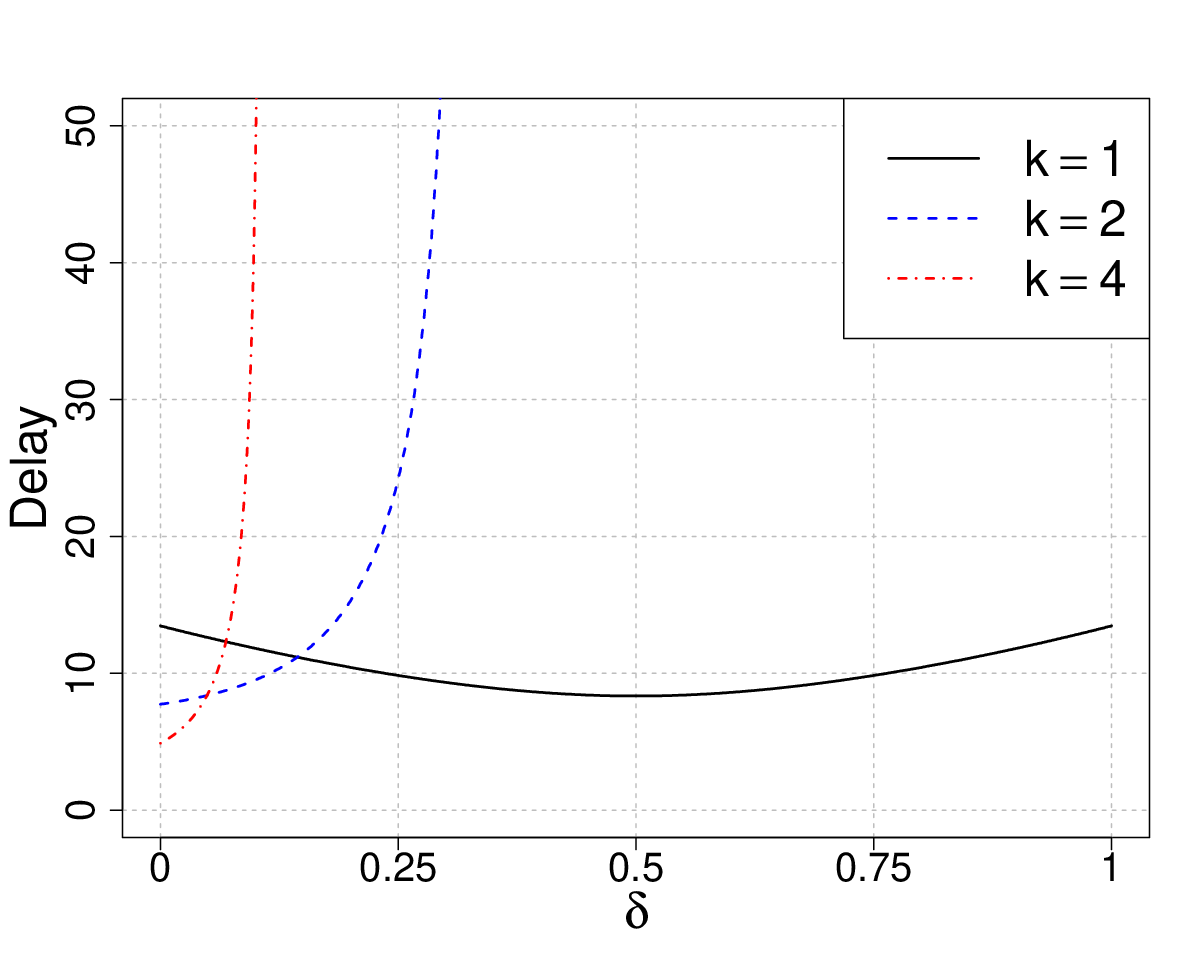
Further, Figure 4 illustrates the -percentile of the delay as a function of the degree of correlation for several numbers of replicas . Strictly from the point of view of the stability region, as it was also considered in Section § III-B, we observe that replication (both and ) is detrimental as the corresponding systems quickly become unstable. In contrast, from the point of view of delays, replication can be beneficial within a subset of the corresponding stability region notwithstanding its strict inclusion in the stability region of the non-replicated system. This fundamental observation can be intuitively explained in that for larger values of the degree of correlation , the servers become more synchronized and consequently no significant replication gain can be achieved; a further follow-up discussion concerning a convergence result depending on will be given in Section § V-A. As a side remark, the symmetry in the delay for is due to the underlying Erlang distribution, which minimizes its variance at .
IV-D Markovian Arrivals, Correlated Replication


Theorem 5.
To numerically compare our stochastic bounds from Theorems 1, 4, 3, and 5 to simulation results we refer to Figures 5(a)-(d), respectively. In all four scenarios, addressing combinations of independent/correlated arrivals and replications, jobs are replicated to out of a total number of servers. The parameters of the respective models are chosen such that the (server) utilization remains constant, i.e., . In particular, in Figure 5a, both the interarrival- and service times are exponentially distributed with parameters and . In Figure 5b, the interarrival times are again exponential with , the correlation factor is , whereas the components and of the service times from Eq. (5) are exponential with parameter
such that . In Figure 5c, the parameters for the Markov chain are , , , whereas the services times are exponential with parameter . According to Eq. (4) the average of the interarrival times is , such that . Finally, in Figure 5d, the parameters for the service times from Figure 5b are combined with the parameters for the interarrival times from Figure 5c. We remark that in all four scenarios the stochastic bounds from Theorems 1, 4, 3, and 5 are remarkably accurate.
V Applications
In this section we present two practical applications of our theoretical framework. The first concerns integrating replication with a fork-join queueing model; a major outcome is the construction of an intuitive class of assignment policies which can fundamentally improve response times. The second investigates the analytical tradeoff between resource usage and response times, an issue which was subject to several measurement studies involving Google and Bing traces.
V-A Fork-Join with Replication (FJR)
In this section we consider replication in the context of a fork-join (FJ) queueing system. In a FJ system, arriving jobs are split into different tasks which are mapped to servers to be processed independently. A job is considered finished once all of its corresponding tasks have finished. We consider the special case of a blocking system whereby jobs cannot be forked before all of the tasks of the previous job have left the system (this mode is in particular characteristic to Hadoop, through a particular coordination service [32]).
The obvious drawback of this blocking model is that it is no longer work-conserving: servers can become idle once some but not all tasks of one job are complete. Moreover, the stability condition of the system becomes a function of the number of servers.
Consider for instance the case of Poisson arrivals with rate and exponential and identically distributed service times , , with rate . As the distribution of the maximum of i.i.d. exponential random variables satisfies [22], the stability condition is roughly
| (6) |
To overcome the issue of decaying stability regions (in the number of servers ) we propose the following task assignment policy which suitably triggers replicas on top of the standard FJ model.
Policy FJR (Fork-Join with Replication): Once a server finishes its task, it immediately replicates a remaining task from another running server. When either the original task or one of its replica has finished, the others are immediately purged.
FJR can be regarded as a concrete implementation of backup-tasks in MapReduce (which is not explicitly presented in the original MapReduce description [6]). Our policy is quite flexible in that the executing task to be replicated can be chosen randomly (yet independently of the current state); moreover, as multiple servers can become idle at the same time (due to the underlying purging model), each can replicate any executing tasks. Intuitively, this flexibility is due to the underlying assumption of exponentially distributed and independent service times.
The main result of the FJR policy is the following:
Theorem 6.
The overall service time of jobs processed by FJR follows an -distribution. Consequently, the corresponding stability condition is
Proof.
Let denote the times where the tasks (original or replica) finish (see Figure 6). Obiviously, it holds . We first show (with the convention ) that the family
is independent and identically exponentially distributed with parameter .
For , this follows directly from the well known fact that the minimum over independent, exponential random variables with rate is exponentially distributed with rate .
Now, suppose tasks finish, or are purged, at time . Denote by the corresponding service times of the respective replicas starting at . For the remaining servers, denote by the service times of the current tasks and by the length of time they started before . Now we can write
Note that the family is independent from one another and from .
Now, with
, and the common density of :
so that is exponentially distributed for any . It follows that
has an Erlang distribution with parameters and . Therefore , which completes the proof. ∎

It is evident that the stability region of FJR improves the stability region of the standard FJ queueing model (given in Eq. (6)) by a logarithmic factor. To further visualize the numerical difference between FJR and FJ in the actual delays, we first observe that the response time distribution can be expressed as in Theorem 1 by letting and replacing the ‘’ by a ‘’ (see also [23] for explicit results). Figure 7 shows the percentile of the delays as a function of ( and Poisson arrivals with rate such when ; the utilization consequently decays for larger ). The numerical benefit of FJR is that it roughly halves the FJ delays.
While the fundamental improvements achieved by the FJR policy, relative to the standard FJ model, are remarkable, we point out that they are mainly due to the exponential and independence assumptions on the triggered replicas. Unfortunately, a clean analysis in the case of correlated replicas (even of the form , with and ’s being exponentially distributed) appears prohibitive. For this reason, we resort to simulations to illustrate that the benefits of FJR (proven in the ideal i.i.d. and exponential case) carry over to more practical scenarios with correlated replicas.
Concretely, Figure 8 shows the bounds on the delay distributions for FJ and three FJR scenarios, depending on the degree of correlation (the service times of an original and its replicated tasks are , with and ’s being exponentially distributed with rate ; Poisson arrivals such that the utilization for FJ is (the corresponding utilizations for FJR are not analytically determined)). The figure essentially illustrates the convergence of FJR to FJ; we remark in particular that FJ is invariant to , whereas behaves identically as when (i.e., when the replicas are identical to the originals).
V-B Resource Usage vs. Response Times
For the second application we investigate the analytical tradeoff between resource usage and response times under replication. This application is motivated by empirical observations from Google [5] and Bing [15] traces that a slight increase in the resource budget may yield substantial reductions of the upper quantiles of response times. For example, [15] reports that the percentile of the delay improves by as much as under a increase of the resource budget. To compensate for the inherent increase of resource usage under replication, the schemes from [5, 15] defer the execution time of the replicas until the original request has been outstanding for a given replication offset .

Consider a scenario with two servers. Jobs arrive with rate at the first server with interarrival times and service times ; if the processing time of a job is larger than some fixed , then the job is replicated at the second server with service times (see Figure 9 for a time-line illustration of a generic job with execution time and its replica, should ). Whenever either of the original job or its replica finishes execution, the residual service time of the other is cancelled (i.e., the purging replication model).
The utilization at the first server is thus given by
| (7) |
whereas the utilization at the second is
| (8) |
We note that unlike previous models, where the utilization is server independent, the current model is subject to different server utilizations due to the lack of symmetry in dispatching the load.
The measure for resource usage is the total utilization at the two servers and is denoted by to avoid confusion


Aiming for explicit results, we assume for convenience the exponential service model, i.e., and , with . Moreover, we consider both the independent and correlated replication models.
V-B1 Independent Replication
Given the statistical independence of ’s and ’s, straightforward computations of integrals yield
which means that the resource usage is invariant to the choice of .
In turn, can have a major impact on the response times: for instance, if then the response times can be either unbounded for sufficiently large values of , and in particular when (i.e., no replicas are executed), or finite for some values of .
In fact, an immediate application of Theorem 1 yields that the response time is non-decreasing in . Thus, the optimal choice of , which minimizes both the resource usage and the response times, is . The explanation for the seemingly sharp contrast between this theoretical result and the empirical results from [5, 15] is the underlying independence assumption of the replication model.
V-B2 Correlated Replication
A non-trivial tradeoff between resource usage and response times manifests itself under the more realistic correlated replication model from Section § IV-C. The original and replica response times are modelled by
where and are exponential with rate . The parameter sets the degree of correlation; in particular, small values of indicate a small degree of correlation.
Rather tedious computations of integrals, due to several conditions stemming from the absolute value operator in , yield the individual utilizations
and further the resource usage
| (9) |
under the assumptions that and .
To illustrate a quantitative tradeoff between resource usage (Eq. (9)) and response times (Theorem 4), we refer to Figure 10 which shows the increase of the top percentiles of the response times (, , and ) as a function of the replication offset . Both small () and high () correlation degrees are considered; in Figure 11, the resource usage corresponding to Eq. (9) is shown. We observe that under the small correlation degree, a decrease of resource usage from (when ) to (when ) yields a dramatic increase of the percentile of the response times of roughly . In turn, under the high correlation degree, the same decrease of resource usage from (when ) to (when ) yields an increase of the same response time percentile of only roughly . These numerical results, which are clearly dependent on the model’s assumptions and numerical values, indicate nevertheless that a drastic reduction of the top percentiles of response times at the expense of a small increase of resource usage [5, 15] is due to a low correlation of the service times. Conversely, if the service times of the replicas are sufficiently correlated, increasing the resource usage only yields a marginal gain in response time reductions.

VI Conclusions
In this paper we have developed an analytical framework to compute stochastic bounds on the response time distribution in quite general replicated queueing systems. Unlike existing models, ours cover practical scenarios including correlated interarrivals, general service time distributions, and not necessarily independent service times for original tasks and their replicas. By employing a powerful methodology based on martingale transformations, we were able to derive numerically accurate bounds by exploiting the specific correlation structures of the underlying processes. Remarkably, we have shown both analytically and through simulations that the choices of the underlying models and assumptions play a fundamental role concerning the effects of replication in parallel systems, thus motivating our general framework. In terms of applications, we have developed a novel task replication policy in fork-join systems which is similar to the implementation of back-up tasks in MapReduce. For the analytically convenient Poisson arrivals and i.i.d. exponential service times model, our policy improves the performance of the standard fork-join model by a fundamental logarithmic factor.
References
- [1] G. Ananthanarayanan, A. Ghodsi, S. Shenker, and I. Stoica. Effective straggler mitigation: Attack of the clones. In 10th USENIX Conference on Networked Systems Design and Implementation (NSDI), pages 185–198, 2013.
- [2] S. Borst, O. Boxma, J. F. Groote, and S. Mauw. Task allocation in a multi-server system. Journal of Scheduling, 6(5):423–436, Sept. 2003.
- [3] F. Ciucu, F. Poloczek, and J. Schmitt. Sharp per-flow delay bounds for bursty arrivals: The case of FIFO, SP, and EDF scheduling. In IEEE Infocom, pages 1896–1904, April 2014.
- [4] J. Dean. [Online] Achieving rapid response times in large online services. Mar. 2012. Berkeley AMPLab Cloud Seminar, http://research.google.com/people/jeff/latency.html.
- [5] J. Dean and L. A. Barroso. The tail at scale. Communications of the ACM, 56(2):74–80, Feb. 2013.
- [6] J. Dean and S. Ghemawat. Mapreduce: Simplified data processing on large clusters. Communications of the ACM, 51(1):107–113, Jan. 2008.
- [7] A. Ephremides, P. Varaiya, and J. Walrand. A simple dynamic routing problem. IEEE Transactions on Automatic Control, 25(4):690–693, Aug. 1980.
- [8] M. Fidler and Y. Jiang. Non-asymptotic delay bounds for (k, l) fork-join systems and multi-stage fork-join networks. CoRR, abs/1512.08354, 2015.
- [9] K. Gardner, S. Zbarsky, S. Doroudi, M. Harchol-Balter, and E. Hyytiä. Reducing latency via redundant requests: Exact analysis. In ACM Sigmetrics, pages 347–360, 2015.
- [10] G. D. Ghare and S. T. Leutenegger. Improving speedup and response times by replicating parallel programs on a snow. In 10th International Conference on Job Scheduling Strategies for Parallel Processing (JSSPP), pages 264–287, 2004.
- [11] M. Harchol-Balter. Performance Modeling and Design of Computer Systems. Queueing Theory in Action. Cambridge University Press, 2012.
- [12] E. Heymann, M. Senar, E. Luque, and M. Livny. Evaluation of strategies to reduce the impact of machine reclaim in cycle-stealing environments. In First IEEE/ACM International Symposium on Cluster Computing and the Grid, pages 320–328, 2001.
- [13] T. Hoff. [Online] Latency is everywhere and it costs you sales - how to crush it. July 2009. http://highscalability.com/blog/2009/7/25/latency-is-everywhere-and-it-costs-you-sales-how-to-crush-it.html.
- [14] E. Hyytiä and S. Aalto. Round-robin routing policy: Value functions and mean performance with job- and server-specific costs. In Proceedings of the 7th International Conference on Performance Evaluation Methodologies and Tools (ValueTools), pages 69–78, 2013.
- [15] V. Jalaparti, P. Bodik, S. Kandula, I. Menache, M. Rybalkin, and C. Yan. Speeding up distributed request-response workflows. In ACM SIGCOMM 2013, pages 219–230, 2013.
- [16] G. Joshi, Y. Liu, and E. Soljanin. On the delay-storage trade-off in content download from coded distributed storage systems. IEEE Journal on Selected Areas in Communications (JSAC), 32(5):989–997, May 2014.
- [17] G. Joshi, E. Soljanin, and G. Wornell. Queues with redundancy: Latency-cost analysis. In ACM Sigmetrics Workshop on MAthematical performance Modeling and Analysis (MAMA), 2015.
- [18] J. F. C. Kingman. A martingale inequality in the theory of queues. Cambridge Philosophical Society, 60(2):359–361, April 1964.
- [19] G. Koole and R. Righter. Resource allocation in grid computing. Journal of Scheduling, 11(3):163–173, June 2007.
- [20] Z. Liu and D. Towsley. Optimality of the round-robin routing policy. Journal of Applied Probability, 31(2):466–475, 1994.
- [21] F. Poloczek and F. Ciucu. Scheduling analysis with martingales. Performance Evaluation, 79:56 – 72, Sept. 2014. Special Issue: Performance 2014.
- [22] A. Rényi. On the theory of order statistics. Acta Math. Acad. Sci. Hungarica, 4:191–232, 1953.
- [23] A. Rizk, F. Poloczek, and F. Ciucu. Computable bounds in fork-join queueing systems. In ACM Sigmetrics, pages 335–346, 2015.
- [24] F. B. Schneider. Implementing fault-tolerant services using the state machine approach: A tutorial. ACM Computing Surveys, 22(4):299–319, Dec. 1990.
- [25] E. Schurman and J. Brutlag. The user and business impact of server delays, additional bytes and HTTP chunking in web search. O’Reilly Velocity Web Performance and Operations Conference, June 2009.
- [26] N. Shah, K. Lee, and K. Ramchandran. When do redundant requests reduce latency ? In 51st Annual Allerton Conference on Communication, Control, and Computing (Allerton), pages 731–738, Oct 2013.
- [27]
S. Souders.
[Online] Velocity and the bottom line.
July 2009.
http://radar.oreilly.com/2009/07/velocity-making-your-site-fast.html. - [28] C. Stewart, A. Chakrabarti, and R. Griffith. Zoolander: Efficiently meeting very strict, low-latency slos. In 10th International Conference on Autonomic Computing (ICAC 13), pages 265–277, 2013.
- [29] A. Vulimiri, P. B. Godfrey, R. Mittal, J. Sherry, S. Ratnasamy, and S. Shenker. Low latency via redundancy. In Proceedings of the Ninth ACM Conference on Emerging Networking Experiments and Technologies (CoNext), pages 283–294, 2013.
- [30] J. Walrand. An introduction to queueing networks. Prentice Hall, 1988.
- [31] D. Wang, G. Joshi, and G. W. Wornell. Using straggler replication to reduce latency in large-scale parallel computing (extended version). CoRR, abs/1503.03128, 2015.
- [32] T. White. Hadoop: The Definitive Guide. O’Reilly, 1st edition, 2009.
- [33] Z. Wu, C. Yu, and H. V. Madhyastha. CosTLO: Cost-effective redundancy for lower latency variance on cloud storage services. In 12th USENIX Symposium on Networked Systems Design and Implementation (NSDI 15), pages 543–557, May 2015.
- [34] H. Xu and B. Li. Repflow: Minimizing flow completion times with replicated flows in data centers. In IEEE Infocom, pages 1581–1589, 2014.