Quantum reference frames associated with non-compact groups: the case of translations and boosts, and the role of mass
Abstract
Quantum communication without a shared reference frame or the construction of a relational quantum theory requires the notion of a quantum reference frame. We analyze aspects of quantum reference frames associated with non-compact groups, specifically the group of spatial translations and Galilean boosts. We begin by demonstrating how the usually employed group average, used to dispense of the notion of an external reference frame, leads to unphysical states when applied to reference frames associated with non-compact groups. However, we show that this average does lead naturally to a reduced state on the relative degrees of freedom of a system, which was previously considered by Angelo et al. [1]. We then study in detail the informational properties of this reduced state for systems of two and three particles in Gaussian states.
I Introduction
The central lesson of relativity is that all observable quantities are relational: length, time, and energy, which were once thought to be absolute, only have meaning with respect to an observer. The same is true of a quantum state. For example, when we write the quantum state , say up in , what we mean is somebody in a laboratory with an appropriately aligned measuring apparatus will measure a specific outcome. This is the description of a quantum state with respect to a classical object, in this example the macroscopic laboratory.
This state of affairs is not fully satisfactory, since a quantum system is being described with respect to a classical system, that is, by mixing elements of conceptually different frameworks. If we believe that our world is completely described by quantum mechanics, we should seek a theory in which quantum systems are described with respect to quantum systems. Much work has been done on this subject, known as quantum reference frames [2], and it has found applications in quantum interferometry [3], quantum communication [4], and cryptography [5], as well as offering an explanation of previously postulated superselction rules [6, 7].
Additionally, treating reference frames quantum mechanically is a crucial step towards the goal of constructing a relational quantum theory [8, 9]. By relational it is meant a theory that does not make use of an external reference frame to specify its elements. The main motivation for this is general relativity, which does not use an external reference frame in its construction. It is believed that a theory of quantum gravity will inherent this property, and thus, a theory of quantum gravity will necessarily include a theory of quantum reference frames [10, 11].
The natural language of reference frames is that of group theory, owing to the fact that the transformations that describe the act of changing reference frames form a group. Most discussion of quantum reference frames revolves around reference frames defined with respect to compact groups. For example, the relevant group used to describe a phase reference in quantum optics is or the group used to describe the transformation between orientations of a laboratory is .
However, if we would like to apply the established formalism to more general groups, such as the Poincaré group and more generally to systems in curved spacetimes, we will need to understand quantum reference frames that are associated with non-compact groups. The purpose of this paper is to embark on such an inquiry.
We begin in Sec. II by introducing the -twirl, which is a group average over all possible orientations of a system with respect to an external reference frame, and demonstrate its failure when naively applied to situations involving the non-compact groups of translations in position and velocity. However, we find that the -twirl over these groups naturally introduces a reduced state obtained by tracing out the center of mass degrees of freedom of a composite system. In Sec. III we examine informational properties of this reduced state for systems of two and three particles in fully separable Gaussian states with respect to an external frame. Specifically, we study the effective entanglement that “appears” when moving from a description of the system with respect to an external frame to a fully relational description, which can alternatively be interpreted in terms of noise. This study is motivated by the need to determine how best to prepare states in the external partition in order to encode information in relational degrees of freedom, which will be useful for various communications tasks [12]. We conclude in Sec. IV with a discussion and summary of the results presented.
II Relational descriptions
In constructing a relational quantum theory, one essential task will be the description of a quantum system with respect to another quantum system. We thus seek a way in which to remove any information contained in a quantum state that makes reference to an external reference frame. This is accomplished by the -twirl, which we introduce in Sec. II.1 and apply to the group of translations and boosts11 1 By boost it is meant Galilean boost, as opposed to Lorentz boost. in Sec. II.2.
II.1 Relational description for compact groups
When the state of a system is described with respect to an external reference frame, such that the transformations that generate a change of this reference frame form a compact group, the relational description is well studied [2].
Suppose we have a quantum system in the state , where is the set of bounded linear operators on the Hilbert space , described with respect to an external reference frame. Changes of the orientation of the system with respect to the external frame are generated by acting on , where is the unitary representation of the group element , and is the compact group of all possible changes of the external reference frame. The relational description of , that is the quantum state that does not contain any information about the external frame, is given by an average over all possible orientations of with respect to the external frame, with each possible orientation given an equal weight
| (1) |
where is the Haar measure of the group ; this averaging is referred to as the -twirl. By averaging over all elements of the group, the -twirl removes any relation to the external reference frame that was implicitly made use of in the description of . What remains is only information about the relational degrees of freedom within the system. For example, if describes a composite system of two particles such that , what remains in is information about the relational degrees of freedom between the two particles. Notice that the -twirl is performed via the product representation , where and are representations of the group for system and system , respectively.
This relational description is used extensively in the study of quantum reference frames involving compact groups [2, 4, 3, 13, 14]. However, when the -twirl operation is generalized to the case where the group is non-compact, and thus does not admit a normalized Haar measure, it results in unnormalized states.
For example, let us consider the -twirl of the state , where , over the non-compact group of spatial translations generated by the momentum operator . Expressing in the momentum basis we find
| (2) |
where is the Haar measure associated with and in going from the first to the second line we have used the definition of the Dirac delta function . Although the averaging operation is mathematically well defined, the resulting state is not normalized, as the trace of is infinite. This is a result of the Haar measure associated with not being normalized, i.e., the integral is infinite. This issue does not arise when twirling over a compact group for which there exists a normalized Haar measure. Thus the relational description constructed by averaging a system over all possible orientations of a reference frame fails when the group describing changes of the reference frame is non-compact.
One may try to remedy this problem by introducing a measure on the group, such that , and interpreting as representing a priori knowledge of how the average should be performed [15]. However, in general there is no objective way to choose —if we want a normalized measure it cannot be invariant.
II.2 Relational description for non-compact groups
We now construct a relational description of quantum states suitable for systems described with respect to reference frames associated with the non-compact groups of boosts and translations. We begin by twirling the state of a system of particles , over all possible boosts and translations of the external reference frame is specified with respect to. The result of this twirling is an unnormalized state proportional to , where is the identity on the center of mass degrees of freedom and is a normalized density matrix describing the relative degrees of freedom of the system. In doing so, we connect two approaches to quantum reference frames that have been studied in the past, specifically, the approach introduced by Bartlett et al. [2], which makes use of the twirl to remove any information the state may have about an external reference frame, and the approach of Angelo et al. [1], in which they trace over center of mass degrees of freedom to obtain a relational state.
Consider a composite system of particles each with mass . We may partition the Hilbert space of the entire system as where which spans the degrees of freedom defined with respect to an external frame associated with the th particle; we will refer to this as the external partition of the Hilbert space. We may alternatively partition the Hilbert space as , where is associated with the degrees of freedom of the centre of mass defined with respect to an external frame, and is associated with the relative degrees of freedom of the system defined with respect to a chosen reference particle; we will refer to this partition as the center of mass and relational partition of the Hilbert space.
As was done in Sec. II.1 for reference frames associated with compact groups, to obtain a relational state we will average the state of our system over all possible orientations—intended in a generic sense, meant here to be about translations and boosts—with respect to the external frame. Here we consider the system to be described with respect to an inertial external frame. Thus a change of the external frame corresponds to acting on the system with an element of the Galilean group, and the average over all possible orientations of the system with respect to the external frame will be an average over the Galilean group.
The Galilean group, , is a semidirect product of the translation group , the group of boosts , and the rotation group :
| (3) |
We will restrict our analysis to an average over spatial translations , where , and boosts , as averages over , the orientation of a system with respect to an external frame, have been well studied in literature [2], and we are primarily interested in issues associated with non-compact groups. Further, we do not average over time translations as this would require us to introduce a Hamiltonian to generate time translations, and for now we are interested only in a relative description of the state at one instant of time and not its dynamics. Suppose the state of a system was given with respect to an external reference frame with a specific position and velocity. The operator that results from these restricted averages is related to the state as seen from an observer who is ignorant of both the position and velocity of the external reference frame.
The position and momentum operators associated with the centre of mass, and , and relational degrees of freedom, and , may be expressed in terms of the operators and associated with the position and momentum operators of each of the particles with respect to the external frame as
| (4a) | ||||
| (4b) | ||||
| (4c) | ||||
and the relative momentum operators are chosen such that they satisfy the canonical commutation relations and all other commentators vanish22 2 This choice of operators on is not unique. We may have alternatively defined a set of relative momentum operators and defined the relative position operators as those which satisfy the canonical commutation relations. See [1] for more details.. Without loss of generality we have chosen to define the relative degrees of freedom with respect to particle 1.
The action of a translation and boost of the external frame in the external partition is given by
| (5a) | ||||
| (5b) | ||||
and in the center of mass and relational partition is given by
| (6a) | ||||
| (6b) | ||||
where is the total mass.
To carry out the average over and , let us express in the partition in the momentum basis
| (7) |
where and denote the momentum vector of the center of mass and and denote the relative momentum vectors. Making use of Eq. (6a), we may average over all possible spatial translations of the external frame
| (8) |
The effect of averaging over all possible translations is to project into a charge sector of definite center of mass momentum. Now averaging Eq. (8) over all boosts, using Eq. (6b), yields
| (9) |
where in the last line
| (10) |
and we have made use of the resolution of the identity .
From the appearance of the identity in Eq. (9), we see that contains no information about the center of mass, and thus no information about the external frame. As discussed earlier, since we have averaged over a non-compact group, Eq. (9) is unnormalizable, and thus is not a physical state. However, all the information about the relational degrees of freedom of the system is encoded in , which is normalized.
By twirling over all possible boosts and translations of the system, we see from Eq. (9) that the reduced state naturally appears. We have thus connected the use of that is made in Angelo et al. [1] when analyzing absolute and relative degrees of freedom, with the usual quantum reference formalism [2].
In general, when transforming from the external partition , to the center of mass and relational partition , entanglement will appear between the center of mass and relational degrees of freedom, as well as within the relational Hilbert space . Thus the state will be mixed, reflecting the fact that information about the external degrees of freedom has been lost. This is analogous to information about the external frame being lost in Eq. (1) when averaging over all elements of a compact group.
III Gaussian quantum mechanics and the relational description
We now examine in detail the informational properties of the reduced state of the relational degrees of freedom given in Eq. (10), by examining systems of two and three particles in one dimension distinguished by their masses. As mentioned earlier, in general, entanglement will appear when moving from the external partition , to the center of mass and relational partition . This entanglement is crucial in determining how to describe physics relative to a particle within the system [1]. For example, if there is entanglement between the centre of mass and the relational degrees of freedom, an observer identified with the reference particle, particle 1 as chosen in Eq. (4), will describe the rest of the system as being in a mixed state.
As a concrete example of the entanglement that can emerge when changing from the external partition to the center of mass and relational partition of the Hilbert space, we consider systems of two and three particles in Gaussian states in the external partition. The advantage of considering Gaussian states in the external partition is that the transformation which takes the state from being specified in the external partition to being specified in the centre of mass and relational partition is a Gaussian unitary, that is, a state which is Gaussian in the external partition will also be Gaussian in the center of mass and relational partition. Further, if we are interested in the reduced state defined in Eq. (10), and the state of the particles in either partition is a Gaussian state, then the trace over the centre of mass degrees of freedom also results in a Gaussian state. Thus, by considering Gaussian states in the external partition we are able to make use of the extensive tools developed in the field of Gaussian quantum information. We begin here by briefly reviewing relevant aspects of Gaussian quantum information; for more detail the reader may consult one of the many good references on the topic [16, 17, 18].
III.1 The Wigner function and Gaussian states
Any density operator has an equivalent representation as a quasi-probability distribution over phase space. To see this, we introduce the Weyl operator
| (11) |
where is a vector of phase space operators, , and is the symplectic form defined as
| (12) |
A density operator has an equivalent representation as a Wigner characteristic function , or by its Fourier transform, known as the Wigner function
| (13) |
where is a vector of phase space variables.
An -particle Gaussian state is a state whose Wigner function is Gaussian, that is
| (14) |
where is given by a vector of averages
| (15) |
and is the real covariance matrix with components
| (16) |
where we have made use of the anticommutator .
III.2 Two particles
We begin our analysis by considering two particles with masses and to be in a tensor product of Gaussian states , where and in the external partition . Due to the tensor product structure of , the Wigner function of the composite system is a product of the Wigner functions associated with particles 1 and 2
| (17) |
The reason for considering factorized states in the external partition, apart from their common usage in the literature [14, 4], is that if we are to use the composite system for communication, the tensor product structure is easily prepared as it does not require an entangling operation. Further, if one party wishes to communicate a string of classical bits (or qubits), they can try to encode one bit (or qubit) per physical qubit, and this string can be decoded sequentially. The sender does not need to know at the outset the entire message they wish to communicate, and the receiver does not need to store the entire message before decoding it [4].
As we will only be interested in the entanglement generated in moving from the external partition to the center of mass and relational partition, we may, without loss of generality, set as these averages can be arbitrarily adjusted via local unitary operations in either partition, and thus do not affect the entanglement properties under consideration.
Making use of Eq. (14), we find the covariance matrix associated with is given by ; the direct sum structure resulting from the fact the we chose to be a tensor product state in the external partition. Using Williamson’s theorem [19], one can show that the most general form of the covariance matrices and is given by
| (18) |
where the free parameter is the purity, , of the state , is a rotation matrix specifying a phase rotation by an angle , and is a diagonal symplectic matrix specifying a squeezing of the Wigner function parameterized by .
III.2.1 Transforming to the center of mass and relational partition
For two particles in one dimension the transformation from the external degrees of freedom , where and denote the position and momentum of the th particle with respect to an external frame, to the center of mass and relational degrees of freedom , where are the position and momentum of the center of mass with respect to an external frame and are the position and momentum of particle 2 with respect to particle 1, is given by Eq. (4) with and vectors of operators replaced by a single operator. Under this transformation the external covariance matrix transforms to , where is given by
| (19) |
As both the external and center of mass and relational position and momentum operators obey the canonical commutation relations, it follows that is a symplectic transformation, i.e. it preserves the symplectic form . Since is symplectic, the associated transformation preserves the Gaussianity of the state, that is, if a state is Gaussian in the external partition, it will also be Gaussian in the center of mass and relational partition.
The relational state given in Eq. (10), is a Gaussian state whose covariance matrix is obtained by deleting the first and second rows and columns of ; taking the most general form of and yields
| (20) |
where
and .
III.2.2 Entanglement between the center of mass and relational degrees of freedom

As a measure of entanglement we will employ the logarithmic negativity [20]
| (21) |
where is the partial transpose and denotes the trace norm, with denoting the natural logarithm. The logarithmic negativity is a measure of the failure of the partial transpose of a quantum state to be a valid quantum state and is a faithful measure of entanglement for mode Gaussian states [21].
For Gaussian states the logarithmic negativity is given by
| (22) |
where is the symplectic spectrum of the partially transposed covariance matrix , i.e. the eigenspectrum of . The partial transpose of a covariance matrix is
| (23) |
where .
We will use the logarithmic negativity to quantify the entanglement between the center of mass and relational degrees of freedom in , for , which corresponds to the two particles being in a factorized state in the external partition. and will necessarily be of the form given in Eq. (18).
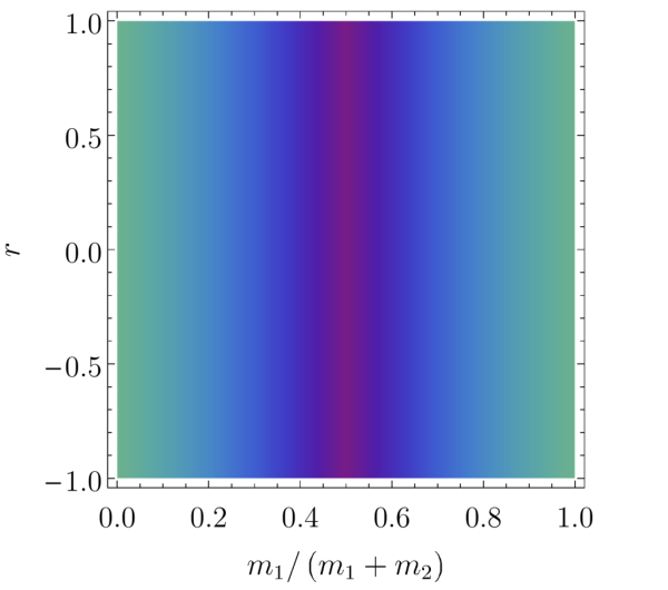
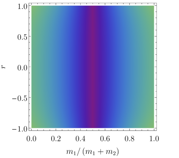
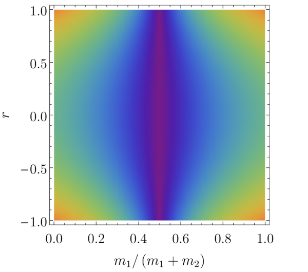
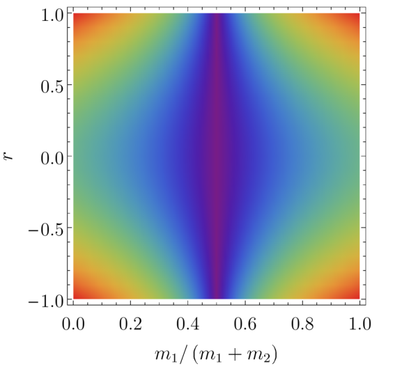
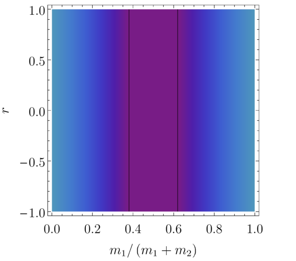
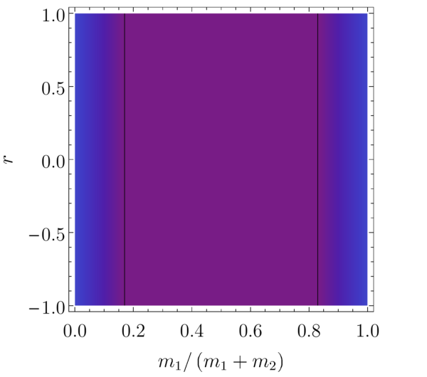
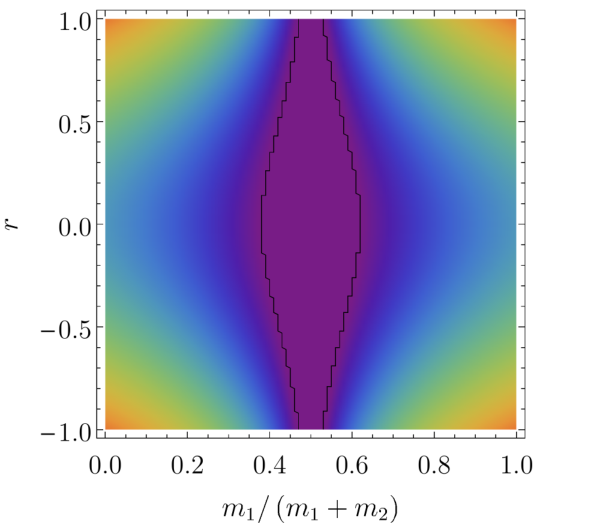
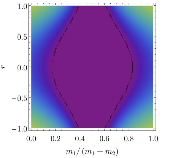
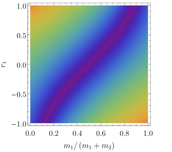
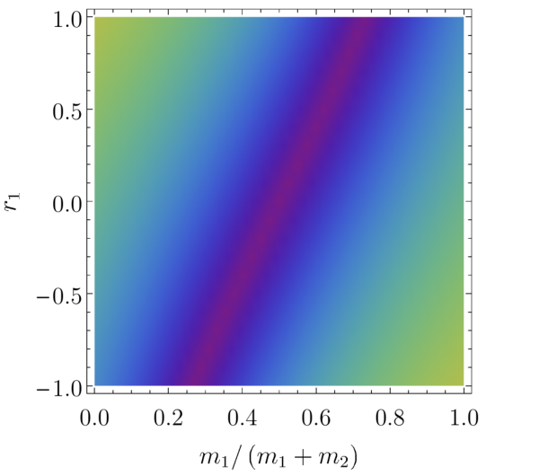
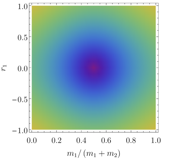
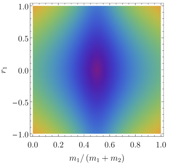
Plots of the logarithmic negativity of the state associated with for different choices of and are given in Figs. 1 (identical state parameters), 2 (differing purity), and 3 (differing squeezing). Several trends emerge from a perusal of these figures.
We first note that equal-mass systems suppress entanglement between center of mass and relational degrees of freedom. When particles in the external partition are prepared such that they have identical covariance matrices we find vanishing entanglement in the equal mass case regardless of the amount of squeezing and rotation. This occurs for both pure and mixed situations, respectively illustrated in Figs. 1 and 2. As one of the masses gets larger, center of mass and relational entanglement increases for any fixed value of the squeezing parameter .
The next trend we observe is that phase rotation, corresponding to squeezing along a rotated axis in phase space, appears to play a more important role than squeezing. For a phase rotation we find that center of mass/relational entanglement is insensitive to the amount of squeezing. As increases we see that squeezing plays an increasingly important role, particularly as the ratio of the masses increasingly departs from unity. Not surprisingly, entanglement is greater for the pure case, shown in Fig. 1, than for the mixed case, shown in Fig. 2.
Asymmetric squeezing (), illustrated in Fig. 3, modifies this situation somewhat. The zero-squeezing case in Figs. 3a and 3b, shows vanishing entanglement when the masses are equal. However there is increased center of mass/relational entanglement as the lighter particle is more strongly squeezed (Fig. 3a), a trend that is less pronounced as the differential squeezing decreases (Fig. 3b). Vanishing center of mass/relational entanglement takes place for increasingly larger values of the mass of the particle which is most squeezed. Again we see that phase rotation plays a more significant role, restoring (in the maximal case) the symmetry present in the equal mass case (Figs. 3c and 3d). Here we see that a sufficient amount of differential squeezing can eliminate center of mass/relational entanglement entirely (Fig. 3c).
Decreasing the purity of the states of the particles in the external partition, shown in Fig. 2, indicates the same trends as for the pure case (Fig. 1). The main effects of decreased purity are to decrease the overall center of mass/relational entanglement and to widen the range of ratio of masses for which this entanglement vanishes.
III.3 Three particles
We consider now a similar analysis for a system of three particles with masses , , and . When transforming a fully factorized state in the external partition , to the center of mass and relational partition , there will again be entanglement generated between the center of mass and relational degrees of freedom. In addition, there will be entanglement generated among the relational degrees of freedom, a new feature not possible for the two particle system considered above.
The center of mass position and momentum operators, along with the relative position and momentum operators are again defined via Eq. (4). The transformed covariance matrix is given by , where
| (24) |
The relational state of particles 2 and 3 as described by particle 1 is obtained by deleting the first and second rows and columns of . We observe that in the limit when vanishes and the columns and rows of associated with particle 3 are deleted, that is the last two rows and columns, as defined in Eq. (19) is recovered.
We assume the state of the three-particle system in the external partition is a fully factorized Gaussian state with the covariance matrix . For simplicity we restrict ourselves to the case when and , in other words a pure state, with each of the three particles identically squeezed in the same direction.
In Fig. 4 the logarithmic negativity as a measure of entanglement between the center of mass and relational degrees of freedom in is plotted for different choices of . In Fig. 5 the logarithmic negativity between the relational degrees of freedom in is plotted for different choices of .


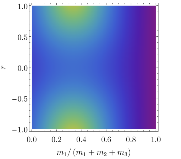

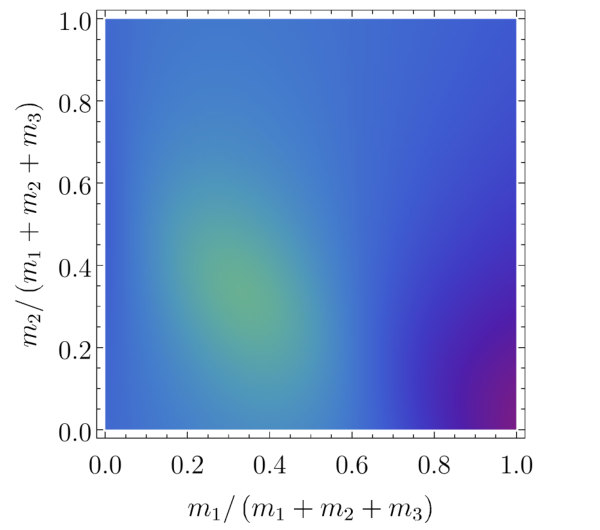
We see similar trends for the center of mass/relational entanglement as for the two-particle case, but qualitatively different behaviour of the internal-relational entanglement, i.e., the entanglement generated among the relational degrees of freedom—in the case at hand, the entanglement between particle 2 and 3 as described by particle 1.
The internal-relational entanglement, illustrated in Fig. 5, shows strikingly different behaviour. Such entanglement is maximized in the equal mass case, shown in Figs. 5b and 5d provided there is some phase rotation. In the absence of phase rotation, this effect vanishes. For all values of the (equal) phase rotation parameter, we observe that as the mass of the reference particle becomes infinite, the entanglement between particles 2 and 3 vanishes. This is as expected, since this limit corresponds to particle 1 behaving as a classical reference frame with a large mass. Indeed, we notice that in the limit , the lower-right submatrix of becomes the identity matrix, and the only effect of the change of coordinates is that of redefining the origin in space for the coordinates of the second and third particle.
IV Discussion and outlook
We have highlighted issues involving quantum reference frames associated with non-compact groups. We began in Sec. II.1 by introducing the usually employed -twirl as a relation description between quantum systems and demonstrated how it leads to unnormalized states when applied to non-compact groups. In Sec. II.2 we saw how the -twirl over the group of translations and Galilean boosts leads to the appearance of the reduced state on the relational degrees of freedom previously considered by Angelo et al. [1]. We then examined the consequences of this relational description in Sec. III by studying the entanglement that emerges between the center of mass degrees of freedom and the relational degrees of freedom, as well as the entanglement among the relational degrees of freedom, for a system of particles, when moving from a description of the quantum system entirely with respect to an external frame, to a description in which only the center of mass is specified with respect to an external frame and all other degrees of freedom are relational.
Two main observations emerged from studying the reduced state on the relational degrees of freedom, introduced in Eq. (10), for systems of two and three particles. First, for fully separable Gaussian states in the external partition with identical second moments, entanglement between the center of mass degrees of freedom and relational degrees of freedom is minimized when the masses of the particles are the same. Second, again for fully separable Gaussian states in the external partition with identical second moments, in the limit when the mass of the reference particle, that is the particle for which the relational degrees of freedom are defined with respect to, becomes infinite, the entanglement among the relational degrees of freedom vanishes. This second observation suggests a meaningful way to interpret the external reference frame, with which we usually describe a quantum state with respect to, as the limit of a physical system, say a particle, in which its mass is taken to infinity [22]. The consequences of this second observation will be explored in future work.
The primary motivation for examining quantum reference frames associated with non-compact groups is to apply the quantum reference frame formalism to relativistic systems, in which the natural group associated with changes of a reference frame is the Poincaré group. It will be fruitful to explore to what extent the tools developed in this manuscript can be applied to the Poincaré group; however, one immediate obstacle is the problem of defining a covariant definition of the center of mass [23].
Two other possible applications of the formalism introduced come to mind. The first is in constructing a relativity principle for quantum mechanics by studying changes of quantum reference frames, which was first suggested in Ref. [14]. The second is to construct a relational quantum theory, similar to what was done in Ref. [10], for the Galilean group using the relational description in Eq. (10), and examine how the usual “non-relational” theory emerges.
Acknowledgements.
The authors would like to thank Nick Menicucci, Jacques Pienaar, and Daniel Terno for useful discussions. This work was supported in part by the Natural Sciences and Engineering Research Council of Canada, by the European Union’s Horizon 2020 research, and innovation programme under the Marie Sklodowska-Curie grant agreement No. 661338. AS and MP acknowledge the hospitality of Macquarie University, where part of this work was conducted.*
Appendix A Purity of the relational state
The covariance matrices considered in sections III.2.1 and III.2.2 were of the form , where both and were given by Eq. (18). The purity of is given by
| (25) |
where and are the purities associated with and respectively.
The purity of the relational state in Eq. (20), that is the state obtained from by taking the partial trace over the center of mass degrees of freedom, is
| (26) |
where we have introduced the notation .
If is pure, which corresponds to both and being pure, then and is a genuine measure of entanglement between the center of mass and relational degrees of freedom. In this case, simplifies to
| (27) |
If the mass of the two particles are equal , further simplifies to
| (28) |
For the case when , and , corresponding to Fig. 1, becomes
| (29) |
From Eq. (29), we observe that when the masses of the two particles are identical , the reduced state is pure, i.e, , which corresponds to vanishing entanglement between the center of mass and relational degrees of freedom in . This agrees with the plots of the logarithmic negativity in Fig. 1.
When the mass of either particle becomes infinite we find
| (30) |
References
- [1] R. M. Angelo, N. Brunner, S. Popescu, A. J. Short, and P. Skrzypczyk, J. Phys. A: Math. Theor. 44, 145304 (2011).
- [2] S. D. Bartlett, T. Rudolph, and R. W. Spekkens, Rev. Mod. Phys. 79, 555 (2007).
- [3] M. Jarzyna and R. Demkowicz-Dobrzański, Phys. Rev. A 85, 011801 (2012).
- [4] S. D. Bartlett, T. Rudolph, R. W. Spekkens, and P. S. Turner, New J. Phys. 11, 063013 (2009).
- [5] A. Kitaev, D. Mayers, and J. Preskill, Phys. Rev. A 69, 052326 (2004).
- [6] Y. Aharonov and L. Susskind, Phys. Rev. 155, 1428 (1967).
- [7] M. R. Dowling, S. D. Bartlett, T. Rudolph, and R. W. Spekkens, Phys. Rev. A 74, 052113 (2006).
- [8] C. Rovelli, Class. Quantum Grav. 8, 317 (1991).
- [9] C. Rovelli, Int. J. of Theor. Phys. 35, 1637 (1996).
- [10] D. Poulin, Int. J. Theor. Phys. 45, 1189 (2006).
- [11] J. Pienaar, (2016), arXiv:1601.07320 .
- [12] A. Chȩcińska and A. Dragan, Phys. Rev. A 92, 012321 (2014).
- [13] I. Marvian and R. B. Mann, Phys. Rev. A 78, 022304 (2008).
- [14] M. C. Palmer, F. Girelli, and S. D. Bartlett, Phys. Rev. A 89, 052121 (2014).
- [15] M. Ahmadi, A. R. H. Smith, and A. Dragan, Phys. Rev. A 92, 062319 (2015).
- [16] G. Adesso and F. Illuminati, J. Phys. A: Math. Theor. 40, 7821 (2007).
- [17] C. Weedbrook, S. Pirandola, R. ́l Garc ́ıa Patro ́n, N. J. Cerf, T. C. Ralph, J. H. Shapiro, and S. Lloyd, Rev. Mod. Phys. 84, 621 (2012).
- [18] G. Adesso, S. Ragy, and A. R. Lee, Open Syst. Inf. Dyn. 21, 1440001 (2014).
- [19] J. Williamson, Amer. J. Math. 58, 141 (1936).
- [20] G. Vidal and R. F. Werner, Phys. Rev. A 65, 032314 (2002).
- [21] G. Adesso, A. Serafini, and F. Illuminati, Phys. Rev. Lett. 93, 220504 (2004).
- [22] Y. Aharonov and T. Kaufherr, Physical Review D 30, 368 (1984).
- [23] P. Aguilar, C. Chryssomalakos, H. H. Coronado, and E. Okon, Int. J. Mod. Phys. A 28, 1350146 (2013).