The role of grain dynamics in determining the onset of sediment transport

There have been a number of approaches aimed at explaining the shape of the Shields curve (see Dey [4] for a comprehensive treatment). To date, the most successful descriptions are hydraulic or empirical scaling formulas [13, 25, 22, 26, 23, 27]; see Paphitis [28] for a review of these models. This approach was pioneered by Shields [13], who originally found that $\Theta_{c}$ varies with ${\rm Re}_{*}$ and noted that ${\rm Re}_{*}$ controls the ratio of the boundary roughness (set by the grain size $D$) to the size of the viscous sublayer. The Shields curve can then be broken into regions where grains are, as compared to the viscous sublayer, completely submerged (${\rm Re}_{*}<2$), near the top ($2<{\rm Re}_{*}<10$), partially protruding ($10<{\rm Re}_{*}<1000$), and fully protruding (${\rm Re}_{*}>1000$). These regions appear to coincide with distinct regimes of the Shields curve. Others have tried a similar approach, where $\Theta_{c}$ is plotted as a function of different nondimensional parameters. For instance, the Yalin number $\Xi={\rm Re}_{*}/\sqrt{\Theta_{c}}$ [26] and dimensionless grain diameter $D_{*}=D(g^{\prime}/\nu^{2})^{1/3}$ [27], where $g^{\prime}=\frac{\rho_{g}-\rho_{f}}{\rho_{g}}g$ is the buoyancy-reduced gravitational acceleration, have been used to eliminate the shear stress dependence on the horizontal axis. These approaches have the advantages of being based in grain scale fluid mechanics and being highly predictive, but they still require an empirical fit to the data shown in Fig. 1.

Attempts at a more theoretical derivation [29, 24, 30, 31, 32] of the shape of the Shields curve are typically based on static force and torque balance of a typical grain that resides on the surface of the bed (see [4] for a thorough review). Such approaches have been successful at capturing certain features of the Shields curve, but not the quantitative shape over the full range of ${\rm Re}_{*}$. Thus, the variation of $\Theta_{c}$ with ${\rm Re}_{*}$ is assumed to be a purely fluid-driven effect. The Shields curve denotes the maximum stress at which a grain on the bed surface in a typical geometric configuration remains in static equilibrium given the ${\rm Re}_{*}$-dependent contributions from lift, drag, and turbulence. However, since these calculations consider a single grain in a particular local environment, they are highly sensitive to the details of that environment, which is often called a “pocket” with pocket angles $\psi$ that specify the orientation of grain-grain contacts [33, 34, 35, 36].

A notable example of this approach by Wiberg and Smith [24] considered a quasi-two-dimensional case where a grain sits in a pocket and motion is initiated when the downstream forces exceed the resistive forces. That is, grain motion occurs when the ratio of the downstream force applied by the fluid on the grain $F_{d}$ to the vertical forces $F_{g^{\prime}}-F_{l}$ (the buoyancy reduced gravitational force minus fluid-induced lift force) are equal to $\cot\psi$ (see Fig. 2). Thus, initiation of motion occurs when

where the subscript $c$ denotes the critical condition to initiate motion. The only inputs to the calculation are the pocket angle $\psi$ (see Fig. 2) and the form of the fluid flow at varying ${\rm Re}_{*}$, which modulates the ratio $(F_{l}/F_{d})_{c}$ and causes variation in $\Theta_{c}$. Wiberg and Smith [24] assumed a logarithmic fluid profile for ${\rm Re}_{*}>100$ and a form proposed by Reichardt [37] for ${\rm Re}_{*}<100$ that has been shown to agree well with experiments [38]. They assumed a drag force $F_{d}=C_{d}\frac{1}{2}\rho_{f}\bar{u}^{2}A_{x}$ and lift force $F_{l}=C_{l}\frac{1}{2}\rho_{f}(\bar{u}_{t}^{2}-\bar{u}_{b}^{2})A_{x}$, where $C_{d}$ is the ${\rm Re}_{p}$-dependent drag coefficient, $\bar{u}$ is the height-dependent velocity profile, subscripts $t$ and $b$ denote the respective values at the top and bottom of the grain, $A_{x}$ is the cross-sectional (frontal) area of a grain, and $C_{l}$ is a constant lift coefficient. They then self-consistently solved Eq. (1) by calculating $F_{d}$ and $F_{l}$ from the appropriate fluid profiles at different values of ${\rm Re}_{*}$. Small grains (${\rm Re}_{*}\ll 1$) are buried deep in the viscous sublayer, and lift forces are small. As ${\rm Re}_{*}$ increases, grains begin to protrude out of the viscous sublayer, and lift forces increase rapidly compared to drag forces. This regime corresponds to the global minimum in the Shields curve at ${\rm Re}_{*}\approx 10$. Large grains (${\rm Re}_{*}\gg 10$) protrude far into the overlying logarithmic flow profile. In this case, lift forces persist, but their effect becomes less pronounced relative to the drag force. In Fig. 1, we show a solution to this equation taken from Wiberg and Smith [24], where the bed roughness $k_{s}$ is equal to the grain diameter $D$ and $\psi=30^{\circ}$. This curve captures the global minimum in the Shields curve at ${\rm Re}_{*}\approx 10$, corresponding to conditions where the grain size is roughly equal to the size of the viscous sublayer. The overall magnitude of this curve is proportional to $\cot\psi$, which is essentially a fit parameter and is very sensitive to the local grain geometry. This curve agrees well with data for ${\rm Re}_{*}>1$, but it underestimates $\Theta_{c}$ at low ${\rm Re}_{*}$. A smaller value of $\psi$ would better capture the data at low ${\rm Re}_{*}$, but there is no clear physical reason to choose a different $\psi$ for small ${\rm Re}_{*}$.

However, a theoretical description for $\Theta_{c}({\rm Re}_{*})$ that includes ${\rm Re}_{*}$-dependent grain dynamics may be able to explain how beds could be stronger at low ${\rm Re}_{*}$. For example, grain motion can be temporary, as individual grains that are unstable at a particular shear force can find more stable locations. Depending on the preparation history of the bed, grains may move initially when a shear flow is applied, but the bed may grow stronger as grains search and find more stable configurations [33, 39, 40, 41]. That is, mobilized grains can often find a more stable pocket than the original one and stop moving, and this effect is usually neglected in prior theoretical considerations. How does ${\rm Re}_{*}$ affect the dynamics of grains as they search for stability? How do the results of models that include the grains’ search for collective stability compare to the Shields curve? This manuscript will address these two important questions.

To illustrate the effects of ${\rm Re}_{*}$-dependent grain dynamics, we first consider a simple example of a grain sitting on top of a 2D bed, shown in Fig. 2. Grain $i$ will become unstable when the ratio of the horizontal fluid force (rightward) and vertical forces (gravity minus lift forces) is $\cot\psi$. After this grain becomes unstable (i.e., not in force and torque balance) at the surface of the bed, the subsequent dynamics depend strongly on ${\rm Re}_{*}$. The mobilized grain can then land and remain in one of the other pockets on the bed surface, labeled 1-3, depending on geometry, grain properties, and the amount of momentum it has acquired. That is, for the grain to land in one of the pockets, the grain must be stable in that pocket at the given $\Theta$ and it must be moving sufficiently slowly to stop in the pocket.

If we approximate the motion of a mobile grain as that of a sphere in a uniform fluid flow, then the drag force is given by $F_{D}=\frac{1}{2}C_{d}\rho_{f}A_{x}V^{2}$, where $A_{x}=\frac{\pi}{4}D^{2}$ is the cross sectional (frontal) area of the sphere, the drag coefficient $C_{d}\approx\frac{24}{\rm{Re}_{p}}+0.4$, the particle Reynolds number ${\rm Re}_{p}=VD/\nu$, and $V$ is the slip velocity between the fluid and the sphere. The first term, $24/{\rm Re}_{p}$, in $C_{d}$ captures Stokes drag (linear in $V$) and the second term, 0.4, captures inertial drag (quadratic in $V$). The dynamics can thus be written as

where $\rho_{g}\frac{\pi}{6}D^{3}$ is the grain mass. The solution to this equation is

where $\tau_{\nu}\propto\frac{\rho_{g}D^{2}}{\rho_{f}\nu}$ is the viscous equilibration time scale, ${\rm Re}_{p}^{0}=V_{0}D/\nu$ is the initial particle Reynolds number, and $V_{0}$ is the slip velocity at $t=0$. If ${\rm Re}_{p}^{0}\ll 1$, then $V(t)=V_{0}\exp(-t/\tau_{\nu})$, and the viscous time scale specifies the dynamics. If ${\rm Re}_{p}^{0}\gg 1$, then $\tau_{\nu}$ becomes large, and a Taylor expansion of the exponential terms in Eq. (3) yields $V(t)=V_{0}\left(1+\frac{t}{\tau_{I}}\right)^{-1}$, where $\tau_{I}\propto\frac{\rho_{g}D}{\rho_{f}V_{0}}$. This solution is also obtained by integrating Eq. (2) with the Stokes drag term set to zero. We note that even for ${\rm Re}_{p}^{0}\gg 1$, $\tau_{\nu}$ still dominates the final portion of the dynamics.

Assuming a constant acceleration $\Theta g^{\prime}$, the dimensionless shear stress $\Theta$ takes a characteristic time $\tau_{\Theta}\propto\sqrt{\frac{D}{\Theta g^{\prime}}}$ to accelerate a grain through a distance $D$, which is the typical spacing between successive collisions with the bed. Here, $g^{\prime}$ is the buoyancy-reduced gravitational acceleration, so $\Theta g^{\prime}$ is the typical acceleration that a grain first experiences after it becomes unstable. We note that $\tau_{\Theta}$ can also be written as $\tau_{\Theta}\propto\sqrt{\frac{\rho_{g}}{\rho_{f}}}\frac{D}{u_{*}}$. The form we have chosen emphasizes its connection to horizontal acceleration of grains along the bed surface. However, the acceleration of a mobile grain will eventually be cut off by equilibrating to the fluid flow. Thus, the bed collision time scale $\tau_{\Theta}$ should be compared to the fluid equilibration time scales $\tau_{\nu}$, which is associated with the viscous component of the drag force, and $\tau_{I}$, which is associated with the inertial component of the drag force. It can be shown that ${\rm Re}_{*}$ compares the viscous equilibration time scale to the bed collision time scale,

For ${\rm Re}_{*}\ll 1$, a weakly mobilized grain quickly equilibrates to the fluid flow. Thus, it is not significantly accelerated between interactions with the bed, it acquires very little momentum, and its dynamics are viscous-dominated. In this case, the effect of grains bouncing over geometrically stable pockets should be negligible. If the grain finds a geometrically stable location, it will stop. When ${\rm Re}_{*}\gg 1$, a mobilized grain is accelerated between successive interactions with the bed, acquiring momentum $p\sim\Theta mg^{\prime}\tau_{\Theta}$, and its dynamics are acceleration-dominated. For ${\rm Re}_{*}\gg 1$, the inertial time scale is dominant, meaning that $\tau_{I}/\tau_{\Theta}$ is the relevant ratio, instead of $\tau_{\nu}/\tau_{\Theta}$. This ratio is a constant, $\tau_{I}/\tau_{\Theta}=\sqrt{\rho_{g}/\rho_{f}}$. Physically, this means that further increasing ${\rm Re}_{*}$ does not cause the grains to be accelerated for longer times. However, a typical ratio $\rho_{g}/\rho_{f}\approx 3$ for rocks, minerals, and soils still yields $\tau_{I}>\tau_{\Theta}$. This means that, for ${\rm Re}_{*}\gg 1$, weakly mobilized grains are significantly accelerated between interactions with the bed [42, 43], which is not true at ${\rm Re}_{*}\ll 1$. This framework provides a mechanism whereby grains stop more easily at low ${\rm Re}_{*}$ than at high ${\rm Re}_{*}$, given the same value of $\Theta$. Note that this argument implies that $\tau_{I}$ plays a secondary role, and that much of the relevant physics can be captured by a viscous drag law, neglecting the inertial component. We return to this point in our argument below. We also note that our dimensional analysis focuses on a comparison of a viscous damping time $\tau_{\nu}$ to an acceleration time scale $\tau_{\Theta}$. This is similar in spirit to a Stokes number [44, 45, 46], which plays a crucial role in the degree of energy loss in fluid-mediated grain-grain collisions. To compare to the data in Fig. 1, we chose to formulate our results in terms of ${\rm Re}_{*}$.

To test this interpretation, we here present the results of discrete-element method (DEM) simulations. While many DEM-based approaches include as much physical realism as possible [47, 48, 49, 50, 51], we here simplify the problem to isolate the role of ${\rm Re}_{*}$ as the ratio of the two time scales controlling grain dynamics. Thus, we are neglecting many physical effects such as ${\rm Re}_{*}$-dependent lift forces [24], cohesive forces [52], turbulent fluctuations [43, 53], coherent structures [54, 55, 56, 57], added mass forces [58], and Basset forces [59]. In the present study, noncohesive grains are driven by a model fluid shear flow, which does not vary with ${\rm Re}_{*}$, but is coupled to the velocity of the grains through a drag law, which sets ${\rm Re}_{*}$. In previous work [60], we investigated how $\Theta_{c}$ varied with a particle Reynolds number using a purely linear drag law in 2D with frictionless, purely elastic grain-grain interactions. Interestingly, even this simple model captured certain features of the Shields curve, namely plateaus at low and high particle Reynolds number with a decrease in between. In this work, we use the improved dimensional analysis presented above to explicitly connect the form of the drag law to ${\rm Re}_{*}$, in order to more directly compare the results of the DEM simulations to the Shields curve. Additionally, we vary the spatial dimension (2D to 3D), inelastic grain-grain interactions, friction, irregular grain shape, and the form of the drag law (linear to quadratic). We also include ${\rm Re}_{*}$-independent lift forces and vary their magnitude. By varying these parameters, our goal is to understand the minimal subset of parameters that control the shape of $\Theta_{c}({\rm Re}_{*})$ from the perspective of ${\rm Re}_{*}$-dependent grain dynamics.

We study systems composed of $N/2$ large and $N/2$ small grains with diameter ratio $1.4$ in 2D [61, 62] and $1.2$ in 3D [63]. These size ratios are chosen to maintain structural disorder in the bed. In our analysis, we use the average diameter to evaluate dimensionless quantities such as ${\rm Re}_{*}$. Our domain has periodic boundaries in the stream-wise direction, as well as in the cross-stream direction in 3D. We use no upper confining boundary and a rigid lower boundary with infinite friction so that the horizontal velocities of all grains touching it are fixed to zero. We integrate Newton’s equations of motion for each grain, including rotational and translational degrees of freedom, using a sixth-order Gear predictor-corrector integration scheme for the case of Cundall-Strack friction [64] for disks in 2D and a modified velocity Verlet integration scheme for all other systems. The total force on each grain is given by the vector sum of contact forces from other grains, a gravitational force, and a drag force from a fluid that moves horizontally, so that

The total torque on each grain is only due to tangential contact forces, so that

Here, the sum over $j$ only includes grains contacting grain $i$, $\vec{s}_{ij}$ is the vector connecting the center of grain $i$ to the point of contact between grains $i$ and $j$, $m_{i}$ is the mass of the grain ($m_{i}\propto D_{i}^{2}$ in 2D and $m_{i}\propto D_{i}^{3}$ in 3D), $I_{i}$ is the moment of inertia of the grain, $D_{i}$ is the diameter of the grain, $\vec{v}_{i}$ is the velocity of the grain, $m_{i}g^{\prime}$ is the buoyancy-corrected grain weight, $\hat{z}$ is the upward normal vector, and $\vec{F}_{f}$ is the drag force from a model fluid flow, which we discuss below. For the frictionless, elastic case [60], $\vec{F}^{c}_{ij}=\vec{F}^{r}_{ij}$, where $\vec{F}^{r}_{ij}=K\left(1-\frac{r_{ij}}{D_{ij}}\right)\theta\left(1-\frac{r_{ij}}{D_{ij}}\right)\hat{r}_{ij}$ is the pairwise (linear repulsive spring) force on grain $i$ from grain $j$, where $K$ is the grain stiffness, $r_{ij}$ is the separation between the centers of the grains, $D_{ij}=(D_{i}+D_{j})/2$, $\hat{r}_{ij}$ is the unit vector connecting their centers, and $\theta$ is the Heaviside step function. We set the nondimensional stiffness $\frac{K}{mg^{\prime}}>3\times 10^{3}$ to be sufficiently large that our results become independent of $K$. In this study, we modify the contact force $\vec{F}^{c}_{ij}$ to include dissipative grain-grain interactions and tangential forces. The dissipative force is given by $\vec{F}^{d}_{ij}=\gamma_{v}\frac{m_{i}m_{j}}{m_{i}+m_{j}}(\vec{v}_{i}-\vec{v}_{j})\cdot\hat{r}_{ij}$, where the dissipation rate $\gamma_{v}=\frac{-2\log e_{n}}{\tau_{c}}$, $\tau_{c}=\frac{\pi\sqrt{m}}{2K}$ is the grain-grain collision time, $m$ is the mean grain mass, and $e_{n}$ is the coefficient of normal restitution [65]. This form for the normal dissipation is often used to model energy losses that arise from contact mechanics, such as viscoelasticity, internal heating, or internal vibrational modes of grains. Here, it is likely that the fluid in the intergrain gap dominates the energy loss during a collision, and the effective $e_{n}$ depends on the relative impact velocity of the grains and the viscosity of the fluid via the Stokes number ${\rm St}=\frac{\rho_{g}v_{ij}D}{\rho_{f}\nu}$ [45, 44, 46, 59], where $v_{ij}$ is a relative velocity between colliding grains. We hold $e_{n}$ fixed for each individual simulation, independent of the relative grain velocity at contact or local fluid behavior. We will include velocity and viscosity dependence of the coefficient of restitution in future studies. Tangential forces in granular beds arise via two mechanisms: nonspherical grain shape and microscopic friction. We approximate these two mechanisms using a grain-asperity model [66, 67], shown in Fig. 3(b), and the Cundall-Strack model for friction [64], shown in 3(c). Further details are provided in Appendix A.

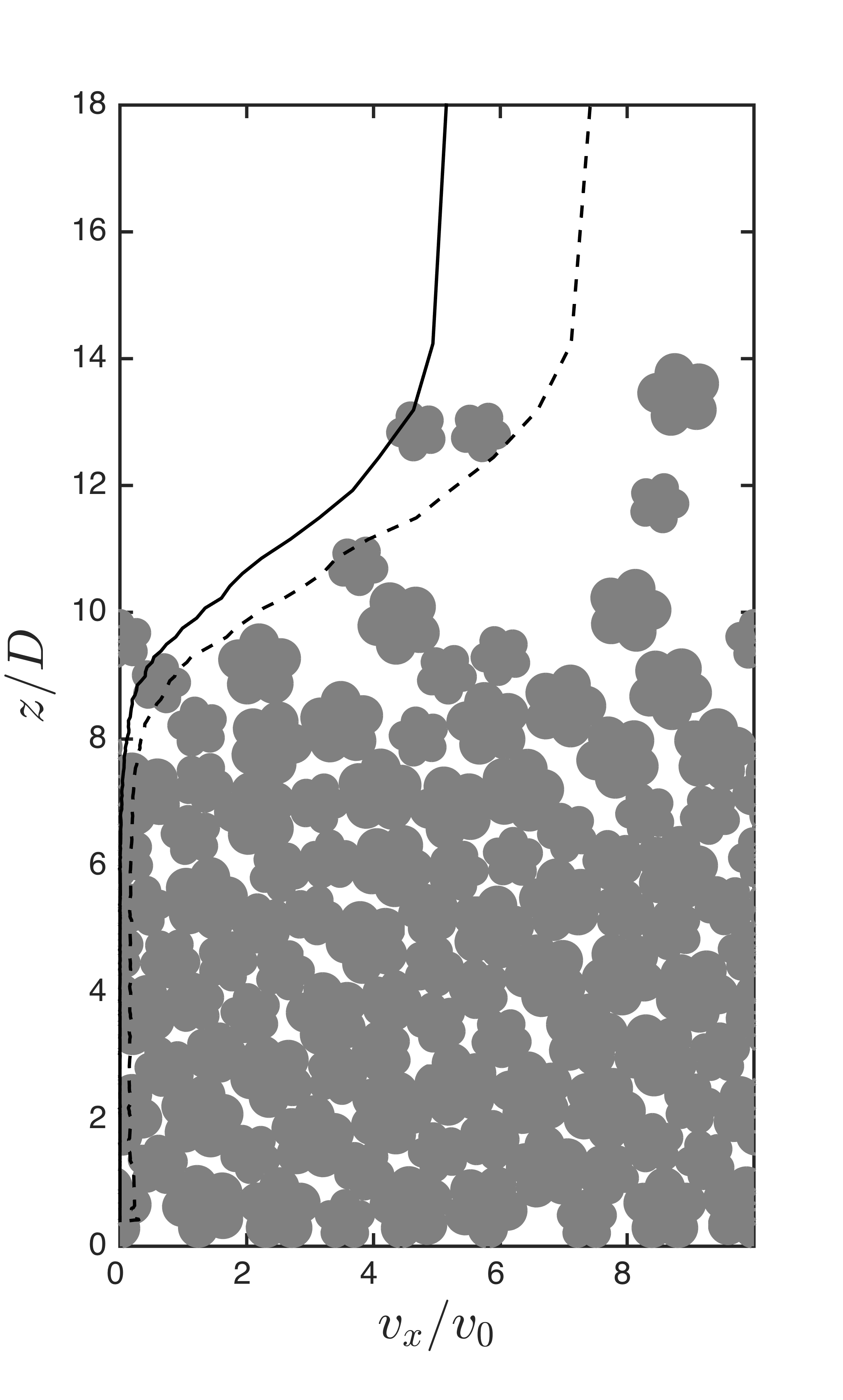
To simulate fluid shear, we choose a model fluid velocity profile that acts primarily on the surface grains of a static bed and that increases somewhat for mobilized grains that move above the surface. We set a characteristic fluid velocity $v_{0}$ at the surface of a static bed, and we multiply this velocity by a fluid profile $f(\phi_{i})$, where $\phi_{i}$ is the local packing density at grain $i$, which yields $v_{0}f(\phi_{i})$ acting on grain $i$. Our simulations use the local packing fraction $\phi_{i}$, which varies horizontally and vertically, but our results are insensitive to horizontally averaging $\phi_{i}$ such that local packing fraction only varies vertically. In 2D, $f(\phi_{i})=e^{-b(\phi_{i}-\phi_{t})}$, where $b$ controls the ratio of the magnitude of the fluid flow above and inside the bed and $\phi_{t}=0.5$ is the typical packing fraction of a grain at the top of a static 2D bed. $\phi_{i}$ is calculated in a small region with diameter $D_{i}+2D_{l}$ around the center of each grain, where $D_{l}$ is the diameter of the larger grains. Since $f=1$ for $\phi_{i}=\phi_{t}$, $v_{0}$ is roughly equal to the fluid velocity at the free granular surface. In 3D, we use a modified form, $f(\phi_{i})=[\exp(-b\phi_{i})-\exp(-b\phi_{m})]/[\exp(-b\phi_{t})-\exp(-b\phi_{m})]$, as shown in Fig. 4. $\phi_{m}=0.7$ approximates the maximum packing fraction in the bulk of the bed, and $\phi_{t}=0.42$ is a typical packing fraction of a grain at the top of the bed. This modified form is used to sufficiently reduce the fluid velocity inside a 3D bed, where typical packing fractions are much smaller ($\approx 0.55-0.64$) than in 2D ($\approx 0.75-0.84$). For all simulations, we set $b=5$. We find that our results are insensitive to the choice of $f$, provided its magnitude is very small in the bed. Since $\phi_{t}$ causes a shift in our definition of the height of the bed surface (see Fig. 4), varying this parameter corresponds to multiplying all our results for $\Theta$ by an order unity prefactor. However, our results are qualitatively unaffected by this choice, and quantitative variation is weak, provided the choice for $\phi_{t}$ falls within a reasonable range taken from Fig. 4 (i.e., 0.35 – 0.5)

To add model lift forces (in 3D only), we consider the difference $\Delta\phi_{i}$ in packing fraction between the top and bottom of a grain (Fig. 4). We again calculate the packing fraction in a small region with diameter $D_{i}+2D_{l}$ around the top and bottom of each grain, and $\Delta\phi_{i}$ is the difference between these two quantities. $\Delta\phi_{i}$ is small in the bulk of a bed, large at the bed surface, and small for mobilized grains above the bed. We then define a lift profile $l(\Delta\phi_{i})=\frac{\Delta\phi_{i}}{0.3}$, where the factor 0.3 is chosen to normalize $l$ to unity at the bed surface.

We then set the fluid force $\vec{F}_{f}$ from Eq. (5) equal to the form from Eq. (2),

where $B_{1}=3\pi\rho_{f}\nu D_{i}$ and $B_{2}=\frac{\pi}{20}\rho_{f}D_{i}^{2}$, and $B_{l}$ is a lift coefficient. While there are two different particle diameters, we use the mean value $D$ in our dimensional analysis below. In addition to $\frac{K}{mg^{\prime}}$, $\mu$, and $e_{n}$, which determine grain-grain interactions, Eqs. (5)-(7) include four additional nondimensional numbers:

$\Theta$ is the Shields parameter, where the factor $2/3$ from Eq. (1) represents a conversion [24] from a force ratio [i.e., in Eq. (8), $B_{1}v_{0}$, $B_{2}v_{0}^{2}$, and $mg^{\prime}$ have units of force] to the stress ratio $\Theta=\frac{\tau}{\rho g^{\prime}D}$. Assuming that the fluid stress $\tau$ acts approximately over the cross-sectional area of a sphere, $A=\frac{\pi}{4}D^{2}$, then $\tau A$ is the horizontal force exerted on a static grain. The gravitational stress $\rho g^{\prime}D$ acts over an effective area $\frac{V}{D}=\frac{\pi}{6}D^{2}$, and $\rho g^{\prime}D\frac{V}{D}$ is the grain weight. Thus, the explicit force ratio $\frac{B_{1}v_{0}+B_{2}v_{0}^{2}}{mg^{\prime}}$ is converted to a stress by multiplying by $\frac{V}{AD}=\frac{2}{3}$. In Eq. (9), we rewrite the shear Reynolds number ${\rm Re}_{*}=\sqrt{\frac{\rho_{f}}{\rho_{g}}}\frac{\tau_{\nu}}{\tau_{\Theta}}$ from Eq. (4) in Sec. I.2 in terms of parameters relevant to the simulations [see Eq. (7) using $\tau_{\nu}=m/B_{1}$, $\tau_{\Theta}=\sqrt{\frac{D}{\Theta g^{\prime}}}$, and $\rho_{g}/\rho_{f}=\sqrt{3}$]. These two forms in Eqs. (4) and (9) are equivalent, and both reduce to the standard form ${\rm Re}_{*}=\frac{u_{*}D}{\nu}$. Next, ${\rm Re}_{p}^{0}$ is the particle Reynolds number of a grain at the surface of the bed, which determines the relative contributions of the viscous and inertial drag terms. We emphasize that, when comparing results between a linear drag law, where $B_{2}=0$, and a quadratic drag law, where $B_{2}/B_{1}$ is determined by ${\rm Re}_{p}$ according to Eq. (10), we first assign $\Theta$ and then specify $v_{0}$. Simulations for linear and quadratic drag laws at the same $\Theta$ will require different values of $v_{0}$. This is distinct from the case where the fluid velocity is specified, in which case we would severely underestimate the stresses at high ${\rm Re}_{*}$. Finally, $\frac{F_{l}}{F_{d}}$ represents the characteristic ratio of lift to drag forces at the bed surface. We set this quantity to zero in all but a small number of our simulations.

To characterize the onset and cessation of bed motion in our system, we employ two protocols. To study the mobile-to-static (M-S) transition defined by $\Theta_{c}$, we distribute all grains randomly on a cubic lattice throughout the domain and set a constant value of $\Theta$ for a total time of roughly $10^{6}$ grain-grain collision times (our results are insensitive to the details of this initial condition, as long as we consider large ensembles of initial conditions where a significant fraction of grains are suspended when the model fluid flow is applied). We then observe if and when our system stops, which we define as when the maximum acceleration $a_{\rm max}<a_{\rm thresh}$ and maximum velocity $v_{\rm max}<v_{\rm thresh}$, where $a_{\rm thresh}$ is roughly one order of magnitude smaller than $g^{\prime}$ and roughly three orders of magnitude smaller than typical values for a moving bed and $v_{\rm thresh}$ is roughly three orders of magnitude smaller than the fluid velocity at the surface. Our results are independent of the values of these thresholds, provided they are sufficiently small. To understand the dynamics of the static-to-mobile (S-M) transition, we begin with a static bed and slowly increase $v_{0}$ in small increments, corresponding to increases in stress $\Delta\Theta\leq 0.05\Theta$ until we observe $a_{\rm max}>a_{\rm thresh}$ or $v_{\rm max}>v_{\rm thresh}$. We then keep $v_{0}$ constant until $a_{\rm max}<a_{\rm thresh}$ and $v_{\rm max}<v_{\rm thresh}$ or until the end of our simulation. Table 1 gives a full list of the parameter values we explore, and we refer back to each of these settings S-1 through S-8 throughout the remainder of the manuscript.

We present our results in the following way. In Sec. III.2, we show simulations in 3D using a quadratic drag law (S-1 settings in Table 1). We show that $\Theta_{c}({\rm Re}_{*})$ from this model mimics the Shields curve. Quantitative discrepancies are consistent with the relative contribution of lift forces [24], as well as possible contributions from turbulent fluctuations [54, 53, 56, 43] and coherent structures [55, 57]. We also find that $\Theta_{c}({\rm Re}_{*})$ is identical for both a quadratic drag law in 3D (S-1 settings) and a linear drag law in 3D with small $e_{n}$ (S-2 settings). We show these results in order to justify our argument in Sec. I.2 that the inertial time scale $\tau_{I}$ plays only a secondary role, since linear drag includes only $\tau_{\nu}$ and not $\tau_{I}$. In Sec. III.3, we give further details of how $\Theta_{c}({\rm Re}_{*})$ with linear drag (S-2 and S-3 settings) converges to the result from quadratic drag (S-1 settings) when $e_{n}$ approaches zero. In Sec. III.4, we include lift forces at the bed surface (S-4 settings), and $\Theta_{c}$ decreases as expected. In Sec. III.5, we use 2D simulations (S-5 and S-6 settings) to show that friction and irregular grain shape only weakly affect the results. In Sec. III.6, we use weakest-link statistics to show that grain motion is always initiated at $\Theta_{c}({\rm Re}_{*})$ for large systems (using S-7 and S-8 settings). This picture suggests that fluid-sheared granular beds possess a dynamical instability for moderate to high ${\rm Re}_{*}$, where mobile grains are unable to stop, and that grain dynamics plays a dominant role in this regime.

The main result from our work is shown in Figure 5. The small, black dots represent experimental and field data from Dey [4]. The black curve with square markers is the boundary $\Theta_{c}({\rm Re}_{*})$ in 3D between systems with and without sustained grain motion from our model with S-1 settings. We find a nearly identical boundary using a linear drag law when $e_{n}$ is small, as shown by the solid blue curve with open circles, where $e_{n}=0.2$ (S-2 settings). As discussed below in Sec. III.3, small $e_{n}$ suppresses the effect of grain impact with the bed for linear drag; for quadratic drag, the inertial equilibration time scale limits the kinetic energy of mobilized grains. In both the cases of linear drag with small $e_{n}$ and quadratic drag, the key physics near $\Theta_{c}$ is the dynamics of mobilized grains between successive interactions with the bed.

Since we do not vary the fluid flow profile, ${\rm Re}_{*}$-dependent grain dynamics are solely responsible for the variation seen in Fig. 5. To illustrate how grain dynamics vary with ${\rm Re}_{*}$, Fig. 6 shows data from simulations of mobilized beds using S-1 settings at $\Theta\approx\Theta_{c}({\rm Re}_{*})$ for $10^{-2}\leq{\rm Re}_{*}\leq 10^{3}$. Figure 6(a) shows height $z/D$ versus packing fraction $\phi_{i}$, and the inset shows the maximum height $z_{\rm max}$ that mobile grains achieve as a function of ${\rm Re}_{*}$. Figure 6(b) shows height $z/D$ versus grain velocity $v_{x}^{g}/v_{0}$ (solid lines) and fluid velocity $v_{x}^{f}/v_{0}$ (dashed lines). The inset shows the ratio of average grain velocity $\bar{v}_{x}^{g}$ in the top layer and above (i.e., $z/D>5.25$) to the average fluid velocity $\bar{v}_{x}^{f}$ in the same region. As ${\rm Re}_{*}$ increases, $\bar{v}_{x}^{g}/\bar{v}_{x}^{f}$ decreases, meaning that mobile grains do not equilibrate to the fluid flow. Figure 6(c) shows the height $z/D$ versus the normalized horizontal grain acceleration $a_{g}(\Theta g^{\prime})^{-1}$. At small ${\rm Re}_{*}$, grain acceleration is negligible, and mobile grains always move with the local fluid flow. At high ${\rm Re}_{*}$ grains are significantly accelerated, and their momentum is lost through collisions with the bed, which is indicated by the negative acceleration peak at the bed surface for ${\rm Re}_{*}\approx 250$ (green stars). The inset shows the average normalized horizontal grain acceleration $\bar{a}_{g}(\Theta g^{\prime})^{-1}$ in the top layer and above ($z/D>5.25$) as a function of ${\rm Re}_{*}$. As ${\rm Re}_{*}$ increases, average normalized horizontal grain acceleration for mobilized grains increases until it plateaus for ${\rm Re}_{*}>10$. Together these data show how grain dynamics vary with ${\rm Re}_{*}$ from viscous-dominated at low ${\rm Re}_{*}$ to acceleration-dominated at high ${\rm Re}_{*}$, as discussed in Sec. I.2.

Our results for $\Theta_{c}({\rm Re}_{*})$ in Fig. 5 display plateaus at low and high ${\rm Re}_{*}$, denoted $\Theta_{c}^{l}$ and $\Theta_{c}^{h}$, respectively. The behavior of the Shields curve at ${\rm Re}_{*}<1$ is currently an open question. Most hydraulic models [22, 23, 28] assume a decreasing trend of $\Theta_{c}({\rm Re}_{*})$ for ${\rm Re}_{*}<10$. In simulations, we observe a plateau [68, 69] with $\Theta_{c}^{l}\approx 0.28$, which numerically agrees with [68] as well as the data shown in Fig. 1. We interpret this plateau as the shear force corresponding to the most geometrically stable arrangement of the bed, suggesting that configurations that can resist $\Theta>\Theta_{c}^{l}$ do not exist. As ${\rm Re}_{*}$ is increased, $\Theta_{c}$ decreases, as grain dynamics begin to transition out of the viscous regime (${\rm Re}_{*}\ll 1$). For ${\rm Re}_{*}\gg 1$, $\Theta_{c}$ also displays a plateau $\Theta_{c}^{h}$ that has the same value for linear and quadratic drag laws. Note that, for a linear drag law, a larger fluid velocity is required to achieve the same $\Theta$ when compared to a quadratic drag law.

The quadratic drag law in Eq. (2) natually includes both $\tau_{\nu}$ and $\tau_{I}$ as defined in Sec. I.2. However, the linear drag law (S-2 and S-3 settings) only includes $\tau_{\nu}$, not $\tau_{I}$. In Sec. I.2, we showed that ${\rm Re}_{*}\propto\tau_{\nu}/\tau_{\Theta}$, and we argued that the inertial time scale $\tau_{I}$ plays a secondary role since it is always longer than $\tau_{\Theta}$ given typical grain and fluid densities. To justify this claim and to connect to our previous work using a linear drag law [60], we show results in this section from 3D simulations with linear (S-3 settings) and quadratic (S-1 settings) drag laws. We show below that $\Theta_{c}({\rm Re}_{*})$ and the sediment transport rates are the same for linear and quadratic drag laws, provided $e_{n}$ is small when a linear drag law is used. If $e_{n}$ is not small, then mobilized grains at ${\rm Re}_{*}\gg 1$ are accelerated over time $\tau_{\nu}$ instead of being cut off by $\tau_{I}$, leading to hysteresis at ${\rm Re}_{*}\gg 1$. We again note that $\Theta$ is set by the typical force felt by surface grains, not by the velocity of the fluid. This means that when comparing linear and quadratic drag at high ${\rm Re}_{*}$, we use larger fluid velocities for the linear case to obtain the same value of $\Theta$, since we are neglecting the quadratic term in the drag laws shown in Eqs. (2) and (7).

Figure 7 shows the boundaries between systems with and without sustained grain motion for quadratic and linear drag laws. The thick black line with square markers shows the boundary between systems with and without sustained grain motion using a quadratic drag law (S-1 settings), representing both the transitions from a mobile to a static bed as well as from a static to a mobile bed (i.e., we observe no hysteresis for a quadratic drag law). This boundary is independent of $e_{n}$. The thin, colored lines with circle markers show the minimum $\Theta$ required to sustain grain motion indefinitely, using a linear drag law (S-3 settings). The different colors (red, green, black, blue, magenta) represent different restitution coefficients ($e_{n}=0.9$, 0.8, 0.5, 0.2, and 0.1). As $e_{n}\rightarrow 0$, these boundaries form a single curve, with plateaus $\Theta=\Theta_{c}^{l}\approx 0.28$ and $\Theta=\Theta_{c}^{h}\approx 0.11$ at low and high ${\rm Re}_{*}$, respectively. Note that Niño and García [59] showed experimentally that restitution coefficients are typically small ($e_{n}<0.5$) for saltating grains rebounding off a sediment bed. The dashed, black line represents $\Theta_{0}^{h}$, which is the minimum $\Theta$ required to initiate sustained grain motion from a static bed at ${\rm Re}_{*}\gg 1$. As we show in Section III.6, sustained grain motion is always initiated at this value in the large-system limit. We find that $\Theta_{0}^{h}$ is insensitive to the drag law and restitution coefficient (i.e., $\Theta_{0}^{h}$ is constant for S-1, S-2, and S-3).

When ${\rm Re}_{*}\ll 1$, the linear (S-2 and S-3 settings) and quadratic (S-1 settings) drag laws agree, and our simulations show identical results. Grain flux tends to zero and stopping times diverge at a critical value $\Theta_{c}^{l}\approx 0.28$. Figure 8 shows representative data for ${\rm Re}_{*}\gg 1$. As discussed in Section II.2, we begin with a mobilized system, where grains are suspended, and apply the model fluid flow. $\Theta_{c}$ is characterized by a grain discharge per unit width that tends to zero and diverging stopping times for $\Theta$ just below $\Theta_{c}$. We characterize the grain motion by plotting $q/\sqrt{g^{\prime}D^{3}}$, where $q$ is the discharge per unit width. The dashed curves in Fig. 8(a) show $q/\sqrt{g^{\prime}D^{3}}$ at different times (blue to red represents increasing time), where each data point is obtained from an ensemble of ten simulations using S-1 settings. Each data point with a nonzero $q$ means that in at least half of the simulations the grains did not stop, and the value of $q$ represents the average of all simulations where grains were still in motion. The solid black curve represents the steady state grain flux (measured at the end of the simulation). If in at least half of the simulations, the grains stopped, we measure the average time $t_{s}$ that it took the grains to stop moving. Figure 8(b) shows $(t_{s}-t_{s,0})\sqrt{g^{\prime}/D}$ plotted versus $\Theta$ for quadratic drag (S-1 settings) and linear drag (S-3 settings). Figure 8(c) shows $q$ versus $\Theta$ for quadratic and linear drag. We find that $q$ tends to zero and $t_{s}$ diverges at roughly the same value of $\Theta$. As $e_{n}\rightarrow 0$ for linear drag, the critical $\Theta$ approaches the value for the quadratic drag law, $\Theta=\Theta_{c}^{h}\approx 0.11$.

Thus, at ${\rm Re}_{*}\gg 1$, we find that using linear (with small $e_{n}$) and quadratic drag laws give the same value of $\Theta_{c}$ as well as the same dependence of $q$ versus $\Theta$. Under a linear (viscous only) drag law, grains can be accelerated to much larger speeds, since $\tau_{\nu}\propto{\rm Re}_{*}$ for all ${\rm Re}_{*}$, and the equilibration time is not cut off by $\tau_{I}$. Thus, in simulations with a linear drag law, mobile grains can deliver significant energy when they impact the bed and can rebound to large heights above the bed from elastic collisions (not lift forces) if $e_{n}$ is large. These effects are suppressed when $e_{n}$ is small and $\Theta$ is near $\Theta_{c}$, and the behavior of $q(\Theta)$ for linear drag approaches the $q(\Theta)$ curve for quadratic drag as $e_{n}\rightarrow 0$. In this case, the trajectory of mobilized grains is confined to positions near the bed, and viscous and inertial drag laws yield the same behavior very close to $\Theta_{c}$.

The results of our model do not quantitatively capture the global minimum in the Shields curve at ${\rm Re}_{*}\approx 10$ and overestimate $\Theta_{c}$ by roughly a factor two at high ${\rm Re}_{*}$. However, in this model we neglected lift forces and turbulence, and thus we expect to overpredict $\Theta_{c}$ in this regime. For instance, the calculation from Wiberg and Smith [24] discussed in Sec. I.1 and shown in Fig. 1 could be combined with our model to capture ${\rm Re}_{*}$-dependent lift forces. To demonstrate the viability of this approach, in this section we show that lift forces decrease $\Theta_{c}$ in a way that is quantitatively consistent with Eq. (1).

Figure 9 shows the results of 3D simulations with quadratic drag and constant lift forces (S-4 settings) which are not ${\rm Re}_{*}$-dependent. We vary $\frac{F_{l}}{F_{d}}$ from 0 to 3, and the corresponding curves $\Theta_{c}\left({\rm Re}_{*},\frac{F_{l}}{F_{d}}\right)$ decrease, as expected. The magnitude of these curves follows the scaling shown in Eq. (1), but where $\cot\psi$ is replaced by $\frac{3}{2}\Theta_{c}\left({\rm Re}_{*},0\right)$, which is the ratio of horizontal to vertical forces required in simulations at varying ${\rm Re}_{*}$:

We reiterate that the model lift forces we include have constant $\frac{F_{l}}{F_{d}}$, whereas physical systems likely have lift forces that vary strongly with ${\rm Re}_{*}$. It is possible that a scaling function $\frac{1}{1+\frac{3}{2}\Theta_{c}\left({\rm Re}_{*},0\right)\frac{F_{l}}{F_{d}}}$ that is directly calculated from the ${\rm Re}_{*}$-dependent fluid forces could by combined with our results to quantitatively recapitulate the Shields curve over the full range of ${\rm Re}_{*}$.

In this section, we use 2D simulations (S-5 and S-6 settings) to show that $\Theta_{c}({\rm Re}_{*})$ is only weakly dependent on friction and irregular grain shape. These results are shown in Fig. 10. In 2D, the numerical values for $\Theta_{c}$ increase by roughly a factor of two. We interpret the increase in $\Theta_{c}$ from 3D to 2D to follow from the fact that the energy landscape of a 2D bed is more difficult for grains to navigate, as grains must roll over obstacles instead of traversing the low points between impeding grains. This raises important questions about whether and how quasi-2D calculations of pocket angles relate to 3D systems.

We perform simulations in 2D with a linear drag law where grain-grain interactions include Cundall-Strack friction (S-5 settings) or geometrical friction from irregular grain shape (S-6 settings). We find hysteresis that vanishes in the limit of small $e_{n}$, as in 3D (Fig. 7), and we plot the small $e_{n}$ values in Fig. 10, which correspond to the result with a quadratic drag law. Figure 10 shows the values of the plateaus $\Theta_{c}^{l}$ and $\Theta_{c}^{h}$ as friction is varied. Circles represent disks with Cundall-Strack friction, with a friction coefficient $\mu$. Other symbols correspond to $n-$mers with $n=2$ (diamonds), 3 (triangles), 4 (squares), and 5 (stars). Both $\Theta_{c}^{l}$ and $\Theta_{c}^{h}$ increase by less than 50% with increasing friction, which is still comparable to the scatter in the experimental and field data shown in Fig. 1. We note that Joseph and Hunt [70] found a friction coefficient of $\mu\approx 0.15$ for submerged spheres, and we observe almost no variation in $\Theta_{c}^{l}$ and $\Theta_{c}^{h}$ for friction coefficients at or below this measured experimental value.

Thus far, we have argued that grain dynamics at varying ${\rm Re}_{*}$ play a dominant role in determining $\Theta_{c}({\rm Re}_{*})$, as opposed to static force and torque balance of individual grains in typical pocket geometries. However, the onset of grain motion must follow from a breakdown of force and torque balance on one or more grains. In this section, we show data (using S-7 and S-8 settings) for the initiation of sustained grain motion (i.e., the static-to-mobile transition), which, in the limit of large systems, always occurs at the same dynamical boundary $\Theta_{c}({\rm Re}_{*})$ that denotes the minimum applied fluid stress at which mobilized systems are unable to stop. We show that local motion in one of many uncorrelated subsystems leads to global sustained grain motion using Weibullian weakest-link statistics [71, 72]. Additionally, we find that the characteristic time $t_{m}$ for the bed to fully mobilize diverges at $\Theta_{c}$, consistent with a dynamical instability at $\Theta=\Theta_{c}$ that is activated by a single mobilized region.

If we consider the bed to be a composite system of $M$ uncorrelated subsystems that begin to move if any of the subsystems move at $\Theta>\Theta_{c}$ (when grain motion will be sustained indefinitely), then the cumulative distribution $C_{M}(\Theta)$ for the initiation of grain motion in the collective system is related to that of a single subsystem $C(\Theta)$ by

By assuming a Weibull distribution for $C(\Theta)$ [71, 72, 73]

then $C_{M}(\Theta)$ in Eq. (13) has the same form with $\alpha_{M}=\alpha$ and $\beta_{M}=\beta M^{-1/\alpha}$. As in our previous study [60], we find that this scaling holds for all systems we have considered here. This means that Eq. (13) applies, confirming that global grain motion is initiated by a single member of a collection of uncorrelated subsystems (i.e., local pockets). In the limit of large system size, we find that grain motion is always initiated at $\Theta_{c}$.

For a given system with static grains, we slowly increase $\Theta$ until sustained grain motion occurs at $\Theta=\Theta_{f}>\Theta_{c}$. Figure 11(a) shows the distributions of the excess stress $\Theta_{f}-\Theta_{c}$ required to initiate sustained grain motion in ensembles of static 3D quadratic-drag systems (S-7 settings) as $\Theta$ is slowly increased. These ensembles are prepared at $\Theta\approx 0.067<\Theta_{c}$ with a fill height of $5D$ and a cross stream width of $4D$, and we vary the stream-wise distance $W/D$ between 2.5 and 40. These distributions collapse when rescaled by their mean, as shown in the inset, with a shape parameter $\alpha\approx 2.2$. This value is comparable to that measured in the frictionless, elastic case, where we found $\alpha\approx 2.6$ [60]. The scaling of mean excess stress $\bar{\Theta}_{f}-\Theta_{c}$, as shown in Figure 11(b), is consistent with a power law scaling with exponent $-1/\alpha$, confirming Eqs. (13) and (14). For systems that fail, we measure the mobilization time $t_{m}$, which we define as the time required for the grain flux $q$ to go from zero to the steady-state value. This quantity is plotted versus $\Theta$ in Fig. 11(c), and it diverges at $\Theta_{c}$, like the divergence of $t_{s}$ shown in Fig. 8.

Figure 12 shows the same data, but for 2D systems using Cundall-Strack friction with $\mu=0.6$ and the grain-asperity model with $\mu_{\rm eff}=0.6$ (S-8 settings). Our results are again consistent with Eqs. (13) and (14) with $\alpha\approx 2.4$. We note that the primary difference between the frictionless case [60] and the frictional results shown here is in the effective system size $M_{\rm eff}=W_{\rm eff}H_{\rm eff}$. In systems with tangential forces, where $W$ is larger than a few grains, we find that $M_{\rm eff}=W$, and the system height is nearly irrelevant. For frictionless disks, $H_{\rm eff}$ is calculated by integrating the probability of the initiation of grain motion over the depth of the system, which is equal to the fluid force profile. Thus, friction strongly suppresses the initiation of surface grain motion from rearrangements below the surface.

We also note that the initiation of grain motion in systems with tangential forces depends on preparation history in a way that is different from frictionless systems. Specifically, systems with tangential contact forces that settle at a larger value of $\Theta$ tend to fail at larger values of $\Theta_{f}$. In frictionless simulations, we found no variation of the statistics of $\Theta_{f}$ with the value of $\Theta$ at which the system settled. The open stars shown in Fig. 12 settled at $\Theta=0.033$, whereas the filled red stars settled at $\Theta=0.067$. Settling at a larger value of $\Theta$ makes these systems statistically stronger on average but does not affect $\Theta_{c}$.