KIAS-P16018
Confronting a New Three-loop Seesaw Model
with the 750 GeV Diphoton Excess
Abstract
We propose a new type of radiative neutrino model with a local dark symmetry where neutrino masses are induced at the three-loop level, and discuss the muon anomalous magnetic moment, and dark matter candidates therein. By allowing the hypercharges larger than 3/2 for new fields that contribute to the neutrino masses and making them decay into the standard model fields appropriately, we introduce a lot of new particles with multiple electrical charges in a natural manner. As a by-product, we can accommodate the 750 GeV diphoton excess depending on the hypercharge quantum numbers of new fields responsible for the neutrino masses at the three-loop level.
I Introduction
Recently, the ATLAS and CMS collaborations reported some excess around 750 GeV in the observation of the diphoton invariant mass spectrum from the run-II data at 13 TeV [1, 2]. If confirmed, this could be a new particle with spin-0 or -2 and zero electric charge. These data also indicate that fb can explain the excess of diphoton events. Therefore, should have sizable interaction with charged particles in order to have a sufficiently large branching fraction in the diphoton mode. It implies that we have to improve the standard model (SM) by adding two types of particles at least: , and a new charged particle that interacts with , and producing through one loop diagram. Along this line of thought, a large number of papers have recently been published; see Refs.[3, 4, 5, 6, 7, 8, 9, 10, 11, 12, 13, 14, 15, 16, 17, 18, 19, 20, 21, 22, 23, 24, 25, 26, 27, 28, 29, 30, 31, 32, 33, 34, 35, 36, 37, 38, 39, 40, 41, 42, 43, 44, 45, 46, 47, 48, 49, 50, 51, 52, 53, 54, 55, 56, 57, 58, 59, 60, 61, 62, 63, 64, 65, 66, 67, 68, 69, 70, 71, 72, 73, 74, 75, 76, 77, 78, 79, 80, 81, 82, 83, 84, 85, 86, 87, 88, 89, 90, 91, 92, 93, 94, 95, 96, 97, 98, 99, 100, 101, 102, 103, 104, 105, 106, 107, 108, 109, 110, 111, 112, 113, 114, 115, 116, 117, 118, 119, 120, 121, 122, 123, 124, 125, 126, 127, 128, 129, 130, 131, 132, 133, 134, 135, 136, 137, 138, 139, 140, 141, 142, 143, 144, 145, 146, 147, 148, 149, 150, 151, 152, 153, 154, 155, 156, 157, 158, 159, 160, 161, 162, 163, 164, 165, 166, 167, 168, 169, 170, 171, 172, 173, 174, 175, 176, 177, 178, 179, 180, 181, 182, 183, 184, 185, 186, 187, 188, 189, 190, 191, 192, 193, 194, 195, 196, 197, 198, 199, 200, 201, 202, 203, 204, 205, 206, 207, 208].
Another motivation for going beyond the SM (BSM) comes from nonzero neutrino masses and mixings as well as nonbaryonic cold dark martter, for which there are a huge number of different models. For neutrino masses and mixings, radiative seesaw models are renowned as having an elegant mechanism to explain tiny neutrino masses within renormalizable theories. Some kinds of radiative neutrino mass models have new charged particles that are naturally introduced as a mediating particles in the loops responsible for neutrino masses and mixings. Moreover some of the radiative neutrino mass models can accommodate dark matter (DM) candidates, which would clearly be an advantage, since one can explain both neutrino masses and mixings and nonbaryonic DM in one framework.
In this paper, we propose a new radiative seesaw model with a local dark symmetry, where neutrino masses and mixings are generated at the three-loop level, and DM candidates are introduced naturally in the model. Then we also explain the muon anomalous magnetic moment, the relic density of our two DM candidates (Majorana fermion and/or scalar), as well as the recent 750 GeV diphoton excess. Notice here that any lepton flavor violating processes can easily be evaded by diagonalizing the Yukawa term that induces the muon anomalous magnetic moment, since our neutrino masses have another Yukawa coupling () (see Eq. (II.1) below). Therefore, the neutrino mixing is expected to be generated via and . Since both of the DM candidates have the local dark charge, they interact with the dark neutral vector boson , which plays an important role in the DM thermal relic density in this paper. And we can easily evade the constraint for a DM direct detection search such as LUX [209], assuming that the kinetic mixing between and the SM U(1)Y gauge field is small enough. Moreover, since our model generalizes the hypercharge of isospin doublet fields as well as isospin singlet fields without violating the structure of neutrinos, a lot of nonzero electric charged fields can be involved in our theory. Thus, we can explain the diphoton excess naturally, depending on the hypercharge quantum numbers of new particles. However, in general, allowing such a general range in hypercharge number could cause a problem of stable charged particles. Therefore, we have to make them decay into the SM (or DM) appropriately. In order to realize this, we add some more nonzero charged bosons and show the appropriate decay processes for each value of hypercharge, retaining our model. Then such new bosons shall also play a role in contributing the diphoton excess.
This paper is organized as follows. In Sec. II, we define our model for three-loop neutrino masses and DM, the mass matrices for the neutral scalar bosons and neutral fermions including the DM candidates, and the decay properties of exotic particles. In Sec. III, we discuss the lepton flavor physics, focusing on the radiative generation of neutrino masses at three-loops, the muon within our model, and charged lepton flavor violation. In our model there are two candidates for cold DM, one bosonic and the other fermionic. In Sec. IV, the phenomenology of these two DM candidates is discussed. In Sec. V, we discuss the 750 GeV diphoton excess within this model in detail. Finally we summarize the results in Sec. VI.
II Model and Particle properies
II.1 Particle contents and the model Lagrangian
| Lepton Fields | Scalar Fields | ||||||||
In this section, we explain our model for three-loop neutrino masses with new particles that are charged under a dark symmetry as well as the SM gauge symmetry. The particle contents and their gauge charges are shown in Table 1. Let us note that all the new particles are color-singlets. To the SM, we have added vector-like exotic isospin doublet fermions with a weak hypercharge equal to , SM singlet Dirac fermions , an isospin doublet boson with , an isospin singlet scalar with electric charge , and two isospin singlet neutral scalars and that carry different charges. We assume that is spontaneously broken by the nonzero vacuum expectation value (VEV) of a -charged SM singlet scalar . Notice here that is an arbitrary odd number 11 1 For even N, the electric charges of components in and become half-integer, where the lightest particle with half-integer charge cannot decay. and is an integer. Thus, the electric charges of each component of and are and , respectively. Therefore, we shall define and in the following.
Then the renormalizable parts of the relevant Yukawa interaction Lagrangian and the scalar potential under these gauge symmetries are given by
| (II.1) | ||||
| (II.2) |
where we take in the diagonal basis without loss of generality.
We assume that only the SM Higgs doublet and the -charged SM singlet scalar have nonzero VEVs, which are denoted by and respectively. And we obtain the Majorana masses . The first term of generates the SM charged-lepton masses after the spontaneous breaking of electroweak symmetry by . We work in the basis where all the coefficients are real and positive for simplicity. In the unitary gauges, one has
where the CP-odd component of is absorbed by the longitudinal component as NG boson.
The nonzero quantum number is arbitrary, but its assignment for each field is unique so that we can realize our three-loop neutrino model. And there exists a remnant symmetry ( in Eq. (II.1)) from the -term even after the spontaneous breaking of dark symmetry via , which plays a role in assuring the stability of the dark matter candidate [210]. Therefore, the dark matter candidate in our model is the lightest mass eigenstate of the Dirac neutral fermion and/or the lightest isospin singlet boson of . Here we identify the first generation of the mass eigenstate of or as a dark matter candidate. In addition, we have a massive boson which is associated with after the symmetry breaking.
II.2 Mass matrices for neutral scalar bosons and neutral fermions
The mass matrix for the CP-even neutral scalar Higgs bosons is given by
| (II.3) |
where and . Then, the mass eigenstates are defined by
| (II.4) |
where the scalar mixing angle satisfies the following relation:
| (II.5) |
Here and denote the SM Higgs and the heavier new CP-even Higgs, respectively. 22 2 In Sec. V, the scalar will be identified as the scalar boson that is responsible for the 750 GeV diphoton execss. Then the mass eigenvalues are
| (II.6) |
The mass of is also given by
| (II.7) |
where we have ignored the - mixing effect, assuming kinetic mixing is negligibly small. The gluon fusion process of production is induced by mixing with SM Higgs where we focus on the Yukawa interactions of and the top quark as
| (II.8) |
The isospin singlet exotic neutral fermion mass matrix is given by
| (II.9) |
where we define . In general, the diagonalization is very complicated because is the general 3 matrix. However, once we take as the diagonal basis similar to the terms, we can simplify this sector and consider one flavor basis. Hereafter, we adapt this assumption for simplicity. Then the mass eigenstates and are defined by the following transformation:
| (II.10) |
where we define and . The mass eigenvalues () and the mixing angle are, respectively, given by
| (II.11) |
Furthermore, we define and for convenience. So we rewrite our Lagrangian in terms of , where the transformation rules are given by
| (II.12) |
where the mass eigenstate is the same as that of .
II.3 Decay properties of exotic particles
Now we consider the decay processes for the newly introduced exotic particles. Regardless of the electric charge , the particle always decays into and the charged gauged boson . And decays into and active neutrinos if is heavier than , or decays into and active neutrinos if is lighter than . Moreover, can decay into or (with the missing generated by or ), depending on the mass hierarchies among the particles involved. In order to simplify the analysis, we just assume . Therefore, all we have to find to take care of the decay is how to make the or decay into the SM particles, which depends on the quantum number . Thus we classify the model in terms of the concrete number of below. We also symbolize additional fields to contribute to the decay as . Notice here that starts from 3, since we assume .
II.3.1 N=3
II.3.2 N=5
This is equivalent to . In this case, by introducing a new field that is an isospin singlet and singly charged boson with charge, we can add the terms
| (II.13) |
and then the decay processes are as follows:
| (II.14) |
where and are expected to appear as missing energy signatures at colliders.
II.3.3 N=7
This is equivalent to . In this case, by introducing two new isospin singlet fields with charge and with neutral charge, we can add the terms
| (II.15) |
and then the decay processes are as follows:
| (II.16) |
II.3.4 N=9
This is equivalent to . In this case, by introducing a new isospin singlet boson with neutral charge, we can add the terms
| (II.17) |
where additional fields play a role in generating the decaying processes for the exotic fields only. Then the decay processes are as follows:
| (II.18) |
II.3.5 N=11
This is equivalent to . In this case, by introducing two new isospin singlet fields with charge and with neutral charge, we can add the terms
| (II.19) |
and then the decay processes are as follows:
| (II.20) |
It is worthwhile to mention the Landau pole for in the presence of new exotic fields with nonzero hypercharge. 33 3 The potential problem of a Landau pole at low energies associated to the diphoton excess is also discussed in e.g. Refs. [200, 204, 206]. The new beta function of for doublet fields with hypercharge is given by
| (II.21) |
where the upper indices of represent the fermion (f) and the boson (b), respectively. Similarly, the beta function for the singlet boson with hypercharge is given by
| (II.22) |
We include contributions from exotic doublet fermions , a new doublet scalar , a charged singlet scalar , and additional singlet charged scalars for each . The resultant flow of is then given by Fig. 1 for each velue of , where is a reference energy. Moreover, we fix the threshold to be the mass of the SM boson, and we assume that the masses of all the fields contributing to the beta function are 380 GeV. This suggests that our model is valid up to the scale of (10 TeV) even if we take .

III Neutrino masses at three-loop level and the muon


III.1 Neutrino mass matrix at three-loop level
Within the model Lagrangian described in the previous section, we are now ready to discuss the neutrino masses at the three-loop level. The leading contribution to the active neutrino masses in our model arises at the three-loop level as shown in Fig. 2, and its formula is given as follows:
| (III.1) | ||||
| (III.2) |
where we have defined , and . The loop functions are given in the Appendix. The neutrino masses should be
from the neutrino oscillation data [212].
Let us discuss what is new and unique in our model for generating the active neutrino mass matrix at three-loop level, compared with other three-loop models in the literature [213, 214, 215]. A new part of this model introduces a set of isospin doublet fermions and an isodoublet scalar boson , both of which have large hypercharges (with (see Table I) in order to induce the active neutrino masses at the three-loop level. In this case, however, it would generally be difficult to make them decay into the SM fields appropriately due to specific charges. To solve this problem, we also introduce a set of isospin singlet fermions ’s and a isospin singlet scalar boson , both of which can be a DM candidate.
All these new isosinglet fields can also play a role in generating the neutrino masses by connecting the isospin doublet exotic fields. Its connection is realized by the local dark symmetry, which is one of the remarkable and interesting features of our model. The model presented in this paper is the first proposal for a three-loop seesaw neutrino model with a dark sector and local dark gauge symmetry. Thus, one can obtain a sizable neutrino mass scale by controlling these exotic masses. Moreover, since one can generalize the hypercharges of isospin doublet fields, their electric charges can be increased arbitrarily. Thus, we can explain the muon anomalous magnetic moment, as well as the 750 GeV diphoton excess from the loops involving new particles with large electric charges, as we will discuss later. The local dark symmetry also plays an important role in explaining the measured relic density of DM. In this sense, we emphasize that all the phenomenology such as the muon anomalous magnetic moment, the DM property, and the 750 GeV diphoton excess, are strongly correlated to the neutrino masses, which are quite new features to discriminate this approach from other radiative models.
III.2 Muon anomalous magnetic moment and charged lepton flavor violation


Now let us turn to the muon anomalous magnetic moment within our model. This quantity has been measured at Brookhaven National Laboratory, and there is some discrepancy between the experimental data and the prediction in the SM. The difference is calculated in Refs [216, 217] as
| (III.3) |
These results correspond to and deviations, respectively.
In our model, the muon is given by
| (III.4) | ||||
| (III.5) |
where we have taken the flavor universal masses for the exotic charged leptons for simplicity, i.e., . In Fig. 3, we plot the region plot in terms of and the plane for cases, where we fix GeV to expect the maximal diphoton excess. The green region satisfies the measured muon anomalous magnetic moment . Notice here that there is no allowed parameter region for that can explain the deficit of the . Therefore, we will not discuss the case of in the following analysis. Figure 3 clearly suggests that the larger value of is in favor of the sizable muon anomalous magnetic moment.
It is worthwhile to mention the charged lepton flavor violating (CLFV) processes that are always induced in generating the muon anomalous magnetic moment. In our case, CLFVs are generated from the term proportional to the Yukawa couplings at the one-loop level, and the couplings or masses related to exotic fermions or bosons are constrained. The stringent bound is given by the process with a penguin diagram [218]. However, once we take to be diagonal, such CLFVs can simply be evaded. 44 4 Since and are the only sources to change the flavor structure and have no direct interactions among SM fields, the next leading order to the CLFVs can be induced at the four-loop level. Thus we expect that the constraints are very weak. Even in this case, the neutrino flavor mixings are expected to be induced via another set of Yukawa couplings and . Hence we can retain the consistency of the CLFV constraints without conflict between the neutrino oscillation data and the muon anomalous magnetic moment.
IV DM phenomenology
IV.1 General remarks
In our model, there are two DM candidates: a fermionic DM and a bosonic DM . Let us make some remarks for each case in the following. Hereafter, we shall denote either DM as , and assume that the DM pair annihilation into a pair of bosons is dominant for simplicity. In this case, the elastic spin (in)dependent scattering is negligible, if there is no mixing between the dark gauge boson and the SM gauge boson . Therefore, we can easily evade the constraint for a direct detection search such as LUX [209]. As for the bosonic DM case especially, the constraint from direct detection can be evaded by having enough mass difference between the DM and its partner (the real part of the neutral scalar) from the -term in Eq. (II.2) even if such a mixing cannot be negligible. This is because such DM always interacts with a vector boson inelastically in the local DM model [210].
Next, we assume that all the charged scalars related to the diphoton decay are expected to have masses 380 GeV in order to enhance the 750 GeV diphoton excess, as we will discuss in Sec. V. Thus the mass of DM is assumed to be less than 380 GeV to make these charged scalars decay appropriately. Considering also that the mass of DM should be greater than the mass of to annihilate, we have to work on the following mass range for DM:
| (IV.1) |
IV.2 The case of fermion DM ()

First of all, assuming the lightest neutral particle of as our fermion DM candidate which is denoted by , we analyze the observed relic density [219]. The relevant interacting Lagrangian is
| (IV.2) |
where we have used the Majorana property of , namely , in the first term. In the following analysis, we shall take for simplicity. With these interactions, we calculate the annihilation process in Fig. 4. Then the squared spin averaged amplitude for the process is given by
| (IV.3) |
where are Mandelstam variables, is the DM initial state of momentum, and is the final state of momentum. Then the annihilation cross section is computed by
| (IV.4) |
and it can be expanded in terms of the relative velocity as
| (IV.5) |
where we take up to the -wave contribution to our analysis. Thus the relic density is given by [220]
| (IV.6) |
where is the total number of effective relativistic degrees of freedom at the time of freeze-out, is the Planck mass, and . The observed relic density reported by Planck suggests that [219].

In Fig. 5, we show the thermal relic density of fermionic DM as a function of the dark gauge boson mass . We fix other parameters as follows:
| (IV.7) |
The three lines correspond to three DM masses: the red, blue, and green curves represent DM masses equal to 150 GeV, 200 GeV, and 300 GeV, respectively.
IV.3 The case of bosonic DM ()

Next, we consider the bosonic DM, assuming to be the DM candidate . The relevant interacting Lagrangian to estimate the relic density is
| (IV.8) |
where we define
| (IV.9) | |||||
| (IV.10) |
In the following analysis, we shall take for simplicity. With these interactions, we calculate the annihilation process in Fig. 6. Then the squared spin averaged amplitude for the process is given by
| (IV.11) |
where the other process is the same as in the fermion DM case; therefore, the relic density is computed by substituting the above mass invariant squared into Eqs. (IV.4) and (IV.6).

In Fig. 7, we show the DM relic density as a function of the dark gauge boson mass for the following values of the relevant parameters:
| (IV.12) |
The three lines correspond to three DM different masses: 150 GeV (red), 200 GeV (blue), and 300 GeV (green).
V 750 GeV Diphoton excess
In this section, we discuss how we can explain the diphoton excess at 750 GeV within our models for , and 11. The candidate of 750 GeV diphoton resonance in our model is the scalar particle , which is a linear combination of the CP-even neutral components of and . In our model, the diphoton decay channel of is induced by the interactions of and with charged scalars which can be generally written as
| (V.1) |
where charged scalar fields with electric charge are denoted by . The charged scalar fields for are specified as
| (V.2) |
After symmetry breaking, trilinear interactions among the mass eigenstates are given by
| (V.3) |
where the mixing angle is given in Eq. (II.5) . Here we require the contribution to from new charged scalars to be suppressed by assuming . This would make our model consistent with the LHC data on the 125 GeV Higgs signal strengths. Then, the Lagrangian involving the trilinear couplings for is obtained as
| (V.4) |
where is the trilinear coupling.
The scalar particle can be produced by gluon fusion through mixing with SM Higgs. The cross section is given by
| (V.5) |
at the LHC 13 TeV [221, 222]. Moreover, can be produced by photon fusion, , in our model due to the sizable effective coupling by charged scalar loop contributions. Here we adopt the estimation of the photon fusion cross section including both elastic and inelastic scattering in Ref. [145]:
| (V.6) |
where denotes any other associated final states. Therefore the total cross section for would be determined by
| (V.7) |
where is from Eq. (V.6).
Decays of into SM particles are induced via mixing with SM Higgs, where the dominant partial decay widths are
| (V.8) | ||||
| (V.9) | ||||
| (V.10) |
We note that partial decay widths for other SM fermion final states are subdominant. The diphoton decay is generated dominantly by charged scalar loops within our model, whose partial decay width is given by [223]
| (V.11) |
where is the fine structure constant, and and we omit SM particle contributions since they are small compared with charged scalar contributions. Here we note that the mode is also induced at the one-loop level. Since it is subdominant contribution, we shall omit the explicit formula for the partial width. When the decay channel opens. Its partial decay width is given by
| (V.12) |
The partial decay width for is shown in Fig. 8 as a function of for several values of . The decay modes and are also possible when they are kinematically allowed; partial decay widths of these modes are obtained as
| (V.13) | ||||
| (V.14) |
where is defined in Eq. IV.10. We note that these partial decay widths are subdominant compared to the mode.
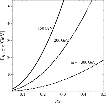
The constraint from 8 TeV LHC data for diphoton searches should be taken into account, since can be sizable in our model. We take the following as the constraint:
| (V.15) |
The ratio of a 13 TeV cross section and an 8 TeV cross section for gluon fusion is estimated as [11]. For the photon fusion process, we write the ratio as . Here is estimated to be [145] but the uncertainty is large, so it can be a larger value [31, 145, 182]. In our analysis, we investigate the constraint using and 4 as reference values.


Finally, we estimate for the cases of , and where we assume the couplings take the same value for all charged scalars for simplicity. Also, the mass of the charged scalar is set to be GeV to enhance loop function inside the diphoton decay width. We show the contours of and in Fig. 9 by solid and dashed lines, respectively, for , and the constraints from diphoton searches at 8 TeV for and are indicated by the purple dashed and the red dotted lines where the region above the lines is excluded. We find that contribution from the photon fusion process is dominant in the parameter region, explaining the diphoton excess. Note here that the contribution from gluon fusion is required to avoid the constraint from an 8 TeV diphoton search for , so we adopt , which is allowed by the constraint of the SM Higgs mixing angle [224, 225, 226, 96]. Then we can obtain fb cross section for all =2 and fb for . We also find that the total decay width is GeV and becomes larger for larger due to contribution from the channel.
Here we comment on collider phenomenology of the boson. The couples to SM particles via - mixing which is induced from kinetic mixing between and gauge fields, . For GeV, the kinetic mixing parameter is limited as experimentally [227, 228]. With this tiny kinetic mixing parameter, we have a very small cross section for production via the Drell-Yan process. Thus, will be dominantly produced through the process without suppression by kinetic mixing. The produced then decays such that , etc. through the mixing effect. From Eq. (V.7), we can derive the production cross section as . Then we obtain fb at the LHC 13 TeV with a reference parameter set , , , TeV, and GeV, which can explain diphoton excess. Thus, the production cross section can be sizable, since , and the LHC experiments can explore the production process with sufficient luminosity. For , the decay width of is roughly , which provides a lifetime of as s for GeV. Then the produced will decay before reaching the detectors at the LHC. We also note that the production cross section for provides a small contribution for , which is preferred by the relic density of DM, since is off-shell.
Before closing this section, let us discuss the consistency of DM relic density calculation with perturbative unitarity constraints on the trilinear scalar couplings, which are given by Eq. (V.4). Note that the VEV of is related to and as in Eq. (II.7). Taking and as in Sec.III, the value of in our scenario is typically 400 to 500 GeV since to 100 GeV to explain the relic density of DM as shown in Figs. 5 and 7. Thus the trilinear coupling should satisfy TeV when we require to satisfy perturbative unitarity safely. Therefore, the and cases have parameter spaces satisfying the condition and explaining the diphoton excess, while the and cases require trilinear coupling larger than the value required by the unitarity condition, in order to explain the diphoton excess. Note that if we lose the perturbative condition as , then the cases of and also have allowed parameter space. However, we need careful analysis to find a parameter space that satisfies perturbative unitarity, which is beyond the scope of this work.
VI Conclusions and discussions
We have proposed a new three-loop induced radiative neutrino model with local dark symmetry, in which the discrepancy of the muon anomalous magnetic moment within the standard model can be resolved by using exotic charged fermions, and both DM candidates (the Majorana fermion and/or scalar) can satisfy the observed thermal relic density without conflict with the results of direct detection searches, considering that the DM pair annihilation into a pair of bosons is supposed to be the dominant process . We have also generalized the hypercharges of isospin doublet fields as well as isospin singlet fields without violating the structure of neutrino masses at the three-loop level. As a result, a lot of electrically charged new fields can be involved in our theory. In this case, such a general value of hypercharge could cause a stability problem; therefore, we have to make them decay into the SM (or DM) appropriately. In order to realize this, we have added some more nonzero charged bosons, and have shown the appropriate decay processes for each value of hypercharge, retaining our model structure for the neutrino masses and mixings. Here such new bosons also play a role in contributing the diphoton excess at 750 GeV that was reported recently by both ATLAS and CMS collaborations.
Then, we have investigated the production of the 750 GeV scalar particle which appears as a linear combination of the SM Higgs and a neutral CP even component of the charged SM singlet scalar. This scalar particle is produced by gluon fusion via mixing with SM Higgs, and also by the photon fusion process. We find that a fb cross section for can be obtained by TeV trilinear coupling for and charged scalar, which is safe from tree level unitarity. The decay width of is GeV due to the contribution from the mode, where a larger gauge coupling would generate a larger width of . Moreover, we have shown that the constraint from a diphoton search at 8 TeV can be satisfied. Thus, we have explained the diphoton excess naturally, depending on the number of hypercharge for new isospin doublet scalar field.
Before closing, we would like to emphasize that the three-loop radiative neutrino mass model presented in this paper is new and has its own value even if the 750 GeV diphoton excess goes away in the future. The three-loop diagrams relevant for the neutrino masses within this model are topologically different from the previous models in the literature, if we trace the dark charge flows in the Feynman diagrams. The model would remain as an interesting and viable model for radiative neutrino masses and also for the muon . As such, it deserves its own investigation at current and future colliders, and in low energy lepton flavor physics.
Acknowledgments
H.O. thanks Shinya Kanemura, Kenji Nishiwaki, Seong Chan Park, Ryoutaro Watanabe and Kei Yagyu for fruitful discussions. This work is supported in part by National Research Foundation of Korea (NRF) Research Grant No. NRF-2015R1A2A1A05001869 (PK), and by the SRC program of NRF Grant No. 20120001176 funded by MEST through the Korea Neutrino Research Center at Seoul National University (P.K., Y.O.).
Appendix
Here we explicitly show the loop functions that appear in the neutrino sector:
| (VI.1) | ||||
| (VI.2) | ||||
| (VI.3) | ||||
| (VI.4) |
with
| (VI.5) | ||||
| (VI.6) | ||||
| (VI.7) | ||||
| (VI.8) | ||||
| (VI.9) | ||||
| (VI.10) |
where and are the masses of and and satisfy and we define , and .
References
- [1] The ATLAS collaboration, ATLAS-CONF-2015-081.
- [2] CMS Collaboration [CMS Collaboration], collisions at 13TeV,” CMS-PAS-EXO-15-004.
- [3] K. Harigaya and Y. Nomura, arXiv:1512.04850 [hep-ph].
- [4] Y. Mambrini, G. Arcadi and A. Djouadi, arXiv:1512.04913 [hep-ph].
- [5] M. Backovic, A. Mariotti and D. Redigolo, arXiv:1512.04917 [hep-ph].
- [6] A. Angelescu, A. Djouadi and G. Moreau, arXiv:1512.04921 [hep-ph].
- [7] Y. Nakai, R. Sato and K. Tobioka, arXiv:1512.04924 [hep-ph].
- [8] S. Knapen, T. Melia, M. Papucci and K. Zurek, arXiv:1512.04928 [hep-ph].
- [9] D. Buttazzo, A. Greljo and D. Marzocca, arXiv:1512.04929 [hep-ph].
- [10] A. Pilaftsis, arXiv:1512.04931 [hep-ph].
- [11] R. Franceschini et al., arXiv:1512.04933 [hep-ph].
- [12] S. Di Chiara, L. Marzola and M. Raidal, arXiv:1512.04939 [hep-ph].
- [13] T. Higaki, K. S. Jeong, N. Kitajima and F. Takahashi, arXiv:1512.05295 [hep-ph].
- [14] S. D. McDermott, P. Meade and H. Ramani, arXiv:1512.05326 [hep-ph].
- [15] J. Ellis, S. A. R. Ellis, J. Quevillon, V. Sanz and T. You, arXiv:1512.05327 [hep-ph].
- [16] M. Low, A. Tesi and L. T. Wang, arXiv:1512.05328 [hep-ph].
- [17] B. Bellazzini, R. Franceschini, F. Sala and J. Serra, arXiv:1512.05330 [hep-ph].
- [18] R. S. Gupta, S. Jager, Y. Kats, G. Perez and E. Stamou, arXiv:1512.05332 [hep-ph].
- [19] C. Petersson and R. Torre, arXiv:1512.05333 [hep-ph].
- [20] E. Molinaro, F. Sannino and N. Vignaroli, arXiv:1512.05334 [hep-ph].
- [21] B. Dutta, Y. Gao, T. Ghosh, I. Gogoladze and T. Li, arXiv:1512.05439 [hep-ph].
- [22] Q. H. Cao, Y. Liu, K. P. Xie, B. Yan and D. M. Zhang, arXiv:1512.05542 [hep-ph].
- [23] S. Matsuzaki and K. Yamawaki, arXiv:1512.05564 [hep-ph].
- [24] A. Kobakhidze, F. Wang, L. Wu, J. M. Yang and M. Zhang, arXiv:1512.05585 [hep-ph].
- [25] R. Martinez, F. Ochoa and C. F. Sierra, arXiv:1512.05617 [hep-ph].
- [26] P. Cox, A. D. Medina, T. S. Ray and A. Spray, arXiv:1512.05618 [hep-ph].
- [27] D. Becirevic, E. Bertuzzo, O. Sumensari and R. Z. Funchal, arXiv:1512.05623 [hep-ph].
- [28] J. M. No, V. Sanz and J. Setford, arXiv:1512.05700 [hep-ph].
- [29] S. V. Demidov and D. S. Gorbunov, arXiv:1512.05723 [hep-ph].
- [30] W. Chao, R. Huo and J. H. Yu, arXiv:1512.05738 [hep-ph].
- [31] S. Fichet, G. von Gersdorff and C. Royon, arXiv:1512.05751 [hep-ph].
- [32] D. Curtin and C. B. Verhaaren, arXiv:1512.05753 [hep-ph].
- [33] L. Bian, N. Chen, D. Liu and J. Shu, arXiv:1512.05759 [hep-ph].
- [34] J. Chakrabortty, A. Choudhury, P. Ghosh, S. Mondal and T. Srivastava, arXiv:1512.05767 [hep-ph].
- [35] A. Ahmed, B. M. Dillon, B. Grzadkowski, J. F. Gunion and Y. Jiang, arXiv:1512.05771 [hep-ph].
- [36] P. Agrawal, J. Fan, B. Heidenreich, M. Reece and M. Strassler, arXiv:1512.05775 [hep-ph].
- [37] C. Csaki, J. Hubisz and J. Terning, arXiv:1512.05776 [hep-ph].
- [38] A. Falkowski, O. Slone and T. Volansky, arXiv:1512.05777 [hep-ph].
- [39] D. Aloni, K. Blum, A. Dery, A. Efrati and Y. Nir, arXiv:1512.05778 [hep-ph].
- [40] Y. Bai, J. Berger and R. Lu, arXiv:1512.05779 [hep-ph].
- [41] E. Gabrielli, K. Kannike, B. Mele, M. Raidal, C. Spethmann and H. Veermae, arXiv:1512.05961 [hep-ph].
- [42] R. Benbrik, C. H. Chen and T. Nomura, arXiv:1512.06028 [hep-ph].
- [43] J. S. Kim, J. Reuter, K. Rolbiecki and R. R. de Austri, arXiv:1512.06083 [hep-ph].
- [44] A. Alves, A. G. Dias and K. Sinha, arXiv:1512.06091 [hep-ph].
- [45] E. Megias, O. Pujolas and M. Quiros, arXiv:1512.06106 [hep-ph].
- [46] L. M. Carpenter, R. Colburn and J. Goodman, arXiv:1512.06107 [hep-ph].
- [47] J. Bernon and C. Smith, arXiv:1512.06113 [hep-ph].
- [48] W. Chao, arXiv:1512.06297 [hep-ph].
- [49] M. T. Arun and P. Saha, arXiv:1512.06335 [hep-ph].
- [50] C. Han, H. M. Lee, M. Park and V. Sanz, arXiv:1512.06376 [hep-ph].
- [51] S. Chang, arXiv:1512.06426 [hep-ph].
- [52] I. Chakraborty and A. Kundu, arXiv:1512.06508 [hep-ph].
- [53] R. Ding, L. Huang, T. Li and B. Zhu, arXiv:1512.06560 [hep-ph].
- [54] H. Han, S. Wang and S. Zheng, arXiv:1512.06562 [hep-ph].
- [55] X. F. Han and L. Wang, arXiv:1512.06587 [hep-ph].
- [56] M. x. Luo, K. Wang, T. Xu, L. Zhang and G. Zhu, arXiv:1512.06670 [hep-ph].
- [57] J. Chang, K. Cheung and C. T. Lu, arXiv:1512.06671 [hep-ph].
- [58] D. Bardhan, D. Bhatia, A. Chakraborty, U. Maitra, S. Raychaudhuri and T. Samui, arXiv:1512.06674 [hep-ph].
- [59] T. F. Feng, X. Q. Li, H. B. Zhang and S. M. Zhao, arXiv:1512.06696 [hep-ph].
- [60] O. Antipin, M. Mojaza and F. Sannino, arXiv:1512.06708 [hep-ph].
- [61] F. Wang, L. Wu, J. M. Yang and M. Zhang, arXiv:1512.06715 [hep-ph].
- [62] J. Cao, C. Han, L. Shang, W. Su, J. M. Yang and Y. Zhang, arXiv:1512.06728 [hep-ph].
- [63] F. P. Huang, C. S. Li, Z. L. Liu and Y. Wang, arXiv:1512.06732 [hep-ph].
- [64] W. Liao and H. q. Zheng, arXiv:1512.06741 [hep-ph].
- [65] J. J. Heckman, arXiv:1512.06773 [hep-ph].
- [66] M. Dhuria and G. Goswami, arXiv:1512.06782 [hep-ph].
- [67] X. J. Bi, Q. F. Xiang, P. F. Yin and Z. H. Yu, arXiv:1512.06787 [hep-ph].
- [68] J. S. Kim, K. Rolbiecki and R. R. de Austri, arXiv:1512.06797 [hep-ph].
- [69] L. Berthier, J. M. Cline, W. Shepherd and M. Trott, arXiv:1512.06799 [hep-ph].
- [70] W. S. Cho, D. Kim, K. Kong, S. H. Lim, K. T. Matchev, J. C. Park and M. Park, arXiv:1512.06824 [hep-ph].
- [71] J. M. Cline and Z. Liu, arXiv:1512.06827 [hep-ph].
- [72] M. Bauer and M. Neubert, arXiv:1512.06828 [hep-ph].
- [73] M. Chala, M. Duerr, F. Kahlhoefer and K. Schmidt-Hoberg, arXiv:1512.06833 [hep-ph].
- [74] D. Barducci, A. Goudelis, S. Kulkarni and D. Sengupta, arXiv:1512.06842 [hep-ph].
- [75] S. M. Boucenna, S. Morisi and A. Vicente, arXiv:1512.06878 [hep-ph].
- [76] C. W. Murphy, arXiv:1512.06976 [hep-ph].
- [77] A. E. C. Hernandez and I. Nisandzic, arXiv:1512.07165 [hep-ph].
- [78] U. K. Dey, S. Mohanty and G. Tomar, arXiv:1512.07212 [hep-ph].
- [79] G. M. Pelaggi, A. Strumia and E. Vigiani, arXiv:1512.07225 [hep-ph].
- [80] J. de Blas, J. Santiago and R. Vega-Morales, arXiv:1512.07229 [hep-ph].
- [81] A. Belyaev, G. Cacciapaglia, H. Cai, T. Flacke, A. Parolini and H. Serodio, arXiv:1512.07242 [hep-ph].
- [82] P. S. B. Dev and D. Teresi, arXiv:1512.07243 [hep-ph].
- [83] W. C. Huang, Y. L. S. Tsai and T. C. Yuan, arXiv:1512.07268 [hep-ph].
- [84] S. Moretti and K. Yagyu, arXiv:1512.07462 [hep-ph].
- [85] K. M. Patel and P. Sharma, arXiv:1512.07468 [hep-ph].
- [86] M. Badziak, arXiv:1512.07497 [hep-ph].
- [87] S. Chakraborty, A. Chakraborty and S. Raychaudhuri, arXiv:1512.07527 [hep-ph].
- [88] Q. H. Cao, S. L. Chen and P. H. Gu, arXiv:1512.07541 [hep-ph].
- [89] W. Altmannshofer, J. Galloway, S. Gori, A. L. Kagan, A. Martin and J. Zupan, arXiv:1512.07616 [hep-ph].
- [90] M. Cvetic, J. Halverson and P. Langacker, arXiv:1512.07622 [hep-ph].
- [91] J. Gu and Z. Liu, arXiv:1512.07624 [hep-ph].
- [92] B. C. Allanach, P. S. B. Dev, S. A. Renner and K. Sakurai, arXiv:1512.07645 [hep-ph].
- [93] H. Davoudiasl and C. Zhang, arXiv:1512.07672 [hep-ph].
- [94] N. Craig, P. Draper, C. Kilic and S. Thomas, arXiv:1512.07733 [hep-ph].
- [95] K. Das and S. K. Rai, arXiv:1512.07789 [hep-ph].
- [96] K. Cheung, P. Ko, J. S. Lee, J. Park and P. Y. Tseng, arXiv:1512.07853 [hep-ph].
- [97] J. Liu, X. P. Wang and W. Xue, arXiv:1512.07885 [hep-ph].
- [98] J. Zhang and S. Zhou, arXiv:1512.07889 [hep-ph].
- [99] J. A. Casas, J. R. Espinosa and J. M. Moreno, arXiv:1512.07895 [hep-ph].
- [100] L. J. Hall, K. Harigaya and Y. Nomura, arXiv:1512.07904 [hep-ph].
- [101] H. Han, S. Wang and S. Zheng, arXiv:1512.07992 [hep-ph].
- [102] J. C. Park and S. C. Park, arXiv:1512.08117 [hep-ph].
- [103] A. Salvio and A. Mazumdar, arXiv:1512.08184 [hep-ph].
- [104] D. Chway, R. Dermisek, T. H. Jung and H. D. Kim, arXiv:1512.08221 [hep-ph].
- [105] G. Li, Y. n. Mao, Y. L. Tang, C. Zhang, Y. Zhou and S. h. Zhu, arXiv:1512.08255 [hep-ph].
- [106] M. Son and A. Urbano, arXiv:1512.08307 [hep-ph].
- [107] Y. L. Tang and S. h. Zhu, arXiv:1512.08323 [hep-ph].
- [108] H. An, C. Cheung and Y. Zhang, arXiv:1512.08378 [hep-ph].
- [109] J. Cao, F. Wang and Y. Zhang, arXiv:1512.08392 [hep-ph].
- [110] F. Wang, W. Wang, L. Wu, J. M. Yang and M. Zhang, arXiv:1512.08434 [hep-ph].
- [111] C. Cai, Z. H. Yu and H. H. Zhang, arXiv:1512.08440 [hep-ph].
- [112] Q. H. Cao, Y. Liu, K. P. Xie, B. Yan and D. M. Zhang, arXiv:1512.08441 [hep-ph].
- [113] J. E. Kim, arXiv:1512.08467 [hep-ph].
- [114] J. Gao, H. Zhang and H. X. Zhu, arXiv:1512.08478 [hep-ph].
- [115] W. Chao, arXiv:1512.08484 [hep-ph].
- [116] X. J. Bi et al., arXiv:1512.08497 [hep-ph].
- [117] F. Goertz, J. F. Kamenik, A. Katz and M. Nardecchia, arXiv:1512.08500 [hep-ph].
- [118] L. A. Anchordoqui, I. Antoniadis, H. Goldberg, X. Huang, D. Lust and T. R. Taylor, arXiv:1512.08502 [hep-ph].
- [119] P. S. B. Dev, R. N. Mohapatra and Y. Zhang, arXiv:1512.08507 [hep-ph].
- [120] N. Bizot, S. Davidson, M. Frigerio and J.-L. Kneur, arXiv:1512.08508 [hep-ph].
- [121] L. E. Ibanez and V. Martin-Lozano, arXiv:1512.08777 [hep-ph].
- [122] C. W. Chiang, M. Ibe and T. T. Yanagida, arXiv:1512.08895 [hep-ph].
- [123] S. K. Kang and J. Song, arXiv:1512.08963 [hep-ph].
- [124] Y. Hamada, T. Noumi, S. Sun and G. Shiu, arXiv:1512.08984 [hep-ph].
- [125] X. J. Huang, W. H. Zhang and Y. F. Zhou, arXiv:1512.08992 [hep-ph].
- [126] S. Kanemura, K. Nishiwaki, H. Okada, Y. Orikasa, S. C. Park and R. Watanabe, arXiv:1512.09048 [hep-ph].
- [127] S. Kanemura, N. Machida, S. Odori and T. Shindou, arXiv:1512.09053 [hep-ph].
- [128] I. Low and J. Lykken, arXiv:1512.09089 [hep-ph].
- [129] A. E. C. Hernandez, arXiv:1512.09092 [hep-ph].
- [130] Y. Jiang, Y. Y. Li and T. Liu, arXiv:1512.09127 [hep-ph].
- [131] K. Kaneta, S. Kang and H. S. Lee, arXiv:1512.09129 [hep-ph].
- [132] L. Marzola, A. Racioppi, M. Raidal, F. R. Urban and H. Veermae, arXiv:1512.09136 [hep-ph].
- [133] E. Ma, arXiv:1512.09159 [hep-ph].
- [134] A. Dasgupta, M. Mitra and D. Borah, arXiv:1512.09202 [hep-ph].
- [135] S. Jung, J. Song and Y. W. Yoon, arXiv:1601.00006 [hep-ph].
- [136] C. T. Potter, arXiv:1601.00240 [hep-ph].
- [137] E. Palti, arXiv:1601.00285 [hep-ph].
- [138] T. Nomura and H. Okada, arXiv:1601.00386 [hep-ph].
- [139] X. F. Han, L. Wang, L. Wu, J. M. Yang and M. Zhang, arXiv:1601.00534 [hep-ph].
- [140] P. Ko, Y. Omura and C. Yu, arXiv:1601.00586 [hep-ph].
- [141] K. Ghorbani and H. Ghorbani, arXiv:1601.00602 [hep-ph].
- [142] D. Palle, arXiv:1601.00618 [physics.gen-ph].
- [143] U. Danielsson, R. Enberg, G. Ingelman and T. Mandal, arXiv:1601.00624 [hep-ph].
- [144] W. Chao, arXiv:1601.00633 [hep-ph].
- [145] C. Csaki, J. Hubisz, S. Lombardo and J. Terning, arXiv:1601.00638 [hep-ph].
- [146] A. Karozas, S. F. King, G. K. Leontaris and A. K. Meadowcroft, arXiv:1601.00640 [hep-ph].
- [147] A. E. C. Hernandez, I. d. M. Varzielas and E. Schumacher, arXiv:1601.00661 [hep-ph].
- [148] T. Modak, S. Sadhukhan and R. Srivastava, arXiv:1601.00836 [hep-ph].
- [149] B. Dutta, Y. Gao, T. Ghosh, I. Gogoladze, T. Li, Q. Shafi and J. W. Walker, arXiv:1601.00866 [hep-ph].
- [150] F. F. Deppisch, C. Hati, S. Patra, P. Pritimita and U. Sarkar, arXiv:1601.00952 [hep-ph].
- [151] H. Ito, T. Moroi and Y. Takaesu, arXiv:1601.01144 [hep-ph].
- [152] H. Zhang, arXiv:1601.01355 [hep-ph].
- [153] A. Berlin, arXiv:1601.01381 [hep-ph].
- [154] S. Bhattacharya, S. Patra, N. Sahoo and N. Sahu, arXiv:1601.01569 [hep-ph].
- [155] F. D’Eramo, J. de Vries and P. Panci, arXiv:1601.01571 [hep-ph].
- [156] I. Sahin, arXiv:1601.01676 [hep-ph].
- [157] S. Fichet, G. von Gersdorff and C. Royon, arXiv:1601.01712 [hep-ph].
- [158] D. Borah, S. Patra and S. Sahoo, arXiv:1601.01828 [hep-ph].
- [159] D. Stolarski and R. Vega-Morales, arXiv:1601.02004 [hep-ph].
- [160] M. Fabbrichesi and A. Urbano, arXiv:1601.02447 [hep-ph].
- [161] C. Hati, arXiv:1601.02457 [hep-ph].
- [162] P. Ko and T. Nomura, arXiv:1601.02490 [hep-ph].
- [163] J. Cao, L. Shang, W. Su, Y. Zhang and J. Zhu, arXiv:1601.02570 [hep-ph].
- [164] J. H. Yu, arXiv:1601.02609 [hep-ph].
- [165] R. Ding, Z. L. Han, Y. Liao and X. D. Ma, arXiv:1601.02714 [hep-ph].
- [166] S. Alexander and L. Smolin, arXiv:1601.03091 [hep-ph].
- [167] J. H. Davis, M. Fairbairn, J. Heal and P. Tunney, arXiv:1601.03153 [hep-ph].
- [168] I. Dorsner, S. Fajfer and N. Kosnik, arXiv:1601.03267 [hep-ph].
- [169] A. E. Faraggi and J. Rizos, arXiv:1601.03604 [hep-ph].
- [170] A. Djouadi, J. Ellis, R. Godbole and J. Quevillon, arXiv:1601.03696 [hep-ph].
- [171] A. Ghoshal, arXiv:1601.04291 [hep-ph].
- [172] T. Nomura and H. Okada, arXiv:1601.04516 [hep-ph].
- [173] W. Chao, arXiv:1601.04678 [hep-ph].
- [174] X. F. Han, L. Wang and J. M. Yang, arXiv:1601.04954 [hep-ph].
- [175] H. Okada and K. Yagyu, arXiv:1601.05038 [hep-ph].
- [176] D. B. Franzosi and M. T. Frandsen, arXiv:1601.05357 [hep-ph].
- [177] A. Martini, K. Mawatari and D. Sengupta, arXiv:1601.05729 [hep-ph].
- [178] Q. H. Cao, Y. Q. Gong, X. Wang, B. Yan and L. L. Yang, arXiv:1601.06374 [hep-ph].
- [179] C. W. Chiang and A. L. Kuo, arXiv:1601.06394 [hep-ph]; C. W. Chiang, A. L. Kuo and T. Yamada, JHEP 1601, 120 (2016) [arXiv:1511.00865 [hep-ph]].
- [180] U. Aydemir and T. Mandal, arXiv:1601.06761 [hep-ph].
- [181] S. Abel and V. V. Khoze, arXiv:1601.07167 [hep-ph].
- [182] L. A. Harland-Lang, V. A. Khoze and M. G. Ryskin, arXiv:1601.07187 [hep-ph].
- [183] S. F. King and R. Nevzorov, arXiv:1601.07242 [hep-ph].
- [184] J. Kawamura and Y. Omura, arXiv:1601.07396 [hep-ph].
- [185] B. J. Kavanagh, arXiv:1601.07330 [hep-ph].
- [186] T. Nomura and H. Okada, arXiv:1601.07339 [hep-ph].
- [187] C. Q. Geng and D. Huang, arXiv:1601.07385 [hep-ph].
- [188] E. Bertuzzo, P. A. N. Machado and M. Taoso, arXiv:1601.07508 [hep-ph].
- [189] I. Ben-Dayan and R. Brustein, arXiv:1601.07564 [hep-ph].
- [190] N. D. Barrie, A. Kobakhidze, M. Talia and L. Wu, doi:10.1016/j.physletb.2016.02.010 arXiv:1602.00475 [hep-ph].
- [191] L. Aparicio, A. Azatov, E. Hardy and A. Romanino, arXiv:1602.00949 [hep-ph].
- [192] R. Ding, Y. Fan, L. Huang, C. Li, T. Li, S. Raza and B. Zhu, arXiv:1602.00977 [hep-ph].
- [193] T. Li, J. A. Maxin, V. E. Mayes and D. V. Nanopoulos, arXiv:1602.01377 [hep-ph].
- [194] A. Salvio, F. Staub, A. Strumia and A. Urbano, arXiv:1602.01460 [hep-ph].
- [195] S. F. Ge, H. J. He, J. Ren and Z. Z. Xianyu, arXiv:1602.01801 [hep-ph].
- [196] S. B. Giddings and H. Zhang, arXiv:1602.02793 [hep-ph].
- [197] U. Ellwanger and C. Hugonie, arXiv:1602.03344 [hep-ph].
- [198] C. Arbelaez, A. E. C. Hernandez, S. Kovalenko and I. Schmidt, arXiv:1602.03607 [hep-ph].
- [199] K. J. Bae, M. Endo, K. Hamaguchi and T. Moroi, arXiv:1602.03653 [hep-ph].
- [200] C. Gross, O. Lebedev and J. M. No, arXiv:1602.03877 [hep-ph].
- [201] C. Han, T. T. Yanagida and N. Yokozaki, arXiv:1602.04204 [hep-ph].
- [202] Y. Hamada, H. Kawai, K. Kawana and K. Tsumura, arXiv:1602.04170 [hep-ph].
- [203] B. Dasgupta, J. Kopp and P. Schwaller, arXiv:1602.04692 [hep-ph].
- [204] F. Goertz, A. Katz, M. Son and A. Urbano, arXiv:1602.04801 [hep-ph].
- [205] Y. J. Zhang, B. B. Zhou and J. J. Sun, arXiv:1602.05539 [hep-ph].
- [206] F. Staub et al., arXiv:1602.05581 [hep-ph].
- [207] S. Baek and J. h. Park, arXiv:1602.05588 [hep-ph].
- [208] M. Cvetic, J. Halverson and P. Langacker, arXiv:1602.06257 [hep-ph].
- [209] D. S. Akerib et al. [LUX Collaboration], Phys. Rev. Lett. 112, 091303 (2014) [arXiv:1310.8214 [astro-ph.CO]].
- [210] S. Baek, P. Ko and W. I. Park, Phys. Lett. B 747, 255 (2015) [arXiv:1407.6588 [hep-ph]].
- [211] H. Okada and K. Yagyu, Phys. Rev. D 93, no. 1, 013004 (2016) [arXiv:1508.01046 [hep-ph]].
- [212] K.A. Olive et al. (Particle Data Group), Chin. Phys. C, 38, 090001 (2014).
- [213] L. M. Krauss, S. Nasri and M. Trodden, Phys. Rev. D 67, 085002 (2003) [hep-ph/0210389].
- [214] M. Aoki, S. Kanemura and O. Seto, Phys. Rev. Lett. 102, 051805 (2009) [arXiv:0807.0361 [hep-ph]].
- [215] M. Gustafsson, J. M. No and M. A. Rivera, Phys. Rev. Lett. 110, no. 21, 211802 (2013) Erratum: [Phys. Rev. Lett. 112, no. 25, 259902 (2014)] [arXiv:1212.4806 [hep-ph]].
- [216] F. Jegerlehner and A. Nyffeler, Phys. Rept. 477, 1 (2009) [arXiv:0902.3360 [hep-ph]].
- [217] M. Benayoun, P. David, L. Delbuono and F. Jegerlehner, Eur. Phys. J. C 72, 1848 (2012) [arXiv:1106.1315 [hep-ph]].
- [218] J. Adam et al. [MEG Collaboration], Phys. Rev. Lett. 110, 201801 (2013) [arXiv:1303.0754 [hep-ex]].
- [219] P. A. R. Ade et al. [Planck Collaboration], Astron. Astrophys. (2014) [arXiv:1303.5076 [astro-ph.CO]].
- [220] P. Gondolo and G. Gelmini, Nucl. Phys. B 360, 145 (1991).
- [221] A. Djouadi, L. Maiani, G. Moreau, A. Polosa, J. Quevillon and V. Riquer, Eur. Phys. J. C 73, 2650 (2013) [arXiv:1307.5205 [hep-ph]].
- [222] V. Khachatryan et al. [CMS Collaboration], JHEP 1410, 160 (2014) [arXiv:1408.3316 [hep-ex]].
- [223] J. F. Gunion, H. E. Haber, G. L. Kane and S. Dawson, Front. Phys. 80, 1 (2000).
- [224] The numerical analyses on the Higgs decays are performed using the program HDECAY: A. Djouadi, J. Kalinowski and M. Spira, Comput. Phys. Commun. 108 (1998) 56; A. Djouadi, M. Muhlleitner and M. Spira, Acta. Phys. Polon. B38 (2007) 635.
- [225] S. Choi, S. Jung and P. Ko, JHEP 1310, 225 (2013) [arXiv:1307.3948 [hep-ph]].
- [226] K. Cheung, P. Ko, J. S. Lee and P. Y. Tseng, JHEP 1510, 057 (2015) [arXiv:1507.06158 [hep-ph]].
- [227] S. Andreas, C. Niebuhr and A. Ringwald, Phys. Rev. D 86 (2012) 095019 [arXiv:1209.6083 [hep-ph]].
- [228] J. Jaeckel, M. Jankowiak and M. Spannowsky, Phys. Dark Univ. 2, 111 (2013) [arXiv:1212.3620 [hep-ph]].