Cosmological models in Weyl geometrical scalar-tensor theory
Abstract
We investigate cosmological models in a recently proposed geometrical theory of gravity, in which the scalar field appears as part of the space-time geometry. We extend the previous theory to include a scalar potential in the action. We solve the vacuum field equations for different choices of the scalar potential and give a detailed analysis of the solutions. We show that in some cases a cosmological scenario is found that seems to suggest the appearance of a geometric phase transition. We build a toy model, in which the accelerated expansion of the early universe is driven by pure geometry.
pacs
04.20.Jb, 11.10.kk, 98.80.CqI Introduction
Scalar-tensor theories have attracted the attention of cosmologists since a seminal work by Jordan was published in the fifties [1]. However, the great impetus to investigate these kinds of theories came from Brans-Dicke theory, which is considered by many as the most popular and simplest alternative theory of gravity [2]. In the last three decades, interest in scalar-tensor theory has increased, mainly motivated by modern Kaluza-Klein theory, string theory, inflationary models, and other recent proposals. As is well known, scalar-tensor theories in general do not assign an intrinsic geometric character to the scalar field. Nor does this field describe matter in the usual sense. In the particular case of Brans-Dicke theory, its role is to account for possible variations of Newton’s gravitational constant, since the latter, according to Mach ideas, would depend on the mass of the universe [3]. However, there have been some attempts to construct a scalar-tensor theory of gravitation in which the scalar field is an essential part of the space-time geometry [4]. In all these cases, one looks for a geometrical framework that contains a scalar field as a way of adding a new degree of freedom to the corresponding gravity theory.
In the present article, we consider a scalar-tensor theory of gravity, in which the scalar field does play a geometric role. The mechanism for inserting the scalar field in the space-time geometry is inspired by Weyl’s generalization of Riemannian geometry, in the very special case when the gauge field corresponds to an exact 1-form [5]. The space-time structure that results from this kind of geometry is known in the literature as a Weyl integrable space-time (WIST) [6]. The first approach to a scalar-tensor theory set in a WIST was proposed by Novello et al, and consists of a direct extension of general relativity by including in the Einstein-Hilbert action a term corresponding to a massless scalar field, the latter being interpreted as a geometrical field in the sense of Weyl geometry [7]. A more recent geometrical approach to scalar-tensor theory (GST) starts by considering the action of Brans-Dicke theory and introduces the space-time geometry from first principles, that is, by applying the Palatini formalism, which then leads to a Weyl integrable geometry [8]. Although the original version of GST theory does not include a scalar potential in the action, the inclusion of such term is rather natural and does not alter the geometrical aspects of the theory. Thus, in this paper we consider a slightly modified version of original proposal by adding a scalar potential. Certainly, the main motivation for this modification lies in the fact that in modern cosmology scalar potentials are an important ingredient of inflationary models, quintessence, and other theories.
This article is organized as follows. In Section 2, we give a brief review of the geometrical scalar-tensor theory and consider its extension to include a scalar potential. In Section 3, we discuss the application of the geometric scalar-tensor theory to some cosmological scenarios, in which matter can be neglected as the potential energy of the scalar field is the dominant contribution. In Section 4, we construct a very simple cosmological model, a sort of “toy model”, in which a phase of accelerated expansion of the universe is driven by pure geometry. We conclude in Section V with some remarks.
II The Weyl geometrical scalar-tensor theory
The Weyl geometrical scalar-tensor theory starts with the action given by
| (1) |
where , is a scalar field, is a function of , represents the scalar field potential, and indicates the part of the action depending on the matter fields, here generically denoted by 11 1 Note that this action is a simple extension of the action considered in [8]. Let us recall that is regarded as a purely geometrical field, whose meaning becomes clear only after a Palatini variation of the action above is carried out. Indeed, it is known that the variation of (1) with respect to the affine connection leads to [8]
| (2) |
an equation that expresses the so-called Weyl compatibility condition between the metric and the connection (also called Weyl nonmetricity condition)22 2 Throughout the paper we shall use the following convention: Whenever the symbol appears in the expression it denotes Otherwise denotes the metric tensor. We shall also consider the Ricci tensor as being given in terms of the affine connection coefficients via the definition of the curvature tensor.. This is the geometric condition that characterizes the space-time manifold as a Weyl integrable space-time [6]. By performing the Palatini variation with respect to the metric and the scalar field we obtain the following set of field equations:
| (3) |
| (4) |
where the symbol denotes the d’Alembertian operator calculated with respect to the Weyl connection, , and represents the Weyl invariant energy-momentum tensor of the matter fields as defined in [8].
II.1 The field equations in the Riemann frame
As is well known, the Weyl condition (2) does not change when we perform the following transformations in and :
| (5) |
| (6) |
where is an arbitrary scalar function defined on the manifold space-time . These transformations are known, in the literature, as Weyl transformations. The set consisting of a differentiable manifold endowed with a metric and a Weyl scalar field will be called a Weyl frame. We now note that if we set in (6), we get . In this case, when the Weyl scalar field vanishes, the set is referred to as the Riemann frame.
It is sometimes convenient to recast the action (1) and the above field equations in the Riemann frame. It is not difficult to verify that in this frame (1) is transformed into the action
| (7) |
whereas the field equations (3) and (4) are given, respectively, by
| (8) |
| (9) |
where both the Einstein tensor and the operator are calculated with the Levi-Civita connection given in terms of the metric .
III Applications to cosmology
Typical gravitational problems, such as the field generated by a spherically symmetric matter distribution, or the existence of naked singularities and wormholes as geometric phenomena, have already been studied in the context of Weyl geometrical scalar-tensor theory [8]. In this work, we would like to consider some cosmological models arising from different choices of the scalar potential. For convenience, we shall work in the Riemann frame, although due to frame invariance all physical results obtained will be valid in any Weyl frame [8]. Let us point out that the technique of frame transformations to investigate cosmological models with non-minimally coupled scalar fields is not new, and has been used recently [9].
As we have already mentioned, scalar fields have been extensively used in cosmology, mainly motivated by inflationary models, but also as a possible way to account for dark matter and quintessence models of dark energy [10, 11]. In inflationary cosmology, the scalar field (the inflaton) is responsible for the negative pressure needed to expand the universe [12]. Nevertheless, up to now the nature of this scalar field is not known. On the other hand, since the apperance of inflationary cosmology in the 1980’s different models have been proposed, in which the presence of a scalar potential is considered [13]. The simplest of these requires a monomial potential. Despite the fact that the latest observational results do not favour a potential of the type [14], a massive scalar field has been considered by many authors with great interest [15]. In the following sections, we shall consider some simple models for different types of in the context of the Weyl geometrical scalar-tensor theory. In almost cases we shall add the cosmological constant . Throughout our discussion, we shall always take the point of view that the scalar field has an essentially geometric origin. This is because it is always possible to interpret the scalar field as a geometric field by going to the Weyl frame [8].
Let us now start by considering a homogeneous, spatially flat, and isotropic model, whose line element is written as
| (10) |
where denotes the scale factor. Let us also restrict ourselves to the vacuum case and, as in Brans-Dicke theory, let us for simplicity set . Thus, the field equations (8) reduce to
| (11) |
| (12) |
while (9) gives
| (13) |
Expressing the above equations in terms of the expansion parameter , and defining , it is easy to verify, after simple calculations, that we are left with the following equations 33 3 Because the connection is frame-invariant, then the expansion parameter is also invariant. Indeed, by definition , where denotes the 4-velocity field of the fundamental observers. Clearly, in the Riemannian frame the metric takes the form , which is, as we know, invariant. On the other hand, is assumed to be given by (10).:
| (14) |
| (15) |
| (16) |
In the next subsections we shall consider four distinct cases, each one corresponding to a specific choice of the scalar potential .
III.1 The Cosmological Constant
We shall start our analysis with the choice . Clearly, this will lead us, in the Riemann frame, to the case of a massless scalar field minimally coupled to gravity in the presence of a cosmological constant and a free parameter . It is not difficult to check that, for , the field equations (11), (12) and (13) admit the following solutions:
| (17) |
where is a constant of integration. These are, in fact, the simplest of all solutions of the above field equations. The solution corresponds to the well-known de Sitter (anti-de Sitter) universe, a maximally symmetric vacuum solution of Einstein’s field equations with a cosmological constant.
For and , we have two solutions:
| (18) |
| (19) |
These represent a non-singular bouncing universe which bears some similarity to recently proposed models in scalar-tensor theories [16]. On the other hand, if and the solutions are
| (20) |
| (21) |
In this case, we have a model that describes a cyclic universe, which undergoes an eternal series of oscillations, each beginning with a big bang and ending with a big crunch, and in each cycle a period of expansion is followed by a contraction. Let us just remark here that cyclic universes have been favoured by many recent proposals [17]. In particular, cyclic models have also been predicted by loop quantum cosmology through a mechanism by which the contracting and expanding cosmological branches are connected by a “quantum bridge” [18].
Finally, if both and are positive, the solutions will be given by
| (22) |
| (23) |
These solutions are singular at and describe an expanding and accelerating universe which tends to a de Sitter universe when
A nice picture of the time evolution of the above models is given by the phase portraits of the dynamical system corresponding to the field equations, since these portraits may provide an insight on the dynamical behaviour of the solutions. In the next section, we shall give a qualitative analysis of the solutions obtained.
III.2 Phase portrait of the solutions when
In this case, it is easy to verify that the field equations (11)-(12) and (13) reduce to
| (24) |
| (25) |
| (26) |
As we can see, the above equations constitute an autonomous planar dynamical system, with (24) representing an algebraic constraint in the phase space [19].


In order to draw the phase portrait, let us first determine the critical (or equilibrium) points of the system, that is, the points in the phase plane at which the right side of (25) and (26) vanishes. There are four equilibrium points, but only two of them satisfy the constraint equation (24), and these correspond to special solutions, presenting the simplest kind of behaviour. It is not difficult to see that we have equilibrium points only if 44 4 Clearly, the case when and are both negative is not allowed because of (24).. These are and , which lie on the axis and correspond, respectively, to the solutions (17), i.e. , the de Sitter and anti-de Sitter solutions found in the previous section. The solutions for and , obtained above, lie in the ellipse (depicted in bold), which is the only curve in the phase plane satisfying the constraint (24) (see Fig. 1a). The solutions given by the equations (18) and (19) are represented in the diagram as the trajectories starting at and ending at , in the anticlockwise and clockwise sense , respectively. It is interesting to note that the solution corresponding to the point is stable with respect to small perturbations in the phase plane, while has a unstable character. The existence of this kind of stability (instability) pattern associated to the two critical points seems to lead to an interesting behaviour as far as the space-time geometry of these models is concerned. Consider, for instance, the solution represented by the equilibrium point , which, as we know, corresponds to a contracting de Sitter space-time, with a constant scalar field. From the point of view of the Weyl frame , this means that the space-time geometry is Riemannian. Now, let us look at how the space-time geometry evolves when this universe is slightly perturbed. Clearly, the time evolution is either determined by or . Initially, when , these universes are in an purely Riemannian regime as the scalar field is nearly constant. This situation will change as soon as the scalar field ceases to be a constant and gradually starts to depend on time. Then the universe enters a new regime, in which space-time is characterized by a Weyl integrable geometry. One is tempted to say that we have here a kind of geometrical phase transition, since we go from a purely Riemannian geometry to a Weyl integrable geometry. Finally, as , since and both approach the equilibrium point , the universe returns to its initial Riemannian regime, undergoing another geometrical transition, this time from a Weyl geometry to a purely Riemannian de Sitter space-time, represented in the phase portrait by the equilibrium point .
The phase diagram corresponding to the solutions for and , namely, (20) and (21), are depicted as bold lines in Fig. 1b. As the diagram clearly shows, we have two singular universes which start with a big bang, undergo an era of expansion, and finally collapse to a big crunch. Interpreting this picture in the Weyl frame, we see that because the time derivative of the scalar field does not vanish no geometrical phase transition takes place in this case.
Finally, when both and are positive, the phase portrait of the solutions is shown in Fig. 1c. In this case, as regards the solutions given by equations (22) and (23), the critical point behaves as an attractor, while acts as a repellor. In the first situation, we have singular expanding Weyl space-times evolving towards a Riemannian de Sitter universe, while in the second, small perturbations cause a Riemannian anti-de Sitter universe start to collapsing into a big crunch.
To conclude this section, let us, just for the sake of completeness, examine the degenerate case when . In this case, the equations (11), (12) and (13) become
| (27) |
| (28) |
| (29) |
We first note that in order to obtain real solutions we must restrict the parameter to be positive 55 5 The case is trivial, corresponding to Minkowski space-time.. We also note that the conics that appeared in the former phase diagrams, representing the constraint of the dynamical system, now simply degenerate into the pair of straight lines (see Fig. 1d). The equations above are easily integrated and give the following solutions:
| (30) |
| (31) |
We now have only one critical point, which lies at the origin , and this clearly corresponds to Minkowski space-time. For the two solutions given by (30) and (31) start with a big bang and approach as . On the other hand, for we have two other solutions which comes from when , and then collapses to a singular space-time as .
Finally, it should be remarked here that when , the action (7) includes a phantom field. It is known that in this case we have violation of the null energy condition [20]. (It is important to note that the case of constant potential and , has been investigated in a different context (mainly inspired by string field theories) in [21].
Let us now briefly consider other types of scalar potentials.
III.3 Potential of a massive scalar field
In this section, we shall briefly consider a potential of the type In the Riemann frame, this type of potential, which corresponds to the case of a massive scalar field plus a cosmological constant is easily found in the literature of inflationary models, and leads to several different cosmological regimes [24].
By applying a known simple mathematical procedure (first-order formalism) to the field equations (11)-(13) we obtain the following solution [25]
| (32) |
| (33) |
where
| (34) |
and , and are constants of integration.
The field equations for this potential may be put in the form
| (35) |
| (36) |
| (37) |
In the above equations, we can use (35) to eliminate by writing , and thus arrive at the following dynamical system, defined only in terms of the variables and :
| (38) |
| (39) |
Actually, we have two dynamical systems according to whether we take or in (39). The phase portrait of the solutions is displayed below.


Let us now make some comments on the behaviour of the solutions. The critical points are given by and , and, although they are solutions of the dynamical system defined by (38) and (39), they do not represent a solution of the complete set of field equations for . The physical solutions (32) and (33) correspond to the isoclines , and are represented by the two bold straight lines in the diagrams (see Fig. 2, above). It is to be noted that these solutions are continuous with respect to the time parameter , and that, as time goes by, they pass from one diagram to the other diagram continuously. Clearly, the two solutions describe non-singular universes that undergo a contraction era followed by a expanding period, depending on the sign we ascribe to the constant . It also should be noted that, as can be seen from (39), in the (shaded) elliptic region bounded by the curve the dynamical system is not defined. Fig. 2 shows the phase portrait for and , satisfying the condition (34). Let us mention here that models with quadratic potential, appearing in a different context, have been previously considered in which the phase portraits corresponding to the field equations are also discussed [22].
III.4 Exponential scalar potential
Some well-known inflationary models assume that the evolution of the universe during inflation is driven by a scalar field generated by an exponential potential of the form
| (40) |
with and being constants [23]. It is not difficult to verify that, in this case, the field equations (11), (12) and (13) have the following solutions:
| (41) |
| (42) |
Let us remark that these solutions are in agreement with the already known result that exponential potentials generate power-law inflation. (Note that the possible values of the free parameter are restricted to the intervals and .) On the other hand, the expansion parameter of the model is given by
| (43) |
To get a clearer picture of the behaviour of the solutions let us examine the dynamical system obtained from the field equations. It is not difficult to verify that from the set of equations (14), (15), (16) reduces to
| (44) |
| (45) |
| (46) |
With the help of (44) the equations (45) and (46) may be written as
| (47) |
| (48) |
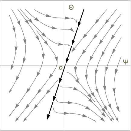

The phase portrait of this dynamical system is displayed in Fig. 3, where the solutions given by (41) and (42), lie on the straight line , passing through the origin , which is the only equilibrium point of the system, and corresponds to Minkowski space-time. In Fig. 3a, we have depicted the solutions for , which represent an expanding model singular, approaching Minkowski space-time as , and a collapsing model starting from Minkowski space-time at evolving towards a singularity.
Quartic potential
We next consider the quadratic potential
| (49) |
where and are positive constants. This particular kind of effective quartic potential has been considered in inflationary scenarios mainly inspired in the idea that it is the Higgs boson that plays the role of the inflaton field [26].
We can easily show that the cosmological equations (11), (12) and (13) admit the following solution:
| (50) |
| (51) |
with , being constants of integration, , and the condition must be satisfied. The expansion factor gives
| (52) |
Clearly, these correspond to non-singular universes undergoing expansion or contraction, depending on the value assumed by the constants.
If we wish to treat the field equations for this potential as a dynamical system, we write them in the form
| (53) |
| (54) |
| (55) |
As in the case of the massive scalar field, the constraint equation (53) can be used to eliminate the variable from the dynamical equations. This procedure will lead us to four distinct dynamical systems. These are given by the following equations:
| (56) |
| (57) |
The first pair of signs in the right-hand side of (57) defines two dynamical systems, corresponding to the two possibles signs of . The other two dynamical systems arise when the second and third pairs of plus or minus signs are fixed simultaneously, according to whether or . The phase portraits of these four dynamical systems (56)-(57) are depicted in Figure 4, below.


As to the critical points, it is not difficult to verify that the origin is an equilibrium point of the four dynamical systems (56)-(57), which corresponds to the trivial case of Minkowski space-time with a constant scalar field (see Eq. (53)). On the other hand, the two dynamical systems for which have two additional critical points: . These represent solutions of the field equations, corresponding to an expanding or a contracting de Sitter universe with a null scalar field.
A comment on the domain of the phase plane where the dynamical systems are defined is now in order. Clearly, the square roots in (56)-(57) restrict the possible values of the dynamical variables. In all cases, the inequality must be satisfied, while in two of them (Fig. 4b and Fig. 4d) we have an additional restriction imposed by .
It is not difficult to verify that the analytic solutions (50)-(51) lie on the parabola , where we are considering the case in which the constants and have the same sign. As an example, let us take and , which in turns implies that . In this case, the analytic solution will be represented by the curve (in bold) shown in the second quadrant of Fig. 4a and Fig. 4b. Moreover, it is the sign of that determines the time interval for which this curve is a solution of the field equations. For instance, if , then , and, thus, the bold line in Fig. 4a represents the analytic solution in that interval. For , we must look at the diagram of Fig. 4b, where . Here, the solution is represented by the curve (in bold) approaching the critical point as . Similarly, the analytic solutions (50)-(51) for negative appear in Fig. 4c and Fig. 4d, where again the time interval of validity is determined by the sign of . Finally, let us mention that the curves lying in the region of all the diagrams correspond to the choice and , with a continuous dependence on time going from one diagram to another and approaching the critical point To conclude, let us note that the critical point is a stable solution for this model, whereas the critical point is unstable.
IV A cosmological toy model with non-singular behaviour and geometric phase transition
As we have previoulsly mentioned, in the last two or three decades there has been a great deal of work on the inflationary program, as well as in dark energy models, in which the scalar field plays a vital role [27]. However, the fact that the nature of the scalar field which is supposed to drive the inflationary process or accelerate the universe is not yet known may lead us to conjecture whether one could attribute a pure geometric character to this field. We shall not attempt here to examine this question, which we leave for future research. Instead, in this section, we shall briefly sketch a very simple model, say, a “toy model”, that seems to exhibit in a rough qualitative way some interesting features of a pure geometric scalar-tensor model. In particular, we have found a cosmological scenario which might be viewed as qualitatively describing a kind of geometric phase transition of the universe. It is to be noted, incidentally, that for we have a phantom scalar field. Models of this kind are already known and have been recently investigated by some authors to describe dark energy using string motivated models [27].
We shall start with the following power-law potential:
| (58) |
where is a positive constant, and are arbitrary constants. The field equations (14), (15) and (16) take the form
| (59) |
| (60) |
| (61) |
Now, from Eqs. (59) and (60) it follows that
| (62) |
while the scalar factor and the scalar field are given by
| (63) |
| (64) |
For specific choices of the values of the constants , and , we can analyze the behaviour of the potential and the expansion parameter . A particularly interesting case, corresponding to the choice , with , is shown in Fig. 5, below.


Let us briefly make some comments on this solution. From (64) we see that when , tends asymptotically to . If we recall the geometrical meaning of the scalar field, we may interpret the behaviour of the (kinklike) solution as clearly indicating the presence of two geometric phase transitions. Indeed, as we clearly see from Fig. 5c, the universe comes asymptotically from a Riemannian regime as , undergoes a sudden expansion, and then goes back smoothly (when ) to a Riemannian space-time. Although these transitions are essentially continuous, we see that there is brief period of time when the change in the space-time geometry is more drastic 66 6 We would like to mention that by the time we were finishing the present article we found that what we had called ”geometrical phase transition” was, in fact, already known, although in a slightly different context. In the literature, the same phenomenon is referred to as a ”structural phase transition of the universe” [29].. This coincides with the period when the expansion rate of the universe starts to grow in a really significant way, taking much larger values than in the past until it approaches a stage of exponential expansion. Clearly, the whole expansion process is driven by the geometric scalar field . In other words, in this picture it is the dynamics of the scalar field that links the quasi-static regime to an expanding universe assymptotically approaching a de Sitter regime ( constant). On the other hand, since in this model the de Sitter-like expansion phase of the universe lasts forever.
Of course the above discussion is merely qualitative. Our aim in this work is just to call the attention of cosmologists to new theoretical possibilities, in which we can view the scalar field as possessing a pure geometric character, being, in fact, part of the fundamental space-time structure. Finally, according to this toy model, the universe is eternally existing, and thus does not require a beginning or an ultimate end, and that means we have here a simple example of an interesting dynamical cosmological scenario with no singularity [28].
To conclude, it is interesting to note that if we drop the above condition , we can, by appropriately choosing the constants , and , obtain a class of the so-called bounce models. As is well known, the general idea underlying the bounce cosmology is that the hot big bang scenario, as it is understood today, simply describes a period of expansion of the universe that followed a previous contraction. In fact, a great deal of research has recently gone into the study of these models [29, 30]. We therefore thought it would be interesting to briefly mention that a bouncing universe scenario may also emerge from a simple geometric model as the one presented in this section. Indeed, it is not difficult to verify that for the very same scalar potential , given by (58), leading to the equation (62) allows for a non-singular bouncing universe whose behaviour is displayed in the figures below.


V Concluding remarks
The recent discovery of the Higgs particle has clearly shown that scalar fields play a fundamental role in the theory of subatomic physics. On the other hand, as we have already remarked, a closer look at modern theoretical cosmology reveals that scalar fields also have played an increasing important role in the description of our universe. In particular, inflationary universes and quintessence models for dark energy, respectively, resort to scalar fields for explaining early expansion and cosmic acceleration. However, the nature of the scalar field is still not known. It appears to us that a geometrical scalar-tensor theory may provide a natural framework for investigating some cosmological scenarios in which the scalar field is taken into account as an essential ingredient for our description of the universe. With this motivation, we have briefly examined some cosmological models generated by different choices of the scalar field potential proposed in the literature. In addition to obtaining some analytical solutions, we have constructed the phase portrait of the solutions. In some cases we have found a cosmological scenario which might be viewed as qualitatively describing a kind of geometric phase transition of the universe. The geometrical origin of the scalar field, which is one of the basic tenets of the WIST’s theoretical framework, appears as a consequence of the application of the Palatini variational principle to the gravitational sector of the action (1), the same powerful principle that, when applied to Einstein-Hilbert action, leads directly to the Riemannian nature of the space-time structure [31]. The applications of the Weyl geometrical scalar-tensor theories to cosmology naturally consider cosmological scenarios where the presence of a scalar field is required. In most models (inflation, dark energy, quintessence, etc) the real nature of the scalar field is not known yet, and it is reasonably guessed that this kind of phenomenological approach can be justified later. However, in the case of Weyl geometrical scalar-tensor theory the nature of the scalar field is already known from the beginning: it is part of the geometric framework of space-time. In our view, this emphasis on the geometrical role of the scalar field seems to be more in line with the program of geometrization of physics put forward by Einstein when he conceived the general theory of relativity.
Acknowledgements
The authors would like to thank CAPES and CNPq for financial support. We are grateful to Dr. J. E. Madriz-Aguilar for reading the manuscript.
References
- [1] P. Jordan, Schwerkraft und Weltall (Vieweg, Braunschweig, 1955). For the history of scalar-tensor theories, see H. Goenner, Gen. Rel. Grav. 44, 2077 (2012). See also C. H. Brans, arXiv:gr-qc/0506063.
- [2] C. H. Brans and R. H. Dicke, Phys. Rev. 124, 925 (1961). R. H. Dicke, Phys. Rev. 125, 2163 (1962).
- [3] For a nice review of scalar-tensor theories, see Y. Fujii and K. Maeda, The Scalar-Tensor Theory of Gravitation (Cambridge University Press, 2003). See also V. Faraoni, Cosmology in Scalar-Tensor Gravity (Kluwer Academic Publishers, 2004).
- [4] P. C. Peters, J. Math. Phys. 10, 1029 (1969). H. H. Soleng, Class. Quant. Grav. 5, 1489 (1988). See also D. K. Sen, Z. Phys. 149, 311 (1957). G. Lyra, Math. Z. 54, 2. H. H. Soleng, Class. Quant. Grav. 5,1489 (1988). See also D. K. Sen, Z. Phys. 149, 311 (1957). D. K. Ross, Gen. Rel. Grav. 6, 157 (1975).
- [5] H. Weyl, Sitzungesber Deutsch. Akad. Wiss. Berlin, 465 (1918). H. Weyl, Space, Time, Matter (Dover, New York, 1952). (2006). See also W. Pauli, Theory of Relativity (Dover, New York, 1981). R. Adler, M. Bazin and M. Schiffer, Introduction to General Relativity, Ch. 15, (McGraw-Hill, 1975). L. O’Raiefeartaigh and N. Straumann, Rev. Mod. Phys. 72, 1 (2000).
- [6] For a more detailed account of Weyl geometry, see F. Dahia, G.A.T. Gomez, C. Romero, J .Math .Phys. 49, 102501 (2008). A more formal treatment is given by G. B. Folland, J. Diff. Geom. 4, 145 (1970). For a clear and comprehensive review on Weyl geometry, see E. Scholz, math.HO arXiv:1111.3220. See also E. Scholz, arXiv:1206.1559.
- [7] M. Novello, L.A.R. Oliveira, J.M. Salim, E. Elbas, Int. J. Mod. Phys. D1 (1993) 641-677. J. M. Salim and S. L. Sautú, Class. Quant. Grav. 13, 353 (1996). H. P. de Oliveira, J. M. Salim and S. L. Sautú, Class.Quant.Grav. 14, 2833 (1997). V. Melnikov, Classical Solutions in Multidimensional Cosmology in Proceedings of the VIII Brazilian School of Cosmology and Gravitation II (1995), edited by M. Novello (Editions Frontières) pp. 542-560, ISBN 2-86332-192-7. K.A. Bronnikov, M.Yu. Konstantinov, V.N. Melnikov, Grav.Cosmol. 1, 60 (1995). J. Miritzis, Class. Quantum .Grav. 21, 3043 (2004). J. Miritzis, J.Phys. Conf. Ser . 8,131 (2005). J.E.M. Aguilar and C. Romero, Found. Phys. 39 (2009)1205; J.E.M. Aguilar and C. Romero, Int. J. Mod. Phys. A 24, 1505 (2009). C. Romero, J. B. Fonseca-Neto and M. L. Pucheu, Class.Quant.Grav. 29, 155015 (2012). J. Miritzis, Int. J. Mod. Phys. D 22, 1350019 (2013). F. P. Poulis and J. M. Salim arXiv:1305.6830. R. Vazirian, M. R. Tanhayi and Z. A. Motahar, Adv. High Energy Physics 7, 902396 (2015). I. P. Lobo, A. B. Barreto, and C. Romero, Eur. Phys. J. C75 9, 448 (2015).
- [8] T. S. Almeida, M. L. Pucheu, C. Romero and J. B. Formiga, Phys. Rev. D 89, 064047.
- [9] See for instance, A.Yu. Kamenshchik, E.O. Pozdeeva, A. Tronconi, G. Venturi, S.Yu. Vernov, Class. Quantum Grav. 31, 105003 (2014).
- [10] T. Matos, L. A. Urena-Lopez, Class. Quant. Grav. 17, L75-L81 (2000). P. J. E. Peebles and A. Vilenkin, Phys. Rev. D 59 063505 (1999).
- [11] See, for instance, A. Paliathanasis, M. Tsamparlis, S. Basilakos, S. Capozziello, Phys. Rev. D 89, 063532 (2014). A. Paliathanasis, M. Tsamparlis, S. Basilakos, J. D. Barrow, Phys. Rev. D 91, 123535 (2015). A. Paliathanasis, M. Tsamparlis, S. Basilakos, J. D. Barrow, Phys. Rev. D 93, 043528 (2016).
- [12] A. H. Guth, Phys. Rev. D 23, 347 (1981). See also, V. Mukhanov, Physical Foundations of Cosmology (Cambridge University Press, Cambridge, 2005). A. R. Liddle and D. H. Lyth, Cosmological Inflation and Large-Scale Structure, (Cambridge University Press, Cambridge, 2000).
- [13] A. D. Linde, Phys. Lett. B 108, 389 (1982). A. D. Linde, Phys. Lett. B 129, 177 (1983).
- [14] Planck Collaboration, Planck 2015 results. XX. Constraints on inflation, arXiv:1502.02114 [astro-ph.CO].
- [15] T. Piran and R. M. Williams, Phys. Lett. B 163 (1985). V. A. Belinsky, L. P. Grishchuck, I. M. Khalatnikov, and H. Sato, Prog. Theor. Phys. 79, 676 (1988). V. A. Belinsky, L. P. Grishchuck, I. M. Khalatnikov, and Ya. B. Zeldovich, Phys. Lett. B 155, 232 (1985).
- [16] A. M. Levy, A. Ijjas, P. J. Steinhardt, Phys.Rev. D 92 6, 063524 (2015). For bouncing models in scalar-tensor theories see also B. Boisseau, H. Giacomini D. Polarski and A.A. Starobinsky, JCAP 1507 (2015) 002.
- [17] See, for instance, P.J. Steinhardt and N. Turok, Phys. Rev. D 65, 126003 (2001). L. Baum and P.H. Frampton, Phys. Rev. Lett. 98, 071301(2007).
- [18] A. Ashtekar, Gen. Rel. Grav. 41, 707 (2009).
- [19] See, for instance, A. A. Andronov, E. A. Leontovich, I. I. Gordon, and A. G. Maier, Qualitative theory of second-order dynamic systems (John Wiley & Sons, New York, 1965).
- [20] See, for a review, V. A. Rubakov, Phys. Usp. 57, 128 (2014), arXiv:1401.4024.
- [21] I. Ya. Arefeva, L. V. Joukovskaya and S. Yu. Vernov, J. Phys. A 41, 304003 (2008), arXiv:0711.1364.
- [22] I. Ya. Aref’eva, N. V. Bulatov and R. V. Gorbachev, Theor. Math. Phys. 173, 1466 (2012), arXiv: 1112.5951.
- [23] See, for instance, F. Lucchin and S. Matarrese, Phys. Rev. D 32, 1316 (1985).
- [24] G. Felder, A. Frolov, L. Kofman, and A. Linde, Phys. Rev. D 66, 023507 (2002). M. N. Verma, Astrophys. Space Sci. 161, 181 (1989).
- [25] D. Bazeia, C. B. Gomes, L. Losano and R. Menezes, Phys.Lett. B 633, 415 (2006).
- [26] F. Bezrukov and M. Shaposhnikov, Phys. Lett. B 659, 703 (2008). I. Oda and T. Tomoyose, Adv. Stud. Theor. Phys. 8, 551(2014).
- [27] I. Ya. Aref’eva, A. S. Koshelev and S. Yu. Vernov, Theor. Math. Phys. 148, 895 (2006), astro-ph/0412619. I. Ya. Aref’eva, A. S. Koshelev and S. Yu. Vernov, Phys. Lett. B 628, 1 (2005), astro-ph/0505605. B. McInnes, Nucl. Phys. B 718, 55, hep-th/0502209.
- [28] See, for instance, G. F. R. Ellis and R. Marteens, Class. Quantum Grav. 21, 223 (2004). G.F.R. Ellis, J. Murugun and C.G. Tsagas, Class. Quantum .Grav. 27, 233 (2004).
- [29] For a review, see M. Novello and S. Bergliaffa, Phys. Rep. 463, 127 (2008).
- [30] T. Biswas, Mazumdar, W.Siegel, JCAP 603, 9 (2006). Yi-Fu Cai, D. A. Easson, R. Brandenberger, JCAP 1208, 20 (2012).
- [31] See, for instance, J. R. Ray, Il Nuevo Cim. 25, 706 (1975).