Cosmological dynamics of extended chameleons

Scalar-Fluid theories were first introduced in [17, 18], as new models of dark energy interacting with the matter sector. The general action for this class of theories is given by the sum of the following Lagrangian densities

$\displaystyle\mathcal{S}=\int d^{4}x\left(\mathcal{L}_{\rm grav}+\mathcal{L}_{\rm fluid}+\mathcal{L}_{\phi}+\mathcal{L}_{\rm int}\right)\,.$

(1)

The gravitational sector $\mathcal{L}_{\rm grav}$ is given by the standard Einstein-Hilbert Lagrangian

$\displaystyle\mathcal{L}_{\rm grav}=\frac{\sqrt{-g}}{2\kappa^{2}}R\,,$

(2)

where $R$ is the Ricci scalar of the metric $g_{\mu\nu}$, and $g$ is the metric’s determinant. The fluid Lagrangian $\mathcal{L}_{\rm fluid}$ is based on the relativistic fluid Lagrangian description described in [21], and is given by

$\displaystyle\mathcal{L}_{\rm fluid}=-\sqrt{-g}\,\rho(n,s)+J^{\mu}\left(\varphi_{,\mu}+s\theta_{,\mu}+\beta_{A}\alpha^{A}_{,\mu}\right)\,.$

(3)

Here $\rho$ is the energy density of the the fluid, which in general depends on both the particle number density $n$ and the entropy density $s$. $\theta$, $\varphi$ and $\beta_{A}$ are all Lagrange multipliers of the Lagrangian, where $A$ takes values $1,2,3$, and $\alpha_{A}$ are the Lagrangian coordinates of the fluid. The vector density particle number $J^{\mu}$ is related to the particle number density $n$ as

$\displaystyle J^{\mu}=\sqrt{-g}\,n\,u^{\mu}\,,\qquad|J|=\sqrt{-g_{\mu\nu}J^{\mu}J^{\nu}}\,,\qquad n=\frac{|J|}{\sqrt{-g}}\,,$

(4)

where $u^{\mu}$ is the fluid 4-velocity satisfying the normalisation constraint $u_{\mu}u^{\mu}=-1$.

The scalar field Lagrangian $\mathcal{L}_{\phi}$ is taken to be of the canonical type

$\displaystyle\mathcal{L}_{\phi}=-\sqrt{-g}\,\left[\frac{1}{2}\partial_{\mu}\phi\,\partial^{\mu}\phi+V(\phi)\right]\,,$

(5)

where $V$ is a general potential of the scalar field $\phi$. Finally this leaves us to determine the interacting Lagrangian $\mathcal{L}_{\rm int}$. In this work we are interested in algebraic couplings between the fluid and the scalar field, of the type studied in [17], as opposed to the derivative couplings considered in [18]. This means we take the interacting Lagrangian to be of the general form

$\displaystyle\mathcal{L}_{\rm int}=-\sqrt{-g}\,f(n,s,\phi)\,,$

(6)

with $f$ a general function of its arguments. The specific form of $f$ determines the particular Scalar-Fluid model at hand. In what follows we will assume that $f$ is independent of the entropy density, so that the coupling is adiabatic.

Now let us write down the field equations for this action. Varying (1) with respect to the metric yields the following Einstein field equations

$\displaystyle G_{\mu\nu}=\kappa^{2}\left(T_{\mu\nu}+T_{\mu\nu}^{(\phi)}+T_{\mu\nu}^{\rm(int)}\right)\,.$

(7)

The three different energy momentum tensors are defined to be

	$\displaystyle T_{\mu\nu}$	$\displaystyle=p\,g_{\mu\nu}+(\rho+p)\,U_{\mu}U_{\nu}\,,$		(8)
	$\displaystyle T_{\mu\nu}^{(\phi)}$	$\displaystyle=\partial_{\mu}\phi\,\partial_{\nu}\phi-g_{\mu\nu}\left[\frac{1}{2}\partial_{\mu}\phi\,\partial^{\mu}\phi+V(\phi)\right]\,,$		(9)
	$\displaystyle T_{\mu\nu}^{\rm(int)}$	$\displaystyle=p_{\rm int}\,g_{\mu\nu}+\left(p_{\rm int}+\rho_{\rm int}\right)U_{\mu}U_{\nu}\,.$		(10)

In the above the pressure $p$ of the fluid is defined as

$\displaystyle p=n\frac{\partial\rho}{\partial n}-\rho\,,$

(11)

whereas the interacting pressure and energy density are defined to be

$\displaystyle\rho_{\rm int}=f(n,\phi)\quad\mbox{and}\quad p_{\rm int}=n\frac{\partial f(n,\phi)}{\partial n}-f(n,\phi)\,.$

(12)

For the purposes of this work, we will be interested only in coupling functions $f$ which depend on $n$ only through the energy density. Hence the coupling function takes the particular functional form $f(n,s,\phi)=f(\rho,\phi)$. In such a case the interacting pressure can be written as

$\displaystyle p_{\rm int}=(\rho+p)\frac{\partial f}{\partial\rho}-f,$

(13)

where the relation (obtained from Eq. (11))

$\displaystyle\frac{\rho+p}{n}=\frac{\partial\rho}{\partial n}\,,$

(14)

has been used.

Finally, varying the action with respect to the scalar field gives the Klein-Gordon equation, which reads

$\displaystyle\Box\phi-\frac{\partial V}{\partial\phi}-\frac{\partial f}{\partial\phi}=0\,,$

(15)

where $\Box=\nabla^{\mu}\nabla_{\mu}$, and $\nabla_{\mu}$ is the covariant derivative of the metric $g_{\mu\nu}$. This means that the scalar field feels an effective potential $V_{\rm eff}$ of the form

$\displaystyle V_{\rm eff}=V(\phi)+f(\rho,\phi),$

(16)

which depends on both the scalar field and the local energy density.

Now that we have briefly reviewed the elements of Scalar-Fluid theories, we are ready to introduce the subclass of ECs. These models are characterised by an effective potential given by

$$V_{\rm eff}(\rho,\phi)=f(\rho,\phi)=\frac{1}{2}m^{2}(\rho)\left[\phi-\phi_{0}(\rho)\right]^{2}\,,$$

(17)

where $m^{2}(\rho)$ and $\phi_{0}(\rho)$ are functions of $\rho$, and the scalar field self-interacting potential has been set to zero. This represents an effective square potential for the scalar field where both the mass and the vacuum expectation value (the minimum) vary with $\rho$. It also well approximates any non-linear $V_{\rm eff}$ for values of $\phi$ around the minimum $\phi_{0}$, as long as suitable functions $m^{2}(\rho)$ and $\phi_{0}(\rho)$ are considered. This is in fact the case of standard chameleons, whose non-linear effective potential $V_{\rm eff}^{\rm cham}=M^{4+\alpha_{c}}/\phi^{\alpha}+\rho\exp(\beta_{c}\phi)$ is well approximated by (17) with power-law functions for $m^{2}(\rho)$ and $\phi_{0}(\rho)$ with parameters depending on the constants $M$, $\alpha_{c}$ and $\beta_{c}$. As a matter of fact, the actual EC class has been designed to generalise the standard chameleons results by taking arbitrary power-law functions for $m^{2}(\rho)$ and $\phi_{0}(\rho)$; see [16].

In what follows we will thus reduce our analysis to general polynomial ansatz for $m^{2}$ and $\phi_{0}$:

$$m^{2}(\rho)=A\rho^{\alpha}\quad\mbox{and}\quad\phi_{0}(\rho)=B\rho^{\beta}\,,$$

(18)

where $A$, $B$ are constants of suitable dimensions and $\alpha$, $\beta$ are dimensionless parameters. In order to have a positive mass and avoid instabilities, we assume $A>0$ leaving negative effective potentials aside. The effects on Solar System and galactic distances of ECs, as defined by Eq. (18), have been intensively studied in [16], where it has been shown that interesting signatures can arise in the galaxy rotation curves while passing all local and large scale observations. Their cosmological dynamics though have only been briefly mentioned in [16], and only for one particular model. In the next sections we will thus further investigate, employing dynamical systems techniques, the complete dynamics of these models at cosmological distances.

In what follows we will focus on models where $\alpha$ and $\beta$ are given by integer or half-integer numbers. To shorten the notation we will denote the particular EC model with a given $\alpha$ and $\beta$ by $(\alpha,\beta)$-EC. For example, the specific EC model with $\alpha=0$ and $\beta=1/2$ will be called $(0,\frac{1}{2})$-EC.

In this section we will analyse the background cosmological dynamics of these extended chameleon models using dynamical systems techniques. To analyse this background cosmology, we choose to work in a homogeneous and isotropic Friedmann-Robertson-Walker (FRW) line element, as is required by the cosmological principle. The metric thus takes the following form

$\displaystyle ds^{2}=-dt^{2}+a(t)^{2}\left[\frac{dr^{2}}{1-Kr^{2}}+r^{2}\left(d\theta^{2}+\sin^{2}\theta d\phi^{2}\right)\right]\,,$

(19)

where $a(t)$ is the cosmological scale factor and the constant $K=-1,0,1$ depending on whether the universe is spatially open, flat or closed respectively. For the purposes of our cosmological analysis we will make the assumption that the universe is spatially flat, as observations dictate, so we set $K=0$ from now on. We will also impose that all dynamical quantities are homogeneous, that is they depend only on the time coordinate $t$. In particular this means that $\phi$ and $\rho$ will be functions of $t$ only. Working in comoving coordinates, the perfect fluid 4-velocity reduces to simply $u^{\mu}=(-1,0,0,0)$.

Inserting the FRW metric ansatz into the Einstein field equations (7) and the Klein Gordon equation (15) yields three independent evolution equations: the two Friedmann equations given by

	$\displaystyle 3H^{2}$	$\displaystyle=\kappa^{2}\left(\rho+\frac{1}{2}\dot{\phi}^{2}+V+f(\rho,\phi)\right)\,,$		(20)
	$\displaystyle 2\dot{H}+3H^{2}$	$\displaystyle=-\kappa^{2}\left(p+\frac{1}{2}\dot{\phi}^{2}-V+p_{\rm int}\right)\,,$		(21)

where $H=\dot{a}/{a}$ is the Hubble rate, and the scalar field evolution equation

$\displaystyle\ddot{\phi}+3H\dot{\phi}+\frac{\partial V}{\partial\phi}+\frac{\partial f}{\partial\phi}=0\,.$

(22)

In the particular models studied in this paper, with $f(\rho,\phi)$ given by the functional form (17), the interacting pressure $p_{\rm int}$ (13) is given by

$\displaystyle p_{\rm int}=\frac{1}{2}A\rho^{\alpha-1}\left(B\rho^{\beta}-\phi\right)\left[B\rho^{\beta}((\alpha+2\beta)(p+\rho)-\rho)+\phi(\rho-\alpha(p+\rho))\right].$

(23)

As derived in [17], the equation of motion for matter is not modified by the presence of the interacting fluid at large cosmological scales

$\displaystyle\dot{\rho}+3H\left(\rho+p\right)=0\,.$

(24)

In the remainder of this work we will assume a linear equation of state (EoS), $p=w\rho$ with $w$ a constant, called the matter EoS parameter, which is physically constrained to be between $0$ and $1/3$, with $w=0$ corresponding to (dark) matter and $w=1/3$ corresponding to radiation. Inserting this into (24) and solving, it is found

$\displaystyle\rho\propto a^{-3(1+w)}\,,$

(25)

and so the matter energy density decays independently as to whether we are working in an interacting universe or a non interacting universe.

Looking at the right hand side of the Friedmann equations, we can define an effective energy density and pressure as follows

	$\displaystyle\rho_{\rm eff}$	$\displaystyle=\rho+\frac{1}{2}\dot{\phi}^{2}+V+f(\rho,\phi)\,,$		(26)
	$\displaystyle p_{\rm eff}$	$\displaystyle=p+\frac{1}{2}\dot{\phi}^{2}-V+p_{\rm int}.$		(27)

This then naturally leads to defining the effective EoS $w_{\rm eff}$, which is provided by the following ratio

$\displaystyle w_{\rm eff}=\frac{p_{\rm eff}}{\rho_{\rm eff}}=\frac{p+\frac{1}{2}\dot{\phi}^{2}-V+p_{\rm int}}{\rho+\frac{1}{2}\dot{\phi}^{2}+V+f}.$

(28)

The scale factor will then describe an accelerated expansion if the condition $w_{\rm eff}<-1/3$ holds.

In this subsection we will introduce the dynamical systems techniques used to analyse the background dynamics of the above cosmological models. We first introduce the concept of a three dimensional dynamical system, which is the main interest of this piece of work, although the definitions here readily generalise to two dimensions or higher dimensions. A three dimensional dynamical system, which is an autonomous system of differential equations, is in general given by the three equations

$\displaystyle x^{\prime}=f_{1}(x,y,z),\quad y^{\prime}=f_{2}(x,y,z),\quad z^{\prime}=f_{3}(x,y,z)\,,$

(29)

where the $f_{i}$ are arbitrary functions of the variables $x,y$ and $z$, yet are independent of the time parameter. The prime denotes differentiation with respect to this time parameter.

A fixed point or critical point of such a dynamical system is any solution $(x,y,z)=(x_{*},y_{*},z_{*})$ such that $f_{i}(x_{*},y_{*},z_{*})=0$ for all $i=1,2,3$. Such a system is at rest as all time derivatives are zero, and the system can remain at this critical point potentially indefinitely. To determine the behaviour of the system near a fixed point, one must assess the stability of the fixed points. For the purposes of this work, we will use only a linear stability analysis of the critical points. To do this one must analyse the Jacobian matrix of partial derivatives

$\displaystyle\mathcal{J}_{ij}=\frac{\partial f_{i}(x,y,z)}{\partial x_{j}},\quad i,j=1,2,3,\quad\textrm{ where}\quad x_{j}=(x,y,z)$

(30)

evaluated at each of the critical points. If all of the eigenvalues of this Jacobian matrix are non-zero, then the point is said to be hyperbolic and one can perform a linear stability analysis. If the point is non-hyperbolic linear stability analysis breaks down and one must perform a more detailed analysis, see for example [22, 23, 24]. For linear stability analysis, the stability of each of these points is determined by the signs of the eigenvalues of this matrix. The point is stable if all three of the Jacobian matrix’s eigenvalues have a negative real part. If all three of the eigenvalues have positive real part the point is unstable, whereas if there are both positive and negative eigenvalues the point is said to be a saddle point.

To simplify the analysis, we will begin by working with a vanishing scalar field potential, so only the effective potential for the scalar field remains (a constant scalar field potential, i.e. a cosmological constant, will be considered in Sec. 3.5). Assuming this, the flat FRW background cosmology of these models can be analysed by introducing the dimensionless variables

$$\sigma^{2}=\frac{\kappa^{2}\rho}{3H^{2}}\,,\qquad x^{2}=\frac{\kappa^{2}\dot{\phi}^{2}}{6H^{2}}\,,\qquad y^{2}=\frac{\kappa^{2}f}{3H^{2}}\,.$$

(31)

These straightforwardly generalise the standard dimensionless variables used to analyse quintessence models [1, 25]. They reduce the Friedmann constraint (20) to simply

$$1=\sigma^{2}+x^{2}+y^{2}\,,$$

(32)

and so one can choose to dynamically analyse only the variables $x$ and $y$, since one can algebraically relate $\sigma$ to $x$ and $y$.

Using the background cosmological equations (21) and (15), the dynamical system obtained from these variables is

$$x^{\prime}=-\lambda\left(\frac{H}{H_{0}}\right)^{\alpha-1}y\sigma^{\alpha}-\frac{3}{2}\gamma\left(\frac{H}{H_{0}}\right)^{\alpha+2\beta-1}xy\sigma^{\alpha+2\beta}\\ +\frac{3}{2}x(-1+x^{2}+(-1+\alpha+w\alpha)y^{2}+w\sigma^{2})\,,$$

(33)

$$y^{\prime}=\lambda\left(\frac{H}{H_{0}}\right)^{\alpha-1}x\sigma^{\alpha}-\frac{3}{2}\gamma\left(\frac{H}{H_{0}}\right)^{\alpha+2\beta-1}\sigma^{\alpha+2\beta}(-1+y^{2})\\ +\frac{3}{2}y((1-\alpha(1+w))(1-y^{2})+x^{2}+w\sigma^{2})\,,$$

(34)

where a prime denote differentiation with respect to $\eta$, which is introduced such that $d\eta=Hdt$. The constants $\gamma$ and $\lambda$ are two dimensionless quantities which have been defined as

$$\gamma=\sqrt{2A}B\beta(1+w)\left(\frac{\sqrt{3}H_{0}}{\kappa}\right)^{2\alpha+\beta-1}\quad\mbox{and}\quad\lambda=\sqrt{A}\left(\frac{\sqrt{3}}{\kappa}\right)^{\alpha}H_{0}^{\alpha-1}\,.$$

(35)

The dynamical system above can be reduced to a two dimensional system only in the case when the explicit dependence on $H$ in the above dynamical system vanishes: this happens if and only if both $\alpha=1$ and $\beta=0$. In all the other cases we need to introduce an extra variable in order to close the system, and so the system will generically be three dimensional. To do this, we introduce the compact variable

$$z=\frac{H_{0}}{H_{0}+H}\,,$$

(36)

where $H_{0}$ is a constant which can be chosen to coincide with the current Hubble rate. This definition ensures that $z$ lies in the range $0\leq z\leq 1$.

With this additional variable, the dynamical system becomes

$$x^{\prime}=-\lambda y\left(\frac{1-z}{z}\right)^{\alpha-1}\sigma^{\alpha}\\ +\frac{3}{2}x\left[\gamma y\left(\frac{1-z}{z}\right)^{\alpha+2\beta-1}\sigma^{\alpha+2\beta}+x^{2}-1+(\alpha(w+1)-1)y^{2}+w\sigma^{2}\right]$$

(37)

$$y^{\prime}=\lambda\left(\frac{1-z}{z}\right)^{\alpha-1}x\sigma^{\alpha}-\frac{3}{2}\gamma\left(\frac{1-z}{z}\right)^{\alpha+2\beta-1}\sigma^{\alpha+2\beta}(-1+y^{2})\\ +\frac{3}{2}y\left[(1-\alpha(1+w))(1-y^{2})+x^{2}+w\sigma^{2}\right]\,,$$

(38)

$$z^{\prime}=\frac{3}{2}\left[-\gamma y(1-z)^{\alpha+2\beta}z^{2-\alpha-2\beta}\sigma^{\alpha+2\beta}+(1-z)z\left(1+x^{2}+(\alpha(w+1)-1)y^{2}+w\sigma^{2}\right)\right]\,.$$

(39)

We note that this system is invariant under the simultaneous transformation

$\displaystyle y\rightarrow-y,\quad\lambda\rightarrow-\lambda,\quad\gamma\rightarrow-\gamma.$

(40)

This means we can restrict the analysis to just looking at positive values of one of these variables, since if we want to analyse dynamics for the negative value we can simply reflect the system in a suitable hyperplane. However, looking at the definition of $\lambda$, we see that it is required to be positive, and thus we will only consider positive values of this constant. This, along with the Friedmann constraint implies that the phase space of the system is simply a cylinder with a unit circle base and unit height.

We find that the effective EoS (28) is given in terms of these new dimensionless variables as

$\displaystyle w_{\rm eff}=x^{2}+\left(\alpha(w+1)-1\right)y^{2}+w\sigma^{2}-\gamma y\sigma^{\alpha+2\beta}\left(\frac{1-z}{z}\right)^{\alpha+2\beta-1}.$

(41)

We note that depending on the values of the parameters $\alpha$ and $\beta$, the effective EoS is potentially divergent on either the $z=1$ plane or the $z=0$ plane.

Now for generic values of $\alpha$ and $\beta$ the system is practically impossible to analyse as the behaviour of the dynamical system changes extensively depending on their values. And so to proceed we will choose some simple physically interesting values for $\alpha$ and $\beta$ that lead to a dynamical system which is possible to analyse.

Let us first analyse the case when the dynamical system reduces to two dimensions, namely the model $(1,0)$-EC. In this case $\alpha=1$ and $\beta=0$, and so the vacuum expectation value of the scalar field is independent of $\rho$ but the mass of the scalar field depends linearly on the energy density. In [16] it has been shown that at small scales only a negligible, for all practical purposes, fifth force is predicted when $\beta=0$, meaning that all observations and experiments within the Solar System are automatically satisfied for this model. For $(1,0)$-EC, the Friedmann constraint implies that the phase space of the system is simply the unit circle. In order to simplify the analysis, we will impose that the matter EoS is given by the (dark) matter EoS $w=0$.

The critical points of the system are displayed in Tab. 1, along with their existence conditions and the value of the effective EoS at that point. There are potentially six critical points of the system. The four points $A_{\pm}$ and $B_{\pm}$ exist for all values of the parameters $\lambda$ and $\gamma$. On the other hand the points $C_{\pm}$ appear only for certain choices of the parameters $\lambda$ and $\gamma$, however the conditional analytical expressions for their existence are lengthy so we omit them here.

The stability behaviour of the critical points are displayed in Table 2. The six potential points are:

• •

  Points $A_{\pm}$. These two points are dominated by the kinetic energy of the scalar field, with the effective EoS that of a stiff fluid $w_{\rm eff}=1$. No acceleration is present at these point. The points are either unstable or saddle points depending on whether the magnitude of $3\gamma-2\lambda$ is less than $3\sqrt{2}$ for $A_{-}$ or whether $3\gamma+2\lambda$ is less than $3\sqrt{2}$ for $A_{+}$. Such points are unphysical, yet frequently appear as the early time attractors in quintessence type models; cf. [25] for example.

• •

  Points $B_{\pm}$. These two points exist for all values of $\lambda$ and $\gamma$ and are dominated by the effective potential energy of the scalar field. The solutions have effective equations of state $w_{\rm eff}=0$, mirroring the matter EoS, and thus these solutions represent scaling solutions. The eigenvalues of the Jacobian stability matrix indicate that these points are saddle points for all values of the parameters $\lambda$ and $\gamma$.

• •

  Points $C_{\pm}$. These points only exist for certain values of $\lambda$ and $\gamma$, although the analytic expressions for their existence and stability regions are too lengthy to display here. Numerically plotting these regions, we can observe that the point $C_{-}$ exists if approximately the relation $-\gamma\lesssim 2\lambda\lesssim\gamma$ holds, and it is stable if the further condition $\gamma\lesssim 5\lambda$ approximately holds. On the other hand the point $C_{+}$ is always a saddle. These points also have an effective EoS $w_{\rm eff}=0$ and so these points are also scaling solutions.

In Fig. 1 example stream plots for two different choices of the parameter values of $\lambda$ and $\gamma$ are displayed. In the left panel the choice $\gamma=1$ and $\lambda=3$ is made. In this case the critical point $C_{-}$ exists. Trajectories begin at the unstable stiff matter point $A_{-}$ before being attracted towards the three saddle points $B_{-}$, $A_{+}$ and $B_{+}$. Many trajectories then pass through a transitory accelerating phase, indicated by the shaded region, before spiralling towards the late time scaling solution attractor $C_{-}$.

In the right panel the parameter choice $\lambda=1$ and $\gamma=1$ is made. In this case neither of the critical points $C_{\pm}$ exist, and we just have the four points $A_{\pm}$ and $B_{\pm}$ lying on the boundary of the phase space. Trajectories begin at either of the unstable nodes $A_{+}$ or $A_{-}$. They are then drawn towards the scaling solution at point $B_{-}$, with then some trajectories undergoing a transient accelerating period, before all trajectories end at the late time attracting solution $B_{+}$.

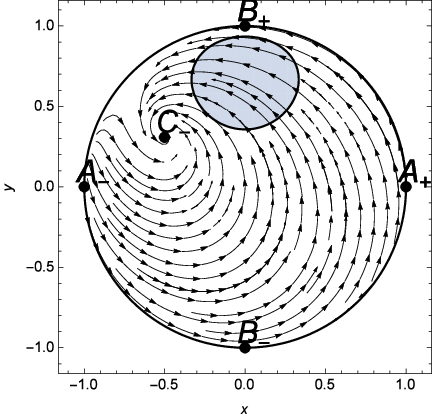
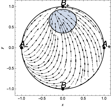
An important observation is that there is no critical point which represents a matter dominated epoch, corresponding to $\sigma=1$, located at the origin $(x,y)=(0,0)$ of the two dimensional system. However, all of the points $B_{\pm}$ and $C_{\pm}$ are scaling solutions and mimic the matter dominated EoS. We note that none of the critical points has an accelerating effective EoS, determined by the condition $w_{\rm eff}<-1/3$, and so a late time acceleration attractor solution is not possible. Thus the cosmology of this model can viably describe our universe if only very fine tuned initial conditions are imposed. In fact, there are regions in phase space in which acceleration can occur, but these periods of accelerations will be transitory. This means that setting the right initial conditions it might happen that a point in this accelerated region well describes the current observed state of the universe, thought, contrary to what predicted by $\Lambda$CDM, the expansion is doomed to decelerate again in the future. Although this might constitute a viable description of our universe, at least at the background level, it also introduces a fine tuning problem much worse that the one arising in $\Lambda$CDM.

For the remaining values of the parameters $\alpha$ and $\beta$, the system will be three dimensional and the variable $z$, defined in Eq. (36), will be required for the analysis. In this subsection we will analyse mathematically the dynamical system for various different combinations of choices for $\alpha$ and $\beta$ and look for physically interesting cosmology.

Many of the models studied so far in this section have either not possessed an accelerating critical point, or these critical points have not been generically stable. In order to look for more potentially viable cosmologies, in this subsection, we will consider the same extended chameleon models as above, but this time we will introduce a cosmological constant into the equations by taking the potential of the scalar field to be given by a simple positive constant, with $V(\phi)=\Lambda$. Note that a non-vanishing cosmological constant plus a quadratic effective potential of the kind (17), naturally arise from considering values near the minimum $\phi_{0}$ of some non linear effective potential, for example $V_{\rm eff}=\Lambda\cosh\left[m\left(\phi-\phi_{0}\right)/\sqrt{\Lambda}\right]$.

Adding $V(\phi)=\Lambda$ into the Friedmann equations modifies the dynamical system. We continue to work with the same variables $\sigma$, $x$ and $y$ as before, however this time it is more appropriate to introduce a redefined $z$, which we take to be

$\displaystyle z^{2}=\frac{\kappa^{2}\Lambda}{3H^{2}}.$

(44)

This modifies the Friedmann constraint as

$$1=\sigma^{2}+x^{2}+y^{2}+z^{2}\,.$$

(45)

From the definition of $z$ and the fact that we are working with a positive cosmological constant, we can restrict the analysis to consider only values $z\geq 0$. Again working with the variables $x$, $y$ and $z$, with $\sigma$ related to these variables algebraically via (45), means that the phase space for the dynamical system is simply the upper half unit sphere.

The dynamical system written in terms of these variables is

$$x^{\prime}=\frac{1}{2}\Bigg[-2x\gamma(w+1)yz^{1-\alpha-2\beta}\sigma^{\alpha+2\beta}\\ +3x\left(w\sigma^{2}+y^{2}(\alpha+\alpha w-1)-1\right)-3xz^{2}+3x^{3}-2\lambda y\sigma^{\alpha}z^{1-\alpha}\Bigg]$$

(46)

$$y^{\prime}=\frac{1}{2}\Bigg[-3y\left(\alpha-w\sigma^{2}-x^{2}+z^{2}+\alpha w-1\right)\\ +2z^{1-\alpha-2\beta}\sigma^{\alpha}\left(\gamma(w+1)\left(y^{2}+1\right)\sigma^{2\beta}+\lambda xz^{2\beta}\right)+3y^{3}(\alpha+\alpha w-1)\Bigg]$$

(47)

$$z^{\prime}=\frac{1}{2}\left[3z\left(w\sigma^{2}+y^{2}(\alpha+\alpha w-1)+x^{2}+1\right)-2\gamma(w+1)yz^{2-\alpha-2\beta}\sigma^{\alpha+2\beta}-3z^{3}\right],$$

(48)

where this time we have introduced the constants $\lambda$ and $\gamma$ as

$\displaystyle\lambda=\frac{\sqrt{3}\sqrt{A}\Lambda^{\frac{\alpha}{2}-\frac{1}{2}}}{\kappa},\quad\gamma=\frac{3\sqrt{A}\beta B\Lambda^{\frac{\alpha}{2}+\beta-\frac{1}{2}}}{\sqrt{2}}.$

(49)

In general the dynamical system will be singular on the $z=1$ plane if either of the conditions $\alpha>1$ or $\alpha+2\beta>1$ hold, in which case we will need to define a new time coordinate and multiply the right hand side of the dynamical system by an appropriate power of $z$ to describe the dynamics on this plane. The effective EoS (28) is given in terms of these variables as

$\displaystyle w_{\rm eff}=x^{2}+y^{2}(\alpha+\alpha w-1)-z^{2}+w\sigma^{2}-\frac{2}{3}\gamma(w+1)yz^{1-\alpha-2\beta}\sigma^{\alpha+2\beta}.$

(50)

Again, for general $\alpha$ and $\beta$, the system is practically impossible to analyse, however we can make a couple of comments. If $\alpha+2\beta>1$ then generically the effective EoS diverges on the $z=0$ plane. We can also observe that the matter dominated point $(0,0,0)$ is only a critical point of the dynamical system when the condition $\alpha+2\beta<1$ holds. In what follows we will restrict ourselves to particular physically interesting values of $\alpha$ and $\beta$ for a full analysis of the dynamical system.

We choose to work with a standard Newtonian gauge for which the line element can be written as

$\displaystyle ds^{2}=-(1+2\Phi)dt^{2}+\frac{(1-2\Psi)\,a(t)^{2}}{\left[1+\frac{1}{4}K\left(x^{2}+y^{2}+z^{2}\right)\right]^{2}}\left(dx^{2}+dy^{2}+dz^{2}\right)\,,$

(52)

where $x,y,z$ are Cartesian coordinates and $K=0,-1,1$ determines the spatial curvature of the universe. The scalar perturbations $\Phi$ and $\Psi$ are actually equal, due to the absence of anisotropies in the model under investigation. In fact the perturbed $ij$-components of the Einstein field equation yield

$\displaystyle\partial_{i}\partial_{j}\left[\left[1+\frac{1}{4}K\left(x^{2}+y^{2}+z^{2}\right)\right](\Psi-\Phi)\right]=0\,.$

(53)

which implies

$\displaystyle\Phi=\Psi\,.$

(54)

For this reason in the equations that follow we simply replace $\Phi$ in favour of $\Psi$ whenever it appears. Before displaying the equations we must first define the perturbed physical quantities: in particular the scalar field, the matter energy density, the matter pressure and the matter four-velocity are perturbed according to

$\displaystyle\phi+\delta\phi\,,\qquad\rho+\delta\rho\,,\qquad p+\delta p\,,\qquad u_{\mu}+\delta u_{\mu}\,,$

(55)

where the last term is defined in terms of the fluid’s perturbed scalar velocity $v$ by

$\displaystyle\delta u_{\mu}=\left(-\Psi,\partial_{i}v\right)\,.$

(56)

At this point we can present the perturbed equations.

References

- [1] Edmund J. Copeland, M. Sami, and Shinji Tsujikawa. Dynamics of dark energy. Int. J. Mod. Phys., D15:1753–1936, 2006. arXiv:hep-th/0603057.
- [2] M. Betoule et al. Improved cosmological constraints from a joint analysis of the SDSS-II and SNLS supernova samples. Astron. Astrophys., 568:A22, 2014. arXiv:1401.4064.
- [3] P. A. R. Ade et al. Planck 2015 results. XIII. Cosmological parameters. 2015. arXiv:1502.01589.
- [4] Steven Weinberg. The Cosmological Constant Problem. Rev. Mod. Phys., 61:1–23, 1989.
- [5] Jerome Martin. Everything You Always Wanted To Know About The Cosmological Constant Problem (But Were Afraid To Ask). Comptes Rendus Physique, 13:566–665, 2012. arXiv:1205.3365.
- [6] Ivaylo Zlatev, Li-Min Wang, and Paul J. Steinhardt. Quintessence, cosmic coincidence, and the cosmological constant. Phys. Rev. Lett., 82:896–899, 1999. arXiv:astro-ph/9807002.
- [7] Sean M. Carroll. Quintessence and the rest of the world. Phys. Rev. Lett., 81:3067–3070, 1998. arXiv:astro-ph/9806099.
- [8] Austin Joyce, Bhuvnesh Jain, Justin Khoury, and Mark Trodden. Beyond the Cosmological Standard Model. Phys. Rept., 568:1–98, 2015. arXiv:1407.0059.
- [9] Justin Khoury and Amanda Weltman. Chameleon fields: Awaiting surprises for tests of gravity in space. Phys. Rev. Lett., 93:171104, 2004. arXiv:astro-ph/0309300.
- [10] Justin Khoury and Amanda Weltman. Chameleon cosmology. Phys. Rev., D69:044026, 2004. arXiv:astro-ph/0309411.
- [11] A. I. Vainshtein. To the problem of nonvanishing gravitation mass. Phys. Lett., B39:393–394, 1972.
- [12] Kurt Hinterbichler and Justin Khoury. Symmetron Fields: Screening Long-Range Forces Through Local Symmetry Restoration. Phys. Rev. Lett., 104:231301, 2010. arXiv:1001.4525.
- [13] Kurt Hinterbichler, Justin Khoury, Aaron Levy, and Andrew Matas. Symmetron Cosmology. Phys. Rev., D84:103521, 2011. arXiv:1107.2112.
- [14] E. Babichev, C. Deffayet, and R. Ziour. k-Mouflage gravity. Int. J. Mod. Phys., D18:2147–2154, 2009. arXiv:0905.2943.
- [15] Philippe Brax and Patrick Valageas. K-mouflage Cosmology: the Background Evolution. Phys. Rev., D90(2):023507, 2014. arXiv:1403.5420.
- [16] Philippe Brax and Nicola Tamanini. Extended Chameleons. 2015. arXiv:1512.07399.
- [17] Christian G. Boehmer, Nicola Tamanini, and Matthew Wright. Interacting quintessence from a variational approach Part I: algebraic couplings. Phys. Rev., D91(12):123002, 2015. arXiv:1501.06540.
- [18] Christian G. Boehmer, Nicola Tamanini, and Matthew Wright. Interacting quintessence from a variational approach Part II: derivative couplings. Phys. Rev., D91(12):123003, 2015. arXiv:1502.04030.
- [19] Tomi S. Koivisto, Emmanuel N. Saridakis, and Nicola Tamanini. Scalar-Fluid theories: cosmological perturbations and large-scale structure. JCAP, 1509:047, 2015. arXiv:1505.07556.
- [20] Nicola Tamanini. Phenomenological models of dark energy interacting with dark matter. Phys. Rev., D92(4):043524, 2015. arXiv:1504.07397.
- [21] J. David Brown. Action functionals for relativistic perfect fluids. Class. Quant. Grav., 10:1579–1606, 1993. arXiv:gr-qc/9304026.
- [22] Christian G. Boehmer and Nyein Chan. Dynamical systems in cosmology. 2014. arXiv:1409.5585.
- [23] N. Tamanini. Dynamical systems in dark energy models. PhD thesis, University College London, 2014.
- [24] Christian G. Boehmer, Nyein Chan, and Ruth Lazkoz. Dynamics of dark energy models and centre manifolds. Phys. Lett., B714:11–17, 2012. arXiv:1111.6247.
- [25] Edmund J. Copeland, Andrew R Liddle, and David Wands. Exponential potentials and cosmological scaling solutions. Phys. Rev., D57:4686–4690, 1998. arXiv:gr-qc/9711068.
- [26] Artur Alho and Claes Uggla. Scalar field deformations of CDM cosmology. Phys. Rev., D92(10):103502, 2015. arXiv:1505.06903.
- [27] Christian G. Böhmer, Nicola Tamanini, and Matthew Wright. Einstein static universe in scalar-fluid theories. Phys. Rev., D92(12):124067, 2015. arXiv:1510.01477.
- [28] Philippe Brax and Patrick Valageas. K-mouflage Cosmology: Formation of Large-Scale Structures. Phys. Rev., D90(2):023508, 2014. arXiv:1403.5424.
- [29] Philippe Brax and Patrick Valageas. Small-scale Nonlinear Dynamics of K-mouflage Theories. Phys. Rev., D90(12):123521, 2014. arXiv:1408.0969.
- [30] Alexandre Barreira, Philippe Brax, Sebastien Clesse, Baojiu Li, and Patrick Valageas. Linear perturbations in K-mouflage cosmologies with massive neutrinos. Phys. Rev., D91:063528, 2015. arXiv:1411.5965.
- [31] Philippe Brax, Luca Alberto Rizzo, and Patrick Valageas. K-mouflage effects on clusters of galaxies. Phys. Rev., D92(4):043519, 2015. arXiv:1505.05671.
- [32] Anne-Christine Davis, Baojiu Li, David F. Mota, and Hans A. Winther. Structure Formation in the Symmetron Model. Astrophys. J., 748:61, 2012. arXiv:1108.3081.
- [33] Philippe Brax, Carsten van de Bruck, Anne-Christine Davis, Baojiu Li, Benoit Schmauch, and Douglas J. Shaw. Linear Growth of Structure in the Symmetron Model. Phys. Rev., D84:123524, 2011. arXiv:1108.3082.
- [34] Philippe Brax, Anne-Christine Davis, Baojiu Li, Hans A. Winther, and Gong-Bo Zhao. Systematic Simulations of Modified Gravity: Symmetron and Dilaton Models. JCAP, 1210:002, 2012. arXiv:1206.3568.