JOINT ML CALIBRATION AND DOA ESTIMATION WITH SEPARATED ARRAYS

Direction-of-arrival (DOA) estimation [1, 2] is an important topic with a large number of applications: radar, satellite, mobile communications, radio astronomy, geophysics and underwater acoustics [3, 4, 5]. In order to achieve high resolution, it is common to use arrays with large aperture and/or a large number of sensors, in a specific noise environment. Considering spatially and temporally uncorrelated zero-mean Gaussian processes is a typical noise assumption but it may be violated in numerous applications, as in the context of sonar, where correlated or colored noise is required [6, 7, 8, 9].

We consider here the case where the noise covariance matrix exhibits a particular (block-diagonal) structure [10] that differs from the classical assumption: spatially white uniform noise [11, 12] or non-uniform noise [13]. In our paper, we consider DOA estimation in large sensor arrays composed of multiple subarrays. Due to the large spacing between subarrays, we assume that the noise among sensors of different subarrays is statistically spatially independent. In a given subarray, however, the noise is spatially correlated between sensors. This entails a block-diagonal structure of the noise covariance matrix, linked to the sparsity of the array.

Apart from this noise assumption, we also consider that in realistic scenarios, due to miscalibration, the individual sensor outputs are generally subject to distortions by constant multiplicative complex factors (gains). These calibration errors are hardware related in our case, leading to different DOA independent sensor gains [14, 10]. To precisely estimate these errors, we take advantage of the presence of calibration sources [15, 16] to simultaneously calibrate and estimate DOAs. Our scenario is general and it can be adapted or extended to some practical applications as in the radio astronomy context [17] where the constant complex sensor gain assumption is common.

We use the conditional/deterministic model [18] for the signal sources. Nevertheless, following the same methodology, we can adapt the proposed algorithms to the case of unconditional/stochastic model [18, 19, 20, 21]. The two parametric algorithms we present are based on the maximum likelihood (ML) estimation method, due to its good statistical performances. The size of the unknown parameter vector being large, we perform iterative optimization to make the ML estimation problem computationally tractable. Furthermore, the estimation performances are improved with the introduction of calibration sources in our scenario. To assess the performances [22], the Cramér-Rao bound (CRB) is used.

The notation used through this paper is the following: scalars, vectors and matrices are represented by italic lower-case, boldface lower-case and boldface upper-case symbols, respectively. The symbols $\left(\cdot\right)^{T}$, $\left(\cdot\right)^{\ast}$, $\left(\cdot\right)^{H}$, $\left(\cdot\right)^{{\dagger}}$, $\mathrm{tr}\left\{\cdot\right\}$ and $\det\left\{\cdot\right\}$ denote, respectively, the transpose, the complex conjugate, the hermitian, the pseudo-inverse, the trace and determinant operator. The real and imaginary parts are referred to by $\Re\left\{\cdot\right\}$ and $\Im\left\{\cdot\right\}$. The operators $\mathrm{bdiag}\left\{\cdot\right\}$ and $\mathrm{diag}\left\{\cdot\right\}$ represent a block-diagonal and a diagonal matrix, respectively. A vector is by default a column vector and $\mathbf{I}$ is the identity matrix. The symbol $\odot$ denotes the Schur-Hadamard product, $\delta\left(.\right)$ is the Dirac’s delta function and $\mathbf{E}_{p}$ is a $p\times p$ matrix filled with ones.

We consider $D$ signal sources impinging on a linear (possibly not uniform) array of $M$ sensors. The array response vector for each source $l=1,\ldots,D$ is defined as [23]

in which $\theta_{l}$ is the DOA of the $l^{th}$ source, $f$ denotes the carrier frequency, $c$ the propagation speed and $d_{k}$ the inter-element spacing between the first and the $k^{th}$ sensor. We note as $\lambda$ the wavelength of the incident wave. The output observation of the full array is given at each snapshot by

where $N$ is the total number of snapshots, $\boldsymbol{\theta}=[\theta_{1},\ldots,\theta_{D}]^{T}$ is the DOAs vector, $\mathbf{s}(t)=[s_{1}(t),\ldots,s_{D}(t)]^{T}$ the signal source vector, $\mathbf{n}(t)=[n_{1}(t),\ldots,n_{M}(t)]^{T}$ the additive noise vector and $\mathbf{A}(\boldsymbol{\theta})=[\mathbf{a}(\theta_{1}),\ldots,\mathbf{a}(\theta_{D})]$ the array response matrix. In matrix notation, we have

with $\mathbf{Y}=[\mathbf{y}(1),\ldots,\mathbf{y}(N)]$, $\mathbf{S}=[\mathbf{s}(1),\ldots,\mathbf{s}(N)]$ and $\mathbf{N}=[\mathbf{n}(1),\ldots,\mathbf{n}(N)]$. In this work, the different assumptions that we consider are the following:

A1) Calibration sources: In a number of practical applications, the knowledge of one or multiple calibration sources is available [16, 24, 25, 26]. Without loss of generality, we consider the first $P$ sources as calibration sources with known DOAs. Thus, the steering matrix is partitioned as

in which $\boldsymbol{\theta}_{K}=[\mathbf{\theta}_{1},\ldots,\mathbf{\theta}_{P}]^{T}$ represents the known DOAs and $\boldsymbol{\theta}_{U}=[\mathbf{\theta}_{P+1},\ldots,\mathbf{\theta}_{D}]^{T}$ is the vector of the unknown DOAs. Likewise, the signal source matrix can be written as follows

in which $\mathbf{S}_{K}=[\mathbf{s}_{K}(1),\ldots,\mathbf{s}_{K}(N)]$, $\mathbf{S}_{U}=[\mathbf{s}_{U}(1),\ldots,\mathbf{s}_{U}(N)]$, $\mathbf{s}_{K}(t)=[s_{1}(t),\ldots,s_{P}(t)]^{T}$ and $\mathbf{s}_{U}(t)=[s_{P+1}(t),\ldots,s_{D}(t)]^{T}$.

A2) Complex unknown gains of each sensor: The instrumentation can introduce perturbations such as phase shifts, in particular due to the difference between sensor gains related to, e.g., receiver electronics. To correctly specify the model and avoid inaccurate estimations, calibration needs to be performed. This can be modeled using the following diagonal calibration matrix

where the vector $\mathbf{g}=[g_{1},\ldots,g_{M}]^{T}$ contains the different unknown complex gains [10, 5] which are modeled as DOA independent. Consequently, the observation matrix (3) can be rewritten as

A3) Geometry of sensor subarrays: In our scenario, the sensor array is constituted of a set of $L$ subarrays. Due to the large intersubarray distances with respect to the signal wavelength [27, 28], the noise is considered statistically independent between subarrays . Nevertheless, for a given subarray, sensors being closely spaced, the noise is assumed to be spatially correlated [10]. Thus, the noise covariance matrix denoted by $\boldsymbol{\Omega}$ has the following block-diagonal structure

in which $\boldsymbol{\Omega}_{i}$ is a $M_{i}\times M_{i}$ square matrix where $M_{i}$ is the number of sensors in the $i^{th}$ subarray, such that ${\sum}_{i=1}^{L}M_{i}=M$.

Vector of unknown parameters: Let us consider a deterministic/conditional model for the signal sources and zero-mean complex circular Gaussian noise so that

Consequently, the vector of unknown parameters is given by

in which for $i=1,\ldots,L$ and $h_{i},l_{i}=1,\ldots,M_{i}$, $\{[\boldsymbol{\Omega}_{i}]_{h_{i},l_{i}}\}_{l_{i}\geq h_{i}}$ represent all the non-zero elements in and above the diagonal of the noise covariance matrix.

In this section, we propose two schemes for joint array calibration and DOA estimation, based on an iterative ML algorithm [10, 13, 29]. The iterative procedure allows us to obtain a closed-form expression of the unknown complex gains, the unknown signal sources and the structured noise covariance matrix. Indeed, the log-likelihood function is optimized w.r.t. each unknown parameter, while fixing the others. The different closed-form expressions obtained are mutually dependent and require an iterative updating procedure with initialization. For the estimation of the unknown DOAs, an optimization procedure needs to be performed.

The presence of calibration sources and the iterative procedure allow us to reduce a $(D+2ND+{\sum}_{i=1}^{L}M_{i}^{2}+2M)$-dimensional optimization problem to a $(D-P)$-dimensional optimization problem. The main difference between the two proposed schemes lies in the estimation of the calibration matrix as it will be explained in the following.

In the following simulations, we consider two sources, a calibration source at $\theta_{1}=7^{\circ}$ and an unknown source at $\theta_{2}=15^{\circ}$, as well as 300 Monte-Carlo and $N=160$ snapshots. The full array is composed of 3 linear subarrays with 4, 3 and 2 sensors in each. The inter-element spacing is $\frac{\lambda}{2}$ in each subarray, 3$\lambda$ and $\frac{7\lambda}{2}$ between the three successive subarrays. We consider a noise covariance matrix $\boldsymbol{\Omega}$ with an identical noise power for each sensor of the same subarray. The amplitude gains and the phases are generated respectively uniformly on $\left[0,1\right]$ and $\left[0,2\pi\right]$.

The signal-to-noise ratio (SNR) is denoted by:

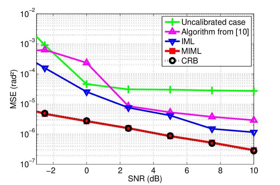
In Fig. 1, we plot the mean square error (MSE) vs. SNR, for both schemes, as well as for the uncalibrated case, meaning that the observations are given by (7) but estimation of matrix $\mathbf{G}$ is not performed in the estimation process, it is maintained equal to $\mathbf{I}$. In this case, we notice the degradation of performances, moreover the MSE is no longer decreasing from a certain value of the SNR. We also plot the MSE of the algorithm proposed in [10], for which the presence of calibration sources is not taken into account. As expected, the presence of a calibration source enables to achieve better performances, particularly with the MIML algorithm. The different computation times for the two exposed methods are 141.473 seconds for the IML algorithm (4 iterations) and 42.841 seconds for the MIML algorithm (2 iterations).

Finally, the Cramér-Rao bound (CRB) [10, 30, 31] was plotted. It is noticed that the best compromise between computation time and accuracy of estimation is achieved with the MIML algorithm. Indeed, we observe that numerically the MSE asymptotically reaches the CRB. Such performances are due to the estimation of the calibration matrix $\mathbf{G}$ which is performed separately from the estimation of $\boldsymbol{\theta}_{U}$ and mainly depends on the calibration sources ($\mathbf{A}(\boldsymbol{\theta}_{K})$ and $\mathbf{S}_{K}$), contrary to the first algorithm where it depends on the unknown sources as well ($\mathbf{A}(\boldsymbol{\theta})$ and $\mathbf{S}$). The IML algorithm requires more iterations to have better accuracy in the estimation.
Finally, Fig. 2 represents the MSE of the MIML algorithm for the two following cases: i) taking into account the true structure of the noise covariance matrix, and ii) assuming that the noise covariance matrix is diagonal. In the two cases, the observations are generated using the true noise covariance matrix which is structured as described by (8). As expected, such misspecification leads to a higher MSE (case ii) which shows the importance of taking into account the spatial correlation due to the array geometry.

In this paper, we proposed two iterative algorithms for joint calibration and DOA estimation. They are based on the ML estimation method and are applied in a particular context: some calibration sources are present, the sensors are characterized by unknown DOA independent complex gains and the noise covariance matrix has a block-diagonal structure. The MIML algorithm outperforms the IML algorithm and numerically attains the CRB for a low number of iterations. The proposed algorithm is general and can be adapted, for example, in the context of radio astronomy.

References

- [1] M. Haardt, M. Pesavento, F. Roemer, and M. N. El Korso, “Subspace methods and exploitation of special array structures,” in Electronic Reference in Signal Processing: Array and Statistical Signal Processing (M. Virberg, ed.). Academic Press Library in Signal Processing, Elsevier Ltd., 2014, vol. 3.
- [2] P. Stoica and K. C. Sharman, “Maximum likelihood methods for direction-of-arrival estimation,” IEEE Trans. Acoust., Speech, Signal Processing, vol. 38, no. 7, pp. 1132–1143, 1990.
- [3] L. C. Godara, “Application of antenna arrays to mobile communications, part II: Beam-forming and direction-of-arrival considerations,” Proceedings of the IEEE, vol. 85, no. 8, pp. 1195–1245, 1997.
- [4] K. T. Wong and M. D. Zoltowski, “Root-MUSIC-based azimuth-elevation angle-of-arrival estimation with uniformly spaced but arbitrarily oriented velocity hydrophones,” IEEE Trans. Signal Processing, vol. 47, no. 12, pp. 3250–3260, 1999.
- [5] A.-J. van der Veen and S. J. Wijnholds, “Signal processing tools for radio astronomy,” in Handbook of Signal Processing Systems. Springer, 2013, pp. 421–463.
- [6] H. Ye and R. D. DeGroat, “Maximum likelihood DOA estimation and asymptotic Cramér-Rao bounds for additive unknown colored noise,” IEEE Trans. Signal Processing, vol. 43, no. 4, pp. 938–949, 1995.
- [7] B. Friedlander and A. J. Weiss, “Direction finding using noise covariance modeling,” IEEE Trans. Signal Processing, vol. 43, no. 7, pp. 1557–1567, 1995.
- [8] P. Stoica, M. Viberg, K. M. Wong, and Q. Wu, “Maximum-likelihood bearing estimation with partly calibrated arrays in spatially correlated noise fields,” IEEE Trans. Signal Processing, vol. 44, no. 4, pp. 888–899, 1996.
- [9] M. Li and Y. Lu, “Maximum likelihood DOA estimation in unknown colored noise fields,” IEEE Trans. Aerosp. Electron. Syst., vol. 44, no. 3, pp. 1079–1090, 2008.
- [10] S. Vorobyov, A. B. Gershman, and K. M. Wong, “Maximum likelihood direction-of-arrival estimation in unknown noise fields using sparse sensor arrays,” IEEE Trans. Signal Processing, vol. 53, no. 1, pp. 34–43, 2005.
- [11] P. Stoica and A. Nehorai, “Performance study of conditional and unconditional direction-of-arrival estimation,” IEEE Trans. Acoust., Speech, Signal Processing, vol. 38, no. 10, pp. 1783–1795, 1990.
- [12] M. N. El Korso, G. Bouleux, R. Boyer, and S. Marcos, “Sequential estimation of the range and the bearing using the zero-forcing MUSIC approach,” in 17th European Signal Processing Conf., Glasgow, Scotland, 2009.
- [13] M. Pesavento and A. B. Gershman, “Maximum-likelihood direction-of-arrival estimation in the presence of unknown nonuniform noise,” IEEE Trans. Signal Processing, vol. 49, no. 7, pp. 1310–1324, 2001.
- [14] A. J. Weiss and B. Friedlander, “Eigenstructure methods for direction finding with sensor gain and phase uncertainties,” Circuits, Syst., Signal Process., vol. 9, no. 3, pp. 271–300, 1990.
- [15] J. Pierre and M. Kaveh, “Experimental performance of calibration and direction-finding algorithms,” in Proc. of IEEE Int. Conf. Acoust., Speech, Signal Processing, Toronto, Ontario, Canada, 1991, pp. 1365–1368.
- [16] B. C. Ng and C. M. S. See, “Sensor-array calibration using a maximum-likelihood approach,” IEEE Trans. Antennas Propag., vol. 44, no. 6, pp. 827–835, 1996.
- [17] S. J. Wijnholds, “Fish-eye observing with phased array radio telescopes,” Ph.D. dissertation, Technische Universiteit Delft, Delft, The Netherlands, 2010.
- [18] B. Ottersten, M. Viberg, P. Stoica, and A. Nehorai, “Exact and large sample maximum likelihood techniques for parameter estimation and detection in array processing,” in Radar Array Processing, S. Haykin, J. Litva, and T. J. Shepherd, Eds. Berlin: Springer-Verlag, 1993, ch. 4, pp. 99–151.
- [19] P. Stoica and A. Nehorai, “On the concentrated stochastic likelihood function in array signal processing,” Circuits, Syst., Signal Process., vol. 14, no. 5, pp. 669–674, 1995.
- [20] A. Gershman, P. Stoica, M. Pesavento, and E. G. Larsson, “Stochastic Cramér-Rao bound for direction estimation in unknown noise fields,” IEE Proceedings-Radar, Sonar and Navigation, vol. 149, no. 1, pp. 2–8, 2002.
- [21] C. E. Chen, F. Lorenzelli, R. E. Hudson, and K. Yao, “Stochastic maximum-likelihood DOA estimation in the presence of unknown nonuniform noise,” IEEE Trans. Signal Processing, vol. 56, no. 7, pp. 3038–3044, 2008.
- [22] M. N. El Korso, R. Boyer, A. Renaux, and S. Marcos, “Conditional and unconditional Cramér-Rao bounds for near-field source localization,” IEEE Trans. Signal Processing, vol. 58, no. 5, pp. 2901–2907, 2010.
- [23] H. Krim and M. Viberg, “Two decades of array signal processing research: The parametric approach,” IEEE Signal Processing Mag., vol. 13, no. 4, pp. 67–94, 1996.
- [24] R. Boyer and G. Bouleux, “Oblique projections for direction-of-arrival estimation with prior knowledge,” IEEE Trans. Signal Processing, vol. 56, no. 4, pp. 1374–1387, 2008.
- [25] G. Bouleux, P. Stoica, and R. Boyer, “An optimal prior-knowledge-based DOA estimation method,” in 17th European Signal Processing Conf., Glasgow, United Kingdom, 2009, pp. 869–873.
- [26] M. N. El Korso, R. Boyer, and S. Marcos, “Fast sequential source localization using the projected companion matrix approach,” in Proceedings of the 3rd IEEE International Workshop on Computational Advances in Multi-Sensor Adaptive Processing, Aruba, Dutch Antilles, The Netherlands, 2009, pp. 245–248.
- [27] M. D. Zoltowski and K. T. Wong, “Closed-form eigenstructure-based direction finding using arbitrary but identical subarrays on a sparse uniform Cartesian array grid,” IEEE Trans. Signal Processing, vol. 48, no. 8, pp. 2205–2210, 2000.
- [28] M. Pesavento, A. B. Gershman, and K. M. Wong, “Direction of arrival estimation in partly calibrated time-varying sensor arrays,” in Proc. of IEEE Int. Conf. Acoust., Speech, Signal Processing, Salt Lake City, UT, 2001, pp. 3005–3008.
- [29] X. Zhang, M. N. El Korso, and M. Pesavento, “Maximum likelihood and maximum a posteriori direction-of-arrival estimation in the presence of SIRP noise,” in Proc. of IEEE Int. Conf. Acoust., Speech, Signal Processing, Shanghai, China, 2016.
- [30] P. Stoica and R. L. Moses, Spectral analysis of signals. Pearson/Prentice Hall Upper Saddle River, NJ, 2005.
- [31] A. L. Matveyev, A. B. Gershman, and J. F. Böhme, “On the direction estimation Cramér-Rao bounds in the presence of uncorrelated unknown noise,” Circuits, Syst., Signal Process., vol. 18, no. 5, pp. 479–487, 1999.