Principal Component Projection
Without Principal Component Analysis
Roy Frostig
Affiliation: Stanford University
Email: rf@cs.stanford.eduCameron Musco
Affiliation: MIT
Email: cnmusco@mit.eduChristopher Musco
Affiliation: MIT
Email: cpmusco@mit.eduAaron Sidford
Affiliation: Microsoft Research, New England
Email: asid@microsoft.com
February 23, 2016
Abstract
We show how to efficiently project a vector onto the top principal
components of a matrix, without explicitly computing these
components. Specifically, we introduce an iterative algorithm that
provably computes the projection using few calls to any black-box
routine for ridge regression.
By avoiding explicit
principal component analysis (PCA), our algorithm is the first with no runtime dependence on the number of
top principal components.
We show that it can be used to give a fast iterative method for the popular
principal component regression problem, giving the first major
runtime improvement over the naive method of combining
PCA with regression.
To achieve our results, we first observe that ridge regression can be used to obtain a “smooth projection” onto the top principal components. We then sharpen this approximation to true projection using a low-degree polynomial approximation to the matrix step function.
Step function approximation is a topic of long-term interest in
scientific computing. We extend prior theory by constructing
polynomials with simple iterative structure and rigorously analyzing their behavior under limited precision.
1 Introduction
In machine learning and statistics, it is common – and often
essential – to represent data in a concise form that decreases noise and increases
efficiency in downstream tasks. Perhaps the most
widespread method for doing so is to project data onto the linear subspace spanned by
its directions of highest variance – that is, onto the span of the top
components given by principal component analysis (PCA).
Computing principal components can be an expensive task, a challenge that prompts
a basic algorithmic question:
Can we project a vector onto the span of a matrix’s top principal components without performing principal component analysis?
This paper answers that question in the affirmative, demonstrating that projection
is much easier than PCA itself. We show that it can be solved using a simple iterative algorithm
based on black-box calls to a ridge regression routine.
The algorithm’s runtime does not depend on the number of top principal components chosen for projection, a cost inherent to any algorithm for PCA, or even algorithms that just compute an orthogonal span for the top components.
1.1 Motivation: principal component regression
To motivate our projection problem, consider one of the most basic downstream
applications for PCA: linear regression. Combined, PCA and regression
comprise the principal component regression (PCR) problem:
Let be a design matrix whose rows are data points and let be a vector of data labels.
Let denote the result of projecting each row of onto the span of the top principal components of – in particular the eigenvectors
of the covariance matrix whose corresponding variance (eigenvalue) exceeds a threshold . The
task of PCR is to find a minimizer of the squared loss
. In other words, the goal is to
compute , where
is the Moore-Penrose pseudoinverse of .
PCR is a key regularization method in statistics,
numerical linear algebra, and scientific disciplines including chemometrics
[Hot57, Han87, FF93].
It
models the assumption that small principal components represent noise
rather than data signal.
PCR is typically solved by first using PCA to compute and then applying
linear regression. The PCA step dominates the algorithm’s cost, especially if many principal components have
variance above the threshold .
We remedy this issue by showing that our principal component projection algorithm yields a fast algorithm for regression. Specifically,
full access to is unnecessary for PCR: can be computed efficiently given only an approximate projection of the vector onto ’s top principal components. By solving projection without PCA we obtain the first PCA-free algorithm for PCR.
1.2 A first approximation: ridge regression
Interestingly, our main approach to efficient principal component projection
is based on a common alternative to PCR: ridge regression.
This ubiquitous regularization method computes a
minimizer of for some regularization parameter [Tik63].
The advantage of ridge regression is its formulation as a simple
convex optimization problem that can be solved efficiently using many techniques (see Lemma 2.1).
Solving ridge regression is equivalent to applying the matrix , an
operation that can be viewed as a smooth relaxation of PCR.
Adding the norm penalty (i.e. ) effectively “washes out” ’s small principal components in
comparison to its large ones and achieves an
effect similar to PCR at the extreme ends of ’s spectrum.
Accordingly, ridge regression gives access to a “smooth projection”
operator, . This
matrix approximates , the projection matrix
onto ’s top principal components. Both have the same singular
vectors, but has a singular value of for
each squared singular value in and
a singular value of for each , whereas
has singular
values equal to . This
function approaches when is much greater than
and when it is smaller. Figure 1
illustrates the comparison.
Figure 1: Singular values of the projection matrix vs. those of the smooth projection operator obtained from ridge regression.
Unfortunately, ridge regression is a very crude approximation to
PCR and projection in many settings and may perform significantly
worse in certain data analysis applications [DFKU13]. In
short, while ridge regression algorithms are valuable tools, it has
been unclear how to wield them for tasks like projection or PCR.
1.3 Main result: from ridge regression to projection
We show that it is possible to sharpen the weak approximation given by ridge regression.
Specifically, there exists a low degree
polynomial such that provides a very accurate approximation to for any vector .
Moreover, the polynomial can be evaluated as a recurrence,
which translates into a simple iterative algorithm: we can apply the sharpened
approximation to a vector by repeatedly applying
any ridge regression routine a small number of times.
Theorem 1.2(Principal component projection without PCA).
Given and , Algorithm 1 uses approximate applications of and returns with .
Like most iterative PCA algorithms, our running time scales
inversely with , the spectral gap around .
Notably, it does not depend
on the number of principal components in ,
a cost incurred by any method that applies the projection directly, either by explicitly computing the top principal components of , or even by just computing an orthogonal span for these components.
As mentioned, the above theorem also yields an algorithm for principal component regression that computes without finding . We achieve this result by introducing a robust reduction from projection to PCR, that again relies on ridge regression as a computational primitive.
Corollary 1.3(Principal component regression without PCA).
Given and , Algorithm 2 uses approximate applications of and returns with .
Corollary 1.3 gives the first known algorithm
for PCR that avoids the cost of principal component analysis.
1.4 Related work
A number of papers attempt to alleviate the high cost of principal component analysis when
solving PCR. It has been shown that an approximation to
suffices for solving the regression problem [CH90, BMI14].
Unfortunately, even the fastest approximations are much slower than routines for ridge regression and
inherently incur a linear dependence on the number of principal components above .
More closely related to our approach is work on the matrix sign function, an important operation in control theory, quantum chromodynamics, and scientific computing in general.
Approximating the sign function often involves matrix polynomials
similar to our “sharpening polynomial” that converts ridge regression to principal component projection. Significant effort addresses Krylov methods for applying
such operators without computing them explicitly [vdEFL+02, FS08].
Our work differs from these methods in an important way: since we only assume access to an approximate ridge regression algorithm, it is essential that our sharpening step is robust to noise. Our iterative polynomial construction allows for a complete and rigorous noise analysis that is not available for Krylov methods, while at the same time eliminating space and post-processing costs.
Iterative approximations to the matrix sign function have been proposed, but lack rigorous noise analysis [Hig08].
1.5 Paper layout
Section 2: Mathematical and algorithmic preliminaries.
Section 3: Develop a PCA-free algorithm for principal component projection based on a ridge regression subroutine.
Section 4: Show how our approximate projection algorithm can be used to solve PCR, again without PCA.
Section 5: Detail our iterative approach to sharpening the smooth ridge regression projection towards true projection via a low degree sharpening polynomial.
Section 6: Empirical evaluation of our principal component projection and regression algorithms.
2 Preliminaries
Singular value decomposition.
Any matrix of rank has a
singular value decomposition (SVD) , where
and both have orthonormal columns
and is a diagonal matrix. The columns of
and are the left and right singular vectors of
. Moreover, , where are the
singular values of in decreasing order.
The columns of are the eigenvectors of the covariance matrix
, i.e. the principal components of the data,
and the eigenvalues of the covariance matrix are the squares of the
singular values .
Functions of matrices.
If is a scalar function and is a diagonal matrix, we define by the entrywise application of to the diagonal. For a non-diagonal matrix with SVD we define .
Matrix pseudoinverse.
We define the pseudoinverse of as
where . The
pseudoinverse is essential in the context of regression, as the vector
minimizes the squared error .
Principal component projection.
Given a threshold let be the largest index
with and define:
The matrix contains ’s rows projected to the
span of all principal components having squared singular value at
least . We sometimes write where is the projection onto these top components. Here
where is a step
function: if and if .
Miscellaneous notation.
For any positive semidefinite we use to denote that is positive semidefinite. For any , .
Ridge regression.
Ridge regression is the problem of computing, given a regularization
parameter :
(1)
The solution to (1) is given by . Applying the matrix to is equivalent to solving the convex minimization problem:
for .
A vast literature studies solving problems of this form via (accelerated) gradient descent, stochastic variants, and random sketching [Nes83, NN13, SSZ14, LLX14, FGKS15, CLM+15].
We summarize a few, now standard, runtimes achievable by these iterative methods:
Lemma 2.1(Ridge regression runtimes).
Given let
There is an algorithm,
that, for any , returns
such that
It
runs in time where is the condition
number of the regularized system and is the number of
nonzero entries in . There is a also stochastic algorithm that, for
any , gives the same guarantee with probability
in time
where
is ’s stable rank.
When the runtime can be improved to
where the hides a factor of .
Typically, the regularized condition number will be significantly smaller than the full condition number of .
3 From ridge regression to principal component projection
We now describe how to approximately apply
using any black-box ridge regression routine. The key idea is to first
compute a soft step function of via ridge
regression, and then to sharpen this step to approximate
.
Let be the result of applying ridge regression to
. In the language of functions of matrices,
we have , where
The function is a smooth step about (see Figure
1). It primarily serves to map the eigenvalues of
to the range , mapping those exceeding the
threshold to a value above and the rest to a value
below .
To approximate the projection , it would
now suffice to apply a simple symmetric step function:
It is easy to see that . For , and so
. Similarly for , and hence
. That is, the symmetric step function exactly converts
our smooth ridge regression step to the true projection operator.
3.1 Polynomial approximation to the step function
While computing directly is expensive, requiring the SVD of , we show how to approximate this function with a low-degree polynomial. We also show how to apply this polynomial efficiently and stably using a simple iterative algorithm. Our main result, proven in Section 5, is:
Lemma 3.1(Step function algorithm).
Let be symmetric with every eigenvalue satisfying and . Let denote a procedure that on produces with . Given set
, , and for set
and . If all arithmetic operations are performed with bits of precision then
for .
Note that the output is an approximation to a degree polynomial of applied to .
In Algorithm 1, we give pseudocode for combining the procedure with ridge regression to solve principal component projection.
Set and let be an algorithm that approximately applies to any by applying approximate ridge regression to . As long as has no eigenvalues falling within of , the lemma ensures . This requires on order of the spectral gap: , where is the largest index with .
Algorithm 1 (pc-proj) Principal component projection
input: , , error , failure rate , threshold , gap
,
fordo
endfor
return
Theorem 3.2.
If and are sufficiently large constants, pc-proj (Algorithm 1) returns such that with probability ,
The algorithm requires ridge regression calls, each costing . Lemma 2.1 yields total cost (with no failure probability)
or, via stochastic methods,
with acceleration possible when .
Proof.
We instantiate Lemma 3.1. Let . As discussed, and hence all its eigenvalues fall in . Specifically, . Now, and similarly , so all eigenvalues of are at least far from .
By Lemma 2.1, for any , with probability :
Since the minimum eigenvalue of is :
Applying the union bound over all calls of ridge, this bound holds for all calls with probability
So, overall, by Lemma 3.1, with probability at least , . As discussed, . Adjusting constants on (via and ) completes the proof.
∎
Note that the runtime of Theorem 3.2 includes a dependence on . In performing principal component projection, pc-proc applies an asymmetric step function to . The optimal polynomial for approximating this step also has a dependence [EY11], showing that our reduction from projection to ridge regression is optimal in this regard.
3.2 Choosing and
Theorem 3.2 requires If is chosen approximately equidistant from the two eigenvalues, we need .
In practice, however, it is unnecessary to explicitly specify or to choose so precisely. With our projection will be approximately correct on all singular values outside the range . If there are any “intermediate” singular values in this range, as shown in Section 5, the approximate step function applied by Lemma 3.1 will map these values to via a monotonically increasing soft step. That is, Algorithm 1 gives a slightly softened projection – removing any principal directions with value , keeping any with value and partially projecting away any in between.
4 From principal component projection to principal component regression
A major motivation for an efficient, PCA-free method for projecting a vector onto the span of top principal components is principal component regression (PCR). Recall that PCR solves the following problem:
In exact arithmetic, is equal to .
This identity suggests a method for computing the solution to ridge regression without finding explicitly: first apply a principal component projection algorithm to and then solve a linear system to apply .
Unfortunately, this approach is disastrously unstable, not only when is applied approximately, but in any finite precision environment. Accordingly, we present a modified method for obtaining PCA-free regression from projection.
4.1 Stable inversion via ridge regression
Let and suppose we
have some (e.g. obtained from
Algorithm 1). The issue with the first approach mentioned
is that since could have a very large maximum
eigenvalue, we cannot guarantee . On the other hand, applying the
ridge regression operator to
is much more stable since it has a maximum eigenvalue
of , so
will approximate well.
In short, it is more stable to apply , where , but the goal in PCR is to apply
where .
So, in order to go from one function to the other, we use a correction
function . By simple calculation,
Additionally, we can stably approximate with an iteratively
computed low degree polynomial! Specifically, we use a truncation of
the series An exact
approximation to would exactly apply ,
which as discussed, is unstable due to very large eigenvalues
(corresponding to small eigenvalues of ). Our
approximation to is accurate on the large eigenvalues of
but inaccurate on the small
eigenvalues. This turns out to be the key to the stability of our
algorithm. By not “fully inverting” these eigenvalues, our
polynomial approximation avoids the instability of applying the true
inverse . We provide a complete error analysis in
Appendix B, the upshot of which is the following:
Lemma 4.1(PCR approximation algorithm).
Let be a procedure that, given , produces with . Let be a procedure that, given produces with . Given set and . For set:
If all arithmetic operations are performed with bits of precision then
for .
We instantiate the iterative procedure above in Algorithm 2. denotes a call to Algorithm 1.
If and are sufficiently large constants, ridge-pcr (Algorithm 2) returns such that with probability ,
The algorithm makes one call to pc-proj and calls to ridge regression, each of which costs , so
Lemma 2.1 and Theorem 3.2 imply a total runtime of
where hides , or, with stochastic methods,
Proof.
We apply Lemma 4.1; is given by . Since , Lemma 2.1 states that with probability ,
Now, is given by . With probability , if then by Theorem 3.2,
Applying the union bound over calls to and a single call to , these bounds hold on every call with probability . Adjusting constants on (via and ) proves the theorem.
∎
5 Approximating the matrix step function
We now return to proving our underlying result on iterative polynomial approximation of the matrix step function:
Let be symmetric with every eigenvalue satisfying and . Let denote a procedure that on produces with . Given set
, , and for set
and . If all arithmetic operations are performed with bits of precision and if then
.
The derivation and proof of Lemma 3.1 is split into 3 parts. In Section 5.1 we derive a simple low degree polynomial approximation to the sign function:
In Section 5.2 we show how this polynomial can be computed with a stable iterative procedure. In Section 5.3 we use these pieces and the fact that the step function is simply a shifted and scaled sign function to prove Lemma 3.1.
Along the way we give complementary views of
Lemma 3.1 and show that there exist more
efficient polynomial approximations.
5.1 Polynomial approximation to the sign function
We show that for sufficiently large , the following polynomial is
uniformly close to on :
The polynomial can be derived in several ways. One follows
from observing that is odd and thereby is even. So, a good polynomial approximation for should
be odd and, when divided by , should be even (i.e. a function of
). Specifically, given a polynomial approximation to
on the range we can approximate using
. Choosing to be the -th order Taylor approximation
to at yields . With this insight we
show that converges to .
Lemma 5.1.
for all .
Proof.
Let . By induction on it is straightforward to show that the -th derivative of at is
Since we see that the degree Taylor approximation to at is therefore
Note that for , the remainder has absolute value at most . Therefore
the remainder converges to as and the
Taylor approximation converges, i.e. for . Since we have for with . Since
, the result follows.
∎
Alternatively, to derive we can consider , which is relatively large near and small on the rest of . Integrating this function from to and normalizing yields a good step function. In Appendix A we prove that:
Lemma 5.2.
For all
Next, we bound the rate of convergence of to :
Lemma 5.3.
For if then and
(2)
If then and
Proof.
The claim is trivial when . Since is odd it suffices
to consider . For such , it is direct that , and follows from the observation that
increases monotonically with and by Lemma 5.1. All
that remains to show is the left-side inequality of
(2). Using
Lemma 5.1 again,
Now since for all and , we have
Combining with and again
that proves the left hand side of
(2).
∎
The lemma directly implies that is a high quality approximation to for bounded away from .
Corollary 5.4.
If , with and , then .
We conclude by noting that this proof in fact implies the existence of
a lower-degree polynomial approximation to . Since the sum of coefficients in our expansion is small, we can replace each with Chebyshev polynomials of lower degree. In
Appendix A, we prove:
Lemma 5.5.
There exists an degree polynomial such that for all with .
Lemma 5.5 achieves, up an additive
, the optimal trade off between degree and
approximation of [EY07]. We have preliminary progress toward making this near-optimal polynomial algorithmic, a topic we leave to explore in future work.
5.2 Stable iterative algorithm for the sign function
We now provide an iterative algorithm for computing that works when applied with limited precision. Our formula is obtained by considering each term of . Let
Clearly and therefore we can compute the iteratively. Since we can compute iteratively as well. We show this procedure works when applied to matrices, even if all operations are performed with limited precision:
Lemma 5.6.
Let be symmetric with . Let be a procedure that given produces with
Given suppose that we have and such that and . For all set
Then if arithmetic operations are carried out with bits of precision we have for
Proof.
Let , , and . Since and we see that even if and are truncated to the given bit precision we still have and .
Now suppose that for some . Since for and we know that and by reverse triangle inequality . Using our assumption on and applying triangle inequality yields
In the last line we used since . Again, by this fact we know that and therefore again by reverse triangle inequality . Using to compute with bounded arithmetic precision will then introduce an additional additive error of . Putting all this together we have that grows by at most an additive every time increases and by the same argument so does . Including our initial error of on and , we conclude that and are both bounded by .
∎
5.3 Approximating the step function
We finally apply the results of Section 5.1 and Section 5.2 to approximate the step function and prove Lemma 3.1. We simply apply the fact that and perform further error analysis. We first use Lemma 5.6 to show how to compute .
Lemma 5.7.
Let be symmetric with . Let be a procedure that on produces with . Given arbitrary set , , and for all set
and . If arithmetic operations are performed with bits of precision and then
.
Proof.
Since we see that is the same as in Lemma 5.6 with and , and . Since multiplying by everywhere does not increase error and since we can invoke Lemma 5.6 to yield the result provided we can show
.
Computing and subtracting from introduces at most additive error Consequently by the error guarantee of , as desired.
∎
Using Lemma 5.7 and Corollary 5.4 we finally have:
By assumption, and .
Invoking Lemma 5.7 with error , letting we have
(3)
Now, since and every eigenvalue of is in , by assumption on we can invoke Corollary 5.4 yielding
The result follows from combining with (3) via triangle inequality.
∎
6 Empirical evaluation
We conclude with an empirical evaluation of pc-proc and
ridge-pcr (Algorithms 1 and 2).
Since PCR has already been justified as a statistical technique, we
focus on showing that, with few iterations, the algorithm recovers
an accurate approximation to and
.
We begin with synthetic data, which lets us control the spectral gap that dominates our iteration bounds (see Theorem 3.2).
Data is generated randomly by drawing top singular values uniformly from the range and tail singular values from . is set to and is formed via the SVD where and are random orthonormal matrices and contains our random singular values. To model a typical PCR application, is generated by adding noise to the response of a random “true” that correlates with ’s top principal components.
(a)Regression
(b)Projection
Figure 2: Relative error (shown on log scale) for ridge-pcr and pc-proj for synthetically generated data.
As apparent in Figure 2(a), our algorithm performs very well for regression, even for small . Error is measured via the natural -norm and we plot
.
Figure 2(b) shows similar convergence for projection, although we do notice a stronger effect of a small gap in this case.
Projection error is given with respect to the more natural 2-norm.
Both plots confirm the linear convergence predicted by our analysis (Theorems 3.2 and 4.2).
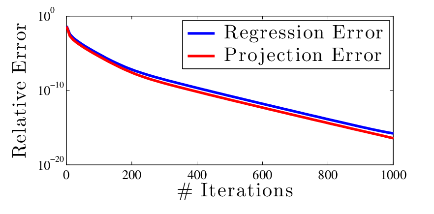
To illustrate stability, we include an extended plot for the data which shows arbitrarily high accuracy as iterations increase (Figure 3).
Figure 3: Extended log error plot on synthetic data with gap .
Finally, we consider a large regression problem constructed from MNIST classification data [LCB15], with the goal of distinguishing handwritten digits {1,2,4,5,7} from the rest.
Input is normalized and 1000 random Fourier features are generated according to a unit RBF kernel [RR07]. Our final data set is both of larger scale and condition number than the original.
Figure 4: Relative error (on log scale) for ridge-pcr and pc-proj for an MNIST-based regression problem.
The MNIST principal component regression was run with . Although the gap is very small around this
cutoff point (just ), we see fast convergence for
PCR. Convergence for projection is slowed more notably by the small
gap, but it is still possible to obtain relative error with
only 20 iterations (i.e. invocations of ridge regression).
References
[BMI14]
Christos Boutsidis and Malik Magdon-Ismail.
Faster SVD-truncated regularized least-squares.
In Proceedings of the 2014 IEEE International Symposium on Information Theory (ISIT), pages 1321–1325, 2014.
[CH90]
Tony F. Chan and Per Christian Hansen.
Computing truncated singular value decomposition least squares
solutions by rank revealing qr-factorizations.
SIAM Journal on Scientific and Statistical Computing,
11(3):519–530, 1990.
[CLM+15]
Michael B. Cohen, Yin Tat Lee, Cameron Musco, Christopher Musco, Richard Peng,
and Aaron Sidford.
Uniform sampling for matrix approximation.
In Proceedings of the 6th Conference on Innovations in Theoretical Computer Science (ITCS), pages 181–190, 2015.
[DFKU13]
Paramveer S. Dhillon, Dean P. Foster, Sham M. Kakade, and Lyle H. Ungar.
A risk comparison of ordinary least squares vs ridge regression.
The Journal of Machine Learning Research, 14(1):1505–1511,
2013.
[EY07]
Alexandre Eremenko and Peter Yuditskii.
Uniform approximation of by polynomials and entire
functions.
Journal d’Analyse Mathématique, 101(1):313–324, 2007.
[EY11]
Alexandre Eremenko and Peter Yuditskii.
Polynomials of the best uniform approximation to on two
intervals.
Journal d’Analyse Mathématique, 114(1):285–315, 2011.
[FF93]
Ildiko E. Frank and Jerome H. Friedman.
A statistical view of some chemometrics regression tools.
Technometrics, 35(2):109–135, 1993.
[FGKS15]
Roy Frostig, Rong Ge, Sham M. Kakade, and Aaron Sidford.
Un-regularizing: approximate proximal point and faster stochastic
algorithms for empirical risk minimization.
In Proceedings of the 32nd International Conference on Machine Learning (ICML), 2015.
[FS08]
Andreas Frommer and Valeria Simoncini.
Model Order Reduction: Theory, Research Aspects and
Applications, chapter Matrix Functions, pages 275–303.
Springer Berlin Heidelberg, Berlin, Heidelberg, 2008.
[Han87]
Per Christian Hansen.
The truncated SVD as a method for regularization.
BIT Numerical Mathematics, 27(4):534–553, 1987.
[Hig08]
Nicholas J. Higham.
Functions of Matrices: Theory and Computation.
Society for Industrial and Applied Mathematics, 2008.
[Hot57]
Harold Hotelling.
The relations of the newer multivariate statistical methods to factor
analysis.
British Journal of Statistical Psychology, 10(2):69–79, 1957.
[LCB15]
Yann LeCun, Corinna Cortes, and Christopher J.C. Burges.
MNIST handwritten digit database.
2015.
[LLX14]
Qihang Lin, Zhaosong Lu, and Lin Xiao.
An accelerated proximal coordinate gradient method.
In Advances in Neural Information Processing Systems 27 (NIPS), pages 3059–3067, 2014.
[Nes83]
Yurii Nesterov.
A method for unconstrained convex minimization problem with the rate
of convergence .
In Soviet Mathematics Doklady, volume 27, pages 372–376, 1983.
[NN13]
Jelani Nelson and Huy L. Nguyên.
OSNAP: Faster numerical linear algebra algorithms via sparser
subspace embeddings.
In Proceedings of the 54th Annual IEEE Symposium on Foundations of Computer Science (FOCS), pages 117–126, 2013.
[RR07]
Ali Rahimi and Benjamin Recht.
Random features for large-scale kernel machines.
In Advances in Neural Information Processing Systems 20 (NIPS), pages 1177–1184. 2007.
[SSZ14]
Shai Shalev-Shwartz and Tong Zhang.
Accelerated proximal stochastic dual coordinate ascent for
regularized loss minimization.
Mathematical Programming, pages 1–41, 2014.
[SV14]
Sushant Sachdeva and Nisheeth K. Vishnoi.
Faster algorithms via approximation theory.
Foundations and Trends in Theoretical Computer Science,
9(2):125–210, 2014.
[Tik63]
Andrey Tikhonov.
Solution of incorrectly formulated problems and the regularization
method.
In Soviet Mathematics Doklady, volume 4, pages 1035–1038,
1963.
[vdEFL+02]
Jasper van den Eshof, Andreas Frommer, Thomas Lippert, Klaus Schilling, and
Henk A. van der Vorst.
Numerical methods for the QCD overlap operator I: Sign-function
and error bounds.
Computer physics communications, 146(2):203–224, 2002.
Appendix A The matrix step function
Here we provide proofs omitted from Section 5. We prove Lemma 5.2 showing that can be viewed alternatively as a simple integral of . We also prove Lemma 5.5 showing the existence of an even lower degree polynomial approximation to .
There exists an degree polynomial such that for all with .
We first provide a general result on approximating polynomials with lower degree polynomials.
Lemma A.1(Polynomial Compression).
Let be an degree polynomial that we can write as
where and are degree polynomials satisfying and for all . Then, there exists polynomial of degree where such that for all .
This lemma follows from the well known fact in approximation theory that there exist degree polynomials that approximate uniformly on the interval . In particular we make use of the following:
Note that can be written in the form of Lemma A.1 with and . Clearly and for and thus we can invoke to obtain a degree polynomial with for all .
By Corollary 5.4 we know that for we have and therefore . Since
we have the desired result.
∎
Appendix B Principal component regression
Finally we prove Lemma 4.1, the main result behind our algorithm to convert principal component projection to PCR algorithm. The proof is in two parts. First, letting , we show how to approximate with a low degree polynomial of the ridge inverse . Second, we provide an error analysis of our iterative method for computing this polynomial.
We start with a very basic polynomial approximation bound:
Lemma B.1.
Let and . For we have:
Proof.
We can expand . So:
∎
We next extend this lemma to the matrix case:
Lemma B.2.
For any and , let . Let . Then we have:
Proof.
For conciseness, in the remainder of this section we denote . Let . Letting we have . So, . Define .
(4)
The projection falls entirely in the span of principal components of with squared singular values . maps these values to singular values , and hence by Lemma B.1 we have:
Combining with (4) and recalling that gives the lemma.
∎
With this bound in place, we are ready to give a full error analysis of our iterative method for applying .
Let be a procedure that, given produces with . Let be a procedure that, given produces with . Given set and . For set:
If all arithmetic operations are performed with bits of precision then
for .
Proof.
Let , and for
For ease of exposition, assume our accuracy bound on gives . Adjusting constants, the same proof with give Lemma 4.1 when error is actually . By triangle inequality:
(5)
. And by our accuracy bound on :
Applying triangle inequality and the fact that the projection can only decrease norm we have: