Effects of Landau-Lifshitz-Gilbert damping on domain growth
Abstract
Domain patterns are simulated by the Landau-Lifshitz-Gilbert (LLG) equation with an easy-axis anisotropy. If the Gilbert damping is removed from the LLG equation, it merely describes the precession of magnetization with a ferromagnetic interaction. However, even without the damping, domains that look similar to those of scalar fields are formed, and they grow with time. It is demonstrated that the damping has no significant effects on domain growth laws and large-scale domain structure. In contrast, small-scale domain structure is affected by the damping. The difference in small-scale structure arises from energy dissipation due to the damping.
pacs
89.75.Kd,89.75.Da,75.10.HkI Introduction
Coarsening or phase-ordering dynamics is observed in a wide variety of systems. When a system is quenched from a disordered phase to an ordered phase, many small domains are formed, and they grow with time. For example, in the case of an Ising ferromagnet, up-spin and down-spin domains are formed, and the characteristic length scale increases with time. The Ising spins can be interpreted as two different kinds of atoms in the case of a binary alloy. At the late stage of domain growth in these systems, characteristic length follows a power-law growth law,
| (1) |
where is the growth exponent. The growth laws in scalar fields have been derived by several groups: for non-conserved scalar fields, and for conserved scalar fields [1, 2, 3, 4, 5, 6, 7, 8].
Similar coarsening dynamics and domain growth have been observed also in Bose-Einstein condensates (BECs). The characteristic length grows as in two-dimensional (2D) binary BECs and ferromagnetic BECs with an easy-axis anisotropy [9, 10, 11]. The same growth exponent is found in classical binary fluids in the inertial hydrodynamic regime [1, 12]. It is remarkable that the same growth law is found in both quantum and classical systems. It should be also noted that domain formation and coarsening in BECs occur even without energy dissipation. The dynamics in a ferromagnetic BEC can be described not only by the so-called Gross-Pitaevskii equation, which is a nonlinear Schrödinger equation, but also approximately by a modified Landau-Lifshitz equation in which the interaction between superfluid flow and local magnetization is incorporated [13, 14, 15]. If energy dissipation exists, the equation changes to an extended Landau-Lifshitz-Gilbert (LLG) equation [16, 9, 15]. The normal LLG equation is usually used to describe spin dynamics in a ferromagnet. The LLG equation includes a damping term which is called the Gilbert damping. When the system has an easy-axis anisotropy, the damping has the effect to direct a spin to the easy-axis direction. The Gilbert damping in the LLG equation corresponds to energy dissipation in a BEC. In other words, domain formation without energy dissipation in a BEC implies that domains can be formed without the damping in a ferromagnet. However, the LLG equation without the damping describes merely the precession of magnetization with a ferromagnetic interaction.
In this paper, we focus on what effects the damping has on domain formation and domain growth. Using the LLG equation (without flow terms), we investigate the magnetic domain growth in a 2D system with an easy-axis anisotropy. Since our system is simpler than a BEC, we can also give simpler discussions on what causes domain formation. When the easy axis is perpendicular to the - plane, the system is an Ising-like ferromagnetic film, and domains in which the component of each spin has almost the same value are formed. In order to observe domain formation both in damping and no-damping cases, we limit the initial condition to almost uniform in-plane spins. Actually, without the damping, domain formation does not occur from an initial configuration of spins with totally random directions. Without the damping, the component is conserved. The damping breaks the conservation of the component as well as energy. Here, we should note that the growth laws for conserved and nonconserved scalar fields cannot simply be applied to the no-damping and damping cases, respectively, in our system. Although the component corresponds to the order parameter of a scalar field, our system has the other two components. It is uncertain whether the difference in the number of degrees of freedom can be neglected in domain formation.
The rest of the paper is organized as follows. In Sec. II, we describe the model and numerical procedures. Energies and the characteristic length scale are also introduced in this section. Results of numerical simulations are shown in Sec. III. Domain patterns at different times and the time evolution of energies and the average domain size are demonstrated. Scaling behavior is confirmed in correlation functions and structure factors at late times. In Sec. IV, we discuss why domain formation can occur even in the no-damping case, focusing on an almost uniform initial condition. Finally, conclusions are given in Sec. V.
II Model and Method
The model we use in numerical simulations is the LLG equation, which is widely used to describe the spin dynamics in ferromagnets. The dimensionless normalized form of the LLG equation is written as
| (2) |
where is the unit vector of spin, is the dimensionless Gilbert damping parameter. We here consider the 2D system lying in the - plane, and assume that the system has a uniaxial anisotropy in the direction and that no long-range interaction exists. Then, the dimensionless effective field is given by
| (3) |
where is the anisotropy parameter, and is the unit vector in the direction.
Equation (2) is mathematically equivalent to
| (4) |
In numerical simulations, we use a Crank-Nicolson method to solve Eq. (4). The initial condition is given as spins that are aligned in the direction with a little random noises: and . Simulations are performed in the lattice with periodic boundary conditions. Averages are taken over independent runs.
The energy in this system is written as
| (5) |
which gives the effective field as . The first and second terms are the interfacial and anisotropy energies, respectively. When , the component becomes dominant since a large lowers the energy. We take in the simulations. The damping parameter expresses the rate of energy dissipation. If , the spatial average of as well as the energy is conserved.
Considering as the order parameter of this system, we here define the characteristic length scale of a domain pattern from the correlation function
| (6) |
where is the area of the system and denotes an ensemble average. The average domain size is defined by the distance where , i.e., the azimuth average of , first drops to zero, and thus, .
III Simulations

Domain patterns appear, regardless of the damping parameter . The snapshots of the no-damping () and damping () cases are demonstrated in the left and right columns of Fig. 1, respectively. Domain patterns at early times have no remarkable difference between the two cases. The characteristic length scale looks almost the same also at later times. However, as shown in the enlarged snapshots at late times, difference appears especially around domain walls. Domain walls, where , are smooth in the damping case. However, in the no-damping case, they look fuzzy. The difference appears more clearly in profiles of (Figs. 1(i) and 1(j)). While the profile in the damping case is smooth, that in the no-damping case is not smooth. Such an uneven profile makes domain walls look fuzzy.


The difference in domain structure is closely connected with energy dissipation, which is shown in Fig. 2. The interfacial energy, which is the first term of Eq. (5), decays for but increases for in Fig. 2 (a). In contrast, the anisotropy energy, which comes from the total of , decreases with time for both and . In other words, the energy dissipation relating to the interfacial energy mainly causes the difference between the damping and no-damping cases. In the damping case, the interfacial energy decreases with time after a shot-time increase as domain-wall structure becomes smooth. However, in the no-damping case, the interfacial energy increases with time to conserve the total energy that is given by Eq. (5). This corresponds to the result that the domain structure does not become smooth in the no-damping case.


Before discussing growth laws, we should examine scaling laws. Scaled correlation functions of at different times are shown in Fig. 3. The functions look pretty similar in both damping and no-damping cases, which reflects the fact that the characteristic length scales in both cases looks almost the same in snapshots. At late times, the correlation functions that are rescaled by the average domain size collapse to a single function. However, the scaled correlation functions at early times ( and ) do not agree with the scaling function especially in the short range. The disagreement at early times is related with the unsaturation of . How saturates is reflected in the time dependence of the anisotropy energy which is shown in Fig. 2(b). At early times (), decays rapidly. This implies that is not saturated enough in this time regime. The decrease in the anisotropy energy slows at late times. In the late-time regime, is sufficiently saturated except for domain walls, and the decrease in the anisotropy energy is purely caused by domain growth. This corresponds to the scaling behavior at late times.

In Fig. 4, the average domain size is plotted for the damping and no-damping cases. In both cases, the average domain size grows as at late times, although growth exponents at early times look like . Since scaling behavior is confirmed only at late times, the domain growth law is considered to be rather than in this system. In our previous work, we saw domain growth as in a BEC without superfluid flow [9], which was essentially the same system as the present one. However, the time region shown in Ref. [9] corresponds to the early stage () in the present system.
Although the growth exponent is supposed to be for conserved scalar fields, the average domain size grows as , in our system, at late times even in the no-damping case. This implies that our system without damping cannot be categorized as a model of a conserved scalar field. Although we consider as the order parameter to define the characteristic length scale, the LLG equation is described in terms of a vector field .

Scaling behavior also appears in the structure factor , which is given by the Fourier transformation of the correlation function . According to the Porod law, the structure factor has a power-law tail,
| (7) |
in the high- regime [1]. Here, is the dimension of the system. Since in our system, Eq. (7) leads to . In Fig. 5, is plotted as a function of . The data at different late times collapse to one curve, and they show in the high- regime () in both the damping and no-damping cases. In the ultrahigh- regime (), tails are different between the two cases, which reflects the difference in domain structure. Since domain walls are fuzzy in the no-damping case, remains finite. However, in the damping case, decays faster in the ultrahigh- regime, which is related with smooth domain walls.
IV Discussion
We here have a naive question: Why does domain pattern formation occur even in the no-damping case? When , Eq. (2) is just the equation of the precession of spin, and the energy as well as is conserved. We here discuss why similar domain patterns are formed from our initial condition in both damping and no-damping cases.
Using the stereographic projection of the unit sphere of spin onto a complex plane [17], we rewrite Eq. (4) as
| (8) |
where is a complex variable defined by
| (9) |
Equation (8) implies that the effect of the Gilbert damping is just a rescaling of time by a complex constant [17]. The fixed points of Eq. (8) are and . The linear stability analysis about these fixed points gives some clues about domain formation.
At the fixed point , and , which corresponds to the initial condition of the numerical simulation. Substituting into Eq. (8), we obtain linearized equations of and . Performing Fourier expansions and , we have
| (10) |
where , , , and . The eigenvalues of the matrix of Eq. (10) are
| (11) |
Even when , has a positive real part for . Thus, the uniform pattern with is unstable, and inhomogeneous patterns can appear.
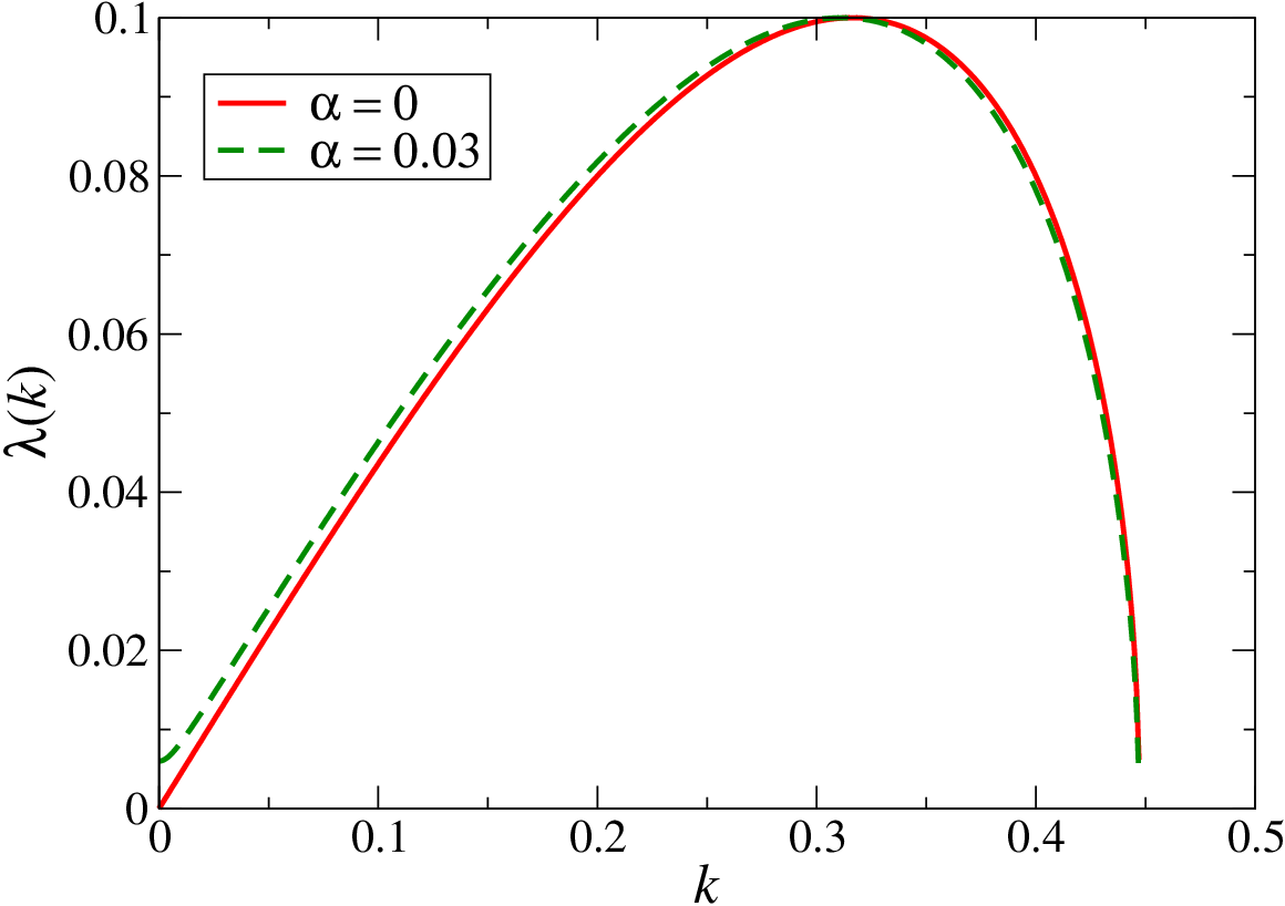
The positive real parts of Eq. (11) for and have close values, as shown in Fig. 6. This corresponds to the result that domain formation in the early stage has no remarkable difference between the damping () and no-damping () cases (See Fig. 1). From the view point of energy, the anisotropy energy does not necessarily keep decaying when . For conservation of energy, it should be also possible that both anisotropy and interfacial energies change only a little. Because of the instability of the initial state, grows, and thus, the anisotropy energy decreases.
The initial condition, which is given as spins aligned in one direction with some noises in the - plane, is the key to observe domain pattern formation in the no-damping case. Actually, if spins have totally random directions, no large domains are formed in the no-damping case, although domains are formed in damping cases () from such an initial state.
When , and , which is also one of the fixed points. Substituting into Eq. (8) and performing Fourier expansions, we have the linearized equation of ,
| (12) |
This implies that the fixed point is stable for and neutrally stable for . Although corresponds to , the same stability is expected for by symmetry.
Since the initial condition is unstable, the -component of spin grows. Moreover, linear instability is similar for and . Since are not unstable, can keep its value at around . This is why similar domain patters are formed in both damping and no-damping cases. The main difference between the two cases is that are attracting for and neutrally stable for . Since are stable and attracting in the damping case, homogeneous domains with are preferable, which leads to a smooth profile of such as Fig. 1(j). In the damping case, are neutrally stable (not attracting) fixed points, which does not necessarily make domains smooth.
V Conclusions
We have investigated the domain formation in 2D vector fields with an easy-axis anisotropy, using the LLG equation. When the initial configuration is given as almost uniform spins aligned in an in-plane direction, similar domain patterns appear in the damping () and no-damping () cases. The average domain size grows as in late times which are in a scaling regime. The damping gives no remarkable effects on domain growth and large-scale properties of domain pattern. In contrast, small-scale structures are different between the two cases, which is shown quantitatively in the structure factor. This difference is induced by the reduction of the interfacial energy due to the damping. It should be noted that the result and analysis especially in the no-damping case are valid for a limited initial condition. Although domains grow in a damping case even from spins with totally random directions, domain growth cannot occur from such a random configuration in the no-damping case.
Acknowledgements.
This work was supported by MEXT KAKENHI (No. 26103514, “Fluctuation & Structure”).References
- [1] A. Bray, Adv. Phys. 43, 357 (1994)
- [2] I. M. Lifshitz and V. V. Slyozov, J. Phys. Chem. Solids 19, 35 (1961)
- [3] C. Wagner, Z. Elektrochem 65, 581 (1961)
- [4] T. Ohta, D. Jasnow, and K. Kawasaki, Phys. Rev. Lett. 49, 1223 (1982)
- [5] D. A. Huse, Phys. Rev. B 34, 7845 (1986)
- [6] A. J. Bray, Phys. Rev. Lett. 62, 2841 (1989)
- [7] A. J. Bray, Phys. Rev. B 41, 6724 (1990)
- [8] A. J. Bray and A. D. Rutenberg, Phys. Rev. E 49, R27 (1994)
- [9] K. Kudo and Y. Kawaguchi, Phys. Rev. A 88, 013630 (2013)
- [10] J. Hofmann, S. S. Natu, and S. Das Sarma, Phys. Rev. Lett. 113, 095702 (2014)
- [11] L. A. Williamson and P. B. Blakie, Phys. Rev. Lett. 116, 025301 (2016)
- [12] H. Furukawa, Phys. Rev. A 31, 1103 (1985)
- [13] A. Lamacraft, Phys. Rev. A 77, 063622 (2008)
- [14] D. M. Stamper-Kurn and M. Ueda, Rev. Mod. Phys. 85, 1191 (2013)
- [15] Y. Kawaguchi and M. Ueda, Phys. Rep. 520, 253 (2012)
- [16] K. Kudo and Y. Kawaguchi, Phys. Rev. A 84, 043607 (2011)
- [17] M. Lakshmanan and K. Nakamura, Phys. Rev. Lett. 53, 2497 (1984)