Orthogonal AMP

Following the convention in [2], assume that $\bm{A}$ is column normalized, i.e., $\mathrm{E}\{\|\bm{A}_{:,j}\|^{2}\approx 1\}$ for each $j$. Approximate message passing (AMP) [2] refers to the following iterative process (initialized with $\bm{s}^{0}=\bm{r}_{\mathrm{Onsager}}^{0}=\mathbf{0}$)²² 2 The formulation here is different to the standard form in [2], but they can be shown to be equivalent.:

The final estimate is $\bm{s}^{t+1}$.

The use of the Onsager term is the key to AMP. It regulates correlation during iterative processing and ensures the accuracy of SE when $\bm{A}$ has IID entries [2, 3].

Define

After some manipulations, (2) can be rewritten as [3, Eqn. (3.3)] (with initialization $\bm{q}^{0}=-\bm{x}$ and $\bm{h}^{0}_{\mathrm{Onsager}}=\mathbf{0}$):

Strictly speaking, (4) is not an algorithm since it involves $\bm{x}$ that is to be estimated. Nevertheless, (4) is convenient for the analysis of AMP discussed below.

The SE for AMP refers to the following recursion:

where $Z\sim\mathcal{N}(0,1)$ is independent of $X\sim P_{X}(x)$, and $v^{2}_{0}=\mathrm{E}\{X^{2}\}$.

When $\bm{A}$ has IID Gaussian entries, SE can accurately characterize AMP, as shown in Theorem 1 [3] below.

To see the implication of Theorem 1, let $\psi(h,x)\equiv\left[\eta_{t}(x+h)-x\right]^{2}$ in (6). Then, Theorem 1 says that the empirical mean square error (MSE) of AMP defined by

converges to the predicted MSE (where $\tau_{t}$ is obtained using SE) defined by

The assumption that $\bm{A}$ contains IID entries is crucial to theorem 1. For other matrix ensembles, SE may become inaccurate. Here is an example. Consider the following function for the NLE in AMP⁴⁴ 4 Strictly speaking, $\eta_{t}$ in (9) is not a component-wise function as required in AMP. However, if Theorem 1 holds, $\sum_{j=1}^{N}\hat{\eta}_{t}^{\prime}(r_{j}^{t})/N$ will converge to a constant independent of each individual $r_{j}^{t}$. In this case, $\eta_{t}$ is an approximate component-wise function and $\sum_{j=1}^{N}{\eta}_{t}^{\prime}(r_{j}^{t})/N\approx\beta\cdot\sum_{j=1}^{N}\hat{\eta}_{t}^{\prime}(r_{j}^{t})/N$.

where $\hat{\eta}_{t}$ is the thresholding function (which is commonly used in sparse signal recovery algorithms [31]) given in (47) with $\gamma_{t}=1$. A family of $\eta_{t}$ is obtained by changing $\beta$. In particular, $\eta_{t}$ reduces to the soft-thresholding function $\hat{\eta}_{t}$ when $\beta=1$. We define a measure of the SE accuracy (after a sufficient number of iterations) as

where $MSE_{\mathrm{sim}}$ and $MSE_{\mathrm{SE}}$ are the simulated and predicted MSEs in (7) and (8). Here, as the empirical MSE is still random for large but finite $M$ and $N$, we average it over multiple realizations.

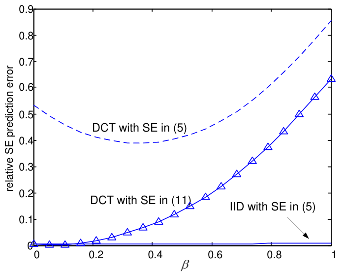
By changing $\beta$ from 0 to 1, we obtain a family of $\eta_{t}$. The solid line in Fig. 1 shows $E$ defined in (10) against $\beta$ for $\bm{A}$ being IID Gaussian. We can see that SE is quite accurate in the whole range of $\beta$ shown (with $E<10^{-2}$), which is consistent with the result in Theorem 1.

However, as shown by the dashed line, SE is not reliable when $\bm{A}$ is a partial DCT matrix. The partial DCT matrix can be obtained by uniformly randomly selecting the rows of a discrete cosine transform (DCT) matrix, and it is a widely used in compressed sensing. To see the problem, let us ignore the Onsager term. Suppose that $\bm{q}^{t}$ consists of IID entries with $\mathrm{E}\big\{(q_{j}^{t})^{2}\big\}=v_{t}^{2}$, and $\bm{q}^{t}$ is independent of $\bm{A}$ and $\bm{n}$. It can be verified that

Clearly, this is inconsistent with the SE in (5a). The problem is caused by the discrepancy in eigenvalue distributions: (11) above is derived from the eigenvalue distribution of a partial DCT matrix while (5a) from that of an IID Gaussian $\bm{A}$.

How about replacing (5a) by (11) for the partial DCT matrix? This is shown by the solid line with triangle markers in Fig. 1. We can see that $E$ is still large for $\beta>0$, which can be explained by the fact the Onsager term was ignored above. Interestingly, we can see that $E$ is very small at $\beta=0$, where the Onsager term vanishes for the related $\eta_{t}$ in (9). This observation motivates the work presented below.

Return to (1a): $\bm{y}=\bm{Ax}+\bm{n}$. Let $\bm{s}$ be an estimate of $\bm{x}$. Assume that $\bm{s}$ has IID entries with $\mathrm{E}\{(s_{j}-x_{j})^{2}\}=v^{2}$. Consider the linear estimation (LE) structure below [1] for $\bm{x}$

which is specified by $\bm{W}$. Let the singular value decomposition (SVD) of $\bm{A}$ be $\bm{A=V\Sigma U}^{\mathrm{T}}$. Throughput this paper, we will focus on the following structure for $\bm{W}$

Assume that $\bm{A}$ is unitarily-invariant. We will say that the LE (or $\bm{W}$ in (13)) is a de-correlated one if $\mathrm{tr}(\bm{I}-\bm{WA})=0$. Given an arbitrary $\hat{\bm{W}}$ that satisfies (13), we can construct $\bm{W}$ with $\mathrm{tr}(\bm{I}-\bm{WA})=0$ as follows

The following are some common examples [1] of such $\hat{\bm{W}}$

We will discuss the properties of de-correlated LE in Section III-F later.

Consider signal estimation from an observation corrupted by additive Gaussian noise

where $X\sim P_{X}(x)$ is the signal to be estimated and is independent of $Z\sim\mathcal{N}(0,1)$. For this additive Gaussian noise model, we define divergence-free estimator (or a divergence-free function of $R$) as follows.

A divergence-free function $\eta$ can be constructed as

where $\hat{\eta}$ is an arbitrary function and $C$ an arbitrary constant.

Starting with $\bm{s}^{0}=\mathbf{0}$, OAMP proceeds as

where $\bm{W}_{t}$ is de-correlated and $\eta_{t}$ is divergence-free. In the final stage, the output is

where $\eta_{t}^{{\rm{out}}}$ is not necessarily divergence-free.

OAMP is different from the standard AMP in the following aspects:

• •

  In (19a), $\bm{W}_{t}$ is restricted to be de-correlated, but it still has more choices than its counterpart $\bm{A}^{\mathrm{T}}$ in (2a)⁷⁷ 7 When the entries of $\bm{A}$ are IID with zero mean and variance $1/M$ (as considered in [2]), $N/\mathrm{tr}(\bm{A}^{\mathrm{T}}\bm{A})\approx 1$, and so $\bm{W}_{t}=\bm{A}^{\mathrm{T}}$ satisfies the condition in (13) and (14)..

• •

  In (19a), the function $\eta_{t}$ is restricted to be divergence-free. Consequently, the Onsager term vanishes.

• •

  A different estimation function $\eta_{t}^{\mathrm{out}}$ (not necessarily divergence-free) is used to produce a final estimate.

We will show that, under certain assumptions, restricting $\bm{W}_{t}$ to be de-correlated and $\eta_{t}$ to be divergence-fee ensure the orthogonality between the input and output “error” terms for both LE and NLE. The name “orthogonal AMP” comes from this fact.

Similar to (3), define the error terms as $\bm{h}^{t}\equiv\bm{r}^{t}-\bm{x}$ and $\bm{q}^{t}\equiv\bm{s}^{t}-\bm{x}$. We can write an error recursion for OAMP (similar to that for AMP in (4)) as

where $\bm{B}_{t}\equiv\bm{I}-\bm{W}_{t}\bm{A}$. Two error measures are introduced:

The SE for OAMP is defined by the following recursion

where $X\sim P_{X}(x)$ is independent of $Z\sim\mathcal{N}(0,1)$. Also, at the final stage, the MSE is predicted as

It is straightforward to verify that the SE in (23) is consistent with the error recursion in (21), provided that the following two assumptions hold for every $t$.

According to our earlier assumption below (1), $\bm{x}$ is IID and independent of $\bm{A}$ and $\bm{n}$. In OAMP, $\bm{q}^{0}=-\bm{x}$, so Assumption 2 holds for $t=-1$. Thus the two Assumptions will hold if we can prove that they imply each other in the iterative process. Unfortunately, so far, we cannot.

Assumptions 1 and 2 are only sufficient conditions for the SE. Even if they do not hold exactly, the SE may still be valid. In Section V, we will show that the SE for OAMP is accurate for a wide range of sensing matrices using simulation results. In the following two subsections, we will see that, with a de-correlated $\bm{W}_{t}$ and a divergence-free $\eta_{t}$, Assumptions 1 and 2 can partially imply each other. We emphasize that the discussions below are to provide intuitions for OAMP, which are by no means rigorous.

Eqn. (19a) performs linear estimation of $\bm{x}$ from $\bm{y}$ based on Assumption 2 (for $\bm{q}^{t}$). We first consider ensuring Assumption 1 based on Assumption 2. The independence requirements in Assumption 1 are difficult to handle. We reduce our goal to remove the correlation among the variables involved. This is achieved by restricting $\bm{W}_{t}$ to be de-correlated, as shown below.

We next consider ensuring Assumption 2 based on Assumption 1. From (21), if $\bm{q}^{t+1}$ is independent of $\bm{h}^{t}$, then it is also independent of $\bm{A}$ and $\bm{n}$, which can be seen from the Markov chain $\bm{A},\bm{n}\to\bm{h}^{t}\to\bm{q}^{t+1}$. Thus it is sufficient to ensure the independency between $\bm{q}^{t+1}$ and $\bm{h}^{t}$. Similar to the discussion in Section III-F, we reduce our goal to ensuring orthogonality between $\bm{q}^{t+1}$ and $\bm{h}^{t}$.

Suppose that Assumption 1 holds, we can construct an approximate divergence-free function $\eta_{t}$ according to (18):

All the numerical results about OAMP shown in Section V are based on (19) and (25).

There is an inherent orthogonality property associated with divergence-free functions.

If the input and output errors of the LE and NLE are independent of each other, Assumptions 1 and 2 naturally hold. However, independency is generally a tricky issue. We thus turn to orthogonality instead. The name “orthogonal AMP” came from this fact. Propositions 1 and 2 are weaker than Assumptions 1 and 2. Nevertheless, our extensive numerical study (see Section V) indicates that the SE in (23) is indeed reliable for OAMP.

Also note that each of Propositions 1 and 2 depends on one assumption, so they do not ensure orthogonality in the overall process. Nevertheless, we observed from numerical results that the orthogonality property is accurate for with unitarily-invariant matrices.

The MSEs $v_{t}^{2}\equiv\mathrm{E}\{\|\bm{q}^{t}\|^{2}\}/N$ and $\tau_{t}^{2}\equiv\mathrm{E}\{\|\bm{h}^{t}\|^{2}\}/N$ can be used as parameters of $\bm{W}_{t}$ and $\eta_{t}$. An example is the optimized $\bm{W}_{t}$ and $\eta_{t}$ given in Lemma 1 in Section IV. We now discuss empirical estimators for $v_{t}^{2}$ and $\tau_{t}^{2}$.

We can adopt the following estimator [34, Eqn. (71)] for $v_{t}^{2}$

Note that $\hat{v}_{t}^{2}$ in (30) can be negative. We may use $\max(\hat{v}_{t}^{2},\epsilon)$ as a practical estimator for $v_{t}^{2}$, where $\epsilon$ is a small positive constant. (Setting $\epsilon=0$ may cause a stability problem.)

Given $\hat{v}_{t}^{2}$, $\tau_{t}^{2}$ can be estimated using (23a):

In certain cases, Eqn. (31) can be simplified to more concise formulas. For example, (31) simplifies to $\hat{\tau}_{t}^{2}=\left({N-M}\right)/M\cdot\hat{v}_{t}^{2}+N/M^{2}\cdot{\rm{tr}}\big\{{\left({{\bm{AA}}^{\rm{T}}}\right)^{-1}}\big\}\cdot\sigma^{2}$ when $\bm{W}_{t}$ is given by the PINV estimator in (15b) together with (14). Also, simple closed-form asymptotic expression exists for (31) for certain matrix ensembles. For example, (23a) converges to (42a), (42b) and (42c) for IID Gaussian matrices with MF, PINV and LMMSE linear estimators, respectively.

The numerical results presented in Section V are obtained based on approximations in (30) and (31).

Recall that $\bm{A}=\bm{V\Sigma U}^{\mathrm{T}}$ and $\bm{B}=\bm{I-W}_{t}\bm{A}$. From (13) and (14), we have $\bm{W}_{t}=N/\mathrm{tr}(\hat{\bm{W}}_{t}\bm{A})\cdot\hat{\bm{W}}_{t}$ and $\hat{\bm{W}}_{t}=\bm{U}\hat{\bm{G}}_{t}\bm{V}^{\mathrm{T}}$. With these definitions, we can rewrite the right hand side of (23a) as follows

where $\lambda_{i}$ and $\hat{g}_{i}$ ($i=1,\ldots,M$) denote the $i$th diagonal entries of $\bm{\Sigma}$ ($M\times N$) and $\hat{\bm{G}}_{t}$ ($N\times M$), respectively. In (32), we define $\lambda_{i}=\hat{g}_{i}=0$ for $i=M+1,\ldots,N$).

In (32), $\Phi_{t}(v_{t}^{2})$ is for fixed $\{\lambda_{i}\}$ and $\{\hat{g}_{i}\}$. Now, following [35], assume that the empirical cumulative distribution function (cdf) of $\{\lambda_{1}^{2},\ldots,\lambda_{N}^{2}\}$, denoted by

converges to a limiting distribution when $M,N\to\infty$ with a fixed ratio. Furthermore, assume that $\hat{g}_{i}$ can be generated from $\lambda_{i}$ as $\hat{g}_{i}=\hat{g}_{t}(v_{t}^{2},\lambda_{i})$ with $\hat{g}_{t}$ a real-valued function. Then, (32) converges to

where the expectations (assumed to exist) are taken over the asymptotic eigenvalue distribution of $\bm{A}^{\mathrm{T}}\bm{A}$ (including the zero eigenvalues) and $\hat{g}_{t}$ stands for $\hat{g}_{t}(v_{t}^{2},\lambda)$.

We further define

where $\eta_{t}(r)\equiv C_{t}\cdot\left[\hat{\eta}_{t}(r)-\mathrm{E}\{\hat{\eta}_{t}^{\prime}(X+\tau_{t}Z)\}\cdot r\right]$ and $X$ is independent of $Z\sim\mathcal{N}(0,1)$. Then, from (32), (23b) and (35), the SE for OAMP is given by (with $v_{0}^{2}=\mathrm{E}\{X^{2}\}$)

The estimate for $\bm{x}$ in OAMP is generated by $\eta_{t}^{\mathrm{out}}$ rather than $\eta_{t}$. Thus, the MSE performance of OAMP, measured by $\|\eta_{t}^{\mathrm{out}}(\bm{r}^{t})-\bm{x}\|^{2}/N$, is predicted as

We now derive the optimal $\bm{W}_{t}$, $\eta_{t}$ and $\eta_{t}^{\mathrm{out}}$ that minimize the MSE at the final iteration.

Let $\Phi_{t}^{\star}$, $\Psi_{t}^{\star}$, and $(\Psi_{t}^{\mathrm{out}})^{\star}$ be the minimums of $\Phi_{t}$, $\Psi_{t}$, and $\Psi_{t}^{\mathrm{out}}$ respectively (the minimizations are taken over $\bm{W}_{t}$, $\eta_{t}$, and $\eta_{t}^{\mathrm{out}}$). Lemmas 1 and 2 below will be useful to prove Theorem 2.

Note that the de-correlated constraint on $\bm{W}_{t}$ and the divergence-free constraint on $\eta_{t}$ are restrictive. We next show that, provided that the SE in (36) is valid, OAMP is potentially optimal when the optimal $\bm{W}_{t}^{\star}$, $\eta_{t}^{\star}$ and $(\eta_{t}^{\mathrm{out}})^{\star}$ given in Lemma 1 are used.

We start from an IID Gaussian matrix where $A_{i,j}\sim\mathcal{N}(0,1/M)$. Fig. 2 compares simulated MSE with SE prediction for OAMP and AMP. We first assume that the entries of $\bm{x}$ are independently BPSK modulated, so $\bm{x}$ is not sparse. This is a typical detection problem in massive MIMO applications. Fig. 2 compares simulated MSEs with SE prediction for OAMP and AMP. In Fig. 2, OAMP-MF, OAMP-PINV and OAMP-LMMSE refer to, respectively, OAMP algorithms with the MF, PINV and LMMSE estimators given in (15) and the normalization in (14). The asymptotic SE formula in (34) becomes, respectively,

where $c\equiv(N-M)/M$. Comparing (42a) and (42b), we see that OAMP-PINV has better interference cancellation property than OAMP-MF (but less robust to noise). This is consistent with the observation in Fig. 2 (which represents a high SNR scenario) that OAMP-PINV can outperform OAMP-MF.

From Fig. 2, we observe good agreement between the simulated and predicted MSE for all curves. Furthermore, we see that AMP has the same convergent value as OAMP-LMMSE for IID Gaussian matrices, while the latter converges faster. Following the approach in [39], we can prove this observation but the details are omitted due to space limitation.

We next turn our attention to more general sensing matrices. Following [17], let $\bm{A}=\bm{V\Sigma U}^{\mathrm{T}}$, where $\bm{V}$ and $\bm{U}$ are independent Haar-distributed matrices (or isotropically random orthogonal matrices [32]). The nonzero singular values are set to be [17] $\lambda_{i}/\lambda_{i+1}=\kappa^{1/M}$ for $i=1,\ldots,M-1$, and $\sum_{j=1}^{M}\lambda_{i}=N$ Here, $\kappa\geq 1$ is the condition number of $\bm{A}$. We consider sparse signals, generated according to a Bernoulli-Gaussian distribution:

where $\rho\in(0,1]$ is s sparsity level and $\delta(\cdot)$ is the Dirac delta function.

Fig. 3 shows the simulated and predicted MSEs for OAMP for the above ill-conditioned sensing matrix. The SE of OAMP is based on the empirical form in (32) as $\{\lambda_{i}\}$ are fixed in this example. We can make the following observations.

• •

  The performances of AMP and OAMP-MF deteriorate in this case. The SE prediction for AMP is not shown in Fig. 3 since it is noticeably different from the simulation result. (See Fig. 1 for a similar issue.)

• •

  The performance of OAMP is strongly affected by the LE structure. OAMP-PINV and OAMP-LMMSE significantly outperform OAMP-MF.

• •

  The most interesting point is that the SE in (36) can accurately predict the OAMP simulation results for all the LE structures in Fig. 3. We observed in simulations that such good agreement also holds for LEs beyond the three options shown in Fig. 3.

Fig. 4 compares the MSE performances of AMP, OAMP and genie-aided MMSE (where the positions of the non-zero entries are known) as the condition number of $\bm{A}$ varies. AMP with adaptive damping (AMP-damping) [17] (based on the Matlab code released by its authors⁸⁸ 8 Available at http://sourceforge.net/projects/gampmatlab/ and the parameters used in [17, Fig. 1]) and GAMP-ADMM [19] are also shown. From Fig. 4, we can see that the performance of OAMP-LMMSE is significantly better than those of AMP, AMP-damping and ADMM-GAMP for highly ill-conditioned scenarios. (ADMM-GAMP slightly outperforms OAMP-LMMSE for $\kappa\leq 100$ since the former involves more iterations in this example.) OAMP-PINV has worse performance than AMP when $\kappa\geq 10$ but performs reasonably well for large $\kappa$. OAMP-MF does not work well and thus not included.

For the schemes shown in Fig. 4, AMP have the lowest complexity. OAMP-PINV requires one additional matrix inversion, but it can be pre-computed as it remains unchanged during the iterations. Both OAMP-LMMSE and ADMM-GAMP require matrix inversions in each iteration. As pointed out in [19], it may be possible to replace the matrix inversion in ADMM-GAMP using an iterative method such as conjugate gradient [40]. Similar approximation should be possible for OAMP as well.

In the examples used above, matrix inversion is involved for $\hat{\bm{W}}^{\mathrm{PINV}}$ and $\hat{\bm{W}}^{\mathrm{LMMSE}}$ in (15b) and (15c), so their complexity per iteration can be higher than that of AMP. (Note that the overall complexity also depends on the convergence speed, for which AMP and OAMP behave differently as seen in Fig.  4.) In the following, we will consider partial orthogonal matrices characterized by $\bm{AA}^{\mathrm{T}}=N/M\cdot\bm{I}$ (here $N/M$ is a normalization constant). Then inversion operation is not necessary. For example, in this case $\hat{\bm{W}}^{\mathrm{LMMSE}}$ is given by

References

- [1] S. M. Kay, Fundamentals of statistical signal processing: estimation theory. NJ: Prentice-Hall PTR, 1993.
- [2] D. L. Donoho, A. Maleki, and A. Montanari, “Message-passing algorithms for compressed sensing,” in Proc. Nat. Acad. Sci., vol. 106, no. 45, Nov. 2009.
- [3] M. Bayati and A. Montanari, “The dynamics of message passing on dense graphs, with applications to compressed sensing,” IEEE Trans. Inf. Theory, vol. 57, no. 2, pp. 764–785, Feb. 2011.
- [4] M. Bayati, M. Lelarge, A. Montanari et al., “Universality in polytope phase transitions and message passing algorithms,” The Annals of Applied Probability, vol. 25, no. 2, pp. 753–822, 2015.
- [5] T. Richardson and R. Urbanke, “The capacity of low-density parity-check codes under message-passing decoding,” IEEE Trans. Inf. Theory, vol. 47, no. 2, pp. 599–618, Feb. 2001.
- [6] S. ten Brink, “Convergence behavior of iteratively decoded parallel concatenated codes,” IEEE Trans. Inf. Theory, vol. 49, no. 10, pp. 1727–1737, Oct 2001.
- [7] D. Donoho, A. Maleki, and A. Montanari, “Message passing algorithms for compressed sensing: I. motivation and construction,” in Information Theory (ITW 2010, Cairo), 2010 IEEE Information Theory Workshop on, Jan 2010, pp. 1–5.
- [8] D. Guo and S. Verdu, “Randomly spread CDMA: asymptotics via statistical physics,” IEEE Trans. Inf. Theory, vol. 51, no. 6, pp. 1983–2010, Jun. 2005.
- [9] S. Rangan, V. Goyal, and A. K. Fletcher, “Asymptotic analysis of MAP estimation via the replica method and compressed sensing,” in Advances in Neural Information Processing Systems, 2009, pp. 1545–1553.
- [10] A. Tulino, G. Caire, S. Verdu, and S. Shamai, “Support recovery with sparsely sampled free random matrices,” IEEE Trans. Inf. Theory, vol. 59, no. 7, pp. 4243–4271, Jul. 2013.
- [11] C.-K. Wen and K.-K. Wong, “Analysis of compressed sensing with spatially-coupled orthogonal matrices,” arXiv preprint arXiv:1402.3215, 2014.
- [12] S. Wu, L. Kuang, Z. Ni, J. Lu, D. Huang, and Q. Guo, “Low-complexity iterative detection for large-scale multiuser MIMO-OFDM systems using approximate message passing,” IEEE J. Sel. Topics Signal Process., vol. 8, no. 5, pp. 902–915, Oct 2014.
- [13] C. Jeon, R. Ghods, A. Maleki, and C. Studer, “Optimality of large MIMO detection via approximate message passing,” in Proc. IEEE Int. Symp. Inf. Theory (ISIT), June 2015, pp. 1227–1231.
- [14] C.-K. Wen, S. Jin, K.-K. Wong, C.-J. Wang, and G. Wu, “Joint channel and data estimation for large-MIMO systems with low-precision ADCs,” in Proc. IEEE Int. Symp. Inf. Theory (ISIT), June 2015, pp. 1237–1241.
- [15] C. Rush, A. Greig, and R. Venkataramanan, “Capacity-achieving sparse regression codes via approximate message passing decoding,” in Proc. IEEE Int. Symp. Inf. Theory (ISIT), June 2015, pp. 2016–2020.
- [16] J. Barbier and F. Krzakala, “Approximate message-passing decoder and capacity-achieving sparse superposition codes,” arXiv preprint arXiv:1503.08040, 2015.
- [17] J. Vila, P. Schniter, S. Rangan, F. Krzakala, and L. Zdeborová, “Adaptive damping and mean removal for the generalized approximate message passing algorithm,” in Acoustics, Speech and Signal Processing (ICASSP), 2015 IEEE International Conference on, 2015, pp. 2021–2025.
- [18] A. Manoel, F. Krzakala, E. W. Tramel, and L. Zdeborová, “Sparse estimation with the swept approximated message-passing algorithm,” arXiv preprint arXiv:1406.4311, 2014.
- [19] S. Rangan, A. K. Fletcher, P. Schniter, and U. Kamilov, “Inference for generalized linear models via alternating directions and Bethe free energy minimization,” arXiv preprint arXiv:1501.01797, 2015.
- [20] Y. Kabashima and M. Vehkapera, “Signal recovery using expectation consistent approximation for linear observations,” in Proc. IEEE Int. Symp. Inf. Theory (ISIT), Jun. 2014, pp. 226–230.
- [21] B. Cakmak, O. Winther, and B. Fleury, “S-AMP: Approximate message passing for general matrix ensembles,” in Information Theory Workshop (ITW), 2014 IEEE, Nov. 2014, pp. 192–196.
- [22] Q. Guo and J. Xi, “Approximate message passing with unitary transformation,” arXiv preprint arXiv:1504.04799, 2015.
- [23] B. Çakmak, M. Opper, B. H. Fleury, and O. Winther, “Self-averaging expectation propagation,” arXiv preprint arXiv:1608.06602, 2016.
- [24] M. Opper, B. Cakmak, and O. Winther, “A theory of solving TAP equations for ising models with general invariant random matrices,” Journal of Physics A: Mathematical and Theoretical, vol. 49, no. 11, p. 114002, 2016.
- [25] E. Bostan, M. Unser, and J. P. Ward, “Divergence-free wavelet frames,” IEEE Signal Process. Lett., vol. 22, no. 8, pp. 1142–1146, 2015.
- [26] X. Yuan, J. Ma, and L. Ping, “Energy-spreading-transform based MIMO systems: Iterative equalization, evolution analysis, and precoder optimization,” IEEE Trans. Wireless Commun., vol. 13, no. 9, pp. 5237–5250, Sept. 2014.
- [27] J. Ma, X. Yuan, and L. Ping, “Turbo compressed sensing with partial DFT sensing matrix,” IEEE Signal Process. Lett., vol. 22, no. 2, pp. 158–161, Feb. 2015.
- [28] J. Ma and L. Ping, “Orthogonal AMP,” arXiv preprint arXiv:1602.06509, 2016.
- [29] S. Rangan, P. Schniter, and A. Fletcher, “Vector approximate message passing,” arXiv preprint arXiv:1610.03082, 2016.
- [30] J. Ma and L. Ping, “Orthogonal AMP for compressed sensing with unitarily-invariant matrices,” in 2016 IEEE Information Theory Workshop (ITW), Sept 2016, pp. 280–284.
- [31] D. Donoho, “De-noising by soft-thresholding,” IEEE Trans. Inf. Theory, vol. 41, no. 3, pp. 613–627, May 1995.
- [32] A. M. Tulino and S. Verdú, Random matrix theory and wireless communications. Now Publishers Inc, 2004, vol. 1.
- [33] C. Stein, “A bound for the error in the normal approximation to the distribution,” in Proc. 6th Berkeley Symp. Math. Statist. Probab., 1972.
- [34] J. Vila and P. Schniter, “Expectation-maximization Gaussian-mixture approximate message passing,” IEEE Trans. Signal Process., vol. 61, no. 19, pp. 4658–4672, Oct. 2013.
- [35] M. Vehkapera, Y. Kabashima, and S. Chatterjee, “Analysis of regularized LS reconstruction and random matrix ensembles in compressed sensing,” in Proc. IEEE Int. Symp. Inf. Theory (ISIT), Jun. 2014, pp. 3185–3189.
- [36] D. Guo, Y. Wu, S. Shamai, and S. Verdu, “Estimation in Gaussian noise: properties of the minimum mean-square error,” IEEE Trans. Inf. Theory, vol. 57, no. 4, pp. 2371–2385, Apr. 2011.
- [37] C. Guo and M. E. Davies, “Near optimal compressed sensing without priors: parametric SURE approximate message passing,” IEEE Trans. Signal Process., vol. 63, no. 8, pp. 2130–2141, 2015.
- [38] Z. Xue, J. Ma, and X. Yuan, “D-OAMP: A denoising-based signal recovery algorithm for compressed sensing,” arXiv preprint arXiv:1610.05991, 2016.
- [39] J. Ma, X. Yuan, and L. Ping, “On the performance of turbo signal recovery with partial DFT sensing matrices,” IEEE Signal Process. Lett., vol. 22, no. 10, pp. 1580–1584, Oct 2015.
- [40] H. A. Van der Vorst, Iterative Krylov methods for large linear systems. Cambridge University Press, 2003, vol. 13.
- [41] M. Lustig, D. L. Donoho, J. M. Santos, and J. M. Pauly, “Compressed sensing MRI,” IEEE Signal Process. Mag., vol. 25, no. 2, pp. 72–82, March 2008.
- [42] D. Donoho, I. Johnstone, and A. Montanari, “Accurate prediction of phase transitions in compressed sensing via a connection to minimax denoising,” IEEE Trans. Inf. Theory, vol. 59, no. 6, pp. 3396–3433, June 2013.
- [43] F. Hiai and D. Petz, Asymptotic freeness almost everywhere for random matrices. University of Aarhus. Centre for Mathematical Physics and Stochastics (MaPhySto)[MPS], 1999.
- [44] S. Rangan. Generalized approximate message passing for estimation with random linear mixing. Preprint, 2010. [Online]. Available: http://arxiv.org/abs/1010.5141.