Frozen Gaussian approximation with surface hopping for mixed quantum-classical dynamics: A mathematical justification of fewest switches surface hopping algorithmsThanks: This work is partially supported by the National Science Foundation under grants DMS-1312659, DMS-1454939 and RNMS11-07444 (KI-Net). J.L. is also partially supported by the Alfred P. Sloan Foundation. J.L. would like to thank Sara Bonella, Giovanni Ciccotti, Joe Subotnik and Jonathan Weare for helpful discussions, and especially John Tully for encouragement.

Jianfeng Lu Address: Department of Mathematics, Department of Physics, and Department of Chemistry, Duke University, Box 90320, Durham NC 27708, USA Email address: jianfeng@math.duke.edu and Zhennan Zhou Address: Department of Mathematics, Duke University, Box 90320, Durham NC 27708, USA Email address: zhennan@math.duke.edu

Date: August 24, 2026

Abstract.

We develop a surface hopping algorithm based on frozen Gaussian approximation for semiclassical matrix Schrödinger equations, in the spirit of Tully’s fewest switches surface hopping method. The algorithm is asymptotically derived from the Schrödinger equation with rigorous approximation error analysis. The resulting algorithm can be viewed as a path integral stochastic representation of the semiclassical matrix Schrödinger equations. Our results provide mathematical understanding to and shed new light on the important class of surface hopping methods in theoretical and computational chemistry.

1. Introduction

The surface hopping algorithms, in particular the celebrated Tully’s fewest switches surface hopping (FSSH) algorithm [30, 7], are widely used in theoretical and computational chemistry for mixed quantum-classical dynamics in the non-adiabatic regime.

The Schrödinger equation, which is often high dimensional in chemistry applications, is impractical to solve directly due to curse of dimensionality. Thus, development of algorithms based on semiclassical approximation, which only involve solving ODEs, is necessary. Within the Born-Oppenheimer approximation, the resulting algorithm from the semiclassical approximation is the familiar ab initio molecular dynamics and related semiclassical algorithms. However, in many applications, the adiabatic assumption in the Born-Oppenheimer approximation is violated, thus, we need to consider the non-adiabatic dynamics. The surface hopping algorithms are hence proposed to incorporate in quantum behavior due to the non-adiabaticity.

Despite the huge popularity of the algorithm and the many attempts in the chemistry literature for corrections and further improvements (see e.g., [24, 11, 2, 27, 19, 26, 8]), which is a very active area to date, the understanding of such algorithms, in particular, how surface hopping type algorithms can be derived from the nuclei Schrödinger equations, remains rather poor.

In this work, we rigorously derive a surface hopping algorithm, named frozen Gaussian approximation with surface hopping (FGA-SH), to approximate the Schrödinger equations with multiple adiabatic states in the semiclassical regime. The FGA-SH algorithm shares similar spirit as the FSSH algorithms used in the chemistry literature [30], while it also differs in some essential ways. Hence, besides providing a rigorously asymptotically correct approximation, our derivation hopefully will also help clarify several issues and mysteries around the FSSH algorithm, and lead to systematic improvement of this type of algorithms.

The key observation behind our work is a path integral stochastic representation to the solution to the semiclassical Schrödinger equations. The surface hopping algorithm can be in fact viewed as a direct Monte Carlo method for evaluating the path integral. Thus, the path space average provides an approximation to the solution of a high dimensional PDE, similar to the familiar Feynman-Kac formula for reaction diffusion type equations. To the best of our knowledge, this has not been observed in the literature, and it is crucial for understanding what the surface hopping algorithm really tries to compute.

In this stochastic representation, the path space consists of continuous trajectory in the phase space, whose evolution switches between classical Hamiltonian flows corresponding to each energy surface, and is hence piecewise deterministic, except at hoppings. This is why these algorithms are called surface hopping algorithms. Also to avoid any potential confusion, while we approximate solutions to the Schrödinger equation, the path integral we consider here (as it only works in the semiclassical limit) is very different from the usual Feynman path integral for quantum mechanics. In particular, the stochastic representation is well defined and gives an accurate approximation to the solution of the Schrödinger equation in the semiclassical regime.

Before we continue, let us review some related mathematical works. Somehow rather confusingly, sometimes the term “surface hopping” is used for a very different algorithm [29] which is based on Landau-Zener transition asymptotics [18, 34]. This algorithm is designed for the situation of a single avoided crossing, while the type of surface hopping algorithm we consider in this paper, which is mostly often used in chemistry today, is quite different and aims to work for general situations. The Landau-Zener asymptotics has been mathematically studied by Hagedorn and Joye [6, 5]. The algorithm based on Landau-Zener formula is also studied in the mathematics literature, see e.g., [20, 4, 13]. While the algorithm we consider is very different, some of these numerical techniques might be used in our context as well.

For the surface hopping algorithm we studied in this work, the understanding in the chemistry literature (see e.g., [8, 11, 26]) often starts from the quantum-classical Liouville equation [15], which is a natural generalization of the usual Moyal’s evolution equation of Wigner distribution to the matrix Schrödinger equations. In the mathematics literature, the quantum-classical Liouville equation was studied numerically in [3] in low dimensions very recently. While we are able to derive a surface hopping type algorithm, our derivation is based on a different tool for semiclassical analysis, the frozen Gaussian approximation, aka the Herman-Kluk propagator [10, 16, 17, 28, 22, 21]. It is not yet clear to us whether the surface hopping algorithms used in the chemistry literature (and the one we derived) can be rigorously justified from the view point of quantum-classical Liouville equation. This remains an interesting research direction.

The surface hopping algorithm we derive is based on asymptotic analysis on the phase space. The ansatz of the solution, represented as an integration over the phase space and possible configurations of hopping times is given in Section 2, after a brief review of the frozen Gaussian approximation for single surface case. For the algorithmic purpose, it is more useful to take a stochastic representation of the ansatz as a path integral, which is given in Section 3. A simple Monte Carlo algorithm for the path space average then leads to a rigorously justifiable surface hopping algorithm, which we will compare with and connect to those used in the chemistry literature in Section 3.3. The asymptotic derivation of the ansatz is given in Section 4. The main rigorous approximation result is stated in Section 5, together with a few illustrating examples. Some numerical examples of the algorithm are discussed in Section 6. We conclude the paper with proofs of the main result in Section 7.

2. Integral representation for semiclassical matrix Schrödinger equations

2.1. Two-state matrix Schrödinger equation

Consider the rescaled Schrödinger equation for nuclei and electrons

(2.1)

i\varepsilon\frac{\partial}{\partial t}u=-\frac{\varepsilon^{2}}{2}\Delta_{x}u-\frac{1}{2}\Delta_{r}u+V(x,r)u.

where $u(t,x,r)$ is the total wave function, $x\in{\mathbb{R}}^{m}$ represents the nuclear degrees of freedom, $r\in{\mathbb{R}}^{n}$ denotes the electronic degrees of freedom, and $V(x,r)$ is the total interaction potential. Here, $\varepsilon\ll 1$ is the square root of the mass ratio between the electrons and the nuclei (for simplicity, we assume that all nuclei have the same mass).

We define the electronic Hamiltonian

H_{e}=-\frac{1}{2}\Delta_{r}+V(x,r),

whose eigenstates $\Psi_{k}(r;x)$ , given by

(2.2)

H_{e}\Psi_{k}(r;x)=E_{k}(x)\Psi_{k}(r;x),

are called the adiabatic states. Note that in the eigenvalue problem (2.2), $x$ enters as a parameter. In particular, viewed as a function of $x$ , the eigenvalues $E_{k}(x)$ will be referred as energy surfaces.

In this work, we will only consider a finite number of adiabatic states, that is, we assume the following expansion of the total wave function

u(t,x,r)=\sum_{n=0}^{N-1}u_{n}(t,x)\Psi_{n}(r;x).

This is justified if the rest of the spectrum of $H_{e}$ is far separated from that of the states under consideration, so that the transition between these $N$ energy surfaces and others is negligible. For the separation condition and the corresponding spectral gap assumption, the readers may refer to [25, 23] for detailed discussions.

In fact, for simplicity of notation, we will assume that the number of states is $N=2$ , the extension to any finite $N$ is straightforward. In this case, $u(t,x,r)=u_{0}(t,x)\Psi_{0}(r;x)+u_{1}(t,x)\Psi_{1}(r;x)$ , the original equation is equivalent to a system of PDEs of $U=\bigl(\begin{smallmatrix}u_{0}\\ u_{1}\end{smallmatrix}\bigr)$ , which we will henceforth refer to as the matrix Schrödinger equation:

(2.3)

i\varepsilon\partial_{t}\begin{pmatrix}u_{0}\\ u_{1}\end{pmatrix}=-\frac{\varepsilon^{2}}{2}\Delta_{x}\begin{pmatrix}u_{0}\\ u_{1}\end{pmatrix}+\begin{pmatrix}E_{0}\\ &E_{1}\end{pmatrix}\begin{pmatrix}u_{0}\\ u_{1}\end{pmatrix}-\frac{\varepsilon^{2}}{2}\begin{pmatrix}D_{00}&{D_{01}}\\ {D_{10}}&D_{11}\end{pmatrix}\begin{pmatrix}u_{0}\\ u_{1}\end{pmatrix}-\varepsilon^{2}\sum_{j=1}^{m}\begin{pmatrix}d_{00}&{d_{01}}\\ {d_{10}}&d_{11}\end{pmatrix}_{j}\partial_{x_{j}}\begin{pmatrix}u_{0}\\ u_{1}\end{pmatrix},

where

D_{kl}(x)=\langle\Psi_{k}(r;x),\Delta_{x}\Psi_{l}(r;x)\rangle_{r},\quad\left(d_{kl}(x)\right)_{j}=\langle\Psi_{k}(r;x),\partial_{x_{j}}\Psi_{l}(r;x)\rangle_{r},\quad\text{for }k,l=0,1,\;j=1,\ldots,m.

2.2. Brief review of the frozen Gaussian approximation

Before we consider the matrix Schrödinger equation (2.3), let us recall the ansatz of frozen Gaussian approximation (aka Herman-Kluk propagator) [10, 16, 17, 28] for scalar Schrödinger equation

(2.4)

i\varepsilon\frac{\partial}{\partial t}u(t,x)=-\frac{\varepsilon^{2}}{2}\Delta u(t,x)+E(x)u(t,x).

Note that if we drop the terms depending on $d$ and $D$ in (2.3), it decouples to two equations of the form of (2.4). The algorithm that we will derive for (2.3) can be viewed as an extension of the FGA to the matrix Schrödinger equation.

The frozen Gaussian approximation is a convergent approximation to the solution of (2.4) with $\mathcal{O}(\varepsilon)$ error [28]. It is based on the following integral representation of an approximate solution to (2.4)

(2.5)

u_{\text{FGA}}(t,x)=\frac{1}{(2\pi\varepsilon)^{3m/2}}\int_{{\mathbb{R}}^{3m}}a(t,q,p)e^{\frac{i}{\varepsilon}\Phi(t,x,y,q,p)}u(0,y)\,\mathrm{d}y\,\mathrm{d}q\,\mathrm{d}p,

where $u(0,\cdot)$ is the initial condition. Here, the phase function $\Phi$ is given by

\Phi(t,x,y,q,p)=S(t,q,p)+P(t,q,p)\cdot(x-Q(t,q,p))-p\cdot(y-q)+\frac{i}{2}|x-Q(t,q,p)|^{2}+\frac{i}{2}|y-q|^{2}.

Given $q$ and $p$ as parameters, the evolution of $Q$ and $P$ are governed by the Hamiltonian flow according to classical Hamiltonian $h(q,p)=\frac{1}{2}\lvert p\rvert^{2}+E(q)$ ,

	$\displaystyle\frac{\,\mathrm{d}}{\,\mathrm{d}t}Q$	$\displaystyle=\partial_{p}h(Q,P),$
	$\displaystyle\frac{\,\mathrm{d}}{\,\mathrm{d}t}P$	$\displaystyle=-\partial_{q}h(Q,P),$

with initial conditions $Q(0,p,q)=q$ and $P(0,q,p)=p$ . The solution to the Hamiltonian equations defines a trajectory on the phase space ${\mathbb{R}}^{2m}$ , which we call FGA trajectory. $S$ is the action corresponding to the Hamiltonian flow, with initial condition $S(0,q,p)=0$ . The equation of $a$ is obtained by matched asymptotics and is given by:

(2.6)

\frac{\,\mathrm{d}}{\,\mathrm{d}t}a=\frac{1}{2}a\tr\bigl(Z^{-1}\bigl(\partial_{z}P-i\partial_{z}Q\nabla^{2}_{Q}E(Q)\bigr)\bigr)

with initial condition $a(0,q,p)=2^{m/2}$ , where we have used the short hand notations

\partial_{z}=\partial_{q}-i\partial_{p},\quad\text{and}\quad Z=\partial_{z}(Q+iP).

Equivalently, we can rewrite as

u_{\text{FGA}}(t,x)=\frac{1}{(2\pi\varepsilon)^{3m/2}}\int_{{\mathbb{R}}^{2m}}A(t,q,p)e^{\frac{i}{\varepsilon}\Theta(t,x,q,p)}\,\mathrm{d}q\,\mathrm{d}p,

where

	$\displaystyle\Theta(t,x,q,p)$	$\displaystyle=S(t,q,p)+P(t,q,p)\cdot(x-Q(t,q,p))+\frac{i}{2}\|x-Q(t,q,p)\|^{2},$
	$\displaystyle A(t,q,p)$	$\displaystyle=a(t,q,p)\int_{{\mathbb{R}}^{m}}u_{0}(y)e^{\frac{i}{\varepsilon}(-p\cdot(y-q)+\frac{i}{2}\|y-q\|^{2})}\,\mathrm{d}y.$

As $A$ only differs from $a$ by a constant multiplication factor, it satisfies the same equation as $a$ does (with different initial condition).

The following lemma, which we directly quote from [21]*Lemma 3.1, states that the FGA ansatz reproduces the initial condition.

Lemma 2.1.

For $u\in L^{2}({\mathbb{R}}^{m})$ , we have

u(x)=\frac{1}{(2\pi\varepsilon)^{3m/2}}\int_{{\mathbb{R}}^{3m}}2^{\frac{m}{2}}e^{\frac{i}{\varepsilon}\Phi(0,x,y,q,p)}u(y)\,\mathrm{d}y\,\mathrm{d}q\,\mathrm{d}p.

The next lemma is crucial for the asymptotic matching to derive the evolution equations. The proof can be found in [21]*Lemma 3.2 and [22]*Lemma 5.2. We recall this lemma here as it will be used in the extension of frozen Gaussian approximation to the matrix Schrödinger equations.

Lemma 2.2.

For any vector $b(y,q,p)$ and any matrix $M(y,q,p)$ in Schwartz class viewed as functions of $(y,q,p)$ , we have

b\cdot(x-Q)\sim-\varepsilon\partial_{z_{k}}(b_{j}Z_{jk}^{-1}),

and

(x-Q)\cdot M(x-Q)\sim\varepsilon\partial_{z_{l}}Q_{j}M_{jk}Z_{kl}^{-1}+\mathcal{O}(\varepsilon^{2})

where Einstein’s summation convention has been assumed. Moreover, for multi-index $\alpha$ that $|\alpha|\geqslant 3$ ,

(x-Q)^{\alpha}\sim\mathcal{O}(\varepsilon^{|\alpha|-1}).

Here, we denote by $f\sim g$ that

\int_{{\mathbb{R}}^{3m}}fe^{\frac{i}{\varepsilon}\Phi}\,\mathrm{d}y\,\mathrm{d}q\,\mathrm{d}p=\int_{{\mathbb{R}}^{3m}}ge^{\frac{i}{\varepsilon}\Phi}\,\mathrm{d}y\,\mathrm{d}q\,\mathrm{d}p.

2.3. The integral representation for surface hopping

We now consider extending the integral representation in the previous subsection to the matrix Schrödinger equation by incorporating the coupling of the two energy surfaces, which is the basis of the FGA-SH algorithm.

Let us assume, for simplicity of notation, that the initial condition concentrates on energy surface $E_{0}$ (i.e., $u_{1}(0,x)=0$ and $u_{0}$ is non-zero). The extension to general initial condition is straightforward as the equation is linear. We construct an approximation to the total wave function following the ansatz below. We will prove rigorously that it gives an $\mathcal{O}(\varepsilon)$ approximation to the true solution; see the convergence statement in Section 5. The integral representation here is fully deterministic, and our FGA-SH algorithm can be understood as a Monte Carlo algorithm for evaluation.

(2.7)

u_{\text{FGA}}(t,x,r)=K^{(0)}_{00}(t,x,r)+K^{(1)}_{01}(t,x,r)+K^{(2)}_{00}(t,x,r)+K^{(3)}_{01}(t,x,r)+\cdots

where,

(2.8)

K^{(l)}_{mn}(t,x,r)=\Psi_{n}(r;x)u_{m}^{(l)}(t,x)

represents the contribution to the ansatz by wave packets initiated at surface $m$ , ends at surface $n$ , and switches the propagating surface $l$ times in between — the meaning of which will become clear below. Thus, we can rewrite (2.7) as

u_{\text{FGA}}(t,x,r)=\Psi_{0}(r;x)\left(u_{0}^{(0)}(t,x)+u_{0}^{(2)}(t,x)+\cdots\right)+\Psi_{1}(r;x)\left(u_{0}^{(1)}(t,x)+u_{0}^{(3)}(t,x)+\cdots\right).

We will refer this as the surface hopping ansatz. The idea of splitting the wave function in this way is similar to that used in the work by Wu and Herman [31, 32, 33], which is also based on the frozen Gaussian approximation. The two approaches are different however in several essential ways, as we will explain in §3.3.

As we consider initial condition starting from the surface $0$ , for simplicity of notation, we will drop the subscripts $0$ in $u_{0}^{(n)}$ for now. In the ansatz, $u^{(0)}$ consists of contribution from wave packets propagating only on energy surface $E_{0}$ , without switching to $E_{1}$ surface. It is given by the ansatz of frozen Gaussian approximation on a single surface as in Section 2.2:

(2.9)

u^{(0)}(t,x)=\frac{1}{(2\pi\varepsilon)^{3m/2}}\int A^{(0)}(t,z_{0})\exp\left(\frac{i}{\varepsilon}\Theta^{(0)}(t,z_{0},x)\right)\,\mathrm{d}z_{0},

where we have used $z_{0}=(q_{0},p_{0})$ to denote phase space variables,

\Theta^{(0)}(t,q,p,x)=S^{(0)}(t,q,p)+P^{(0)}(t,q,p)\cdot\left(x-Q^{(0)}(t,q,p)\right)+\frac{i}{2}\left|x-Q^{(0)}(t,q,p)\right|^{2},

and

(2.10)

A^{(0)}(t,q,p)=a^{(0)}(t,q,p)\int_{{\mathbb{R}}^{m}}u_{0}(y)e^{\frac{i}{\varepsilon}(-p\cdot(y-q)+\frac{i}{2}|y-q|^{2})}\,\mathrm{d}y.

Here, the evolution of the quantities $S^{(0)}$ , $P^{(0)}$ , $Q^{(0)}$ and $A^{(0)}$ are determined by matched asymptotic and will be specified below. We will refer these quantities as FGA variables in the sequel.

For $n>0$ , the wave function $u^{(n)}$ counts for contribution of wave packets that switch between the two energy surfaces $n$ times. Given $n$ , to specify the integral representation, let us denote $T_{n:1}=(t_{n},\cdots,t_{1})$ a sequence of times ordered backwardly, i.e., they satisfy

0\leqslant t_{1}\leqslant t_{2}\leqslant\cdots\leqslant t_{n}\leqslant t.

The ansatz for $u^{(n)}$ is given by

(2.11)

u^{(n)}(t,x)=\frac{1}{(2\pi\varepsilon)^{3m/2}}\int\,\mathrm{d}z_{0}\int_{0}^{t}\,\mathrm{d}t_{n}\int_{0}^{t_{n}}\,\mathrm{d}t_{n-1}\cdots\int_{0}^{t_{2}}\,\mathrm{d}t_{1}\;\tau^{(1)}(T_{1:1},z_{0})\cdots\tau^{(n)}(T_{n:1},z_{0})\times\\ \times A^{(n)}(t,T_{n:1},z_{0})\exp\left(\frac{i}{\varepsilon}\Theta^{(n)}(t,T_{n:1},z_{0},x)\right)

where

\Theta^{(n)}(t,T_{n:1},z_{0},x)=S^{(n)}(t,T_{n:1},z_{0})+P^{(n)}(t,T_{n:1},z_{0})\cdot\left(x-Q^{(n)}(t,T_{n:1},z_{0})\right)+\frac{i}{2}\left|x-Q^{(n)}(t,T_{n:1},z_{0})\right|^{2},

and

A^{(n)}(t,T_{n:1},z_{0})=a^{(n)}(t,T_{n:1},z_{0})\int_{{\mathbb{R}}^{m}}u_{0}(y)e^{\frac{i}{\varepsilon}(-p\cdot(y-q)+\frac{i}{2}|y-q|^{2})}\,\mathrm{d}y.

To simplify the notation, we will often write (2.11) as

(2.12)

u^{(n)}(t,x)=\frac{1}{(2\pi\varepsilon)^{3m/2}}\int\,\mathrm{d}z_{0}\int_{0\leqslant t_{1}\leqslant\cdots\leqslant t_{n}\leqslant t}\tau^{(1)}\cdots\tau^{(n)}\;A^{(n)}\;\exp\left(\frac{i}{\varepsilon}\Theta^{(n)}\right)\,\mathrm{d}T_{n:1},

where $\,\mathrm{d}T_{n:1}=\,\mathrm{d}t_{1}\cdots\,\mathrm{d}t_{n}$ . Note that in (2.11), we integrate over all possible sequences of $n$ ordered times in the time interval $[0,t]$ .

Note that given the time sequence $T_{n:1}$ , (2.11) depends on the FGA variables $S^{(n)},P^{(n)},Q^{(n)},A^{(n)}$ , and also $\tau^{(k)}$ for $k=1,\ldots,n$ . We will refer $\tau^{(k)}$ as the hopping coefficients, since they are related to the jumping intensity of our stochastic algorithm. Note that as other FGA variables, $\tau^{(k)}(T_{k:1},z_{0})$ depend on the time sequence $T_{k:1}$ and $z_{0}$ .

Let us now specify the evolution equations for the FGA variables and hopping coefficients involved in (2.9) and (2.11) to complete the integral representation. The asymptotic derivation of these equations will be given in Section 4.

Recall that for $n=0$ , the FGA trajectory evolves on a single energy surface $E_{0}$ . For $n>0$ , the trajectory will switch between the two surfaces at given time sequences $T_{n:1}$ . More precisely, $T_{n:1}=(t_{n},t_{n-1},\ldots,t_{1})$ determines a partition of the time interval $[0,t]$ . Each FGA variable evolves piecewisely in time on alternating energy surfaces, starting on energy surface $0$ (due to our assumption of the initial condition). For convenience, we take the convention $t_{0}=0$ and $t_{n+1}=t$ in the following.

When $t\in[t_{k},t_{k+1})$ for $k$ being an even integer, all the FGA variables evolve on energy surface $l^{(k)}=0$ , and for $k$ odd, the trajectory evolves on energy surface $l^{(k)}=1$ . The evolution equations are given accordingly as


(2.13a)	$\displaystyle\frac{\,\mathrm{d}}{\,\mathrm{d}t}Q^{(k)}$	$\displaystyle=P^{(k)},$
(2.13b)	$\displaystyle\frac{\,\mathrm{d}}{\,\mathrm{d}t}P^{(k)}$	$\displaystyle=-\nabla E_{l^{(k)}}(Q^{(k)}),$
(2.13c)	$\displaystyle\frac{\,\mathrm{d}}{\,\mathrm{d}t}S^{(k)}$	$\displaystyle=\frac{1}{2}(P^{(k)})^{2}-E_{l^{(k)}}(Q^{(k)}),$
(2.13d)	$\displaystyle\frac{\,\mathrm{d}}{\,\mathrm{d}t}A^{(k)}$	$\displaystyle=\frac{1}{2}A^{(k)}\tr\left((Z^{(k)})^{-1}\left(\partial_{z}P^{(k)}-i\partial_{z}Q^{(k)}\nabla^{2}_{Q}E_{l^{(k)}}(Q^{(k)})\right)\right)-A^{(k)}d_{l^{(k)}l^{(k)}}\cdot P^{(k)}.$

We observe that the evolution equations (2.13) are similar to those in the single surface case. This connection will become more clear in our asymptotic derivation later in Section 4.

The crucial difference with the single surface case is that the trajectory now switches between the two energy surfaces. At time $t=t_{k}$ for $1\leqslant k\leqslant n$ , the trajectory switches from one energy surface to the other. The FGA variables are continuous in time


(2.14a)		$\displaystyle A^{(k)}(t_{k},T_{k:1},z_{0})=A^{(k-1)}(t_{k},T_{k-1:1},z_{0}),$
(2.14b)		$\displaystyle S^{(k)}(t_{k},T_{k:1},z_{0})=S^{(k-1)}(t_{k},T_{k-1:1},z_{0}),$
(2.14c)		$\displaystyle P^{(k)}(t_{k},T_{k:1},z_{0})=P^{(k-1)}(t_{k},T_{k-1:1},z_{0}),$
(2.14d)		$\displaystyle Q^{(k)}(t_{k},T_{k:1},z_{0})=Q^{(k-1)}(t_{k},T_{k-1:1},z_{0}),$

such that the left hand sides serve as the initial conditions for the evolution equations during the next time interval $[t_{k},t_{k+1})$ . The FGA trajectory for two energy surfaces is thus defined on the extended phase space ${\mathbb{R}}^{2m}\times\{0,1\}$ , the piecewise Hamiltonian dynamics on each energy surface, and the continuity condition (2.14). Finally, the hopping coefficient $\tau^{(k)}$ is given by

(2.15)

\tau^{(k)}(T_{k:1},z_{0})=\begin{cases}-P^{(k)}(T_{k:1},z_{0})\cdot d_{01}\bigl(Q^{(k)}(t_{k},T_{k:1},z_{0})\bigr),&k\text{ even};\\ -P^{(k)}(T_{k:1},z_{0})\cdot d_{10}\bigl(Q^{(k)}(t_{k},T_{k:1},z_{0})\bigr),&k\text{ odd}.\\ \end{cases}

It is worth remarking that, $\tau^{(k)}(T_{k:1},z_{0})$ is complex valued in general, and therefore, we will later choose its modulus as the jumpinp intensity in the probabilistic interpretation of the ansatz in Section 3.2.

3. Frozen Gaussian approximation with surface hopping as a stochastic interpretation

We have seen in Section 2.3, the surface hopping ansatz is a sum of contributions involving integration on the phase space and of all possible sequence of ordered times. Since the phase space could be of high dimension in chemical applications and number of time sequence grows factorially fast with respect to $n$ , the direct discretization of the integral does not give a practical algorithm. Observe that essentially we have a high dimension integral to deal with, and hence it is natural to look for stochastic methods (in analogy to Monte Carlo method for quadrature). Motivated by this, in this section, we will present a stochastic representation of the surface hopping ansatz, which can be used to numerically approximate the solution to the Schrödinger equations. The resulting algorithm bares similarity to the surface hopping algorithm developed in the chemistry literature, which will be elaborated in Section 3.3.

3.1. Probabilistic interpretation of FGA for single surface

Before we consider the frozen Gaussian approximation with surface hopping, let us start with the usual FGA on a single surface. Recall that the ansatz is given in this case by

(3.1)		$\displaystyle u_{\text{FGA}}(t,x)$	$\displaystyle=\frac{1}{(2\pi\varepsilon)^{3m/2}}\int_{{\mathbb{R}}^{2m}}\,\mathrm{d}z_{0}\;A(t,z_{0})\exp\Bigl(\frac{i}{\varepsilon}\Theta(t,z_{0},x)\Bigr)$
(3.1)			$\displaystyle=\frac{1}{(2\pi\varepsilon)^{3m/2}}\int_{{\mathbb{R}}^{2m}}\,\mathrm{d}z_{0}\left\lvert A(0,z_{0})\right\rvert\;\frac{A(t,z_{0})}{\left\lvert A(0,z_{0})\right\rvert}\exp\Bigl(\frac{i}{\varepsilon}\Theta(t,z_{0},x)\Bigr),$

and from Lemma 2.1 that

(3.2)

u_{0}(x)=\frac{1}{(2\pi\varepsilon)^{3m/2}}\int_{{\mathbb{R}}^{2m}}\,\mathrm{d}z_{0}\;A(0,z_{0})\exp\Bigl(\frac{i}{\varepsilon}\Theta(0,z_{0},x)\Bigr).

Assuming that $A(0,z_{0})$ is an integrable function in ${\mathbb{R}}^{2m}$ , i.e.,

\int_{{\mathbb{R}}^{2m}}\,\mathrm{d}z_{0}|A(0,z_{0})|<\infty,

we can define a probability measure $\mathbb{P}_{0}$ on ${\mathbb{R}}^{2m}$ such that

(3.3)

\mathbb{P}_{0}(\Omega)=\mathcal{Z}^{-1}\frac{1}{(2\pi\varepsilon)^{3m/2}}\int_{\Omega}\,\mathrm{d}z_{0}\left\lvert A(0,z_{0})\right\rvert

for any $\Omega\subset{\mathbb{R}}^{2m}$ , where $\mathcal{Z}=\frac{1}{(2\pi\varepsilon)^{3m/2}}\int_{{\mathbb{R}}^{2m}}\,\mathrm{d}z_{0}\left\lvert A(0,z_{0})\right\rvert$ is a normalization factor so that $\mathbb{P}_{0}$ is a probability measure. Note that in general $A(0,z_{0})$ is complex valued, and hence the necessity in taking the modulus in the definition (3.3). We can thus rewrite

(3.4)		$\displaystyle u_{\text{FGA}}(t,x)$	$\displaystyle=\mathcal{Z}\int\mathbb{P}_{0}(\,\mathrm{d}z_{0})\;\frac{A(t,z_{0})}{\left\lvert A(0,z_{0})\right\rvert}\exp\Bigl(\frac{i}{\varepsilon}\Theta(t,z_{0},x)\Bigr)$
(3.4)			$\displaystyle=\mathcal{Z}\mathbb{E}_{z_{0}}\Biggl[\frac{A(t,z_{0})}{\left\lvert A(0,z_{0})\right\rvert}\exp\Bigl(\frac{i}{\varepsilon}\Theta(t,z_{0},x)\Bigr)\Biggr],$

where the expectation is taken with respect to $\mathbb{P}_{0}$ . Thus, we may use a Monte Carlo sampling for $u_{\text{FGA}}(t,x)$ as

(3.5)

u_{\text{FGA}}(t,x)\approx\frac{\mathcal{Z}}{M}\sum_{i=1}^{M}\frac{A(t,z_{0}^{(i)})}{\bigl\lvert A(0,z_{0}^{(i)})\bigr\rvert}\exp\Bigl(\frac{i}{\varepsilon}\Theta(t,z_{0}^{(i)},x)\Bigr),

where $\{z_{0}^{(i)}\}_{i=1,\ldots,M}\subset{\mathbb{R}}^{2m}$ are independent identically distributed samples from the probability measure $\mathbb{P}_{0}$ . Algorithmically, once $z_{0}^{(i)}$ is sampled, we evolve the FGA variables $Q,P,A,S$ up to time $t$ , which gives the value of the integrand. Denote $z_{t}=(Q_{t},P_{t})$ for the FGA trajectory, so that $z_{t}$ satisfies the Hamiltonian flow with Hamiltonian $h(q,p)$ :

\,\mathrm{d}z_{t}=(h_{p},-h_{q})\,\mathrm{d}t.

The trajectory $z_{t}$ corresponds to a one-to-one map on the phase space: $z_{0}\mapsto z_{t}$ . As the trajectory is deterministic once the initial point $z_{0}$ is prescribed, we can equivalently view the expectation over initial condition in (3.4) as expectation over ensemble of trajectories $z_{t}$ ; this point of view is useful for the extension to cases with surface hopping.

In summary, in the single surface case, the FGA ansatz can be evaluated by a stochastic approximation where the randomness comes from sampling of initial points of the FGA trajectory.

3.2. Probabilistic interpretation for FGA with surface hopping

We now extend the probabilistic interpretation to the cases with surface hopping. Since the FGA trajectory in this case depends on the energy surface on which it evolves, to prescribe a trajectory, we need to also keep track of the energy surface. Thus, the phase space extends to $\widetilde{z}_{t}=(z_{t},l_{t})\in{\mathbb{R}}^{2m}\times\{0,1\}$ , where $l_{t}$ indicates the energy surface that the trajectory is on at time $t$ .

To take into account the possible hopping times, we will construct a stochastic process for $\widetilde{z}_{t}$ , in consistency with the ansatz we have. The evolution of $z_{t}$ is deterministic on the energy surface that $l_{t}$ indicates, given by the corresponding Hamiltonian flow:

(3.6)

\,\mathrm{d}z_{t}=\bigl(p_{t},-\nabla_{q}E_{l_{t}}(p_{t},q_{t})\bigr)\,\mathrm{d}t.

This is coupled with a Markov jump process of $l_{t}$ which is càdlàg and hops between $0$ and $1$ , with infinitesimal transition rate

(3.7)

\mathbb{P}\bigl(l_{t+\delta t}=m\mid l_{t}=n,\,z_{t}=z\bigr)=\delta_{nm}+\lambda_{nm}(z)\delta t+o(\delta t)

for $m,n\in\{0,1\}$ , where the rate matrix is given by

(3.8)

\lambda(z)=\begin{pmatrix}\lambda_{00}(z)&\lambda_{01}(z)\\ \lambda_{10}(z)&\lambda_{11}(z)\end{pmatrix}=\begin{pmatrix}-\left\lvert p\cdot d_{10}(q)\right\rvert&\left\lvert p\cdot d_{10}(q)\right\rvert\\ \left\lvert p\cdot d_{01}(q)\right\rvert&-\left\lvert p\cdot d_{01}(q)\right\rvert\end{pmatrix}.

Note that $\lambda_{01}(z)$ corresponds to the infinitesimal rate from surface $0$ to $1$ , and thus it is given by $\left\lvert p\cdot d_{10}(q)\right\rvert$ . We remark $p\cdot d_{10}(q)$ is in general complex, and hence we take its modulus in the rate matrix; also note that the rate is state dependent (on $z$ ). The $\widetilde{z}_{t}$ is thus a Markov switching process. Equivalently, denote the probability distribution on the extended phase space at time $t$ by $F_{t}(z,l)$ , the corresponding forward Kolmogorov equation is given by

(3.9)

\frac{\partial}{\partial t}F_{t}(z,l)+\bigl\{h_{l},F_{t}(z,l)\bigr\}=\sum_{m=0}^{1}\lambda_{ml}(z)F_{t}(z,m),

where $\{\cdot,\cdot\}$ stands for the Poisson bracket corresponding to the Hamiltonian dynamics (3.6),

\bigl\{h,F\bigr\}=\partial_{p}h\cdot\partial_{q}F-\partial_{q}h\cdot\partial_{p}F.

Given a time interval $[0,t]$ , thanks to (3.6), the $z_{s}$ part of the trajectory $\widetilde{z}_{s}=(z_{s},l_{s})$ is continuous and piecewise differentiable, while $l_{s}$ is piecewise constant with almost surely finite many jumps. Given a realization of the trajectory $\widetilde{z}_{s}=(z_{s},l_{s})$ starting from $\widetilde{z}_{0}=(z_{0},0)$ ,¹¹ 1 Generalization to initial condition starting from both energy surface is straightforward. we denote by $n$ the number of jumps $l_{s}$ has (thus $n$ is a random variable) and also the discontinuity set of $l_{s}$ as $\bigl\{t_{1},\cdots,t_{n}\bigr\}$ , which is an increasingly ordered random sequence. By the properties of the associated counting process, the probability that there is no jump $(n=0)$ is given by

(3.10)

\mathbb{P}(n=0)=\exp\Biggl(-\int_{0}^{t}\lambda_{01}(z_{s})\,\mathrm{d}s\Biggr)=\exp\Biggl(-\int_{0}^{t}\left\lvert\tau^{(1)}(s,z_{0})\right\rvert\,\mathrm{d}s\Biggr),

where $\tau^{(1)}$ is defined in (2.15) the hopping coefficient in the ansatz of FGA with surface hopping. Similarly, the probability with one jump $(n=1)$ is given by

(3.11)

\mathbb{P}(n=1)=\int_{0}^{t}\,\mathrm{d}t_{1}\;\left\lvert\tau^{(1)}(t_{1},z_{0})\right\rvert\exp\Biggl(-\int_{0}^{t_{1}}\left\lvert\tau^{(1)}(s,z_{0})\right\rvert\,\mathrm{d}s\Biggr)\exp\Biggl(-\int_{t_{1}}^{t}\left\lvert\tau^{(2)}(s,T_{1:1},z_{0})\right\rvert\,\mathrm{d}s\Biggr).

In addition, conditioning on $n=1$ , the hopping time is distributed with probability density

(3.12)

\varrho_{1}(t_{1})\propto\left\lvert\tau^{(1)}(t_{1},z_{0})\right\rvert\exp\Biggl(-\int_{0}^{t_{1}}\left\lvert\tau^{(1)}(s,z_{0})\right\rvert\,\mathrm{d}s\Biggr)\exp\Biggl(-\int_{t_{1}}^{t}\left\lvert\tau^{(2)}(s,T_{1:1},z_{0})\right\rvert\,\mathrm{d}s\Biggr).

More generally, we have

(3.13)

\mathbb{P}(n=k)=\int_{0<t_{1}<\cdots<t_{k}<t}\,\mathrm{d}T_{k:1}\;\prod_{j=1}^{k}\left\lvert\tau^{(j)}(T_{j:1},z_{0})\right\rvert\\ \times\exp\Biggl(-\int_{t_{k}}^{t}\left\lvert\tau^{(k+1)}(s,T_{k:1},z_{0})\right\rvert\,\mathrm{d}s\Biggr)\prod_{j=1}^{k}\exp\Biggl(-\int_{t_{j-1}}^{t_{j}}\left\lvert\tau^{(j)}(s,T_{j-1:1},z_{0})\right\rvert\,\mathrm{d}s\Biggr),

and the probability density of $(t_{1},\cdots,t_{k})$ given there are $k$ jumps in total is

(3.14)

\varrho_{k}(t_{1},\cdots,t_{k})\propto\begin{cases}\begin{aligned} &\prod_{j=1}^{k}\left\lvert\tau^{(j)}(T_{j:1},z_{0})\right\rvert\exp\Biggl(-\int_{t_{k}}^{t}\left\lvert\tau^{(k+1)}(s,T_{k:1},z_{0})\right\rvert\,\mathrm{d}s\Biggr)\\ &\qquad\qquad\times\prod_{j=1}^{k}\exp\Biggl(-\int_{t_{j-1}}^{t_{j}}\left\lvert\tau^{(j)}(s,T_{j-1:1},z_{0})\right\rvert\,\mathrm{d}s\Biggr),\end{aligned}&\text{if }t_{1}\leqslant t_{2}\leqslant\cdots\leqslant t_{k};\\ 0,&\text{otherwise}.\end{cases}

We remark that the complicated expressions are due to the fact that the intensity function $\lambda(z)$ of the jumping process depends on the current state variable $z$ , and thus depends on the previous hopping times. These formula reduce to the usual familiar expressions for homogeneous Poisson process if the intensity is uniform.

Let us now consider a path integral that takes average over the ensemble of trajectories

(3.15)

\widetilde{u}(t,x,r)=\mathcal{Z}\mathbb{E}_{\widetilde{z}_{t}}\Biggl[\Psi_{n\bmod 2}(r;x)\biggl(\prod_{k=1}^{n}\frac{\tau^{(k)}(T_{k:1},z_{0})}{\left\lvert\tau^{(k)}(T_{k:1},z_{0})\right\rvert}\biggr)\frac{A^{(n)}(t,T_{n:1},z_{0})}{\left\lvert A^{(0)}(0,z_{0})\right\rvert}\exp\Bigl(\frac{i}{\varepsilon}\Theta^{(n)}(t,T_{n:1},z_{0},x)\Bigr)\\ \times\exp\Biggl(\int_{t_{n}}^{t}\left\lvert\tau^{(n+1)}(s,T_{n:1},z_{0})\right\rvert\,\mathrm{d}s\Biggr)\prod_{k=1}^{n}\exp\Biggl(\int_{t_{k-1}}^{t_{k}}\left\lvert\tau^{(k)}(s,T_{k-1:1},z_{0})\right\rvert\,\mathrm{d}s\Biggr)\Biggr],

where the initial condition $z_{0}$ is sampled from $\mathbb{P}_{0}$ with probability density on ${\mathbb{R}}^{2m}$ proportional to $\lvert A^{(0)}(0,z_{0})\rvert$ and $\mathcal{Z}$ is a normalization factor (assuming integrability of $A^{(0)}(0,z_{0})$ as before)

(3.16)

\mathcal{Z}=\frac{1}{(2\pi\varepsilon)^{3m/2}}\int_{{\mathbb{R}}^{2m}}\left\lvert A^{(0)}(0,z_{0})\right\rvert\,\mathrm{d}z_{0}.

Here, the terms on the second line of (3.15), namely

\exp\Biggl(\int_{t_{n}}^{t}\left\lvert\tau^{(n+1)}(s,T_{n:1},z_{0})\right\rvert\,\mathrm{d}s\Biggr)\prod_{k=1}^{n}\exp\Biggl(\int_{t_{k-1}}^{t_{k}}\left\lvert\tau^{(k)}(s,T_{k-1:1},z_{0})\right\rvert\,\mathrm{d}s\Biggr)

are the weighting terms due to the non-homogeneous state dependent Poisson process. Note that the whole term inside the square bracket in (3.15) is determined by the trajectory $\widetilde{z}_{t}$ , and thus can be viewed as a functional (with fixed $t$ and $x$ ) evaluated on the trajectory. We now show that (3.15) is in fact a stochastic representation of the FGA surface hopping ansatz given in §2.3, and hence we obtain an asymptotically convergent path integral representation of the semiclassical matrix Schrödinger equation. By the choice of the initial condition, we have

\widetilde{u}(t,x,r)=\frac{1}{(2\pi\varepsilon)^{3m/2}}\int_{{\mathbb{R}}^{2m}}\,\mathrm{d}z_{0}\;\mathbb{E}_{\widetilde{z}_{t}}\Psi_{n\bmod 2}(r;x)\Biggl[\biggl(\prod_{k=1}^{n}\frac{\tau^{(k)}(T_{k:1},z_{0})}{\left\lvert\tau^{(k)}(T_{k:1},z_{0})\right\rvert}\biggr)A^{(n)}(t,T_{n:1},z_{0})\exp\Bigl(\frac{i}{\varepsilon}\Theta^{(n)}(t,T_{n:1},z_{0},x)\Bigr)\\ \times\exp\Biggl(\int_{t_{n}}^{t}\left\lvert\tau^{(n+1)}(s,T_{n:1},z_{0})\right\rvert\,\mathrm{d}s\Biggr)\prod_{k=1}^{n}\exp\Biggl(\int_{t_{k-1}}^{t_{k}}\left\lvert\tau^{(k)}(s,T_{k-1:1},z_{0})\right\rvert\,\mathrm{d}s\Biggr)\;\Bigg|\;\widetilde{z}_{t}=(z_{0},0)\Biggr].

Since the randomness of the trajectory given initial condition only lies in the hopping times, we further calculate

	$\displaystyle\widetilde{u}(t,x,r)$	$\displaystyle=\frac{1}{(2\pi\varepsilon)^{3m/2}}\int_{{\mathbb{R}}^{2m}}\,\mathrm{d}z_{0}\;\sum_{n=0}^{\infty}\mathbb{P}(n)\Psi_{n\bmod 2}(r;x)\int_{([0,t])^{n}}\varrho_{n}(\,\mathrm{d}t_{1}\cdots\,\mathrm{d}t_{n})\Biggl[\biggl(\prod_{k=1}^{n}\frac{\tau^{(k)}(T_{k:1},z_{0})}{\left\lvert\tau^{(k)}(T_{k:1},z_{0})\right\rvert}\biggr)A^{(n)}(t,T_{n:1},z_{0})$
		$\displaystyle\times\exp\Bigl(\frac{i}{\varepsilon}\Theta^{(n)}(t,T_{n:1},z_{0},x)\Bigr)\exp\Biggl(\int_{t_{n}}^{t}\left\lvert\tau^{(n+1)}(s,T_{n:1},z_{0})\right\rvert\,\mathrm{d}s\Biggr)\prod_{k=1}^{n}\exp\Biggl(\int_{t_{k-1}}^{t_{k}}\left\lvert\tau^{(k)}(s,T_{k-1:1},z_{0})\right\rvert\,\mathrm{d}s\Biggr)\Biggr]$
		$\displaystyle=\frac{1}{(2\pi\varepsilon)^{3m/2}}\int_{{\mathbb{R}}^{2m}}\,\mathrm{d}z_{0}\;\sum_{n=0}^{\infty}\Psi_{n\bmod 2}(r;x)\int_{0<t_{1}<\cdots<t_{n}<t}dT_{n:1}\;\prod_{k=1}^{n}\tau^{(k)}(T_{k:1},z_{0})A^{(n)}(t,T_{n:1},z_{0})$
		$\displaystyle\times\exp\Bigl(\frac{i}{\varepsilon}\Theta^{(n)}(t,T_{n:1},z_{0},x)\Bigr)$
		$\displaystyle=u_{\text{FGA}}(t,x,r),$

where the second equality follows from (3.13) and (3.14). The above calculation assumes the summability of the terms in the FGA ansatz, which will be rigorously proved in Section 7.2.

3.3. Connection to surface hopping algorithms

As we have shown in Section 3.2, the surface hopping ansatzis equivalent to a path integral representation given in (3.15) based on averaging over an ensemble of trajectories, the FGA-SH algorithm is a natural Monte Carlo sampling scheme. The FGA-SH algorithm consists of steps of sampling the initial points of the trajectory $(0,\,z_{0})$ , numerically integrating the trajectories until the prescribed time $t$ , and finally evaluating the empirical average to obtain an approximation to the solution. Detailed description of the algorithm and numerical tests will be presented in Section 6.

This is a good place to connect to and compare with the surface hopping algorithms in the chemistry literature. Our algorithm is based on the stochastic process $\widetilde{z}_{t}$ which hops between two energy surfaces, and thus it is very similar in spirit to the fewest switches surface hopping and related algorithms. However, the jumping intensity of $l_{t}$ is very different from what is used in the FSSH algorithm; in fact, the hopping in FSSH is determined by an auxiliary ODE for the evolution of “population” on the two surfaces [30]. It is not yet clear to us how such an ODE arises from the Schrödinger equation. On the other hand, given the trajectories produced as in FSSH, one could in fact re-weight those to calculate the path integral (3.15) which might correspond to an importance sampling scheme. This connection would be left for future explorations.

Another major difference with the surface hopping algorithms proposed in the chemistry literature is that the trajectory $\widetilde{z}_{t}$ is continuous in time on the phase space, while in FSSH and other version of surface hopping, a momentum shift is introduced to conserve the classical energy along the trajectory when hopping occurs (if hopping occurs from energy surface $0$ to $1$ , it is required that $h_{0}(p,q)=h_{1}(p^{\prime},q)$ where $p^{\prime}$ is the momentum after hopping). Note that as in the FGA for single surface Schrödinger equation, each Gaussian evolved in the FGA with surface hopping does not solve the matrix Schrödinger equation, and only the average of trajectories gives an approximation to the solution. Therefore, it is not necessary for each trajectory to conserve the classical energy. The methods in the chemistry literature perhaps over-emphasize the energy conservation of a single trajectory.

Also, Tully’s fewest switches surface hopping algorithm only calculates the trajectory, without giving an approximation to the wave function. It is perhaps more like Heller’s frozen Gaussian packet [9] for single surface Schrödinger equation, which compared to the ensemble view point of the Herman-Kluk propagator, considers instead the evolution of a single Gaussian packet and captures the correct semiclassical trajectory. The better understanding of trajectory dynamics in FSSH is an interesting future direction.

We emphasize that while an ensemble of trajectory is often used for the surface hopping algorithm, it is rather unclear what the ensemble average really means in the chemistry literature. There are in fact debates on the interpretation of the surface hopping trajectories. Our understanding on the path integral representation clarifies the average of trajectories and hopefully will shed new light on further development of the surface hopping algorithms.

Let us also point out that, as far as we have seen, the chemistry literature seems to miss the weighting terms in (3.15), resulting from the non-homogeneous state dependent Poisson process. As the hopping rules for the surface hopping algorithm all have the similar feature, this correction factor is very important. In fact, the approximation is far off without the correction factors in our numerical tests.

As we already mentioned before, the ansatz we used share some similarity with those proposed by Wu and Herman in [31, 32, 33], in particular, the total wave function is also split into a series of wave functions based on the number of hoppings. However, they are crucially different in many ways: Whether the trajectory is continuous in the phase space, whether the weighting terms as in (3.15) is included in the average of trajectories, and the work [31, 32, 33] also employs some stationary phase argument, etc. While we will provide a rigorous proof of the approximation error of our methods, it is not clear to us that the heuristic asymptotics in [31, 32, 33] can be rigorously justified.

4. Asymptotic derivation

We present in this section the asymptotic derivation of the FGA with surface hopping ansatz presented in §2.3. To determine the equations for all the variables involved, we substitute $u_{\text{FGA}}$ into the Schrödinger equation (2.1)²² 2 Alternatively, one can directly work with the matrix Schrödinger equation (2.3), which will be in fact adopted in our proof in Section 7. We present both view points as both are often used in the literature. and carry out a matched asymptotics expansion. While the calculation in this section is formal, the approximation error will be rigorously controlled in Section 5.

We start by examining the term $(i\varepsilon\partial_{t}-H)K^{(0)}_{00}$ . By definition (2.8), we have

	$\displaystyle i\varepsilon\partial_{t}K^{(0)}_{00}$	$\displaystyle=i\varepsilon\Psi_{0}\,\partial_{t}u^{(0)},$
and
	$\displaystyle HK^{(0)}_{00}$	$\displaystyle=\left(-\frac{\varepsilon^{2}}{2}\Delta_{x}+H_{e}\right)\Psi_{0}u^{(0)}$
		$\displaystyle=-\frac{\varepsilon^{2}}{2}\Delta_{x}\left(\Psi_{0}u^{(0)}\right)+E_{0}\Psi_{0}u^{(0)}$
		$\displaystyle=\Psi_{0}H_{0}u^{(0)}-\varepsilon^{2}\nabla_{x}\Psi_{0}\cdot\nabla_{x}u^{(0)}+\left(-\frac{\varepsilon^{2}}{2}\Delta_{x}\Psi_{0}\right)u^{(0)},$

where we have used the notation $H_{i}=-\frac{\varepsilon^{2}}{2}\Delta_{x}+E_{i}$ for $i=0,1$ . Expand the term $\nabla_{x}\Psi_{0}$ in the adiabatic basis $\{\Psi_{k}\}_{k=0,1}$ (recall that we have assumed only two adiabatic basis functions are important):

\nabla_{x}\Psi_{0}=d_{00}\Psi_{0}+d_{10}\Psi_{1},

where we recall that $d_{nm}(x)=\langle\Psi_{n},\nabla_{x}\Psi_{m}\rangle$ , and we thus obtain the expansion of $HK^{(0)}_{00}$ in terms of the adiabatic basis functions

(4.1)

HK^{(0)}_{00}=\Psi_{0}H_{0}u^{(0)}-\varepsilon^{2}\Psi_{0}d_{00}\cdot\nabla u^{(0)}-\varepsilon^{2}\Psi_{1}d_{10}\cdot\nabla u^{(0)}+\mathcal{O}(\varepsilon^{2}),

where we have omitted the contribution from $(-\frac{\varepsilon^{2}}{2}\Delta_{x}\Psi_{0})u^{(0)}$ which is of order $\mathcal{O}(\varepsilon^{2})$ (note that the terms like $\varepsilon^{2}\Psi_{0}d_{00}\cdot\nabla u^{(0)}$ is $\mathcal{O}(\varepsilon)$ instead of $\mathcal{O}(\varepsilon^{2})$ due to the oscillation in $u^{(0)}$ ). We see that the first two terms in (4.1) lie in the space spanned by $\Psi_{0}$ , while the third term is orthogonal. Hence, it is impossible to construct $u^{(0)}$ to satisfy equation (4.1) to the order of $\mathcal{O}(\varepsilon)$ . In fact, the term $-\varepsilon^{2}\Psi_{1}d_{10}\cdot\nabla u^{(0)}$ has to be canceled by terms from $(i\varepsilon\partial_{t}-H)K^{(1)}_{01}$ , since $\Psi_{1}$ corresponds to the other energy surface. This explains the necessity of the surface hopping ansatz.

Let us thus first try to construct $u^{(0)}$ such that

(4.2)

i\varepsilon\partial_{t}u^{(0)}=H_{0}u^{(0)}-\varepsilon^{2}d_{00}\cdot\nabla_{x}u^{(0)}+\mathcal{O}(\varepsilon^{2}).

Note that this is very similar to the situation of the original frozen Gaussian approximation for the single surface Schrödinger equation. By direct calculation, we get

	$\displaystyle i\varepsilon\partial_{t}u^{(0)}$	$\displaystyle=\frac{i\varepsilon}{(2\pi\varepsilon)^{3m/2}}\int\,\mathrm{d}z_{0}\;\partial_{t}\left[A^{(0)}(t,z_{0})\exp\Bigl(\frac{i}{\varepsilon}\Theta^{(0)}(t,z_{0},x)\Bigr)\right]$
		$\displaystyle=\frac{i\varepsilon}{(2\pi\varepsilon)^{3m/2}}\int\,\mathrm{d}z_{0}\;\partial_{t}A^{(0)}(t,z_{0})\exp\Bigl(\frac{i}{\varepsilon}\Theta^{(0)}(t,z_{0},x)\Bigr)$
		$\displaystyle\qquad-\frac{1}{(2\pi\varepsilon)^{3m/2}}\int\,\mathrm{d}z_{0}\;A^{(0)}(t,z_{0})\Bigl(\partial_{t}S_{0}^{(0)}(t,z_{0})+\partial_{t}P_{0}^{(0)}(t,z_{0})\cdot(x-Q_{0}^{(0)}(t,z_{0}))$
		$\displaystyle\hskip 170.00026pt-\partial_{t}Q_{0}^{(0)}(t,z_{0})\cdot\bigl(P_{0}^{(0)}(t,z_{0})+i(x-Q_{0}^{(0)}(t,z_{0}))\bigr)\Bigr)\exp\Bigl(\frac{i}{\varepsilon}\Theta^{(0)}(t,z_{0},x)\Bigr)$
		$\displaystyle=\frac{i\varepsilon}{(2\pi\varepsilon)^{3m/2}}\int\,\mathrm{d}z_{0}\;\partial_{t}A^{(0)}(t,z_{0})\exp\Bigl(\frac{i}{\varepsilon}\Theta^{(0)}(t,z_{0},x)\Bigr)$
		$\displaystyle\qquad-\frac{1}{(2\pi\varepsilon)^{3m/2}}\int\,\mathrm{d}z_{0}\;A^{(0)}(t,z_{0})\Bigl(\partial_{t}S_{0}^{(0)}(t,z_{0})-\nabla_{Q}E_{0}(Q_{0}^{(0)}(t,z_{0}))\cdot(x-Q_{0}^{(0)}(t,z_{0}))$
		$\displaystyle\hskip 180.00027pt-P_{0}^{(0)}(t,z_{0})\cdot\bigl(P_{0}^{(0)}(t,z_{0})+i(x-Q_{0}^{(0)}(t,z_{0}))\bigr)\Bigr)\exp\Bigl(\frac{i}{\varepsilon}\Theta^{(0)}(t,z_{0},x)\Bigr).$

Moreover,

	$\displaystyle\varepsilon^{2}\nabla_{x}u^{(0)}$	$\displaystyle=\frac{i\varepsilon}{(2\pi\varepsilon)^{3m/2}}\int\,\mathrm{d}z_{0}\;A^{(0)}(t,z_{0})\bigl(P^{(0)}(t,z_{0})+i(x-Q^{(0)}(t,z_{0}))\bigr)\exp\Bigl(\frac{i}{\varepsilon}\Theta^{(0)}(t,z_{0},x)\Bigr),$
	$\displaystyle-\frac{\varepsilon^{2}}{2}\Delta_{x}u^{(0)}$	$\displaystyle=\frac{m\varepsilon}{2}\frac{1}{(2\pi\varepsilon)^{3m/2}}\int\,\mathrm{d}z_{0}\;A^{(0)}(t,z_{0})\exp\Bigl(\frac{i}{\varepsilon}\Theta^{(0)}(t,z_{0},x)\Bigr)$
		$\displaystyle\qquad+\frac{1}{2}\frac{1}{(2\pi\varepsilon)^{3m/2}}\int\,\mathrm{d}z_{0}\;A^{(0)}(t,z_{0})\bigl\lvert P^{(0)}(t,z_{0})+i(x-Q^{(0)}(t,z_{0}))\bigr\rvert^{2}\exp\Bigl(\frac{i}{\varepsilon}\Theta^{(0)}(t,z_{0},x)\Bigr).$

Suggested by the semiclassical limit of the single surface case, we have imposed that $(Q^{(0)},P^{(0)})$ follows the Hamiltonian flow with classical Hamiltonian $h_{0}(q,p)=\frac{1}{2}\lvert p\rvert^{2}+E_{0}(q)$ , namely,


(4.3a)	$\displaystyle\frac{\,\mathrm{d}Q^{(0)}}{\,\mathrm{d}t}$	$\displaystyle=P^{(0)},$
(4.3b)	$\displaystyle\frac{\,\mathrm{d}P^{(0)}}{\,\mathrm{d}t}$	$\displaystyle=-\nabla E_{0}(Q^{(0)}).$

To match the term $E_{0}(x)u^{(0)}$ , we expand $E_{0}(x)$ around $Q^{(0)}$ to get

	$\displaystyle E_{0}(x)u^{(0)}$	$\displaystyle=\frac{1}{(2\pi\varepsilon)^{3m/2}}\int\,\mathrm{d}z_{0}\;E_{0}(Q^{(0)}(t,z_{0}))A^{(0)}(t,z_{0})\exp\Bigl(\frac{i}{\varepsilon}\Theta^{(0)}(t,z_{0},x)\Bigr)$
		$\displaystyle\qquad+\frac{1}{(2\pi\varepsilon)^{3m/2}}\int\,\mathrm{d}z_{0}\;(x-Q^{(0)}(t,z_{0}))\cdot\nabla_{Q}E_{0}(Q^{(0)}(t,z_{0}))A^{(0)}(t,z_{0})\exp\Bigl(\frac{i}{\varepsilon}\Theta^{(0)}(t,z_{0},x)\Bigr)$
		$\displaystyle\qquad+\frac{1}{(2\pi\varepsilon)^{3m/2}}\int\,\mathrm{d}z_{0}\;\frac{1}{2}(x-Q^{(0)}(t,z_{0}))\cdot\nabla_{Q}^{2}E_{0}(Q^{(0)}(t,z_{0}))(x-Q^{(0)}(t,z_{0}))A^{(0)}(t,z_{0})\exp\Bigl(\frac{i}{\varepsilon}\Theta^{(0)}(t,z_{0},x)\Bigr)$
		$\displaystyle\qquad+\mathcal{O}(\varepsilon^{2}),$

where we have used Lemma 2.2 to control the terms containing $(x-Q^{(0)})^{3}$ and higher order terms. To treat the terms containing powers of $(x-Q^{(0)})$ in the above expressions, we apply Lemma 2.2 and get

	$\displaystyle i\varepsilon\partial_{t}u^{(0)}$	$\displaystyle=\frac{i\varepsilon}{(2\pi\varepsilon)^{3m/2}}\int\,\mathrm{d}z_{0}\;\partial_{t}A^{(0)}(t,z_{0})\exp\Bigl(\frac{i}{\varepsilon}\Theta^{(0)}(t,z_{0},x)\Bigr)$
		$\displaystyle\qquad-\frac{1}{(2\pi\varepsilon)^{3m/2}}\int\,\mathrm{d}z_{0}\;A^{(0)}(t,z_{0})\Bigl(\partial_{t}S_{0}^{(0)}(t,z_{0})-\|P_{0}^{(0)}(t,z_{0})\|^{2}\Bigr)\exp\Bigl(\frac{i}{\varepsilon}\Theta^{(0)}(t,z_{0},x)\Bigr)$
		$\displaystyle\qquad-\frac{\varepsilon}{(2\pi\varepsilon)^{3m/2}}\int\,\mathrm{d}z_{0}\;\partial_{z_{k}}\Bigl(A^{(0)}\bigl(\nabla_{Q}E_{0}(Q^{(0)})+iP^{(0)}\bigr)_{j}(Z^{(0)})_{jk}^{-1}\Bigr)\exp\Bigl(\frac{i}{\varepsilon}\Theta^{(0)}(t,z_{0},x)\Bigr),$
	$\displaystyle\varepsilon^{2}\nabla_{x}u^{(0)}$	$\displaystyle=\frac{i\varepsilon}{(2\pi\varepsilon)^{3m/2}}\int\,\mathrm{d}z_{0}\;A^{(0)}(t,z_{0})P^{(0)}(t,z_{0})\exp\Bigl(\frac{i}{\varepsilon}\Theta^{(0)}(t,z_{0},x)\Bigr)+\mathcal{O}(\varepsilon^{2}),$
	$\displaystyle-\frac{\varepsilon^{2}}{2}\Delta_{x}u^{(0)}$	$\displaystyle=\frac{1}{2}\frac{1}{(2\pi\varepsilon)^{3m/2}}\int\,\mathrm{d}z_{0}\;A^{(0)}(t,z_{0})\bigl\lvert P^{(0)}(t,z_{0})\bigr\rvert^{2}\exp\Bigl(\frac{i}{\varepsilon}\Theta^{(0)}(t,z_{0},x)\Bigr)$
		$\displaystyle\qquad+\frac{m\varepsilon}{2}\frac{1}{(2\pi\varepsilon)^{3m/2}}\int\,\mathrm{d}z_{0}\;A^{(0)}(t,z_{0})\exp\Bigl(\frac{i}{\varepsilon}\Theta^{(0)}(t,z_{0},x)\Bigr)$
		$\displaystyle\qquad-\frac{i\varepsilon}{(2\pi\varepsilon)^{3m/2}}\int\,\mathrm{d}z_{0}\;\partial_{z_{k}}\Bigl(A^{(0)}\bigl(P^{(0)}\bigr)_{j}(Z^{(0)})_{jk}^{-1}\Bigr)\exp\Bigl(\frac{i}{\varepsilon}\Theta^{(0)}(t,z_{0},x)\Bigr)$
		$\displaystyle\qquad-\frac{\varepsilon}{2(2\pi\varepsilon)^{3m/2}}\int\,\mathrm{d}z_{0}\;A^{(0)}(t,z_{0})\partial_{z_{l}}(Q^{(0)})_{j}(I_{m})_{jk}(Z^{(0)})^{-1}_{kl}\exp\Bigl(\frac{i}{\varepsilon}\Theta^{(0)}(t,z_{0},x)\Bigr)+\mathcal{O}(\varepsilon^{2}),$
	$\displaystyle E_{0}(x)u^{(0)}$	$\displaystyle=\frac{1}{(2\pi\varepsilon)^{3m/2}}\int\,\mathrm{d}z_{0}\;E_{0}(Q^{(0)}(t,z_{0}))A^{(0)}(t,z_{0})\exp\Bigl(\frac{i}{\varepsilon}\Theta^{(0)}(t,z_{0},x)\Bigr)$
		$\displaystyle\qquad-\frac{\varepsilon}{(2\pi\varepsilon)^{3m/2}}\int\,\mathrm{d}z_{0}\;\partial_{z_{k}}\Bigl(A^{(0)}\bigl(\nabla_{Q}E_{0}(Q^{(0)})\bigr)_{j}(Z^{(0)})_{jk}^{-1}\Bigr)\exp\Bigl(\frac{i}{\varepsilon}\Theta^{(0)}(t,z_{0},x)\Bigr)$
		$\displaystyle\qquad+\frac{\varepsilon}{2(2\pi\varepsilon)^{3m/2}}\int\,\mathrm{d}z_{0}\;A^{(0)}(t,z_{0})\partial_{z_{l}}(Q^{(0)})_{j}(\nabla_{Q}^{2}E_{0}(Q^{(0)})_{jk}(Z^{(0)})^{-1}_{kl}\exp\Bigl(\frac{i}{\varepsilon}\Theta^{(0)}(t,z_{0},x)\Bigr)+\mathcal{O}(\varepsilon^{2}).$

Therefore, matching terms on the leader order, we get

(4.4)

\frac{\,\mathrm{d}S^{(0)}}{\,\mathrm{d}t}=\frac{1}{2}\left\lvert P^{(0)}\right\rvert^{2}-E_{0}(Q^{(0)}).

The next order $\mathcal{O}(\varepsilon)$ gives

(4.5)

\frac{\,\mathrm{d}}{\,\mathrm{d}t}A^{(0)}=\frac{1}{2}A^{(0)}\tr\Bigl((Z^{(0)})^{-1}\bigl(\partial_{z}P^{(0)}-i\partial_{z}Q^{(0)}\nabla^{2}_{Q}E_{0}(Q^{(0)})\bigr)\Bigr)-A^{(0)}d_{00}\cdot P^{(0)},

where

\partial_{z}=\partial_{q}-i\partial_{p},\quad\mbox{and}\quad Z^{(0)}=\partial_{z}\left(Q^{(0)}+iP^{(0)}\right).

Note that, compared with single surface case, the only difference is the extra term $-A^{(0)}d_{00}\cdot P^{(0)}$ , which comes from the term $-\varepsilon^{2}d_{00}\cdot\nabla_{x}u^{(0)}$ in (4.2). We also remark that $d_{00}$ is purely imaginary due to the normalization of $\Psi_{0}$ , and hence this extra term only contributes to an extra phase of $A^{(0)}$ .

Coming back to (4.1), we still need to take care of the term parallel to $\Psi_{1}$ . This extra term corresponds to intersurface mixing and should be canceled by contributions from wave packets on the other surface. More specifically, let us examine the term $(i\varepsilon\partial_{t}-H)K^{(1)}_{01}$ , by direct calculations, we get

	$\displaystyle i\varepsilon\partial_{t}K^{(1)}_{01}$	$\displaystyle=i\varepsilon\Psi_{1}\partial_{t}u^{(1)}$
(4.6)			$\displaystyle=i\varepsilon\frac{1}{(2\pi\varepsilon)^{3m/2}}\int\,\mathrm{d}z_{0}\int_{0}^{t}dt_{1}\tau^{(1)}(t_{1})\partial_{t}\left(A^{(1)}(t,t_{1},z_{0})\exp\left(\frac{i}{\varepsilon}\Theta^{(1)}(t,t_{1},z_{0},x)\right)\right)\Psi_{1}$
(4.7)			$\displaystyle\quad+i\varepsilon\frac{1}{(2\pi\varepsilon)^{3m/2}}\int\,\mathrm{d}z_{0}\;\tau^{(1)}(t)A^{(1)}(t,t,z_{0})\exp\left(\frac{i}{\varepsilon}\Theta^{(1)}(t,t,z_{0},x)\right)\Psi_{1},$
and
	$\displaystyle HK^{(1)}_{01}$	$\displaystyle=\Bigl(-\frac{\varepsilon^{2}}{2}\Delta_{x}+H_{e}\Bigr)\Psi_{1}u^{(1)}$
		$\displaystyle=-\frac{\varepsilon^{2}}{2}\Delta_{x}\bigl(\Psi_{1}u^{(1)}\bigr)+E_{1}\Psi_{1}u^{(1)}$
(4.8)			$\displaystyle=\Psi_{1}H_{1}u^{(1)}-\varepsilon^{2}\nabla_{x}\Psi_{1}\cdot\nabla_{x}u^{(1)}+\left(-\frac{\varepsilon^{2}}{2}\Delta_{x}\Psi_{1}\right)u^{(1)},$

where $H_{1}=-\frac{\varepsilon^{2}}{2}\Delta_{x}+E_{1}$ is the effective Hamiltonian on the second energy surface.

Therefore, in $(i\varepsilon\partial_{t}-H)K^{(1)}_{01}$ , all the terms contain the time integration with respect to $t_{1}$ except the term (4.7), which motivates us to impose this term to cancel the term $-\varepsilon^{2}\Psi_{1}d_{10}\cdot\nabla_{x}u^{(0)}$ from $(i\varepsilon\partial_{t}-H)K^{(0)}_{00}$ . From the expression of $\nabla_{x}u^{(0)}$ , this suggests that we shall construct $\tau^{(1)},A^{(1)}$ , and $\Theta^{(1)}$ such that

(4.9)

\frac{1}{(2\pi\varepsilon)^{3m/2}}d_{10}(x)\cdot\int\,\mathrm{d}z_{0}\;A^{(0)}(t,z_{0})\bigl(P^{(0)}(t,z_{0})+i(x-Q^{(0)}(t,z_{0}))\bigr)\exp\Bigl(\frac{i}{\varepsilon}\Theta^{(0)}(t,z_{0},x)\Bigr)=\\ =-\frac{1}{(2\pi\varepsilon)^{3m/2}}\int\,\mathrm{d}z_{0}\;A^{(1)}(t,t,z_{0})\tau^{(1)}(t,z_{0})\exp\Bigl(\frac{i}{\varepsilon}\Theta^{(1)}(t,t,z_{0},x)\Bigr)+\mathcal{O}(\varepsilon).

Expand $d_{10}(x)$ around $Q^{(0)}$ and apply Lemma 2.2 again, we want

(4.10)

\frac{1}{(2\pi\varepsilon)^{3m/2}}\int\,\mathrm{d}z_{0}\;A^{(0)}(t,z_{0})d_{01}\bigl(Q^{(0)}(t,z_{0})\bigr)\cdot P^{(0)}(t,z_{0})\exp\Bigl(\frac{i}{\varepsilon}\Theta^{(0)}(t,z_{0},x)\Bigr)=\\ =-\frac{1}{(2\pi\varepsilon)^{3m/2}}\int\,\mathrm{d}z_{0}\;A^{(1)}(t,t,z_{0})\tau^{(1)}(t,z_{0})\exp\Bigl(\frac{i}{\varepsilon}\Theta^{(1)}(t,t,z_{0},x)\Bigr)+\mathcal{O}(\varepsilon).

A natural choice is then to set for any $t$ and $z_{0}$ ,

(4.11)			$\displaystyle A^{(1)}(t,t,z_{0})=A^{(0)}(t,z_{0}),$
(4.12)			$\displaystyle P^{(1)}(t,t,z_{0})=P^{(0)}(t,z_{0}),$
(4.13)			$\displaystyle Q^{(1)}(t,t,z_{0})=Q^{(0)}(t,z_{0}),$
(4.14)			$\displaystyle S^{(1)}(t,t,z_{0})=S^{(0)}(t,z_{0}),$
(4.15)			$\displaystyle\tau^{(1)}(t,z_{0})=-d_{10}\bigl(Q^{(0)}(t,z_{0})\bigr)\cdot P^{(0)}(t,z_{0}).$

Therefore, this sets the initial conditions of $A^{(1)}(t,t_{1},z_{0}),P^{(1)}(t,t_{1},z_{0}),Q^{(1)}(t,t_{1},z_{0}),S^{(1)}(t,t_{1},z_{0})$ at $t=t_{1}$ (recall that from the definition of (2.11), those FGA variables are only needed for $t\geqslant t_{1}$ ).

Now back to the other terms in $(i\varepsilon\partial_{t}-H)K^{(1)}_{01}$ . Again, in (4.8), the term $(-\frac{\varepsilon^{2}}{2}\Delta_{x}\Psi_{1})u^{(1)}$ is of order $\mathcal{O}(\varepsilon^{2})$ , which will be neglected as the FGA approximation is determined by terms up to $\mathcal{O}(\varepsilon)$ . We expand $\nabla_{x}\Psi_{1}$ in terms of the adiabatic states $\nabla_{x}\Psi_{1}=d_{01}\Psi_{0}+d_{11}\Psi_{1}$ , the contribution of $\Psi_{1}$ will be asymptotically matched by imposing the appropriate evolution equation for $A^{(1)}$ , while the term component in $\Psi_{0}$ , $\varepsilon^{2}\Psi_{0}d_{01}\cdot\nabla_{x}u^{(1)}$ , has to be matched by contributions from $(i\varepsilon\partial_{t}-H)K^{(2)}_{00}$ .

Analogously to the construction of $u^{(0)}$ , we impose that for $t\geqslant t_{1}$ , $(P^{(1)},Q^{(1)})$ satisfy the Hamiltonian flow with the effective Hamiltonian $h_{1}=\frac{1}{2}\lvert p\rvert^{2}+E_{1}(q)$ .

	$\displaystyle\frac{\,\mathrm{d}}{\,\mathrm{d}t}Q^{(1)}$	$\displaystyle=P^{(1)},$
	$\displaystyle\frac{\,\mathrm{d}}{\,\mathrm{d}t}P^{(1)}$	$\displaystyle=-\nabla E_{1}(Q^{(1)}).$

The evolution of other FGA variables can be determined by matched asymptotics, also similar to what was done for $u^{(0)}$ . This leads to for $t\geqslant t_{1}$ ,

	$\displaystyle\frac{\,\mathrm{d}}{\,\mathrm{d}t}S^{(1)}$	$\displaystyle=\frac{1}{2}(P^{(1)})^{2}-E_{1}(Q^{(1)}),$
	$\displaystyle\frac{\,\mathrm{d}}{\,\mathrm{d}t}A^{(1)}$	$\displaystyle=\frac{1}{2}A^{(1)}\tr\Bigl((Z^{(1)})^{-1}\bigl(\partial_{z}P^{(1)}-i\partial_{z}Q^{(1)}\nabla^{2}_{Q}E_{1}(Q^{(1)})\bigr)\Bigr)-A^{(1)}d_{11}\cdot P^{(1)},$

with initial conditions given by the continuity condition (4.11) and (4.14). Note that the equations have the same structures as the evolution equations for $S^{(0)}$ and $A^{(0)}$ , except that they now evolve on the energy surface $E_{1}$ .

In a similar way, the evolution equations (2.13) for all order FGA variables and hopping coefficients are recursively determined, with continuity condition (2.14) at the hopping.

To end this part, let us generalize the ansatz to the case that initial wave functions consist of both $\Psi_{0}$ and $\Psi_{1}$ . Since the equation is linear, the solution is given by superposition of initial conditions concentrating on each energy surface. Thus, in the general case, the FGA with surface hopping is given by

(4.16)

u_{\text{FGA}}(t,x,r)=K^{(0)}(t,x,r)+K^{(1)}(t,x,r)+K^{(2)}(t,x,r)+K^{(3)}(t,x,r)+\cdots,

where

K^{(n)}=\begin{cases}K^{(n)}_{01}+K^{(n)}_{10}=\Psi_{1}u^{(n)}_{0}+\Psi_{0}u^{(n)}_{1},&n\;\text{odd},\\ K^{(n)}_{00}+K^{(n)}_{11}=\Psi_{0}u^{(n)}_{0}+\Psi_{1}u^{(n)}_{1},&n\;\text{even}.\end{cases}

The expression for $u_{0}^{(n)}$ and $u_{1}^{(n)}$ are similar as the previous case, and hence will be omitted.

5. Convergence of FGA with surface hopping

In this section, we will present the main approximation theorem of FGA with surface hopping and also provide some examples to justify and understand the assumptions.

5.1. Assumptions and main theorem

For the asymptotic convergence of the frozen Gaussian approximation with surface hopping ansatz, as $\Psi_{j}(r;x)$ are fixed, the heart of matter is the approximation of $U=\bigl(\begin{smallmatrix}u_{0}\\ u_{1}\end{smallmatrix}\bigr)$ , which solves the matrix Schrödinger equation (2.3). Recall that in the FGA ansatz, $U$ is approximated by (note that we have assumed $u_{1}(0,x)=0$ )

(5.1)

U_{\text{FGA}}(t,x)=\begin{pmatrix}u^{(0)}+u^{(2)}+\cdots\\ u^{(1)}+u^{(3)}+\cdots\end{pmatrix}.

To guarantee the validity of the asymptotic matching, we make some natural assumptions of $E$ , $d$ and $D$ , the coefficients appeared in (2.3).

Beside the coupling terms in the matrix Schrödinger equation (2.3), the non-adiabatic transition is also related to the gap between the adiabatic energy surfaces, given by

(5.2)

\delta:=\inf_{x}\bigl(E_{1}(x)-E_{0}(x)\bigr).

In the most interesting non-adiabatic regime, $\delta>0$ should also be viewed as a small parameter. In fact, if $\delta$ is fixed and $\varepsilon\rightarrow 0$ , the matrix Schrödinger equation (2.3) is approaching its adiabatic limit, namely we can neglect the transition to the other part of the spectrum; see [25, 23]. To ensure significant amount of transition as $\varepsilon\rightarrow 0$ , it is most interesting to consider $\delta\rightarrow 0$ simultaneously. Therefore, we will consider a family of matrix Schrödinger equations with the coefficients depending on $\delta$ . We will emphasize the $\delta$ dependence and write $H^{\delta}_{e}$ , $E^{\delta}$ , $d^{\delta}$ , $D^{\delta}$ , etc. when confusion might occur.

We start by the assumption on the energy surface $E^{\delta}$ .

Assumption A.

Each energy surface $E^{\delta}_{k}(q)\in C^{\infty}({\mathbb{R}}^{m})$ , $k\in\{0,1\}$ and satisfies the following subquadratic condition, where the constant $C_{E}$ is uniform with respect to $\delta$ ,

(5.3)

\sup_{q\in{\mathbb{R}}^{m}}\left\lvert\partial_{\alpha}E^{\delta}_{k}(q)\right\rvert\leq C_{E},\quad\forall\,\lvert\alpha\rvert=2.

This assumption guarantees that the Hamiltonian flow of each energy surface satisfies global Lipschitz conditions, such that the global existence of the flow is guaranteed. In particular, (5.3) immediately implies that

(5.4)

\bigl\lvert\nabla_{q}E^{\delta}_{k}(q)\bigr\rvert\leq C_{E}\bigl(\lvert q\rvert+1\bigr),\quad\forall\,q\in{\mathbb{R}}^{m},

which we will use later. Note that similar subquadratic assumptions are needed even for the validity of FGA method for the single surface model. We will further investigate the related properties of the Hamiltonian flow in Section 7.1.

We recall that the initial coefficient of the surface hopping ansatz is given by

(5.5)

A^{(0)}(0,z)=2^{m/2}\int_{{\mathbb{R}}^{m}}e^{\frac{i}{\varepsilon}(-p\cdot(y-q)+\frac{i}{2}\lvert y-q\rvert^{2})}u_{0}(y)\,\mathrm{d}y.

By Lemma 2.1, the FGA ansatz recovers the initial condition of the Schrödinger equation at time $0$ .

As the Gaussian is not compactly supported, $A^{(0)}$ is in general not compactly supported either. This causes some trouble as for example the hopping coefficient $\tau$ , given by e.g., $-p\cdot d^{\delta}_{01}(q)$ , is not uniformly bounded with respect to all starting points $z_{0}$ of the trajectory. On the other hand, notice that $A^{(0)}$ will decay very fast on the phase space, especially when $\varepsilon$ is small, since the Gaussian $e^{\frac{i}{\varepsilon}(-p\cdot(y-q)+\frac{i}{2}\lvert y-q\rvert^{2})}$ decays very fast both in real and Fourier spaces. Therefore, we may truncate $A^{(0)}$ outside a compact set which only introduces a small error to the approximation to the initial condition. As this issue arises already in the usual frozen Gaussian approximation (see [22] for example), we will make the assumption that there exists a compact set $K\subset{\mathbb{R}}^{2m}$ that the initial approximation error, given by

(5.6)

\epsilon_{\text{in}}=\left\lVert\frac{1}{(2\pi\varepsilon)^{3m/2}}\int_{K}A^{(0)}(0,z)e^{\frac{i}{\varepsilon}\Phi^{(0)}(0,x,z)}\,\mathrm{d}z-u_{0}(0,x)\right\rVert_{L^{2}({\mathbb{R}}^{m})}

is negligibly small for the accuracy requirement. Note that $\epsilon_{\text{in}}$ depends on the semiclassical parameter $\varepsilon$ and goes to zero as $\varepsilon\to 0$ (the rate depends on $u_{0}(0)$ ). Therefore, we will restrict the initial condition $z_{0}=(q_{0},p_{0})$ to the compact set $K$ in the FGA ansatz with surface hopping.

Moreover, as we shall prove in Proposition 7.1, given $t>0$ and initial condition $z_{0}=(q_{0},p_{0})$ restricted in a compact set $K$ , the FGA trajectory is confined in a compact set $K_{t}$ which is independent of the hopping history within $[0,t]$ . For the matrix Schrödinger equation, we also need the assumption on the coupling coefficients $d^{\delta}$ and $D^{\delta}$ , and their boundedness on the compact set $K_{t}$ .

Assumption B.

For $k,l\in\{0,1\}$ , we have $d^{\delta}_{kl}\in C^{\infty}({\mathbb{R}}^{m})$ and $D^{\delta}_{kl}\in C^{\infty}({\mathbb{R}}^{m})$ . Moreover, given $t>0$ , we assume that $E^{\delta}_{k}$ , $d^{\delta}_{kl}$ and $D^{\delta}_{kl}$ and their derivatives are uniformly bounded with respect to $\delta$ on $K_{t}$ , which is the compact set the trajectory stays within up to time $t$ (see Proposition 7.1).

To further understand the implications of Assumption B, we have for $k\neq l$ the explicit expression by standard perturbation theory, when $E^{\delta}_{k}\neq E^{\delta}_{l}$ ,

d^{\delta}_{lk}(x)=\langle\Psi^{\delta}_{l},\nabla_{x}\Psi^{\delta}_{k}\rangle=\frac{\langle\Psi^{\delta}_{l},(\nabla_{x}H^{\delta}_{e})\Psi^{\delta}_{k}\rangle}{E^{\delta}_{k}-E^{\delta}_{l}}.

As the denominator on the right hand side is given in terms of the energy gap, when the gap approaches $0$ , the coupling vector becomes unbounded unless the numerator is also getting small. On the other hand, we allow the possibility that the gap between the two energy surface is very small, even of the order of $\varepsilon$ (but $d^{\delta}$ is still $\mathcal{O}(1)$ ). Examples will be given in the next subsection.

Now we are ready to state the main approximation theorem.

Theorem 5.1.

Let $U_{\text{FGA}}(t,x)$ be the approximation given by the FGA with surface hopping (with phase space integral restricted to $K$ ) for the Schrödinger equation (2.3), whose exact solution is denoted by $U(t,x)$ . Under Assumptions A and B, for any given final time $t$ , there exists a constant $C$ , such that for any $\varepsilon>0$ sufficiently small and any $\delta>0$ , we have

\left\lVert U_{\text{FGA}}(t,x)-U(t,x)\right\rVert_{L^{2}({\mathbb{R}}^{m})}\leqslant C\varepsilon+\epsilon_{\text{in}},

where $\epsilon_{\text{in}}$ is the initial approximation error defined in (5.6).

This theorem implies, in the simultaneous limit, $\epsilon\rightarrow 0$ , $\delta\rightarrow 0$ , the FGA method with surface hopping remains a valid approximation with $\mathcal{O}(\varepsilon)$ error. This covers the interesting regime when the transition between surfaces is not negligible ( $\mathcal{O}(1)$ transitions occur) and also the adiabatic regime that $\varepsilon\to 0$ with a fixed $\delta$ (so non-adiabatic transition is negligible). In particular, we emphasize that the constant $C$ is independent of both $\varepsilon$ and $\delta$ .

While we will not keep track the precise dependence of the constant $C$ on $t$ , by our proof techniques, we would at best prove an exponential growth of the constant as $t$ gets large, due to the use of Gronwall type inequalities. In our numerical experience, the error accumulation seems milder.

5.2. Examples of matrix Schrödinger equations

Let us explore some specific examples to better understand the Assumptions A and B. Recall that, we consider the case of two adiabatic states, which means that the Hilbert space corresponding to the electronic degree of freedom is equivalent to ${\mathbb{C}}^{2}$ , and hence the electronic Hamiltonian $H^{\delta}_{e}$ is equivalent to a $2\times 2$ matrix. As discussed above, the most interesting scenario is when the two surfaces are not well separated. We recall that the small parameter $\delta$ indicates the gap between the two energy surfaces and focus on the more interesting cases that the gap goes to $0$ as $\varepsilon\to 0$ .

A general class of electronic Hamiltonian satisfying our assumptions can be given as a product of a scalar function $F^{\delta}(x)$ and a $2\times 2$ matrix $M(x)$ independent of $\delta$ , namely

H_{e}^{\delta}(x)=F^{\delta}(x)M(x).

We observe that, due to the specific choice, $H_{e}^{\delta}$ and $M$ share the same eigenfunctions, and if we denote the eigenvalues of $M$ by $\lambda_{k}$ , then we have

(5.7)

E_{k}^{\delta}(x)=F^{\delta}(x)\lambda_{k}(x).

Then, we obtain that, for $k\neq l$ ,

d^{\delta}_{lk}=\frac{\langle\Psi_{l},\nabla_{x}H_{e}^{\delta}\Psi_{k}\rangle}{E_{k}^{\delta}-E_{l}^{\delta}}=\frac{F^{\delta}\langle\Psi_{l},\nabla_{x}M\Psi_{k}\rangle}{F^{\delta}(\lambda_{k}-\lambda_{l})}=\frac{\langle\Psi_{l},\nabla_{x}M\Psi_{k}\rangle}{\lambda_{k}-\lambda_{l}}.

Similarly, one can show that,

D^{\delta}_{lk}=\langle\Psi_{l},\Delta_{x}\Psi_{k}\rangle=\frac{\langle\Psi_{l},\Delta_{x}M\Psi_{k}\rangle-2\nabla_{x}\lambda_{k}\cdot d_{kl}}{\lambda_{k}-\lambda_{l}}.

Therefore, $d^{\delta}$ and $D^{\delta}$ are independent of independent of $\delta$ , and we thereby suppress the appearance of $\delta$ . Moreover, $d$ and $D$ are independent of $F^{\delta}$ , while we can take $F^{\delta}$ such that energy surfaces become close and even touch each other as $\delta\to 0$ . The set of almost degenerate points of the energy surfaces may consist of one single point, several points, or even an interval, as we will see below.

We note that even though this construction looks rather special, it is actually versatile enough to cover many examples considered in the chemistry literature. We will present three model problems here, which are adapted from Tully’s original examples in [30].

Example 1(a). Simple avoided crossing. We choose $M$ to be

M=\begin{pmatrix}\frac{\tanh(x)}{2\pi}&\frac{1}{10}\\ \frac{1}{10}&-\frac{\tanh(x)}{2\pi}\end{pmatrix}.

The eigenvalues of $M$ are

\pm\sqrt{\frac{\tanh^{2}(x)}{4\pi^{2}}+\frac{1}{100}}.

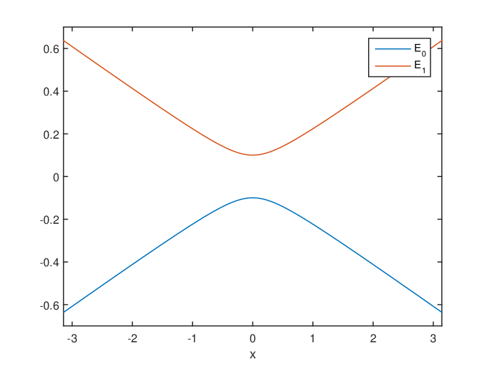
We observe that the two eigenvalue surfaces are close around $x=0$ . By the plots of $d_{01}$ and $D_{01}$ in Figure 1, we see the coupling is significant around $x=0$ as well. To control the energy gap, we introduce the following $F^{\delta}$ function,

F^{\delta}(x)=1+(\delta-1)e^{-10x^{2}},

such that $F^{\delta}(x)=\mathcal{O}(\delta)$ around $x=0$ and $F^{\delta}(0)=\delta$ , so that the energy gap vanishes at $x=0$ as $\delta\to 0$ . The eigenvalues of $H_{e}$ for different values of $\delta$ are plotted in Figure 1.

Refer to caption — Figure 1. (Example 1(a)) Left: Eigenvalues of $H_{e}$ , $\delta=\frac{1}{8}$ , $\frac{1}{16}$ , $\frac{1}{32}$ , $\frac{1}{64}$ and $\frac{1}{128}$ ; reference $\delta=0$ . Right: the coupling information of $H_{e}$ , invariant with respect to $\delta$ .

Example 1(b). Dual avoided crossing. We choose $M$ to be

M=\begin{pmatrix}0&\frac{1}{20}\\ \frac{1}{20}&-e^{-\frac{x^{2}}{10}}+\frac{1}{2}\end{pmatrix},

The eigenvalues of $M$ are

\frac{1}{2}\left(-e^{-\frac{x^{2}}{10}}+\frac{1}{2}\right)\pm\sqrt{\frac{1}{4}\left(-e^{-\frac{x^{2}}{10}}+\frac{1}{2}\right)^{2}+\frac{1}{400}}.

We observe that, the two eigenvalues are closest to each other when $-e^{-\frac{x^{2}}{10}}+\frac{1}{2}=0$ , or $x=\pm\sqrt{10\ln 2}$ . The coupling vectors around these points $x=\pm\sqrt{10\ln 2}$ are significantly larger than their values elsewhere as shown in Figure 2. This explains why the model is often referred to as the dual avoided crossing.

To control the energy gap, we may introduce the following $F^{\delta}$ function,

F^{\delta}(x)=1+e^{-(2\sqrt{10\ln 2})^{2}}+(\delta-1)e^{-(x+\sqrt{10\ln 2})^{2}}+(\delta-1)e^{-(x+\sqrt{2\ln 2})^{2}}.

We can check that $F^{\delta}=\mathcal{O}(\delta)$ around $x=\pm\sqrt{10\ln 2}$ , and

\lim_{\delta\rightarrow 0}F^{\delta}(\pm\sqrt{10\ln 2})=\lim_{\delta\rightarrow 0}\delta\left(1+e^{-(10\sqrt{2\ln 2})^{2}}\right)=0.

Thus the energy gap vanishes at the two points as $\delta\to 0$ . This is illustrated in Figure 2.

Example 1(c). Extended coupling with reflection. In this example, $M$ is set to be

M=\begin{pmatrix}\frac{1}{20}&\frac{1}{10}\left(\arctan(2x)+\frac{\pi}{2}\right)\\ \frac{1}{10}\left(\arctan(2x)+\frac{\pi}{2}\right)&-\frac{1}{20}\end{pmatrix}.

The eigenvalues of $M$ are

\pm\sqrt{\frac{1}{100}\left(\arctan(2x)+\frac{\pi}{2}\right)^{2}+\frac{1}{400}}.

Hence, as $x\rightarrow\infty$ , the eigenvalues of $M$ , $\lambda_{\pm}(x)\rightarrow\pm\frac{\pi}{10}$ , and as $x\rightarrow-\infty$ , the eigenvalues of $M$ , $\lambda_{\pm}(x)\rightarrow\pm\frac{1}{20}$ . As shown in Figure 3, this model involves an extended region of strong non-adiabatic coupling when $x<0$ . Moreover, as $x>0$ , the upper energy surface is increasing so that trajectories moving from left to right on the excited energy surface without a large momentum will be reflected while those on the ground energy surface will be transmitted.

The energy gap between the two surfaces can be controlled by the following $F^{\delta}$ function,

F^{\delta}(x)=\frac{1}{\pi}\left(\arctan(100x)+\frac{\pi}{2}+\delta\right)

We can check that $F^{\delta}=\mathcal{O}(\delta)$ when $x$ is sufficiently small. The family of energy surfaces are illustrated for different values of $\delta$ in Figure 3.

Example 2. Let us mention an example that does not satisfy our assumption in the limit $\delta\to 0$ , which is in fact the classical conical intersection model with

(5.8)

H_{e}^{\delta}(x)=\begin{pmatrix}x&\delta\\ \delta&-x\end{pmatrix}.

In fact, this is the model often analyzed for Landau-Zener transition. For this family of Hamiltonians, we have

\left\lvert E_{+}^{\delta}(x)-E_{-}^{\delta}(x)\right\rvert=2\sqrt{x^{2}+\delta^{2}},

and

\nabla_{x}H_{e}^{\delta}=\begin{pmatrix}1&0\\ 0&-1\end{pmatrix}.

In this case, one can compute the analytical expression for $d_{+-}$ as

d_{+-}^{\delta}(x)=-\frac{\delta}{2(x^{2}+\delta^{2})}.

Clearly, at $x=0$ , $d_{+-}^{\delta}=\mathcal{O}(\delta^{-1})$ . Therefore, around $0$ , Assumption B is violated if $\delta$ goes to zero as $\varepsilon\to 0$ and our theorem no longer applies.

We remark however that for the practical examples with avoided crossing, the small parameters (semiclassical parameter and energy surface gap, etc.) are fixed, rather than converging to $0$ . Therefore, given a particular example, where $H_{e}^{\delta}$ is specified for some small $\delta$ , we can possibly embed the model into a different sequence as $\varepsilon\to 0$ , so that our method can be still used. Some numerical studies are presented in Example 4 for this scenario.

Nevertheless, the fact that the asymptotic derivation breaks down for this particular case raises the question that whether one can combine the fewest switch surface hopping type algorithms with the approaches based on Landau-Zener transition. This will be an interesting future research direction.

6. Numerical examples

In this section, we validate the algorithm based on the frozen Gaussian approximation with surface hopping and its probabilistic interpretation. The numerical examples are done for two-level matrix Schrödinger equations.

6.1. Description of the algorithm

The algorithm based on the stochastic interpretation in Section 3 is straightforward: We sample the initial point of the trajectory based on the weight function $\lvert A^{(0)}(0,z_{0})\rvert$ ; once the initial point is given, we evolve the trajectory and associated FGA variables with surface hopping up to some final time; and then we reconstruct the solution based on the trajectory average (3.15). The value of $A^{(0)}(0,z_{0})$ will be calculated on a mesh of $(q,\,p)$ with numerical quadrature of (2.10).³³ 3 This is of course only possible for low-dimensional examples; approximation methods are needed for higher dimension calculation, which we do not address here. The time evolution ODEs are integrated using the forth-order Runge-Kutta scheme. After each time step, we calculate the hopping probability during the time step $\Delta t|\tau|$ and generate a random number to see if a hop occurs: If a hopping happens, we change the label of the current surface and record the phase factor $\frac{\tau}{|\tau|}$ . After the trajectory is determined up to time $t$ , we can calculate the weighting factors in (3.15) by again a numerical quadrature. Our code is implemented in Matlab.

Note that the algorithm above is the most straightforward Monte Carlo algorithm for evaluating the average of trajectories (3.15). With the path integral representation, it is possible to design more sophisticated algorithms trying to further reduce the variance. This will be considered in future works.

Comparing the numerical solution with the exact solutions to the Schrödinger equations, we have several sources of error, listed below:

a.

Initial error. This is the error coming from numerical quadrature of $A^{(0)}(0,z_{0})$ , the mesh approximation in the phase space, and also due to the choice of a compact domain $K$ in the phase space;
b.

Asymptotic error. This is the $\mathcal{O}(\varepsilon)$ error coming from the higher order term we neglected in the derivation of the frozen Gaussian approximation with surface hopping ansatz;

Sampling error. Since the algorithm is a Monte Carlo algorithm to compute the average of trajectories (3.15), for finite sample size, we will have statistical error compared to the mean value. Since this error is due to the variance of the sampling, it decays as $1/\sqrt{N_{\text{traj}}}$ where $N_{\text{traj}}$ is the total number of trajectories. This is confirmed in Figure 4 and Table 1 for a fixed (and somewhat large) $\varepsilon=\frac{1}{16}$ . In Table 1, convergence rates for tests with different number of trajectories are computed by

\text{Conv. Rate}:=\log_{N^{b}_{\text{traj}}/N^{a}_{\text{traj}}}\frac{\mathbb{E}(e^{a})}{\mathbb{E}(e^{b})}.

$\varepsilon=\frac{1}{16}$	$N_{\text{traj}}=100$	$N_{\text{traj}}=200$	$N_{\text{traj}}=400$	$N_{\text{traj}}=800$	$N_{\text{traj}}=1600$
$\mathbb{E}(e_{0})$	1.9889e-01	1.4182e-01	9.9173e-02	7.2472e-02	5.2443e-02
Conv. Rate		0.4879	0.5160	0.4525	0.4667
$\text{Var}(e_{0})$	2.3702e-03	1.1585e-03	5.6254e-04	3.1891e-04	1.5769e-04
$\mathbb{E}(e_{1})$	1.6423e-01	1.1624e-01	8.1430e-02	6.0873e-02	4.3546e-02
Conv. Rate		0.4987	0.5135	0.4198	0.4833
$\text{Var}(e_{1})$	1.4000e-03	6.5504e-04	3.1067e-04	1.8907e-04	1.0734e-04

Table 1. For

\varepsilon=\frac{1}{16}

and various numbers of trajectories

N_{\text{traj}}

, the empirical averages and sample variance of the total numerical error based on

400

implementations for each test.

d.

Quadrature error. In solving the evolution of FGA variables and make phase changes at hoppings, the ODE solvers will introduce numerical error. Note that, some high order solvers (e.g., RK4 here) are preferred for the FGA variables because in the phase function, the numerical error is magnified by $\mathcal{O}(1/\varepsilon)$ .

In the numerical tests, we use the following initial sampling strategy. We first choose a partition integer $M\in{\mathbb{N}}^{+}$ , and the corresponding partition constant is defined as

d_{M}=\max_{(q,p)\in K}\frac{\bigl\lvert A_{0}^{(0)}\left(0,q,\,p\right)\bigr\rvert}{M}.

For a specific grid point $(q,p)$ , we generate $n_{(q,p)}$ independent trajectories starting with the initial point $(q,p)$ where

n_{(q,p)}=\left\lceil\frac{\bigl\lvert A_{0}^{(0)}\left(0,q,\,p\right)\bigr\rvert}{d_{M}}\right\rceil.

For each trajectory initiated from this grid point, the initial weight $A_{0}^{(0)}(0,q,p)$ is equally divided. As the partition integer $M$ increases, the number of the trajectories increases, and thus the numerical error reduces.

6.2. Numerical tests

All the test problems we consider in this paper are $1D$ two-state matrix Schrödinger equation with the electronic Hamiltonian $H_{e}(x)$ assumed to be a $2\times 2$ matrix potential. We compare with the results from our surface hopping algorithm with the numerical reference solution from the time splitting spectral method (TSSP) (see e.g., [1, 12, 14]) with sufficiently fine mesh.

Example 3. In this example, we take the electronic Hamiltonian $H_{e}(x)$ to be same as Example 1(a) in Section 5.2 with $\delta=\varepsilon$ , which we recall here for convenience,

(6.1)

H_{e}(x)=\left(1+(\varepsilon-1)e^{-10x^{2}}\right)\begin{pmatrix}\frac{\tanh(x)}{2\pi}&\frac{1}{10}\\ \frac{1}{10}&-\frac{\tanh(x)}{2\pi}\end{pmatrix}.

As as shown in Figure 1, the coupling vectors are not negligible when $-1<x<1$ , and hence hopping might occur.

We choose the initial condition to the two-state Schrödinger equation as

u(0,r,x)=u_{0}(0,x)\Psi_{0}(r;x)=(16\varepsilon)^{-1/4}\exp\left(\frac{i2x}{\varepsilon}\right)\exp\left(-16(x-1)^{2}\right)\Psi_{0}(r;x).

this initial condition corresponds to a wave packet in the ground state energy surface localized at $q=-1$ traveling to the right with speed $p=2$ .

Typical FGA trajectories with surface hopping are plotted in Figure 5 for $\varepsilon=\frac{1}{16}$ and $\varepsilon=\frac{1}{128}$ .

For $\varepsilon=\frac{1}{16}$ , $\frac{1}{32}$ and $\frac{1}{64}$ , and for the partition integer $M=1$ , $2$ , $4$ , $8$ , $16$ , we use the FGA algorithm to compute the $u_{0}(t,x)$ and $u_{1}(t,x)$ till $t=1$ . At $t=1$ , the wave packet has traveled across the hopping zone. We choose the computation domain for $y$ and for $x$ to be $[-\pi,\pi]$ , and the computation domain for $(q,p)$ to be $[-\pi,\pi]\times[0.5,3.5]$ . We choose the following mesh sizes in the FGA method for initial sampling and for reconstructing the solution.

(6.2)

\Delta q=\frac{2\pi\varepsilon}{8},\quad\Delta p=\frac{3\varepsilon}{4},\quad\Delta x=\Delta y=\frac{2\pi\varepsilon}{32}.

With this mesh, the initial error $e_{0}^{\varepsilon}$ are summarized in Table 2, which is made significantly smaller than the other parts of the error from the approximation. Also, we choose the step size to be very small $\Delta t=\frac{\epsilon}{32}$ and apply the forth order Runge-Kutta method to solve the FGA variables. Hence, the total error is dominated by the asymptotic error and the sampling error in these tests. The reference solution is computed on $[-\pi,\pi]$ by a second order (in time) TSSP method with sufficiently fine mesh

\Delta x=\frac{2\pi\varepsilon}{64},\quad\Delta t=\frac{\varepsilon}{32}.

$\varepsilon$	$\frac{1}{16}$	$\frac{1}{32}$	$\frac{1}{64}$
$e_{0}^{\varepsilon}$	8.3178e-05	1.4173e-07	1.1697e-07

Table 2. Initial error for

\varepsilon=\frac{1}{16}

\frac{1}{32}

and

\frac{1}{64}

with mesh given by (6.2).

To quantify the sampling error, we repeat each test for $400$ times and estimate the empirical average $\mathbb{E}(e_{k})$ and its variance and $\text{Var}(e_{k})$ are summarized in Table 3, where $e_{k}$ denotes the $L^{2}$ error of the $k$ -th component of the solution, and convergence rates for different $M$ are estimated by

\text{Conv. Rate}:=\log_{M^{b}/M^{a}}\frac{\mathbb{E}(e^{a})}{\mathbb{E}(e^{b})}.

The errors with their $95\%$ confidence intervals are plotted in Figure 6. From the numerical results, we see clearly that increasing the partition integer $M$ can effectively reduce the numerical error.

$\varepsilon=\frac{1}{16}$	$M=1$	$M=2$	$M=4$	$M=8$	$M=16$
$\mathbb{E}(e_{0})$	6.9485e-02	5.5660e-02	4.4370e-02	3.3320e-02	2.6339e-02
Conv. Rate		0.3201	0.3271	0.4132	0.3391
$\text{Var}(e_{0})$	4.9452e-04	2.3494e-04	1.5885e-04	8.7959e-05	5.5006e-05
$\mathbb{E}(e_{1})$	5.7770e-02	4.6380e-02	3.8663e-02	3.0728e-02	2.5886e-02
Conv. Rate		0.3168	0.2626	0.3314	0.2474
$\text{Var}(e_{1})$	2.7984e-04	1.3865e-04	1.0308e-04	6.0901e-05	4.8058e-05

$\varepsilon=\frac{1}{32}$	$M=1$	$M=2$	$M=4$	$M=8$	$M=16$
$\mathbb{E}(e_{0})$	5.6999e-02	4.6254e-02	3.5705e-02	2.6951e-02	2.0107e-02
Conv. Rate		0.3014	0.3735	0.4058	0.4227
$\text{Var}(e_{0})$	2.8623e-04	1.5798e-04	1.0331e-04	5.2099e-05	2.8266e-05
$\mathbb{E}(e_{1})$	5.2574e-02	4.2267e-02	3.3255e-02	2.5514e-02	2.0454e-02
Conv. Rate		0.3149	0.3460	0.3823	0.3189
$\text{Var}(e_{1})$	1.8928e-04	1.2575e-04	6.7133e-05	4.0982e-05	2.6102e-05

$\varepsilon=\frac{1}{64}$	$M=1$	$M=2$	$M=4$	$M=8$	$M=16$
$\mathbb{E}(e_{0})$	4.8308e-02	3.8534e-02	2.9118e-02	2.2112e-02	1.6811e-02
Conv. Rate		0.3261	0.4042	0.3970	0.3955
$\text{Var}(e_{0})$	1.9927e-04	9.3424e-05	5.0794e-05	3.1704e-05	1.7614e-05
$\mathbb{E}(e_{1})$	4.6589e-02	3.6833e-02	2.8203e-02	2.1660e-02	1.6785e-02
Conv. Rate		0.3390	0.3852	0.3808	0.3678
$\text{Var}(e_{1})$	1.5864e-04	8.1220e-05	5.4446e-05	2.6814e-05	1.5051e-05

Table 3. (Example 3) For various

\varepsilon

and partition integers

M

, the empirical averages and sample variance of the total numerical error based on

400

implementations for each test.

Finally, we aim to demonstrate the application of the FGA-SH method in calculating the transition rate versus time. For $\varepsilon=\frac{1}{16}$ and $\frac{1}{128}$ , we carry out the test with $N_{\text{traj}}=6400$ trajectories, and calculate the transition rates at different times till $t=1.5$ . The results are plotted in Figure 7, from which we observe very nice agreements with the reference calculations.

Example 4. In this example, the electronic Hamiltonian $H_{e}(x)$ is given by

(6.3)

H_{e}(x)=\begin{pmatrix}\frac{x}{5}&\frac{1}{10}\\ \frac{1}{10}&-\frac{x}{5}\end{pmatrix}.

This matrix potential is similar to the Example 2 in Section 5.2 except that the we have fixed a small $\delta$ as $\varepsilon$ varies. Hence, as $\varepsilon$ goes to $0$ , the energy surfaces of the electronic Hamiltonian stay unchanged. Thus, the FGA method applies to this case. We plot the energy surfaces, $d_{01}$ and $D_{01}$ of this matrix potential in Figure 8, from which we observe that the coupling vector is not negligible around $x=0$ .

We choose the same initial condition to the two-state Schrödinger equation

u(0,r,x)=u_{0}(0,x)\Psi_{0}(r;x)=\exp\left(\frac{i2x}{\varepsilon}\right)\exp\left(-16(x-1)^{2}\right)\Psi_{0}(r;x),

and the same computation domain and meshing sizes for the FGA algorithm and reference solver as Example 3. For $\varepsilon=\frac{1}{16}$ and $\frac{1}{128}$ , and for the partition integer $16$ , we use the FGA algorithm to compute the $u_{0}(t,x)$ and $u_{1}(t,x)$ till $t=1$ .

The reference solution indicates that when $\varepsilon=\frac{1}{16}$ , the transition portion is significant but when $\varepsilon=\frac{1}{128}$ the transition between the surfaces is practically small. This is expected as the gap is finite and fixed, while $\varepsilon\rightarrow 0$ , so that the non-adiabatic transition is approaching $0$ (see e.g., [25, 23]).

Whereas, in the FGA algorithm, the hopping rate is only related to the coupling vectors and the momentum along the FGA trajectory. Therefore, for $\varepsilon=\frac{1}{16}$ and $\frac{1}{128}$ , the hopping probabilities are similar along the FGA trajectory, but when $\varepsilon=\frac{1}{128}$ , the hopped trajectories on the exited state should average to $0$ , which is verified by the numerical results plotted in Figure 9 together with the reference solution. Besides, we show by comparing the reference solutions in Figure 9 that the weighting factors in (3.15) are crucial in reconstructing the correct wave functions.

7. Convergence proof

We now prove that the ansatz is a good approximation to the true solution of the matrix Schrödinger equation. For simplicity of notations, we omit the appearance of $\delta$ in the surface energy and coupling vectors. By Assumption B, the boundedness of related quantities in the following analysis is uniform with respect to $\delta$ , and hence all the estimates below are independent of $\delta$ . In §7.1, we study the trajectories, which follow Hamiltonian flows on each energy surfaces with hopping between surfaces. The absolute convergence of the infinite sum used in the surface hopping ansatz is shown in §7.2. Finally, in §7.3, we prove the main convergence result Theorem 5.1.

7.1. Preliminaries

To study the absolute convergence of the FGA with surface hopping ansatz, we fix a time $t$ and recall that

(7.1)

U_{\text{FGA}}(t,x)=\sum_{k=0}^{\infty}\begin{pmatrix}u^{(2k)}\\ u^{(2k+1)}\end{pmatrix}.

For convenience of the readers, we also recall

(7.2)

u^{(j)}(t,x)=\frac{1}{(2\pi\varepsilon)^{3m/2}}\int_{K}\,\mathrm{d}z_{0}\int_{0<t_{1}<\cdots<t_{j}<t}dT_{j:1}\;\tau^{(1)}(T_{1:1},z_{0})\cdots\tau^{(j)}(T_{j:1},z_{0})\times\\ \times A^{(j)}(t,T_{j:1},z_{0})\exp\left(\frac{i}{\varepsilon}\Theta^{(j)}(t,T_{j:1},z_{0},x)\right),

which is an integration over all possible $j$ hopping times $t_{1},\cdots,t_{j}$ . Notice that as discussed above Theorem 5.1, we restrict the domain of integration on the phase space to $K$ .

Also recall that the FGA variables in the integrand of each $u^{(j)}$ are evolved piecewisely to final time $t$ . To be more specific, the hopping time sequence $\{t_{k}\}_{k=1,\cdots,j}$ defines a partition of the interval $[0,t]$ , $0\leqslant t_{1}\leqslant\cdots\leqslant t_{j}\leqslant t$ , such that within each interval, the FGA trajectory and associated variables evolve on a single energy surface, and at hopping times $\{t_{k}\}_{k=1,\cdots,j}$ switch to another surface with the continuity conditions (2.14).

We remark that since we study here the case with two energy surfaces, it suffices to specify the hopping times to uniquely determine the trajectory. In general, for more energy surfaces, besides the hopping time, we also need to track which surface the trajectory hops to (which makes the notations more complicated).

Let us first collect some properties of the Hamiltonian flow with surface hopping. Given the hopping times $T_{j:1}=\{t_{j},\cdots,t_{1}\}$ , we denote the map on the phase space from initial time $0$ to time $t$ by $\kappa_{t,T_{j:1}}$ ( $t$ can be smaller than $t_{j}$ here):

	$\displaystyle\kappa_{t,T_{j:1}}:\quad{\mathbb{R}}^{2m}$	$\displaystyle\rightarrow{\mathbb{R}}^{2m}$
	$\displaystyle(q,p)$	$\displaystyle\longmapsto\left(Q^{\kappa_{t,T_{j:1}}}(q,p),P^{\kappa_{t,T_{j:1}}}(q,p)\right),$

such that

(7.3)

\bigl(Q^{\kappa_{t,T_{j:1}}}(q,p),P^{\kappa_{t,T_{j:1}}}(q,p)\bigr)=\begin{cases}\bigl(Q^{(0)}(t,q,p),P^{(0)}(t,q,p)\bigr),&t\leqslant T_{1};\\ \bigl(Q^{(i)}(t,T_{i:1},q,p),P^{(i)}(t,T_{i:1},q,p)\bigr),&t\in[T_{i},T_{i+1}],i\in\{1,\ldots,j\};\\ \bigl(Q^{(j)}(t,T_{j:1},q,p),P^{(j)}(t,T_{j:1},q,p)\bigr),&t\geqslant T_{j},\end{cases}

where the trajectory follows the Hamiltonian flow on one of the energy surface and hops to the other at the hopping times. Let us emphasize that, due to the continuity condition (2.14), even with surface hopping, the trajectory $(Q,P)$ is still continuous on the phase space as a function of $t$ .

The following proposition states that for any possible number of hops and sequence of hopping time, the trajectory under $\kappa_{t,T}$ remains (uniformly) in a compact set.

Proposition 7.1.

Given $t>0$ and a compact subset $K\subset{\mathbb{R}}^{2m}$ , there exists a compact set $K_{t}\subset{\mathbb{R}}^{2m}$ , such that $\forall j\in{\mathbb{N}}$ , $\forall\delta>0$ and any sequence of hopping times $T_{j:1}\subset[0,t]$

(7.4)

\kappa_{t,T_{j:1}}(K)\subset K_{t},

namely, for any $(q,p)\in K$ and any $s\in[0,t]$

(7.5)

\left(Q^{\kappa_{s,T_{j:1}}}(q,p),P^{\kappa_{s,T_{j:1}}}(q,p)\right)\in K_{t}.

Proof.

Fix an arbitrary sequence of hopping time $T_{j:1}\subset[0,t]$ . For any time $s\in[0,t]$ which belongs to one of the interval $(t_{k},t_{k+1})$ for $k=0,\cdots,j$ (we identify $t_{0}=0$ and $t_{j+1}=t$ ). Denote the index of the energy surface during the time interval $(t_{k},t_{k+1})$ as $l_{k}$ , we then have

		$\displaystyle\frac{\,\mathrm{d}}{\,\mathrm{d}s}\left\lvert P^{\kappa_{s,T_{j:1}}}\right\rvert=\frac{P^{\kappa_{s,T_{j:1}}}}{\left\lvert P^{\kappa_{s,T_{j:1}}}\right\rvert}\cdot\frac{\,\mathrm{d}}{\,\mathrm{d}s}P^{\kappa_{s,T_{j:1}}}=-\frac{P^{\kappa_{s,T_{j:1}}}\cdot\nabla_{Q}E_{l_{k}}}{\left\lvert P^{\kappa_{s,T_{j:1}}}\right\rvert}\leqslant C_{E}\Bigl(\left\lvert Q^{\kappa_{s,T_{j:1}}}\right\rvert+1\Bigr),$
		$\displaystyle\frac{\,\mathrm{d}}{\,\mathrm{d}s}\left\lvert Q^{\kappa_{s,T_{j:1}}}\right\rvert=\frac{Q^{\kappa_{s,T_{j:1}}}}{\left\lvert Q^{\kappa_{s,T_{j:1}}}\right\rvert}\cdot\frac{\,\mathrm{d}}{\,\mathrm{d}s}Q^{\kappa_{s,T_{j:1}}}=\frac{Q^{\kappa_{s,T_{j:1}}}\cdot P^{\kappa_{s,T_{j:1}}}}{\left\lvert Q^{\kappa_{s,T_{j:1}}}\right\rvert}\leqslant\left\lvert P^{\kappa_{s,T_{j:1}}}\right\rvert,$

where we have used the subquadraticity of the Hamiltonian by Assumption A (recall that $C_{E}$ is uniform with respect to $\delta$ ). Therefore,

\frac{\,\mathrm{d}}{\,\mathrm{d}s}\Bigl(\left\lvert P^{\kappa_{s,T_{j:1}}}\right\rvert^{2}+\left\lvert Q^{\kappa_{s,T_{j:1}}}\right\rvert^{2}\Bigr)\leqslant 2(C_{E}+1)\left\lvert P^{\kappa_{s,T_{j:1}}}\right\rvert\Bigl(\left\lvert Q^{\kappa_{s,T_{j:1}}}\right\rvert+1\Bigr)\leqslant 2(C_{E}+1)\Bigl(\left\lvert P^{\kappa_{s,T_{j:1}}}\right\rvert^{2}+\left\lvert Q^{\kappa_{s,T_{j:1}}}\right\rvert^{2}+1\Bigr).

Here we emphasize that the constant on the right hand side is universal in the sense that it does not depend on the particular hopping time sequence. The conclusion of the Proposition follows immediately from the differential inequality. ∎

As a corollary, since the trajectory uniformly stays in a compact set, given the final time $t$ , we can take a constant $C_{\tau}$ such that the following estimate holds

(7.6)

\sup_{z_{0}\in K,T_{n:1}\subset[0,t],n\in{\mathbb{N}}^{+},\,i=0,1}|\tau_{i}^{(n)}(T_{n:1},z_{0})|\leqslant\sup_{z\in K_{t}}\max\bigl\{\lvert p\cdot d^{\delta}_{10}(q)\rvert,\lvert p\cdot d^{\delta}_{01}(q)\rvert\bigr\}\leq C_{\tau},

where the second inequality uses Assumption B and recall that the constants are uniform with respect to $\delta$ . Thus, the coupling coefficient stays $\mathcal{O}(1)$ along all possible FGA trajectories.

For a transformation of the phase space $\kappa:{\mathbb{R}}^{2m}\to{\mathbb{R}}^{2m}$ , we denote its Jacobian matrix as

(7.7)

J^{\kappa}(q,p)=\begin{pmatrix}\left(\partial_{q}Q^{\kappa}\right)^{T}(q,p)&\left(\partial_{p}Q^{\kappa}\right)^{T}(q,p)\\ \left(\partial_{q}P^{\kappa}\right)^{T}(q,p)&\left(\partial_{p}P^{\kappa}\right)^{T}(q,p)\end{pmatrix}.

We say the transform $\kappa$ is a canonical if $J^{\kappa}$ is symplectic for any $(q,p)\in{\mathbb{R}}^{2m}$ , namely,

(7.8)

\left(J^{\kappa}\right)^{T}\begin{pmatrix}0&I_{m}\\ -I_{m}&0\end{pmatrix}J^{\kappa}=\begin{pmatrix}0&I_{m}\\ -I_{m}&0\end{pmatrix}.

Here, $I_{m}$ denotes the $m\times m$ identity matrix.

The map given by the FGA trajectories $\kappa_{t}$ is always canonical, as stated in the following proposition, which also gives bounds of the Jacobian and its derivatives.

Proposition 7.2.

Given $t>0$ and a compact subset $K\subset{\mathbb{R}}^{2m}$ , the associated map $\kappa_{t,T_{j:1}}$ is a canonical transformation for any sequence of hopping times $T_{j:1}$ , $\forall\,j$ . Moreover, for any $k\in{\mathbb{N}}$ , there exists a constant $C_{k}$ such that

(7.9)

\sup_{(q,p)\in K}\max_{\lvert\alpha_{p}\rvert+\lvert\alpha_{q}\rvert\leqslant k}\left\lvert\partial_{q}^{\alpha_{q}}\partial_{p}^{\alpha_{p}}\bigl[J^{\kappa_{t,T_{j:1}}}(q,p)\bigr]\right\rvert\leqslant C_{k},

uniformly for any $j\in{\mathbb{N}}$ , any $\delta$ and any sequence of hopping times $T_{j:1}$ .

Proof.

Recall that the time evolution of $(Q^{\kappa},P^{\kappa})$ is piecewisely defined in the time interval between hoppings, and remains continuous at the hopping times. During each time interval, the symplectic condition (7.8) is clearly satisfied by the Hamiltonian flow. The continuity condition guarantees the validity of symplectic relation at the hopping times. Therefore, the map $\kappa_{t,T_{j:1}}$ is a canonical transform.

For any time $s\in[0,t]$ which belongs to one of the interval $(t_{k},t_{k+1})$ for $k=0,\cdots,j$ (we identify $t_{0}=0$ and $t_{j+1}=t$ ). Denote the index of the energy surface during the time interval $(t_{k},t_{k+1})$ as $l_{k}$ , we then have by differentiating $J^{\kappa_{s,T_{j:1}}}$ with respect to $s$

(7.10)

\frac{\,\mathrm{d}}{\,\mathrm{d}s}J^{\kappa_{s,T_{j:1}}}=\begin{pmatrix}\partial_{P}\partial_{Q}H_{l_{k}}&\partial_{P}\partial_{P}H_{l_{k}}\\ -\partial_{Q}\partial_{Q}H_{l_{k}}&-\partial_{Q}\partial_{P}H_{l_{k}}\end{pmatrix}J^{\kappa_{s,T_{j:1}}}.

Then, Assumption A implies there exists a constant $C$ such that

(7.11)

\frac{\,\mathrm{d}}{\,\mathrm{d}s}\left\lvert J^{\kappa_{s,T_{j:1}}}\right\rvert\leqslant\left\lvert\begin{pmatrix}\partial_{P}\partial_{Q}H_{l_{k}}&\partial_{P}\partial_{P}H_{l_{k}}\\ -\partial_{Q}\partial_{Q}H_{l_{k}}&-\partial_{Q}\partial_{P}H_{l_{k}}\end{pmatrix}\right\rvert\left\lvert J^{\kappa_{s,T_{j:1}}}\right\rvert\leqslant C\left\lvert J^{\kappa_{s,T_{j:1}}}\right\rvert.

It is worth emphasizing that this constant $C$ is independent of the hopping time sequence and $\delta$ . The boundedness of $|J^{\kappa_{t,T_{j:1}}}|$ then follows immediately from Gronwall’s inequality and the fact that $|J^{\kappa_{0,T_{j:1}}}|=1$ since $\kappa_{0,T_{j:1}}$ is just an identity map. To get the estimate for derivatives of $J$ , we differentiate the equation (7.10) with respect to $(q,p)$ and use an induction argument, and we omit the straightforward calculations here. ∎

For a canonical transform $\kappa$ , we define

Z^{\kappa}(q,p)=\partial_{z}\left(Q^{\kappa}(q,p)+iP^{\kappa}(q,p)\right),

where $\partial_{z}=\partial_{q}-i\partial_{p}$ . $Z^{\kappa}$ is a complex valued $m\times m$ matrix. By mimicking the proof of [22]*Lemma 5.1 and the above Proposition, we obtain the following properties of $Z^{\kappa}$ .

Proposition 7.3.

Given $t>0$ and a compact subset $K\subset{\mathbb{R}}^{2m}$ , for any sequence of hopping times $T_{j:1}$ , $\forall\,j$ , $Z^{\kappa_{t,T_{j:1}}}$ is invertible. Moreover, for any $k\in{\mathbb{N}}$ , there exists a constant $C_{k}$ such that

(7.12)

\sup_{(q,p)\in K}\max_{\lvert\alpha_{p}\rvert+\lvert\alpha_{q}\rvert\leqslant k}\left\lvert\partial_{q}^{\alpha_{q}}\partial_{p}^{\alpha_{p}}\bigl[\bigl(Z^{\kappa_{t,T_{j:1}}}(q,p)\bigr)^{-1}\bigr]\right\rvert\leqslant C_{k},

uniformly for any $j\in{\mathbb{N}}$ , any $\delta>0$ and any sequence of hopping times $T_{j:1}$ .

For the frozen Gaussian approximation, it is useful to introduce the following Fourier integral operator. For $M\in L^{\infty}({\mathbb{R}}^{2m};{\mathbb{C}})$ , $u\in\mathcal{S}({\mathbb{R}}^{m};{\mathbb{C}})$ , and a FGA flow denoted by $\kappa_{t,T_{j:1}}$ with $T_{j:1}\subset[0,t]$ , we define

(7.13)

\Bigl(\mathcal{I}_{\kappa_{t,T_{j:1}}}^{\varepsilon}(M)u\Bigr)(x)=(2\pi\varepsilon)^{-\frac{3m}{2}}\int_{{\mathbb{R}}^{m}}\int_{{\mathbb{R}}^{2m}}\exp\Bigl(\frac{i}{\varepsilon}\Phi^{(j)}(t,x,y,z)\Bigr)M(z)u(y)\,\mathrm{d}z\,\mathrm{d}y,

where the phase function $\Phi^{(j)}$ is given by

\Phi^{(j)}(t,x,y,z)=S^{(j)}(t,T_{j:1},z)+\frac{i}{2}\bigl\lvert x-Q^{(j)}(t,T_{j:1},z)\bigr\rvert^{2}+P^{(j)}(t,T_{j:1},z)\cdot\bigl(x-Q^{(j)}(t,T_{j:1},z)\bigr)+\frac{i}{2}|y-q|^{2}-p\cdot(y-q),

where the FGA variables $P^{(j)},Q^{(j)},S^{(j)}$ are evolved as in the surface hopping ansatz, with given $t$ and the hopping time sequence $T_{j:1}$ . With this Fourier integral operator, we may rewrite the surface hopping ansatz (2.11) for $u_{0}^{(n)}$ as

u_{0}^{(n)}(t)=\int_{0<t_{1}<\cdots<t_{n}<T}\,\mathrm{d}T_{n:1}\;\mathcal{I}_{\kappa_{t,T_{n:1}}}^{\varepsilon}\Bigl(a_{i}^{(n)}\prod_{j=1}^{n}\tau_{i}^{(j)}\chi_{K}\Bigr)u_{0}(0),

where $\chi_{K}$ is the characteristic function on the set $K$ , which restricts the initial $z_{0}$ in the FGA ansatz. This representation is particularly convenient for our estimates, as we have the following proposition for the norm of the Fourier integral operators. The version of Proposition without hopping was proved in [22]*Proposition 3.7. The proof in fact can be almost verbatim used in the current situation (with some notational change), and thus we skip the details here.

Proposition 7.4.

For any $t$ and any hopping time sequence $\{t_{1},t_{2},\cdots,t_{j}\}$ for $\forall\,j\in{\mathbb{N}}$ , denoting the the symplectic transform for the FGA with surface hopping flow as $\kappa_{t,T_{j:1}}$ , the operator $\mathcal{I}_{\kappa_{t,T_{j:1}}}^{\varepsilon}(M)$ can be extended to a linear bounded operator on $L^{2}({\mathbb{R}}^{m},{\mathbb{C}})$ , and we have

(7.14)

\biggl\lVert\mathcal{I}_{\kappa_{t,T_{j:1}}}^{\varepsilon}(M)\biggr\rVert_{\mathcal{L}(L^{2}({\mathbb{R}}^{m};\,{\mathbb{C}}))}\leqslant 2^{-\frac{m}{2}}\lVert M\rVert_{L^{\infty}({\mathbb{R}}^{2m};\,{\mathbb{C}})}.

7.2. Absolute convergence of surface hopping ansatz

Now we estimate the contribution of the terms in the FGA ansatz.

Proposition 7.5.

For a given time $t$ , there exists a constant $C_{a}$ , depending only on $t$ and the initial conditions of the FGA variables, such that for any $n\in{\mathbb{N}}$ and any hopping moment sequence $T_{n:1}\subset[0,t]$ , it holds

(7.15)

\Biggl\lVert\frac{1}{(2\pi\varepsilon)^{3m/2}}\int_{K}\,\mathrm{d}z_{0}\;\prod_{j=1}^{n}\tau^{(j)}(T_{j:1},z_{0})A^{(n)}(t,T_{n:1},z_{0})\exp\Bigl(\frac{i}{\varepsilon}\Theta^{(n)}\bigl(t,T_{n:1},z_{0},x\bigr)\Bigr)\Biggr\rVert_{L^{2}({\mathbb{R}}^{m})}\leqslant C_{a}.

Proof.

Recall that we have

\frac{1}{(2\pi\varepsilon)^{3m/2}}\int_{K}\,\mathrm{d}z_{0}\;\prod_{j=1}^{n}\tau^{(j)}(T_{j:1},z_{0})A^{(n)}(t,T_{n:1},z_{0})\exp\Bigl(\frac{i}{\varepsilon}\Theta^{(n)}(T,T_{n:1},z_{0},x)\Bigr)\\ =\Bigl(\mathcal{I}_{\kappa_{t,T_{n:1}}}^{\varepsilon}\Bigl(\prod_{j=1}^{n}\tau^{(j)}(T_{j:1},\cdot)a^{(n)}(t,T_{n:1},\cdot)\chi_{K}\Bigr)u_{0}(0)\Bigr)(x).

Thus, using Proposition 7.4 and the bound (7.6) for the hopping coefficient $\tau$ ’s, it suffices to control $a^{(n)}(t,T_{n:1},z_{0})$ for $z_{0}\in K$ . Recall that

A^{(k)}(t,T_{k:1},z_{0})=a^{(k)}(t,T_{k:1},z_{0})\int_{{\mathbb{R}}^{m}}u_{0}(0,y)e^{\frac{i}{\varepsilon}(-p\cdot(y-q)+\frac{i}{2}|y-q|^{2})}\,\mathrm{d}y,

and hence $a^{(k)}$ satisfies the same linear equation as those for $C^{(k)}$ with the continuity conditions at the hopping times: Depending on whether $k$ is even or odd

	$\displaystyle\frac{\,\mathrm{d}}{\,\mathrm{d}t}a^{(k)}$	$\displaystyle=\frac{1}{2}a^{(k)}\tr\left((Z^{(k)})^{-1}\left(\partial_{z}P^{(k)}-i\partial_{z}Q^{(k)}\nabla^{2}_{Q}E_{0}(Q^{(k)})\right)\right)-a^{(k)}d_{00}\cdot P^{(k)},\qquad k\text{ even};$
	$\displaystyle\frac{\,\mathrm{d}}{\,\mathrm{d}t}a^{(k)}$	$\displaystyle=\frac{1}{2}a^{(k)}\tr\left((Z^{(k)})^{-1}\left(\partial_{z}P^{(k)}-i\partial_{z}Q^{(k)}\nabla^{2}_{Q}E_{1}(Q^{(k)})\right)\right)-a^{(k)}d_{11}\cdot P^{(k)},\qquad k\text{ odd}.$

Note that the coefficients on the right hand side are all uniformly bounded along the trajectory thanks to (7.5), (7.6), (7.9), and (7.12) in the preliminaries. Therefore, $a^{(n)}$ is also bounded uniformly with respect to all hopping sequences, which concludes the proof. ∎

With Proposition 7.5, we further estimate the contribution $u^{(n)}$ in the surface hopping ansatz.

Theorem 7.6.

Under Assumptions A and B, given a fixed final time $t$ , there exist constants $C_{t}$ and $C$ , independent of $\varepsilon$ and $\delta$ , such that for any $n\in{\mathbb{N}}$ , we have

\left\lVert u^{(n)}(t,x)\right\rVert_{L^{2}({\mathbb{R}}^{m})}\leqslant C\frac{(C_{t})^{n}}{n!},\quad\text{and}\quad\left\lVert\varepsilon\nabla_{x}u^{(n)}(t,x)\right\rVert_{L^{2}({\mathbb{R}}^{m})}\leqslant C\frac{(C_{t})^{n}}{n!}.

In particular, the surface hopping ansatz (4.16) is absolutely convergent.

Proof.

Note that

u^{(n)}=\int_{0<t_{1}<\cdots<t_{n}<t}\,\mathrm{d}T_{n:1}\;\mathcal{I}_{\kappa_{t,T_{n:1}}}^{\varepsilon}\Bigl(\prod_{j=1}^{n}\tau^{(j)}(T_{j:1},\cdot)a^{(n)}(t,T_{n:1},\cdot)\chi_{K}\Bigr)u_{0}.

We estimate using Proposition 7.5

	$\displaystyle\left\lVert u^{(n)}\right\rVert_{L^{2}({\mathbb{R}}^{m})}$	$\displaystyle\leqslant\int_{0<t_{1}<\cdots<t_{n}<t}\,\mathrm{d}T_{n:1}\;\Biggl\lVert\mathcal{I}_{\kappa_{t,T_{n:1}}}^{\varepsilon}\Bigl(\prod_{j=1}^{n}\tau^{(j)}(T_{j:1},\cdot)a^{(n)}(t,T_{n:1},\cdot)\chi_{K}\Bigr)u_{0}\Biggr\rVert_{L^{2}({\mathbb{R}}^{m})}$
		$\displaystyle\leqslant C\int_{0<t_{1}<\cdots<t_{n}<t}\,\mathrm{d}T_{n:1}\;C_{\tau}^{n}=C\frac{(tC_{\tau})^{n}}{n!}$

The absolute convergence of $U_{\text{FGA}}(t,x)$ then follows from dominated convergence.

The control of $\varepsilon\nabla_{x}u^{(n)}$ is quite similar, except that we shall use Lemma 2.2 to control the term $(x-Q^{(n)})$ resulting from the gradient. Actually,

(7.16)

\varepsilon\nabla_{x}u^{(n)}(t,x)=\frac{1}{(2\pi\varepsilon)^{3m/2}}\int_{K}\,\mathrm{d}z_{0}\int_{0<t_{1}<\cdots<t_{n}<t}\,\mathrm{d}T_{n:1}\;\tau^{(1)}(T_{1:1},z_{0})\cdots\tau^{(n)}(T_{n:1},z_{0})\times\\ \times i\left(P^{(n)}+i(x-Q^{(n)})\right)A^{(n)}(t,T_{n:1},z_{0})\exp\left(\frac{i}{\varepsilon}\Theta^{(n)}(t,T_{n:1},z_{0},x)\right).

The control of the term involving $P^{(n)}$ is the same as that of $u^{(n)}$ . By Lemma 2.2, the term involving $(x-Q^{(n)})$ is an even smaller term, which follows from the estimate (7.12) and a slight variation of Proposition 7.5. ∎

7.3. The analysis of approximation error

We now estimate the approximation error of the FGA approximation with surface hopping to the matrix Schrödinger equation (2.3). We first state a consistency result by estimating the error of substituting $U_{\text{FGA}}$ into (2.3). All the estimates and constants below are uniform in $\delta$ .

Theorem 7.7.

Under Assumptions A and B, given a final time $t$ , there exists a constant $C_{t}$ , such that

\Biggl\lVert i\varepsilon\partial_{t}U_{\text{FGA}}+\frac{\varepsilon^{2}}{2}\Delta_{x}U_{\text{FGA}}+\begin{pmatrix}E_{0}\\ &E_{1}\end{pmatrix}U_{\text{FGA}}-\frac{\varepsilon^{2}}{2}\begin{pmatrix}D_{00}&D_{01}\\ D_{10}&D_{11}\end{pmatrix}U_{\text{FGA}}-\varepsilon^{2}\sum_{j=1}^{m}\begin{pmatrix}d_{00}&d_{01}\\ d_{10}&d_{11}\end{pmatrix}_{j}\partial_{x_{j}}U_{\text{FGA}}\Biggl\rVert_{L^{2}({\mathbb{R}}^{m})}\leqslant\varepsilon^{2}e^{C_{t}}.

Proof.

We first consider the term arises from the time derivative and denote for $j$ even

I^{j}_{1}+I^{j}_{2}=i\varepsilon\partial_{t}\begin{pmatrix}u_{0}^{(j)}\\ 0\end{pmatrix},

where

(7.17)

I^{j}_{1}=\begin{pmatrix}\displaystyle i\varepsilon\frac{1}{(2\pi\varepsilon)^{3m/2}}\int_{K}\,\mathrm{d}z_{0}\int_{0<t_{1}<\cdots<t_{j}<t}\,\mathrm{d}T_{j:1}\;\tau^{(1)}\cdots\tau^{(j)}\partial_{t}\Bigl[A^{(j)}\exp\Bigl(\frac{i}{\varepsilon}\Theta^{(j)}\Bigr)\Bigr]\\ 0\end{pmatrix}

coming from the time derivative acting on the integrand, and for $j\geqslant 1$ ,

(7.18)

I^{j}_{2}=\begin{pmatrix}\displaystyle i\varepsilon\frac{1}{(2\pi\varepsilon)^{3m/2}}\left[\int_{K}\,\mathrm{d}z_{0}\int_{0<t_{1}<\cdots<t_{j}<t}\,\mathrm{d}T_{j:1}\;\tau^{(1)}\cdots\tau^{(j)}A^{(j)}\exp\Bigl(\frac{i}{\varepsilon}\Theta_{0}^{(j)}\Bigr)\right]_{t_{j}=t}\\ 0\end{pmatrix}

resulting from the time derivative acting on the upper limit of the integral. The expression for odd $j$ is similar except that the top and bottom rows are flipped: $i\varepsilon\partial_{t}\bigl(\begin{smallmatrix}0\\ u_{0}^{(j)}\end{smallmatrix}\bigr)$ .

We also write the terms from the right hand side of (2.3) for even $j$ as:

I^{j}_{3}+I^{j}_{4}=-\frac{\varepsilon^{2}}{2}\Delta_{x}\begin{pmatrix}u^{(j)}\\ 0\end{pmatrix}+\begin{pmatrix}E_{0}\\ &E_{1}\end{pmatrix}\begin{pmatrix}u^{(j)}\\ 0\end{pmatrix}-\frac{\varepsilon^{2}}{2}\begin{pmatrix}D_{00}&D_{01}\\ D_{10}&D_{11}\end{pmatrix}\begin{pmatrix}u^{(j)}\\ 0\end{pmatrix}-\varepsilon^{2}\sum_{j=1}^{d}\begin{pmatrix}d_{00}&d_{01}\\ d_{10}&d_{11}\end{pmatrix}_{j}\partial_{x_{j}}\begin{pmatrix}u^{(j)}\\ 0\end{pmatrix}

where

(7.19)		$\displaystyle I^{j}_{3}$	$\displaystyle=\begin{pmatrix}\bigl(H_{0}-\frac{\varepsilon^{2}}{2}D_{00}\bigr)u^{(j)}-\varepsilon^{2}d_{00}\cdot\nabla_{x}u^{(j)}\\ 0\end{pmatrix},$
(7.20)		$\displaystyle I^{j}_{4}$	$\displaystyle=\begin{pmatrix}0\\ -\varepsilon^{2}d_{01}\cdot\nabla_{x}u^{(j)}-\frac{\varepsilon^{2}}{2}D_{01}u^{(j)}\end{pmatrix}.$

Here, $I^{j}_{3}$ contains all the terms which govern the inner-surface evolution on each energy surface, while $I^{j}_{4}$ contains the coupling terms (note that the subscripts are swapped). The expressions for odd $j$ is similar.

Denote $U_{\text{FGA}}^{n}$ the sum of the first $n$ terms in the FGA ansatz (7.1). Summing over the contributions up to $u^{(n)}$ , we have

i\varepsilon\partial_{t}U_{\text{FGA}}^{n}+\frac{\varepsilon^{2}}{2}\Delta_{x}U_{\text{FGA}}^{n}+\begin{pmatrix}E_{0}\\ &E_{1}\end{pmatrix}U_{\text{FGA}}^{n}-\frac{\varepsilon^{2}}{2}\begin{pmatrix}D_{00}&D_{01}\\ D_{10}&D_{11}\end{pmatrix}U_{\text{FGA}}^{n}-\varepsilon^{2}\sum_{j=1}^{d}\begin{pmatrix}d_{00}&d_{01}\\ d_{10}&d_{11}\end{pmatrix}_{j}\partial_{x_{j}}U_{\text{FGA}}^{n}\\ =\sum_{j=0}^{n}I^{j}_{1}+\sum_{j=1}^{n}I^{j}_{2}-\sum_{j=0}^{n}I^{j}_{3}-\sum_{j=0}^{n}I^{j}_{4}=\sum_{j=0}^{n}\left(I^{j}_{1}-I^{j}_{3}\right)+\sum_{j=0}^{n-1}\left(I^{j+1}_{2}-I^{j}_{4}\right)+I^{n}_{4}.

We now estimate three terms on the right hand side.

Term $I_{4}^{n}$ : By Theorem 7.6, we have

(7.21)

\displaystyle\bigl\lVert I_{4}^{n}\bigr\rVert_{L^{2}({\mathbb{R}}^{m})}

\displaystyle\leqslant C\varepsilon\lVert\varepsilon\nabla_{x}u^{(j)}\rVert_{L^{2}({\mathbb{R}}^{m})}+C\varepsilon^{2}\lVert u^{(j)}\rVert_{L^{2}({\mathbb{R}}^{m})}\leqslant C\varepsilon\frac{(C_{t})^{n}}{n!}.

Term $\sum(I^{j}_{1}-I^{j}_{3})$ : The difference $(I^{j}_{1}-I^{j}_{3})$ contains all the formally $O(\varepsilon^{2})$ terms we have dropped in determining the equation for $A^{(j)}$ . To estimate those, we use the Taylor expansions with respect the beam center $Q$

	$\displaystyle E_{k}(x)$	$\displaystyle=\sum_{\|\alpha\|\leqslant 3}\frac{\partial_{\alpha}E_{k}(Q)}{\alpha!}(x-Q)^{\alpha}+R_{4,Q}[E_{k}];$
	$\displaystyle d_{kl}(x)$	$\displaystyle=\sum_{\|\alpha\|\leqslant 1}\frac{\partial_{\alpha}d_{kl}(Q)}{\alpha!}(x-Q)^{\alpha}+R_{2,Q}[d_{kl}],$

where $R_{k,Q}[f]$ denotes the $k$ -th order remainder in the Taylor expansion of the function $f$ at $Q$ .

\bigl\lVert I^{j}_{1}-I^{j}_{3}\bigr\rVert_{L^{2}({\mathbb{R}}^{m})}\leqslant I^{j}_{11}+I^{j}_{12}+I^{j}_{13},

where ( $k=0$ if $j$ even and $k=1$ if $j$ odd)

	$\displaystyle I^{j}_{11}$	$\displaystyle=\sum_{\|\alpha\|=3}\left\\|\frac{1}{(2\pi\varepsilon)^{3m/2}}\int_{K}\,\mathrm{d}z_{0}\int_{0<t_{1}<\cdots<t_{j}<t}\,\mathrm{d}T_{j:1}\;\tau^{(1)}\cdots\tau^{(j)}A^{(j)}e^{\frac{i}{\varepsilon}\Theta^{(j)}}\frac{\partial_{\alpha}E_{k}(Q^{(j)})}{\alpha!}(x-Q^{(j)})^{\alpha}\right\\|_{L^{2}}$
		$\displaystyle\quad+\varepsilon\sum_{\|\alpha\|=1}\left\\|\frac{1}{(2\pi\varepsilon)^{3m/2}}\int_{K}\,\mathrm{d}z_{0}\int_{0<t_{1}<\cdots<t_{j}<t}\,\mathrm{d}T_{j:1}\;\tau^{(1)}\cdots\tau^{(j)}A^{(j)}e^{\frac{i}{\varepsilon}\Theta^{(j)}}P^{(j)}\cdot\frac{\partial_{\alpha}d_{kk}(Q^{(j)})}{\alpha!}(x-Q^{(j)})^{\alpha}\right\\|_{L^{2}}$
		$\displaystyle\quad+\varepsilon\left\\|\frac{1}{(2\pi\varepsilon)^{3m/2}}\int_{K}\,\mathrm{d}z_{0}\int_{0<t_{1}<\cdots<t_{j}<t}\,\mathrm{d}T_{j:1}\;\tau^{(1)}\cdots\tau^{(j)}A^{(j)}e^{\frac{i}{\varepsilon}\Theta^{(j)}}d_{kk}(Q^{(j)})\cdot(x-Q^{(j)})\right\\|_{L^{2}},$
	$\displaystyle I^{j}_{12}$	$\displaystyle=\left\\|\frac{1}{(2\pi\varepsilon)^{3m/2}}\int_{K}\,\mathrm{d}z_{0}\int_{0<t_{1}<\cdots<t_{j}<t}\,\mathrm{d}T_{j:1}\;\tau^{(1)}\cdots\tau^{(j)}A^{(j)}e^{\frac{i}{\varepsilon}\Theta^{(j)}}R_{4,Q^{(j)}}[E_{k}]\right\\|_{L^{2}}$
		$\displaystyle\quad+\varepsilon\left\\|\frac{1}{(2\pi\varepsilon)^{3m/2}}\int_{K}\,\mathrm{d}z_{0}\int_{0<t_{1}<\cdots<t_{j}<t}\,\mathrm{d}T_{j:1}\;\tau^{(1)}\cdots\tau^{(j)}A^{(j)}e^{\frac{i}{\varepsilon}\Theta^{(j)}}P^{(j)}\cdot R_{2,Q^{(j)}}[d_{kk}]\right\\|_{L^{2}}$
		$\displaystyle\quad+\varepsilon\left\\|\frac{1}{(2\pi\varepsilon)^{3m/2}}\int_{K}\,\mathrm{d}z_{0}\int_{0<t_{1}<\cdots<t_{j}<t}\,\mathrm{d}T_{j:1}\;\tau^{(1)}\cdots\tau^{(j)}A^{(j)}e^{\frac{i}{\varepsilon}\Theta^{(j)}}R_{1,Q^{(j)}}[d_{kk}]\cdot(x-Q^{(j)})\right\\|_{L^{2}},$
	$\displaystyle I^{j}_{13}$	$\displaystyle=\frac{\varepsilon^{2}}{2}\left\\|D_{kk}u^{(j)}\right\\|_{L^{2}}.$

Here, $I^{j}_{11}$ contains the next order Taylor expansion terms after asymptotic matching, $I^{j}_{12}$ contains the remainder terms in the Taylor expansions, and $I^{j}_{13}$ contains the contribution from $D_{kk}$ .

To estimate $I_{11}^{j}$ , note that by Assumption A, Proposition 7.4, and Lemma 2.2, we have for $\lvert\alpha\rvert=3$

\left\|\frac{1}{(2\pi\varepsilon)^{3m/2}}\int_{K}\,\mathrm{d}z_{0}\;A^{(n)}e^{\frac{i}{\varepsilon}\Theta^{(n)}}\frac{\partial_{\alpha}E_{k}(Q)}{\alpha!}(x-Q)^{\alpha}\right\|_{L^{2}}\leqslant C\varepsilon^{2}.

Thus by a similar calculation as in the proof of Theorem 7.6, we obtain

\left\|\frac{1}{(2\pi\varepsilon)^{3m/2}}\int_{K}\,\mathrm{d}z_{0}\int_{0<t_{1}<\cdots<t_{j}<t}\,\mathrm{d}T_{j:1}\;\tau^{(1)}\cdots\tau^{(j)}A^{(j)}e^{\frac{i}{\varepsilon}\Theta^{(j)}}\frac{\partial_{\alpha}E_{k}(Q)}{\alpha!}(x-Q)^{\alpha}\Psi_{k}\right\|_{L^{2}}\leqslant C\varepsilon^{2}\frac{(C_{t})^{j}}{j!}.

We can similarly estimate the other two terms in $I_{11}^{j}$ , which can by controlled by the same bound, which yields

(7.22)

I_{11}^{j}\leqslant C\varepsilon^{2}\frac{(C_{t})^{j}}{j!}.

The estimate of the term $I_{12}^{j}$ is similar as by Lemma 2.2, the powers of $(x-Q)^{\alpha}$ is of higher order in $\varepsilon$ . In particular, we have

\left\|\frac{1}{(2\pi\varepsilon)^{3m/2}}\int_{K}\,\mathrm{d}z_{0}A^{(j)}e^{\frac{i}{\varepsilon}\Theta^{(j)}}R_{4,Q}[E_{k}]\right\|_{L^{2}}\leq C\sum_{|\alpha|=4}\left\|\frac{1}{(2\pi\varepsilon)^{3m/2}}\int_{K}\,\mathrm{d}z_{0}A^{(j)}e^{\frac{i}{\varepsilon}\Theta^{(j)}}|x-Q^{(j)}|^{\alpha}\right\|_{L^{2}}=O(\varepsilon^{2}),

and hence,

\left\|\frac{1}{(2\pi\varepsilon)^{3m/2}}\int_{K}\,\mathrm{d}z_{0}\int_{0<t_{1}<\cdots<t_{j}<t}\,\mathrm{d}T_{j:1}\;\tau^{(1)}\cdots\tau^{(j)}A^{(j)}e^{\frac{i}{\varepsilon}\Theta^{(j)}}R_{4,Q}[E_{k}]\right\|_{L^{2}}\leqslant C\varepsilon^{2}\frac{(C_{t})^{j}}{j!}.

The other two terms in $I_{12}^{j}$ can be similarly bounded, and we arrive at

(7.23)

I_{12}^{j}\leqslant C\varepsilon^{2}\frac{(C_{t})^{j}}{j!}.

The $I_{13}^{j}$ term can be estimated using Assumption B and Theorem 7.6, which yields

(7.24)

I_{13}^{j}\leqslant C\varepsilon^{2}\lVert u^{(j)}\rVert_{L^{2}({\mathbb{R}}^{m})}\leqslant C\varepsilon^{2}\frac{(C_{t})^{j}}{j!}.

Now adding up (7.22), (7.23), and (7.24) from $j=0$ to $n$ , we get

(7.25)

\sum_{j=0}^{n}\lVert I_{1}^{j}-I_{3}^{j}\rVert_{L^{2}({\mathbb{R}}^{m})}\leqslant C\varepsilon^{2}\sum_{j=0}^{n}\frac{(C_{t})^{j}}{j!}\leqslant C\varepsilon^{2}e^{C_{t}}.

Term $\sum(I^{j+1}_{2}-I^{j}_{4})$ : The difference $(I^{j+1}_{2}-I^{j}_{4})$ contains all the formally $O(\varepsilon^{2})$ terms we have dropped in specifying the hopping coefficients $\tau^{(j)}$ . By Taylor expansion,

\bigl\lVert I^{j+1}_{2}-I^{j}_{4}\bigr\rVert_{L^{2}({\mathbb{R}}^{m})}\leqslant I^{j}_{21}+I^{j}_{22}+I^{j}_{23},

where (for $j$ even, the formula for odd $j$ is similar except that $d_{01},D_{01}$ change to $d_{10},D_{10}$ respectively)

	$\displaystyle I^{j}_{21}$	$\displaystyle=\varepsilon\sum_{\|\alpha\|=1}\left\\|\frac{1}{(2\pi\varepsilon)^{3m/2}}\int_{K}\,\mathrm{d}z_{0}\int_{0<t_{1}<\cdots<t_{j}<t}\,\mathrm{d}T_{j:1}\;\tau^{(1)}\cdots\tau^{(j)}A^{(j)}e^{\frac{i}{\varepsilon}\Theta^{(j)}}P^{(j)}\cdot\frac{\partial_{\alpha}d_{01}(Q^{(j)})}{\alpha!}(x-Q^{(j)})^{\alpha}\right\\|_{L^{2}}$
		$\displaystyle\quad+\varepsilon\left\\|\frac{1}{(2\pi\varepsilon)^{3m/2}}\int_{K}\,\mathrm{d}z_{0}\int_{0<t_{1}<\cdots<t_{j}<t}\,\mathrm{d}T_{j:1}\;\tau^{(1)}\cdots\tau^{(j)}A^{(j)}e^{\frac{i}{\varepsilon}\Theta^{(j)}}d_{01}(Q^{(j)})\cdot(x-Q^{(j)})\right\\|_{L^{2}},$
	$\displaystyle I^{j}_{22}$	$\displaystyle=\varepsilon\left\\|\frac{1}{(2\pi\varepsilon)^{3m/2}}\int_{K}\,\mathrm{d}z_{0}\int_{0<t_{1}<\cdots<t_{j}<t}\,\mathrm{d}T_{j:1}\;\tau^{(1)}\cdots\tau^{(j)}A^{(j)}e^{\frac{i}{\varepsilon}\Theta^{(j)}}P^{(j)}\cdot R_{2,Q^{(j)}}[d_{01}]\right\\|_{L^{2}}$
		$\displaystyle\quad+\varepsilon\left\\|\frac{1}{(2\pi\varepsilon)^{3m/2}}\int_{K}\,\mathrm{d}z_{0}\int_{0<t_{1}<\cdots<t_{j}<t}\,\mathrm{d}T_{j:1}\;\tau^{(1)}\cdots\tau^{(j)}A^{(j)}e^{\frac{i}{\varepsilon}\Theta^{(j)}}R_{1,Q^{(j)}}[d_{01}]\cdot(x-Q^{(j)})\right\\|_{L^{2}},$
	$\displaystyle I^{j}_{23}$	$\displaystyle=\frac{\varepsilon^{2}}{2}\left\\|D_{01}u^{(j)}\right\\|_{L^{2}}.$

The estimates of these terms are similar to that we have done for the terms arising from $\left(I^{j}_{1}-I^{j}_{3}\right)$ , and hence we omit the details. We get

(7.26)

\sum_{j=0}^{n}\lVert I_{2}^{j+1}-I_{4}^{j}\rVert_{L^{2}({\mathbb{R}}^{m})}\lesssim\varepsilon^{2}\sum_{j=0}^{n}\frac{(C_{t})^{j}}{j!}\leqslant C\varepsilon^{2}e^{C_{t}}.

Therefore, putting together (7.21), (7.25), (7.26), we get

\Biggl\lVert i\varepsilon\partial_{t}U_{\text{FGA}}^{n}+\frac{\varepsilon^{2}}{2}\Delta_{x}U_{\text{FGA}}^{n}+\begin{pmatrix}E_{0}\\ &E_{1}\end{pmatrix}U_{\text{FGA}}^{n}-\frac{\varepsilon^{2}}{2}\begin{pmatrix}D_{00}&D_{01}\\ D_{10}&D_{11}\end{pmatrix}U_{\text{FGA}}^{n}-\varepsilon^{2}\sum_{j=1}^{d}\begin{pmatrix}d_{00}&d_{01}\\ d_{10}&d_{11}\end{pmatrix}_{j}\partial_{x_{j}}U_{\text{FGA}}^{n}\Biggl\rVert_{L^{2}({\mathbb{R}}^{m})}\\ \leqslant C\varepsilon\frac{(C_{t})^{n}}{n!}+C\varepsilon^{2}e^{C_{t}}.

Taking the limit $n\to\infty$ and by increasing $C_{t}$ to absorb the constant $C$ above, we arrive at the conclusion. ∎

To control the propagation of the consistency error of the FGA solution in time, we need the next lemma.

Lemma 7.8.

Suppose $H^{\varepsilon}$ is a family of self-adjoint operators for $\varepsilon>0$ . Suppose a time dependent wave function $\phi^{\varepsilon}(t)$ , which belongs to the domain of $H^{\varepsilon}$ , is continuously differentiable in $t$ . In addition, $\phi^{\varepsilon}(t)$ satisfies the following equation,

(7.27)

\left(i\varepsilon\frac{\partial}{\partial t}-H^{\varepsilon}\right)\phi^{\varepsilon}(t)=\zeta^{\varepsilon}(t),

where the remainder $\zeta^{\varepsilon}$ satisfying the following estimate

\|\zeta^{\varepsilon}(t)\|_{L^{2}}\leqslant\mu^{\varepsilon}(t).

Then, let $\widetilde{\phi}^{\varepsilon}$ be the solution to the Schrödinger equation with Hamiltonian $H^{\varepsilon}$ , and

\|\phi^{\varepsilon}(0)-\widetilde{\phi}^{\varepsilon}(0)\|_{L^{2}}\leqslant e_{0}.

We have then

(7.28)

\|\phi^{\varepsilon}(t)-\widetilde{\phi}^{\varepsilon}(t)\|_{L^{2}}\leqslant e_{0}+\frac{\int_{0}^{t}\mu^{\varepsilon}(s)\,\mathrm{d}s}{\varepsilon}.

Proof.

Since $H^{\varepsilon}$ is self-adjoint, it generates a unitary propagator $\mathcal{U}^{\varepsilon}(t,s)=\exp\left(\int^{t}_{s}-iH^{\varepsilon}\,\mathrm{d}s^{\prime}/\varepsilon\right)$ , such that

\mathcal{U}^{\varepsilon}(t,s)\widetilde{\phi}^{\varepsilon}(s)=\widetilde{\phi}^{\varepsilon}(t).

Therefore, we obtain,

	$\displaystyle\\|\phi^{\varepsilon}(t)-\widetilde{\phi}^{\varepsilon}(t)\\|_{L^{2}}$	$\displaystyle=\\|\phi^{\varepsilon}(t)-\mathcal{U}^{\varepsilon}(t,0)\widetilde{\phi}^{\varepsilon}(0)\\|_{L^{2}}$
		$\displaystyle=\\|\mathcal{U}^{\varepsilon}(0,t)\phi^{\varepsilon}(t)-\widetilde{\phi}^{\varepsilon}(0)\\|_{L^{2}}.$

Here, we have used $(\mathcal{U}^{\varepsilon})^{-1}(t,0)=\mathcal{U}^{\varepsilon}(0,t)$ . Then, by triangle inequality, we have

	$\displaystyle\\|\phi^{\varepsilon}(t)-\widetilde{\phi}^{\varepsilon}(t)\\|_{L^{2}}$	$\displaystyle\leqslant\\|\mathcal{U}^{\varepsilon}(0,t)\phi^{\varepsilon}(t)-\phi^{\varepsilon}(0)\\|_{L^{2}}+e_{0}$
		$\displaystyle=\left\\|\int_{0}^{t}\frac{\partial}{\partial s}\left(\mathcal{U}^{\varepsilon}(0,s)\phi^{\varepsilon}(s)\right)\,\mathrm{d}s\right\\|_{L^{2}}+e_{0}$
		$\displaystyle=\left\\|\int_{0}^{t}\left(\frac{\partial}{\partial s}\mathcal{U}^{\varepsilon}(0,s)\phi^{\varepsilon}(s)+\mathcal{U}^{\varepsilon}(0,s)\frac{\partial}{\partial s}\phi^{\varepsilon}(s)\right)\,\mathrm{d}s\right\\|_{L^{2}}+e_{0}.$

Then, by using properties of the unitary propagator and equation (7.27), we get

	$\displaystyle\\|\phi^{\varepsilon}(t)-\widetilde{\phi}^{\varepsilon}(t)\\|_{L^{2}}$	$\displaystyle\leqslant\left\\|\frac{i}{\varepsilon}\int_{0}^{t}\left(-\mathcal{U}^{\varepsilon}(0,s)H^{\varepsilon}\phi^{\varepsilon}(s)+\mathcal{U}^{\varepsilon}(0,s)(H^{\varepsilon}\phi^{\varepsilon}(s)+\zeta^{\varepsilon}(s))\right)\,\mathrm{d}s\right\\|_{L^{2}}+e_{0}$
		$\displaystyle=\frac{1}{\varepsilon}\left\\|\int_{0}^{t}\left(\mathcal{U}^{\varepsilon}(0,s)\zeta^{\varepsilon}(s)\right)\,\mathrm{d}s\right\\|_{L^{2}}+e_{0}.$

We arrive at (7.28) by noticing that

\left\|\int_{0}^{t}\left(\mathcal{U}^{\varepsilon}(0,s)\zeta^{\varepsilon}(s)\right)\,\mathrm{d}s\right\|_{L^{2}}\leqslant\int_{0}^{t}\left\|\mathcal{U}^{\varepsilon}(0,s)\zeta^{\varepsilon}(s)\right\|_{L^{2}}\,\mathrm{d}s\leqslant\int_{0}^{t}\mu^{\varepsilon}(s)\,\mathrm{d}s.

∎

In the lemma above, $\phi^{\varepsilon}$ almost solves the Schrödinger equation with Hamiltonian $H^{\varepsilon}$ in the sense of equation (7.27), where the remainder term $\zeta^{\varepsilon}$ is controlled. Then, $\phi^{\varepsilon}$ can be considered as an approximate solution to $\widetilde{\phi}^{\varepsilon}$ , if the right hand side of the estimate (7.28) is small. Therefore, if we take $\phi^{\varepsilon}$ to the approximation given by FGA with surface hopping, then with the stability lemma, we can conclude the error estimate in Theorem 5.1.

Proof of Theorem 5.1.

Note that the initial error is given by $\epsilon_{\text{in}}$ by definition. The theorem is then a corollary of Theorem 7.7 and Lemma 7.8. ∎

References

[1] W. Bao, S. Jin, and P.A. Markowich (2002) Spectral approximations for the Schr $\ddot{\textrm{o}}$ dinger equation in the semi-classical regime. J. Comput. Phys. 175 (2), pp. 487–524. Cited by: §6.2.
[2] M.J. Bedard-Hearn, R.E. Larsen, and B.J. Schwartz (2005) Mean–field dynamics with stochastic decoherence (mf–sd): a new algorithm for nonadiabatic mixed quantum/classical molecular-dynamics simulations with nuclear–induced decoherence. J. Chem. Phys. 123 (23), pp. 234106. Cited by: §1.
[3] L. Chai, S. Jin, Q. Li, and O. Morandi (2015) A multiband semiclassical model for surface hopping quantum dynamics. Multiscale Model. Simul. 13 (1), pp. 205–230. Cited by: §1.
[4] C. Fermanian Kammerer and C. Lasser (2008) Propagation through generic level crossings: a surface hopping semigroup. SIAM J. Math. Anal. 40 (1), pp. 103–133. Cited by: §1.
[5] G.A. Hagedorn and A. Joye (1998) Landau–Zener transitions through small electronic eigenvalue gaps in the Born-Oppenheimer approximation. Annales de l’IHP Physique théorique 68 (1), pp. 85–134. Cited by: §1.
[6] G.A. Hagedorn (1991) Proof of the Landau–Zener formula in an adiabatic limit with small eigenvalue gaps. Commun. Math. Phys. 136 (3), pp. 433–449. Cited by: §1.
[7] S. Hammes-Schiffer and J.C. Tully (1994) Proton transfer in solution: molecular dynamics with quantum transitions. J. Chem. Phys. 101 (6), pp. 4657–4667. Cited by: §1.
[8] G. Hanna and R. Kapral (2005) Quantum–classical Liouville dynamics of nonadiabatic proton transfer. J. Chem. Phys. 122 (24), pp. 244505. Cited by: §1, §1.
[9] E.J. Heller (1981) Frozen Gaussians: a very simple semiclassical approximation. J. Chem. Phys. 75 (6), pp. 2923–2931. Cited by: §3.3.
[10] M.F. Herman and E. Kluk (1984) A semiclassical justification for the use of non-spreading wavepackets in dynamics calculations. Chem. Phys. 91 (1), pp. 27–34. Cited by: §1, §2.2.
[11] I. Horenko, C. Salzmann, B. Schmidt, and Ch. Schütte (2002) Quantum–classical Liouville approach to molecular dynamics Surface hopping Gaussian phase–space packets. J. Chem. Phys. 117 (24), pp. 11075–11088. Cited by: §1, §1.
[12] S. Jin, P. Markowich, and C. Sparber (2011) Mathematical and computational methods for semiclassical Schrodinger equations. Acta Numerica 20, pp. 121–209. Cited by: §6.2.
[13] S. Jin, P. Qi, and Z. Zhang (2011) An Eulerian surface hopping method for the Schrödinger equation with conical crossings. Multiscale Model. Simul. 9 (1), pp. 258–281. Cited by: §1.
[14] S. Jin and Z. Zhou (2013) A semi–Lagrangian time splitting method for the Schrödinger equation with vector potentials. Commun. Inform. Syst. 13, pp. 247–289. Cited by: §6.2.
[15] R. Kapral and G. Ciccotti (1999) Mixed quantum–classical dynamics. J. Chem. Phys. 110 (18), pp. 8919–8929. Cited by: §1.
[16] K. Kay (1994) Integral expressions for the semi-classical time-dependent propagator. J. Chem. Phys. 100 (6), pp. 4377–4392. Cited by: §1, §2.2.
[17] K. Kay (2006) The Herman-Kluk approximation: derivation and semiclassical corrections. Chem. Phys. 322 (1), pp. 3–12. Cited by: §1, §2.2.
[18] L. Landau (1932) Zur theorie der energieubertragung. ii.. Physics of the Soviet Union 2 (2), pp. 46–51. Cited by: §1.
[19] B.R. Landry and J.E. Subotnik (2011) How to recover Marcus theory with fewest switches surface hopping: Add just a touch of decoherence. J. Chem. Phys. 137 (22), pp. 22A513. Cited by: §1.
[20] C. Lasser, T. Swart, and S. Teufel (2007) Construction and validation of a rigorous surface hopping algorithm for conical crossings. Commun. Math. Sci. 5 (4), pp. 789–814. Cited by: §1.
[21] J. Lu and X. Yang (2011) Frozen Gaussian approximation for high frequency wave propagation. Commun. Math. Sci. 9 (3), pp. 663–683. Cited by: §1, §2.2, §2.2.
[22] J. Lu and X. Yang (2012) Convergence of frozen Gaussian approximation for high frequency wave propagation. Comm. Pure Appl. Math. 65 (6), pp. 759–789. Cited by: §1, §2.2, §5.1, §7.1, §7.1.
[23] G. Panati, H. Spohn, and S. Teufel (2007) The time-dependent Born-Oppenheimer approximation. ESAIM Math. Model. Numer. Anal. 41 (2), pp. 297–314. Cited by: §2.1, §5.1, §6.2.
[24] O.V. Prezhdo (1999) Mean field approximation for the stochastic schrödinger equation. J. Chem. Phys. 111 (18), pp. 8366–8377. Cited by: §1.
[25] H. Spohn and S. Teufel (2001) Adiabatic decoupling and time-dependent Born-Oppenheimer theory. Comm. Math. Phys. 224 (1), pp. 113–132. Cited by: §2.1, §5.1, §6.2.
[26] J.E. Subotnik, W. Ouyang, and B.R. Landry (2011) Can we derive Tully’s surface–hopping algorithm from the semiclassical quantum Liouville equation? Almost, but only with decoherence. J. Chem. Phys. 139 (21), pp. 214107. Cited by: §1, §1.
[27] J.E. Subotnik and N. Shenvi (2011) A new approach to decoherence and momentum rescaling in the surface hopping algorithm. J. Chem. Phys. 134 (2), pp. 024105. Cited by: §1.
[28] S. Swart and V. Rousse (2009) A mathematical justification of the Herman-Kluk propagator. Commun. Math. Phys. 286 (2), pp. 725–750. Cited by: §1, §2.2, §2.2.
[29] J.C. Tully and R.K. Preston (1971) Trajectory surface hopping approach to nonadiabatic molecular collisions: the reaction of $h^{+}$ with $d_{2}$ . J. Chem. Phys. 55 (2), pp. 562–572. Cited by: §1.
[30] J.C. Tully (1990) Molecular dynamics with electronic transitions. J. Chem. Phys. 93 (2), pp. 1061–1071. Cited by: §1, §1, §3.3, §5.2.
[31] Y. Wu and M.F. Herman (2005) Nonadiabatic surface hopping Herman-Kluk semiclassical initial value representation method revisited: Applications to Tully’s three model systems. J. Chem. Phys. 123 (14), pp. 144106. Cited by: §2.3, §3.3.
[32] Y. Wu and M.F. Herman (2006) A justification for a nonadiabatic surface hopping Herman-Kluk semiclassical initial value representation of the time evolution operator. J. Chem. Phys. 125 (15), pp. 154116. Cited by: §2.3, §3.3.
[33] Y. Wu and M.F. Herman (2007) On the properties of a primitive semiclassical surface hopping propagator for nonadiabatic quantum dynamics. J. Chem. Phys. 127 (4), pp. 044109. Cited by: §2.3, §3.3.
[34] C. Zener (1932) Non–adiabatic crossing of energy levels. Proc. R. Soc. London A 137 (883), pp. 696–702. Cited by: §1.

	$\displaystyle I^{j}_{11}$	$\displaystyle=\sum_{\|\alpha\|=3}\left\\|\frac{1}{(2\pi\varepsilon)^{3m/2}}\int_{K}\,\mathrm{d}z_{0}\int_{0<t_{1}<\cdots<t_{j}<t}\,\mathrm{d}T_{j:1}\;\tau^{(1)}\cdots\tau^{(j)}A^{(j)}e^{\frac{i}{\varepsilon}\Theta^{(j)}}\frac{\partial_{\alpha}E_{k}(Q^{(j)})}{\alpha!}(x-Q^{(j)})^{\alpha}\right\\|_{L^{2}}$
		$\displaystyle\quad+\varepsilon\sum_{\|\alpha\|=1}\left\\|\frac{1}{(2\pi\varepsilon)^{3m/2}}\int_{K}\,\mathrm{d}z_{0}\int_{0<t_{1}<\cdots<t_{j}<t}\,\mathrm{d}T_{j:1}\;\tau^{(1)}\cdots\tau^{(j)}A^{(j)}e^{\frac{i}{\varepsilon}\Theta^{(j)}}P^{(j)}\cdot\frac{\partial_{\alpha}d_{kk}(Q^{(j)})}{\alpha!}(x-Q^{(j)})^{\alpha}\right\\|_{L^{2}}$
		$\displaystyle\quad+\varepsilon\left\\|\frac{1}{(2\pi\varepsilon)^{3m/2}}\int_{K}\,\mathrm{d}z_{0}\int_{0<t_{1}<\cdots<t_{j}<t}\,\mathrm{d}T_{j:1}\;\tau^{(1)}\cdots\tau^{(j)}A^{(j)}e^{\frac{i}{\varepsilon}\Theta^{(j)}}d_{kk}(Q^{(j)})\cdot(x-Q^{(j)})\right\\|_{L^{2}},$
	$\displaystyle I^{j}_{12}$	$\displaystyle=\left\\|\frac{1}{(2\pi\varepsilon)^{3m/2}}\int_{K}\,\mathrm{d}z_{0}\int_{0<t_{1}<\cdots<t_{j}<t}\,\mathrm{d}T_{j:1}\;\tau^{(1)}\cdots\tau^{(j)}A^{(j)}e^{\frac{i}{\varepsilon}\Theta^{(j)}}R_{4,Q^{(j)}}[E_{k}]\right\\|_{L^{2}}$
		$\displaystyle\quad+\varepsilon\left\\|\frac{1}{(2\pi\varepsilon)^{3m/2}}\int_{K}\,\mathrm{d}z_{0}\int_{0<t_{1}<\cdots<t_{j}<t}\,\mathrm{d}T_{j:1}\;\tau^{(1)}\cdots\tau^{(j)}A^{(j)}e^{\frac{i}{\varepsilon}\Theta^{(j)}}P^{(j)}\cdot R_{2,Q^{(j)}}[d_{kk}]\right\\|_{L^{2}}$
		$\displaystyle\quad+\varepsilon\left\\|\frac{1}{(2\pi\varepsilon)^{3m/2}}\int_{K}\,\mathrm{d}z_{0}\int_{0<t_{1}<\cdots<t_{j}<t}\,\mathrm{d}T_{j:1}\;\tau^{(1)}\cdots\tau^{(j)}A^{(j)}e^{\frac{i}{\varepsilon}\Theta^{(j)}}R_{1,Q^{(j)}}[d_{kk}]\cdot(x-Q^{(j)})\right\\|_{L^{2}},$
	$\displaystyle I^{j}_{13}$	$\displaystyle=\frac{\varepsilon^{2}}{2}\left\\|D_{kk}u^{(j)}\right\\|_{L^{2}}.$

	$\displaystyle I^{j}_{21}$	$\displaystyle=\varepsilon\sum_{\|\alpha\|=1}\left\\|\frac{1}{(2\pi\varepsilon)^{3m/2}}\int_{K}\,\mathrm{d}z_{0}\int_{0<t_{1}<\cdots<t_{j}<t}\,\mathrm{d}T_{j:1}\;\tau^{(1)}\cdots\tau^{(j)}A^{(j)}e^{\frac{i}{\varepsilon}\Theta^{(j)}}P^{(j)}\cdot\frac{\partial_{\alpha}d_{01}(Q^{(j)})}{\alpha!}(x-Q^{(j)})^{\alpha}\right\\|_{L^{2}}$
		$\displaystyle\quad+\varepsilon\left\\|\frac{1}{(2\pi\varepsilon)^{3m/2}}\int_{K}\,\mathrm{d}z_{0}\int_{0<t_{1}<\cdots<t_{j}<t}\,\mathrm{d}T_{j:1}\;\tau^{(1)}\cdots\tau^{(j)}A^{(j)}e^{\frac{i}{\varepsilon}\Theta^{(j)}}d_{01}(Q^{(j)})\cdot(x-Q^{(j)})\right\\|_{L^{2}},$
	$\displaystyle I^{j}_{22}$	$\displaystyle=\varepsilon\left\\|\frac{1}{(2\pi\varepsilon)^{3m/2}}\int_{K}\,\mathrm{d}z_{0}\int_{0<t_{1}<\cdots<t_{j}<t}\,\mathrm{d}T_{j:1}\;\tau^{(1)}\cdots\tau^{(j)}A^{(j)}e^{\frac{i}{\varepsilon}\Theta^{(j)}}P^{(j)}\cdot R_{2,Q^{(j)}}[d_{01}]\right\\|_{L^{2}}$
		$\displaystyle\quad+\varepsilon\left\\|\frac{1}{(2\pi\varepsilon)^{3m/2}}\int_{K}\,\mathrm{d}z_{0}\int_{0<t_{1}<\cdots<t_{j}<t}\,\mathrm{d}T_{j:1}\;\tau^{(1)}\cdots\tau^{(j)}A^{(j)}e^{\frac{i}{\varepsilon}\Theta^{(j)}}R_{1,Q^{(j)}}[d_{01}]\cdot(x-Q^{(j)})\right\\|_{L^{2}},$
	$\displaystyle I^{j}_{23}$	$\displaystyle=\frac{\varepsilon^{2}}{2}\left\\|D_{01}u^{(j)}\right\\|_{L^{2}}.$

	$\displaystyle\\|\phi^{\varepsilon}(t)-\widetilde{\phi}^{\varepsilon}(t)\\|_{L^{2}}$	$\displaystyle\leqslant\\|\mathcal{U}^{\varepsilon}(0,t)\phi^{\varepsilon}(t)-\phi^{\varepsilon}(0)\\|_{L^{2}}+e_{0}$
		$\displaystyle=\left\\|\int_{0}^{t}\frac{\partial}{\partial s}\left(\mathcal{U}^{\varepsilon}(0,s)\phi^{\varepsilon}(s)\right)\,\mathrm{d}s\right\\|_{L^{2}}+e_{0}$
		$\displaystyle=\left\\|\int_{0}^{t}\left(\frac{\partial}{\partial s}\mathcal{U}^{\varepsilon}(0,s)\phi^{\varepsilon}(s)+\mathcal{U}^{\varepsilon}(0,s)\frac{\partial}{\partial s}\phi^{\varepsilon}(s)\right)\,\mathrm{d}s\right\\|_{L^{2}}+e_{0}.$