跳到论文正文
W Papers独立论文阅读器 arXiv:1602.06235 论文正文 计算阅读时间 · 0%
引用这篇论文根据当前论文元数据生成,正式投稿前建议核对。


License: arXiv.org perpetual non-exclusive license
arXiv:1602.06235v1 [stat.ML] 19 Feb 2016

A Mutual Contamination Analysis of Mixed Membership and Partial Label Models

Clayton Scott Email: {jkatzsam,clayscot}@umich.edu Affiliation: Department of Electrical Engineering and Computer Science,
University of Michigan
Abstract

Many machine learning problems can be characterized by mutual contamination models. In these problems, one observes several random samples from different convex combinations of a set of unknown base distributions. It is of interest to decontaminate mutual contamination models, i.e., to recover the base distributions either exactly or up to a permutation. This paper considers the general setting where the base distributions are defined on arbitrary probability spaces. We examine the decontamination problem in two mutual contamination models that describe popular machine learning tasks: recovering the base distributions up to a permutation in a mixed membership model, and recovering the base distributions exactly in a partial label model for classification. We give necessary and sufficient conditions for identifiability of both mutual contamination models, algorithms for both problems in the infinite and finite sample cases, and introduce novel proof techniques based on affine geometry.

1 Introduction

In a mutual contamination model (Blanchard and Scott, 2014), there are LL distributions P1,…,PLP_{1},\ldots,P_{L} called base distributions. The learner observes MM training random samples

X1i,…,Xnii​∼i.i.d.​P~i=∑j=1Lπi,j​PjX^{i}_{1},\ldots,X_{n_{i}}^{i}\overset{i.i.d.}{\sim}\tilde{P}_{i}=\sum_{j=1}^{L}\pi_{i,j}P_{j}

i=1,…,Mi=1,\ldots,M, where πi,j≥0\pi_{i,j}\geq 0 and ∑jπi,j=1\sum_{j}\pi_{i,j}=1. Here πi,j\pi_{i,j} is the probability that an instance of the contaminated distribution P~i\tilde{P}_{i} is a realization of PjP_{j}. The πi,j\pi_{i,j} and PjP_{j}s are unknown and P~i\tilde{P}_{i} is observed through data. In this work, we avoid parametric models and assume that the sample space is arbitrary. The model can be stated concisely as

𝑷~=𝚷​𝑷\tilde{\bm{P}}=\bm{\Pi}\bm{P} (1)

where 𝑷=(P1,…,PL)T\bm{P}=(P_{1},\ldots,P_{L})^{T}, 𝑷~=(P~1,…,P~M)T\tilde{\bm{P}}=(\tilde{P}_{1},\ldots,\tilde{P}_{M})^{T}, and 𝚷=(πi,j)\bm{\Pi}=\begin{pmatrix}\pi_{i,j}\end{pmatrix} is an M×LM\times L matrix (which we call the mixing matrix). The decontamination problem is to recover the base distributions either exactly or up to a permutation.

We study the decontamination problem in two mutual contamination models that describe popular machine learning tasks. First, in mixed membership models, the learner observes samples from P~1,…,P~M\tilde{P}_{1},\ldots,\tilde{P}_{M} and the decontamination problem is to recover a permutation of P1,…,PLP_{1},\ldots,P_{L}. We refer to this problem as the decontamination or demixing problem interchangeably. Recently, mixed membership models have become a powerful modeling tool for data where data points are associated with multiple distributions. Applications have appeared in a wide range of fields including image processing (Li and Perona, 2005), population genetics (Pritchard et al., 2000), document analysis (Blei et al., 2003), and surveys (Berkman et al., 1989). There is potential value in developing a theory of mixed membership models for arbitrary sample spaces since in some applications (e.g., image processing and computer vision) it may be preferable to model features as more general random variables (Poczos et al., 2012). Such a theory will necessarily differ from previous work (reviewed below) which relies heavily on modeling the base and contaminated distributions as finite-dimensional probability vectors.

Consider the following application from natural language processing. In topic models, a form of mixed membership models, the PiP_{i}s are distributions over words and the P~i\tilde{P}_{i}s represent documents. As such, PiP_{i}s are often treated as discrete random variables. However, it may be desirable to use word representations (mappings of words to ℝd\mathbb{R}^{d}) since word representations have contributed immensely to the success of systems on many tasks including parsing, entity recognition, and part-of-speech tagging (Luong et al., 2013). In such an approach, the PiP_{i}s are continuous distributions over ℝd\mathbb{R}^{d}. Whereas most topic modeling algorithms could not operate on such a useful representation, our results and algorithms do apply.

A partial label model is an alternative setting for multiclass classification with LL classes.11 1 The partial label problem has also been referred to as the “superset learning problem” or the “multiple label problem” (Liu and Dietterich, 2014). In a partial label model, each data point is labeled with a partial label S⊂{1,…,L}S\subset\{1,\ldots,L\}; the true label is in SS, but is it not known which label is the true one. If SiS_{i} is a partial label, then we view patterns with label SiS_{i} as distributed according to P~i=∑j∈Siπi,j​Pj\tilde{P}_{i}=\sum_{j\in S_{i}}\pi_{i,j}P_{j}. In the mutual contamination model setting, the learner has access to the partial label matrix 𝑺=(𝟏{𝚷i,j>0})\bm{S}=(\bm{1}_{\{\bm{\Pi}_{i,j}>0\}}), an M×LM\times L matrix. The decontamination problem is to recover (P1,…,PL)T(P_{1},\ldots,P_{L})^{T} exactly (not just up to a permutation) from 𝑺\bm{S} and 𝑷~\tilde{\bm{P}} (or its empirical version).

Most work has approached the partial label problem by trying to minimize the partial label error (Jin and Ghahramani, 2002, Nyugen and Caruana, 2008, Cour et al., 2011, Liu and Dietterich, 2012). The partial label error is the probability that a given classifier assigns a label to a training instance that is not contained in the partial label associated with the training instance. To our knowledge our work is the first to consider recovery of the base distributions PjP_{j}. Once the base distributions are known, it would then be possible to design a classifier according to any criterion, such as probability of error.

We make the following contributions: (i) We give necessary and sufficient conditions on 𝑷\bm{P}, 𝚷\bm{\Pi}, and 𝑺\bm{S} for identifiability of the mixed membership and partial label models under mild assumptions on the decontamination procedure. (ii) We introduce novel algorithms for the demixing problem and partial label classification in the infinite and finite sample settings. These algorithms are nonparametric in the sense that they do not model PiP_{i} as a probability vector or other parametric model. (iii) We develop novel estimators for distributions obtained by iteratively applying the κ∗\kappa^{*} operator (defined below). (iv) We introduce novel proof techniques based on affine geometry.

1.1 Notation

Let ℤ+\mathbb{Z}^{+} denote the positive integers. For n∈ℤ+n\in\mathbb{Z}^{+}, let [n]={1,…,n}[n]=\{1,\ldots,n\}. If 𝒙∈ℝK\bm{x}\in\mathbb{R}^{K}, let xix_{i} denote the iith entry of 𝒙\bm{x}. In contrast, if 𝒙j∈ℝK\bm{x}_{j}\in\mathbb{R}^{K}, then xj,ix_{j,i} denotes the iith entry of 𝒙j\bm{x}_{j}. Let 𝒆i\bm{e}_{i} denote the length LL vector with 11 in the iith position and zeros elsewhere. Let 𝝅i∈ΔL⊂ℝL\bm{\pi}_{i}\in\Delta_{L}\subset\mathbb{R}^{L} be the transpose of the iith row of 𝚷\bm{\Pi} where ΔL\Delta_{L} denotes the (L−1)(L-1)-dimensional simplex, i.e., ΔL={𝝁=(μ1,…,μL)T∈ℝL|∑i=1Lμi=1 and ∀i:μi≥0}\Delta_{L}=\{\bm{\mu}=(\mu_{1},\ldots,\mu_{L})^{T}\in\mathbb{R}^{L}\,|\,\sum_{i=1}^{L}\mu_{i}=1\text{ and }\forall i:\mu_{i}\geq 0\}. Let ΔLM\Delta_{L}^{M} denote the product of MM (L−1)(L-1)-dimensional simplices, the space of M×LM\times L stochastic matrices. Let 𝒫\mathcal{P} denote the space of probability distributions on a measurable space (𝒳,𝒞)({\mathcal{X}},\mathcal{C}). Let supp(F)\mathop{\mathrm{supp}}(F) denote the support of a distribution FF on a Borel space. Let 𝑩M×L\bm{B}^{M\times L} denote the space of binary matrices of dimension M×LM\times L. Let AA be a set. Let aff⁡A\mathop{\text{aff}}A denote the affine hull of AA, i.e., affA={∑i=1Kθi𝒙i|𝒙1,…,𝒙K∈A,∑i=1Kθi=1}\mathop{\text{aff}}A=\{\sum_{i=1}^{K}\theta_{i}\bm{x}_{i}|\bm{x}_{1},\ldots,\bm{x}_{K}\in A,\sum_{i=1}^{K}\theta_{i}=1\}.

2 Related Work

Mutual contamination models were employed by Scott et al. (2013) and Blanchard and Scott (2014) to study classification with label noise. Scott et al. (2013) assume that M=L=2M=L=2 and show how to recover P1P_{1} and P2P_{2} exactly (not just up to a permutation). Blanchard and Scott (2014) assume that M=L≥2M=L\geq 2 and recover P1,…,PLP_{1},\ldots,P_{L} exactly. The demixing problem in the current paper differs from these problems in that (i) the number of contaminated distributions is not necessarily equal to the number of base distributions (i.e., we allow M≠LM\neq L) and, more significantly, (ii) the demixing problem only requires recovering P1,…,PLP_{1},\ldots,P_{L} up to a permutation. The partial label model differs from these problems in that it assumes access to the partial label matrix 𝑺\bm{S}. We use some ideas from (Blanchard and Scott, 2014), but make significant extensions. These differences lead us to make different (substantially weaker) assumptions on 𝚷\bm{\Pi} to achieve identifiability, although we use the same assumption on 𝑷\bm{P}, namely that P1,…,PLP_{1},\ldots,P_{L} are jointly irreducible (defined below).

2.1 The Demixing Problem and Topic Models

Our demixing problem may also be viewed as topic modeling on general domains. In topic modeling, the base distributions PiP_{i} correspond to topics and the contaminated distributions P~i\tilde{P}_{i} to documents, which are regarded as mixtures of topics. In most cases, the PiP_{i}s are assumed to have a finite sample space. A variety of approaches have been proposed for topic modeling. The most common approach assumes a generative model for a corpus of documents and determines the maximum likelihood fit of the model given data. However, because maximum likelihood is NP-hard, these approaches must rely on heuristics that can get stuck in local minima (Arora et al., 2012).

Recently, a trend towards algorithms for topic modeling with provable guarantees has emerged. These methods rely on the separability assumption (SEP) and its variants. According to (SEP), P1,…,PLP_{1},\ldots,P_{L} are distributions on a finite sample space and for every i∈{1,…,L}i\in\{1,\ldots,L\}, there exists a word x∈supp(Pi)x\in\mathop{\mathrm{supp}}(P_{i}) such that x∉∪suppj≠i⁡(Pj)x\not\in\cup_{j\neq i}\mathop{\mathrm{supp}}(P_{j}). Our requirement that P1,…,PLP_{1},\ldots,P_{L} are jointly irreducible is a natural generalization of separability of P1,…,PLP_{1},\ldots,P_{L}, as we will argue below. Specifically, if P1,…,PLP_{1},\ldots,P_{L} have discrete sample spaces, separability and joint irreducibility coincide; however, if P1,…,PLP_{1},\ldots,P_{L} are continuous, under joint irreducibility, P1,…,PLP_{1},\ldots,P_{L} can have the same support.

A key ingredient in these algorithms is to use the assumption of a finite sample space to view the distributions as probability vectors in Euclidean space; this leads to approaches based on non-negative matrix factorization (NMF), linear programs, and random projections (Donoho and Stodden, 2003, Arora et al., 2012, Arora et al., 2013, Ding et al., 2013, Ding et al., 2014, Recht et al., 2012). However, more general distributions cannot be viewed as finite-dimensional vectors. Therefore, topic modeling on general domains requires new techniques. Our work seeks to provide such techniques.

2.2 Partial Label Model

The partial label model has had two main formulations in previous work. In (PL-1), instances from each class are drawn independently and the partial label for each instance is drawn independently from a set-valued distribution. In (PL-2), training data are in the form of bags where each bag is a set of instances and the bag has a set of labels. Each instance belongs to a single class, and the set of labels associated with the bag is given by the union of the labels of the instances in the bag (Liu and Dietterich, 2014). Our framework is similar to (PL-2), although it does not assume a joint distribution on the features of instances and the partial labels.

Most algorithms approach classification in a partial label model by picking a classifier that minimizes the partial label error (Jin and Ghahramani, 2002, Nyugen and Caruana, 2008, Cour et al., 2011, Liu and Dietterich, 2012). Liu and Dietterich (2014) develop learnability results in the realizable case for algorithms that use this approach. One of the key concepts that they take from Cour et al. (2011) is the ambiguity degree. It bounds the probability that a specific incorrect label appears in the partial label of an instance. Our approach has the advantage that it makes no assumption regarding realizability, which essentially means that PiP_{i} have disjoint supports.

Our paper makes three main contributions to the literature. First, we address the fundamental question of identifiability of a partial label model. Second, we provide nonparametric algorithms for the infinite and finite sample settings. Finally, we introduce a novel approach based on affine geometry that differs significantly from approaches that minimize the partial label error.

3 Necessary Conditions

We begin by developing necessary conditions for identifiability of a mixed membership model and, then, discuss necessary conditions for the identifiability of a partial label model. A mixed membership model is identifiable if, given 𝑷~\tilde{\bm{P}}, the pair (𝚷,𝑷)(\bm{\Pi},\bm{P}) that solves (1) is uniquely determined. In general, this pair is not unique. For example, consider the case where L=ML=M, (𝚷,𝑷)(\bm{\Pi},\bm{P}) solves (1), and 𝚷\bm{\Pi} is not a permutation matrix. Then, another solution is 𝑷~=𝑰​𝑷~\tilde{\bm{P}}=\bm{I}\tilde{\bm{P}}.

Furthermore, there are infinitely many non-trivial solutions in the realistic scenario where there is some P~i\tilde{P}_{i} in the interior of conv⁡(P1,…,PL)\mathop{\textnormal{conv}}(P_{1},\ldots,P_{L}) and at least two of the P~j\tilde{P}_{j}s are distinct. We can construct such solutions as follows. Without loss of generality, suppose that i=1i=1 and P~1≠P~2\tilde{P}_{1}\neq\tilde{P}_{2}. Then, since P~1\tilde{P}_{1} is in the interior of conv⁡(P1,…,PL)\mathop{\textnormal{conv}}(P_{1},\ldots,P_{L}), there is some δ>0\delta>0 such that for any α∈(1,1+δ)\alpha\in(1,1+\delta), Qα=α​P~1+(1−α)​P~2Q_{\alpha}=\alpha\tilde{P}_{1}+(1-\alpha)\tilde{P}_{2} is a distribution. Then, conv⁡(P~1,…,P~L)⊆conv⁡(Qα,P~2,…,P~L)\mathop{\textnormal{conv}}(\tilde{P}_{1},\ldots,\tilde{P}_{L})\subseteq\mathop{\textnormal{conv}}(Q_{\alpha},\tilde{P}_{2},\ldots,\tilde{P}_{L}) and, consequently, there is some 𝚷′∈ΔLL\bm{\Pi^{\prime}}\in\Delta_{L}^{L} such that (𝚷′,(Qα,P~2,…,P~L)T)(\bm{\Pi^{\prime}},(Q_{\alpha},\tilde{P}_{2},\ldots,\tilde{P}_{L})^{T}) solves (1). Clearly, by varying α\alpha, there are infinitely many solutions to (1). Moreover, we can replace P~2\tilde{P}_{2} in the above argument with any distribution in the convex hull of {P~j:j≠1}\{\tilde{P}_{j}:j\neq 1\} that is not equal to P~1\tilde{P}_{1}.

In light of the above, it is natural to impose conditions on the decontamination procedure so as to eliminate trivial and other simple solutions to (1). We now formalize the notion of a decontamination operator and present two conditions that we believe it should satisfy. Let ϕ\phi denote a decontamination operator: a function from 𝒫M\mathcal{P}^{M} to ΔLM×𝒫L\Delta_{L}^{M}\times\mathcal{P}^{L} such that ϕ⁡(𝑷~)\phi(\tilde{\bm{P}}) returns (𝚷,𝑷)(\bm{\Pi},\bm{P}) that solves (1). Let ϕ1​(𝑷~)\phi_{1}(\tilde{\bm{P}}) return 𝚷\bm{\Pi} and ϕ2​(𝑷~)\phi_{2}(\tilde{\bm{P}}) return 𝑷\bm{P}.

Definition 1.

A decontamination operator ϕ\phi satisfies Maximality (M) iff ϕ⁡(𝐏~)=(𝚷,𝐏)\phi(\tilde{\bm{P}})=(\bm{\Pi},\bm{P}) implies that any pair (𝚷′,𝐏′)(\bm{\Pi}^{\prime},\bm{P}^{\prime}) with 𝚷′∈ΔLM\bm{\Pi}^{\prime}\in\Delta_{L}^{M} and 𝐏′=(P1′,…,PL′)T∈𝒫L\bm{P}^{\prime}=(P^{\prime}_{1},\ldots,P^{\prime}_{L})^{T}\in\mathcal{P}^{L} that solves (1) satisfies {P1′,…,PL′}⊆conv⁡(P1,…,PL)\{P^{\prime}_{1},\ldots,P^{\prime}_{L}\}\subseteq\mathop{\textnormal{conv}}(P_{1},\ldots,P_{L}).

In words, (M) states that 𝑷=(P1,…,PL)T\bm{P}=(P_{1},\ldots,P_{L})^{T} is a maximal collection of base distributions in the sense that it is not possible to move any of the PiP_{i}s outside of conv⁡(P1,…,PL)\mathop{\textnormal{conv}}(P_{1},\ldots,P_{L}) and represent 𝑷~\tilde{\bm{P}}.

Definition 2.

A decontamination operator ϕ\phi satisfies Linearity (L) iff ϕ2​(𝐏~)=𝐏\phi_{2}(\tilde{\bm{P}})=\bm{P} implies {P1,…,PL}⊆span⁡(P~1,…,P~M)\{P_{1},\ldots,P_{L}\}\subseteq\mathop{\textnormal{span}}(\tilde{P}_{1},\ldots,\tilde{P}_{M}).

We believe that (L) is a reasonable requirement since it holds in the common situation in which there exist 𝝅i1,…,𝝅iL\bm{\pi}_{i_{1}},\ldots,\bm{\pi}_{i_{L}} that are linearly independent. Then for I={i1,…,iL}I=\{i_{1},\ldots,i_{L}\}, we can write 𝑷~I=𝚷I​𝑷\tilde{\bm{P}}_{I}=\bm{\Pi}_{I}\bm{P} where 𝚷I\bm{\Pi}_{I} is the submatrix of 𝚷\bm{\Pi} containing only the rows indexed by II and 𝑷~I\tilde{\bm{P}}_{I} is similarly defined. Then, 𝚷I\bm{\Pi}_{I} is invertible and 𝑷=𝚷I−1​𝑷~\bm{P}=\bm{\Pi}_{I}^{-1}\tilde{\bm{P}}.

To formulate a necessary condition, we introduce another definition. For distributions GG and HH, we say that GG is irreducible with respect to HH if it is not possible to write G=γ​H+(1−γ)​FG=\gamma H+(1-\gamma)F where FF is a distribution and 0<γ≤10<\gamma\leq 1. This condition was used previously in the study of classification with label noise (Blanchard et al., 2010, Scott et al., 2013); here, we show that it arises in the context of a necessary condition for demixing mixed membership models.

Theorem 1.

Let ϕ\phi denote a decontamination operator and ϕ⁡(𝐏~)=(𝚷,𝐏)\phi(\tilde{\bm{P}})=(\bm{\Pi},\bm{P}). If ϕ\phi satisfies (M), then

(A)

∀i\forall i, PiP_{i} is irreducible with respect to every distribution in conv⁡({Pj:j≠i})\mathop{\textnormal{conv}}(\{P_{j}:j\neq i\}).

If ϕ\phi satisfies (L), then

(B)

rank⁡(𝚷)≥dimspan⁡(P1,…,PL)\mathop{\textnormal{rank}}(\bm{\Pi})\geq\dim\mathop{\textnormal{span}}(P_{1},\ldots,P_{L}).

Sketch.
(A)

Proof by contraposition. Let ϕ\phi be a demixing operator and ϕ⁡(𝑷~)=(𝚷,𝑷)\phi(\tilde{\bm{P}})=(\bm{\Pi},\bm{P}). Suppose that there is some PiP_{i} and Q∈conv⁡({Pj:j≠i})Q\in\mathop{\textnormal{conv}}(\{P_{j}:j\neq i\}) such that PiP_{i} is not irreducible with respect to QQ. Then, there is some distribution GG and γ∈(0,1]\gamma\in(0,1] such that Pi=γ​Q+(1−γ)​GP_{i}=\gamma Q+(1-\gamma)G. First, we show that if γ=1\gamma=1 or G∈conv⁡(P1,…,PL)G\in\mathop{\textnormal{conv}}(P_{1},\ldots,P_{L}), then Pi∈conv⁡({Pk:k≠i})P_{i}\in\mathop{\textnormal{conv}}(\{P_{k}:k\neq i\}) in which case P~1,…,P~M∈conv⁡({Pj:j≠i}∪{R})\tilde{P}_{1},\ldots,\tilde{P}_{M}\in\mathop{\textnormal{conv}}(\{P_{j}:j\neq i\}\cup\{R\}) for any distribution R∉conv⁡(P1,…,PL)R\not\in\mathop{\textnormal{conv}}(P_{1},\ldots,P_{L}). Thus, ϕ\phi violates (M). Second, we show that if γ∈(0,1)\gamma\in(0,1) and G∉conv⁡(P1,…,PL)G\not\in\mathop{\textnormal{conv}}(P_{1},\ldots,P_{L}), then conv⁡(P1,…,PL)⊆conv⁡({Pk:k≠i}∪{G})\mathop{\textnormal{conv}}(P_{1},\ldots,P_{L})\subseteq\mathop{\textnormal{conv}}(\{P_{k}:k\neq i\}\cup\{G\}), from which it follows that ϕ\phi violates (M).

(B)

Let ϕ⁡(𝑷~)=(𝚷,𝑷)\phi(\tilde{\bm{P}})=(\bm{\Pi},\bm{P}). Using the hypothesis that ϕ\phi satisfies (L) and the relation 𝑷~=𝚷​𝑷\tilde{\bm{P}}=\bm{\Pi}\bm{P}, we show that dimspan⁡(P~1,…,P~M)=dimspan⁡(P1,…,PL)\dim\mathop{\textnormal{span}}(\tilde{P}_{1},\ldots,\tilde{P}_{M})=\dim\mathop{\textnormal{span}}(P_{1},\ldots,P_{L}). Then, the result follows from the fact that P~1,…,P~M∈range⁡(𝚷)\tilde{P}_{1},\ldots,\tilde{P}_{M}\in\mathop{\text{range}}(\bm{\Pi}).

∎

In sum, we have obtained necessary conditions on the base distributions and the mixing matrix for identifiability of a mixed membership model. In particular, Theorem 1 implies that if P1,…,PLP_{1},\ldots,P_{L} are linearly independent, then there must be at least as many contaminated distributions as base distributions, i.e., M≥LM\geq L. We also remark that (A) and (B) apply to Blanchard and Scott (2014) (in which no necessary conditions were given) since in that paper, the goal is to identify P1,…,PLP_{1},\ldots,P_{L} exactly. Further, note that (A) appears as a sufficient condition in Sanderson and Scott (2014).

Now, we turn to the partial label model. A partial label model is identifiable if given 𝑷~\tilde{\bm{P}} and 𝑺\bm{S}, the pair (𝚷,𝑷)(\bm{\Pi},\bm{P}) that is consistent with 𝑺\bm{S} and solves 𝑷~=𝚷​𝑷\tilde{\bm{P}}=\bm{\Pi}\bm{P} is unique. A decontamination operator for the partial label model ψ\psi is a function from 𝒫M×𝑩M×L\mathcal{P}^{M}\times\bm{B}^{M\times L} to ΔLM×𝒫L\Delta_{L}^{M}\times\mathcal{P}^{L}. This difference necessitates slight modifications to our notions of Maximality and Linearity, which we refer to as (M′) and (L′), respectively. Let ψ⁡(𝑷~,𝑺)=(𝚷,𝑷)\psi(\tilde{\bm{P}},\bm{S})=(\bm{\Pi},\bm{P}). If ψ\psi satisfies (M′), then (𝚷,𝑷)(\bm{\Pi},\bm{P}) need not satisfy (A). However, if ψ\psi satisfies (B), then (𝚷,𝑷)(\bm{\Pi},\bm{P}) satisfies (B). See the Appendix for details. Identifiability of the partial label model implies a condition (C) on the partial label matrix.

Proposition 1.

Let ψ\psi denote a decontamination operator for the partial label model and ψ⁡(𝐏~,𝐒)=(𝚷,𝐏)\psi(\tilde{\bm{P}},\bm{S})=(\bm{\Pi},\bm{P}). If (𝐏~,𝐒)(\tilde{\bm{P}},\bm{S}) is identifiable, then

(C)

𝑺\bm{S} does not contain a pair of identical columns.

Sketch.

Let (𝑷~,𝑺)(\tilde{\bm{P}},\bm{S}) such that 𝑺\bm{S} does not satisfy (C). Without loss of generality, suppose that the 𝑺:,1\bm{S}_{:,1} and 𝑺:,2\bm{S}_{:,2} are identical. Let (𝚷,𝑷)(\bm{\Pi},\bm{P}) satisfy (1). Interchange the first two columns of 𝚷\bm{\Pi} to obtain 𝚷′\bm{\Pi}^{\prime} and the first two rows of 𝑷\bm{P} to obtain 𝑷′\bm{P}^{\prime}. Then, (OPEN𝚷′,𝑷′)\bm{\Pi}^{\prime},\bm{P}^{\prime}) solves (1), establishing that (𝑷~,𝑺)(\tilde{\bm{P}},\bm{S}) is not identifiable. ∎

4 Sufficient Conditions

Now, we state the sufficient conditions for demixing a mixed membership model and decontaminating a partial label model. Consider the following property from Blanchard and Scott (2014).

Definition 3.

The distributions {Pi}1≤i≤L\{P_{i}\}_{1\leq i\leq L} are jointly irreducible iff the following equivalent conditions hold

  1. (a)

    It is not possible to write

    ∑i∈Iϵi​Pi=α​∑i∉Iϵi​Pi+(1−α)​H\sum_{i\in I}\epsilon_{i}P_{i}=\alpha\sum_{i\not\in I}\epsilon_{i}P_{i}+(1-\alpha)H

    where I⊂[L]I\subset[L] such that 1≤|I|<L,ϵi1\leq|I|<L,\epsilon_{i} are such that ϵi≥0\epsilon_{i}\geq 0 and ∑i∈Iϵi=∑i∉Iϵi=1\sum_{i\in I}\epsilon_{i}=\sum_{i\not\in I}\epsilon_{i}=1, α∈(0,1]\alpha\in(0,1] and HH is a distribution;

  2. (b)

    ∑i=1Lγi​Pi\sum_{i=1}^{L}\gamma_{i}P_{i} is a distribution implies that γi≥0​∀i\gamma_{i}\geq 0\,\forall i.

Conditions (a) and (b) give two ways to think about joint irreducibility. Condition (a) says that every convex combination of a subset of the PiP_{i}s is irreducible with respect to every convex combination of the other PiP_{i}s. Condition (b) says that if a distribution is in the span of P1,…,PLP_{1},\ldots,P_{L}, it is in their convex hull. Joint irreducibility holds when each PiP_{i} has a region of positive probability that does not belong to the support of any of the other PiP_{i}s; thus, separability of PiP_{i}s entails joint irreducibility of P1,…,PLP_{1},\ldots,P_{L}. However, the converse is not true: the PiP_{i}s can have the same support and still be jointly irreducible (e.g., PiP_{i}s Gaussian with a common variance and distinct means (Scott et al., 2013)).

Our two sufficient conditions for the mixed membership model are:

(A′)

P1,…,PLP_{1},\ldots,P_{L} are jointly irreducible.

(B′)

𝚷\bm{\Pi} has full rank.

These conditions are consistent with requiring that a decontamination operator satisfy (M) and (L), as indicated by the following Proposition.22 2 We give an analogous result for the partial label model in the Appendix.

Proposition 2.

If a decontamination operator ϕ\phi is such that ϕ⁡(𝐏~)=(𝚷,𝐏)\phi(\tilde{\bm{P}})=(\bm{\Pi},\bm{P}) only if (𝚷,𝐏)(\bm{\Pi},\bm{P}) satisfy (A′) and (B′), then ϕ\phi satisfies (M) and (L).

By comparing (A) with (A′) and (B) with (B′), we see that the proposed sufficient conditions are not much stronger than (M) and (L) require. Since joint irreducibility of P1,…,PLP_{1},\ldots,P_{L} entails their linear independence by Lemma B.1 of Blanchard and Scott (2014), under (A′), (B) and (B′) are the same. (A′) differs from (A) in that it requires that a slightly larger set of distributions are irreducible with respect to convex combinations of the remaining distributions. Specifically, under (A′), every convex combination of a subset of the PiP_{i}s is irreducible with respect to every convex combination of the other PiP_{i}s whereas (A) only requires that every PiP_{i} be irreducible with respect to every convex combination of the other PiP_{i}s.

Our sufficient conditions for the partial label model include (A′), (B′), as well as (C). Note that our sufficient and necessary conditions on 𝑺\bm{S} are identical.

A couple of points are in order regarding how (A′) and (B′) relate to the sufficient conditions in Blanchard and Scott (2014). Blanchard and Scott (2014) also assume (A′). However, the so-called recoverability assumption on 𝚷\bm{\Pi} in Blanchard and Scott (2014) is substantially stronger than (B′). Recoverability says that 𝚷−1\bm{\Pi}^{-1} has a very specific structure: positive diagonal entries and nonpositive off-diagonal entries. To demix a mixed membership model, we are able to weaken the assumption on 𝚷\bm{\Pi} because the goal is to recover the base distributions only up to a permutation (as opposed to a specific permutation of the base distributions). Recall that in the classification problem in a partial label model, the goal is to recover P1,…,PLP_{1},\ldots,P_{L} exactly. In comparison to Blanchard and Scott (2014), we are able to weaken the assumption on 𝚷\bm{\Pi} because the partial label matrix 𝑺\bm{S} gives a considerable amount of useful information.

5 Population Case

In this section, to establish that the above conditions are indeed sufficient, we show that under these assumptions, mixed membership models and partial label models can be decontaminated in the population case. Henceforth, we assume that P1,…,PLP_{1},\ldots,P_{L} satisfy are jointly irreducible, 𝚷\bm{\Pi} has full rank, and M=LM=L. We give extensions to the non-square case in the Appendix. We begin by reviewing the necessary background.

5.1 Background

This paper relies on two important quantities from Blanchard et al. (2010) and Blanchard and Scott (2014), which we now review.

Proposition 3.

Given probability distributions F0,F1F_{0},F_{1} on a measurable space (𝒳,𝒞)({\mathcal{X}},\mathcal{C}), define

κ∗​(F0|F1)=max⁡{κ∈[0,1]|∃ a distribution ​G​ s.t. ​F0=(1−κ)​G+κ​F1};\displaystyle\kappa^{*}(F_{0}\,|\,F_{1})=\max\{\kappa\in[0,1]|\,\exists\text{ a distribution }G\text{ s.t. }F_{0}=(1-\kappa)G+\kappa F_{1}\};

If F0≠F1F_{0}\neq F_{1}, then κ∗​(F0|F1)<1\kappa^{*}(F_{0}\,|\,F_{1})<1 and the above supremum is attained for a unique distribution GG (which we refer to as the residue of F0F_{0} wrt. F1F_{1}). Furthermore, the following equivalent characterization holds:

κ∗​(F0|F1)=infC∈𝒞,F1​(C)>0F0​(C)F1​(C).\kappa^{*}(F_{0}\,|\,F_{1})=\inf_{C\in\mathcal{C},F_{1}(C)>0}\frac{F_{0}(C)}{F_{1}(C)}.

κ∗​(F0|F1)\kappa^{*}(F_{0}\,|\,F_{1}) can be thought of as the maximum possible proportion of F1F_{1} in F0F_{0}. Note that κ∗​(F0|F1)=0\kappa^{*}(F_{0}\,|\,F_{1})=0 iff F0F_{0} is irreducible wrt F1F_{1}. We can think of 1−κ∗​(F0|F1)1-\kappa^{*}(F_{0}\,|\,F_{1}) as a statistical distance since it it non-negative and equal to zero if and only if F0=F1F_{0}=F_{1}. We refer to this quantity as the two-sample κ∗\kappa^{*} operator. To obtain the residue of F0F_{0} wrt F1F_{1}, one computes Residue(F0|F1F_{0}\,|\,F_{1}) (see Algorithm 4); this is well-defined under Proposition 3 when F0≠F1F_{0}\neq F_{1}.

We now turn to the multi-sample generalization of κ∗\kappa^{*} defined in Blanchard and Scott (2014), which we call the multi-sample κ∗\kappa^{*} operator.

Definition 4.

Given distributions F0,…,FKF_{0},\ldots,F_{K}, define κ∗​(F0|F1,…,FK)=\kappa^{*}(F_{0}\,|\,F_{1},\ldots,F_{K})=

max(∑i=1Kνi:νi≥0,∑i=1Kνi≤1,∃ distribution G s.t. F0=(1−∑i=1Kνi)G+∑i=1KνiFi)\displaystyle\max(\sum_{i=1}^{K}\nu_{i}:\nu_{i}\geq 0,\sum_{i=1}^{K}\nu_{i}\leq 1,\exists\text{ distribution }G\text{ s.t. }F_{0}=(1-\sum_{i=1}^{K}\nu_{i})G+\sum_{i=1}^{K}\nu_{i}F_{i})

Under our sufficient conditions, there exists some GG attaining the above maximum. However, the GG is not necessarily unique. Any GG attaining the maximum is called a multi-sample residue of F0F_{0} wrt F1,…,FKF_{1},\ldots,F_{K}. The algorithm Residue(F0|{F1,…,FK}F_{0}\,|\,\{F_{1},\ldots,F_{K}\}) returns one of these GG (see Algorithm 5).

In previous work that assumes PiP_{i} are probability vectors, distributions are compared using lpl_{p} distances. In our setting of general probability spaces, we use κ∗\kappa^{*} to compare different distributions.

5.2 Mixture Proportions

If 𝜼∈ℝL\bm{\eta}\in\mathbb{R}^{L} and Q=𝜼T​𝑷Q=\bm{\eta}^{T}\bm{P}, we say that 𝜼\bm{\eta} is the mixture proportion of QQ. Since by Lemma B.1 of Blanchard and Scott (2014), joint irreducibility of P1,…,PLP_{1},\ldots,P_{L} implies linear independence of P1,…,PLP_{1},\ldots,P_{L}, mixture proportions are well-defined.

An important feature of our solution strategy involves determining where the mixture proportions of distributions are in the simplex ΔL\Delta_{L}. To make this precise, we introduce the following definitions. If i∈[L]i\in[L], we say that conv⁡({𝒆j:j≠i})\mathop{\textnormal{conv}}(\{\bm{e}_{j}:j\neq i\}) is a face of the simplex ΔL\Delta_{L}; if A⊂[L]A\subset[L] and |A|=k|A|=k, we also say that conv⁡({𝒆j:j∈A})\mathop{\textnormal{conv}}(\{\bm{e}_{j}:j\in A\}) is a kk-face of ΔL\Delta_{L}. If 𝜼∈ℝL\bm{\eta}\in\mathbb{R}^{L}, QQ is a distribution, and Q=𝜼T​𝑷Q=\bm{\eta}^{T}\bm{P}, we say that 𝒮⁡(𝜼)={j:ηj>0}\mathcal{S}(\bm{\eta})=\{j:\eta_{j}>0\} is the support set of 𝜼\bm{\eta} or the support set of QQ. Note that in this setting, 𝒮⁡(𝜼)\mathcal{S}(\bm{\eta}) consists of the indices of all the nonzero entries in the mixture proportion 𝜼\bm{\eta} by definition of joint irreducibility. Finally, for 𝜼i∈ΔL\bm{\eta}_{i}\in\Delta_{L}, and Qi=𝜼iT​𝑷Q_{i}=\bm{\eta}_{i}^{T}\bm{P} for i=1,2i=1,2, we say that the distributions Q1Q_{1} and Q2Q_{2} (or the mixture proportions 𝜼1\bm{\eta}_{1} and 𝜼2\bm{\eta}_{2}) are on the same face of the simplex ΔL\Delta_{L} if there exists j∈[L]j\in[L] such that 𝜼1,𝜼2∈conv⁡({𝒆k:k≠j})\bm{\eta}_{1},\bm{\eta}_{2}\in\mathop{\textnormal{conv}}(\{\bm{e}_{k}:k\neq j\}).

The heart of our approach is that under joint irreducibility, one can interchange distributions Q1,…,QKQ_{1},\ldots,Q_{K} and their mixture proportions 𝜼1,…,𝜼K\bm{\eta}_{1},\ldots,\bm{\eta}_{K}, as indicated by the following Proposition.

Proposition 4.

Let Qi=𝛈iT​𝐏Q_{i}=\bm{\eta}_{i}^{T}\bm{P} for i∈[L]i\in[L] and 𝛈i∈ΔL\bm{\eta}_{i}\in\Delta_{L}. If 𝛈1,…,𝛈L\bm{\eta}_{1},\ldots,\bm{\eta}_{L} are linearly independent and P1,…,PLP_{1},\ldots,P_{L} are jointly irreducible, then for any i∈[L]i\in[L] and A⊆[L]∖{i}A\subseteq[L]\setminus\{i\}, κ∗​(Qi|{Qj:j∈A})=κ∗​(𝛈i|{𝛈j:j∈A})<1\kappa^{*}(Q_{i}\,|\,\{Q_{j}:j\in A\})=\kappa^{*}(\bm{\eta}_{i}\,|\,\{\bm{\eta}_{j}:j\in A\})<1. Further, 𝛄∈ΔL\bm{\gamma}\in\Delta_{L} is a residue of 𝛈i\bm{\eta}_{i} wrt {𝛈j:j∈A}\{\bm{\eta}_{j}:j\in A\} if and only if G=𝛄T​𝐏G=\bm{\gamma}^{T}\bm{P} is a residue of QiQ_{i} wrt {Qj:j∈A}\{Q_{j}:j\in A\}.

In words, this proposition says that the optimization problem given by κ∗​(Qi|{Qj:j∈A})\kappa^{*}(Q_{i}\,|\,\{Q_{j}:j\in A\}) is equivalent to the optimization problem given by κ∗​(𝜼i|{𝜼j:j∈A})\kappa^{*}(\bm{\eta}_{i}\,|\,\{\bm{\eta}_{j}:j\in A\}). Thus, joint irreducibility of P1,…,PLP_{1},\ldots,P_{L} and linear independence of the mixture proportions ensure that we can reduce the decontamination problem of a mutual contamination model to the geometric problem of recovering the vertices of a simplex by applying κ∗\kappa^{*} to points (i.e., the mixture proportions) in the simplex. This makes the figures below valid for general distributions (see Figures 1, 2, and 3).

5.3 The Demix Algorithm

In essence, the Demix algorithm (see Algorithm 1) computes the inverse of 𝚷\bm{\Pi} in a sequential fashion using κ∗\kappa^{*} (recall we are assuming M=LM=L). It is a recursive algorithm. Let S1,…,SKS_{1},\ldots,S_{K} denote KK contaminated distributions. In the base case, the algorithm takes as its input two contaminated distributions S1S_{1} and S2S_{2}. It returns Residue(S1|S2S_{1}\,|\,S_{2}) and Residue(S2|S1S_{2}\,|\,S_{1}), which are a permutation of the two base distributions (see Figure 1). When K>2K>2, Demix finds K−1K-1 distributions R2,…,RKR_{2},\ldots,R_{K} on the same (K−1)(K-1)-face using a subroutine FaceTest (see Algorithm 6) and recursively applies Demix to R2,…,RKR_{2},\ldots,R_{K} to obtain distributions Q1,…,QK−1Q_{1},\ldots,Q_{K-1}. Q1,…,QK−1Q_{1},\ldots,Q_{K-1} are a permutation of K−1K-1 of the base distributions. Subsequently, the algorithm computes a sequence of residues using Q1,…,QK−1Q_{1},\ldots,Q_{K-1} and 1K​∑i=1KSi\frac{1}{K}\sum_{i=1}^{K}S_{i} to obtain QKQ_{K}, the remaining base distribution (see Figure 2 for an execution of the algorithm).

Algorithm 1 Demix(S1,…,SKS_{1},\ldots,S_{K})

Input: S1,…,SKS_{1},\ldots,S_{K} are distributions

1:  if K=2K=2 then
2:   Q1⟵Q_{1}\longleftarrow Residue(S1|S2S_{1}\,|\,S_{2})
3:   Q2⟵Q_{2}\longleftarrow Residue(S2|S1S_{2}\,|\,S_{1})
4:   return (Q1,Q2)T(Q_{1},Q_{2})^{T}
5:  else
6:   Q⟵ unif distributed element in​conv⁡(S2,…,SK)Q\longleftarrow\text{ unif distributed element in}\mathop{\textnormal{conv}}(S_{2},\ldots,S_{K})
7:   n⟵1n\longleftarrow 1
8:   T⟵0T\longleftarrow 0
9:   while T==0T==0 do
10:    n⟵n+1n\longleftarrow n+1
11:    for i=2,…,Ki=2,\ldots,K do
12:     Ri⟵Residue​(1n​Si+n−1n​Q|S1)R_{i}\longleftarrow\text{Residue}(\frac{1}{n}S_{i}+\frac{n-1}{n}Q\,|\,S_{1})
13:    end for
14:    T⟵FaceTest​(R2,…,RK)T\longleftarrow\text{FaceTest}(R_{2},\ldots,R_{K})
15:   end while
16:   (Q1,…,QK−1)T⟵Demix​(R2,…,RK)(Q_{1},\ldots,Q_{K-1})^{T}\longleftarrow\text{Demix}(R_{2},\ldots,R_{K})
17:   QK⟵1K​∑i=1KSiQ_{K}\longleftarrow\frac{1}{K}\sum_{i=1}^{K}S_{i}
18:   for i=1,…,K−1i=1,\ldots,K-1 do
19:    QK⟵Residue​(QK|Qi)Q_{K}\longleftarrow\text{Residue}(Q_{K}\,|\,Q_{i})
20:   end for
21:   return (Q1,…,QK)T(Q_{1},\ldots,Q_{K})^{T}
22:  end if

A number of remarks are in order. First, although we compute the residue of 1n​Si+n−1n​Q\frac{1}{n}S_{i}+\frac{n-1}{n}Q wrt S1S_{1} for each i≠1i\neq 1, there is nothing special about the distribution S1S_{1}. We could replace S1S_{1} with any SjS_{j} where j∈[K]j\in[K], provided that we adjust the rest of the algorithm accordingly. Second, we can replace the sequence {n−1n}n=1∞\{\frac{n-1}{n}\}_{n=1}^{\infty} with any sequence αn↗1\alpha_{n}\nearrow 1. Third, QQ is sampled randomly to ensure w.p. 1 it does not lie on a union of k−2k-2 dimensional affine subspaces (a zero measure set) on which the algorithm fails. Specifically, under the assumptions of Theorem 2, w.p. 11, the residue of QQ wrt S1S_{1} lies on the interior of one of the (K−1)(K-1)-faces, so if we pick distributions close enough to QQ, their residues wrt S1S_{1} lie on the same face.

Theorem 2.

Let P1,…,PLP_{1},\ldots,P_{L} be jointly irreducible, 𝛑1,…,𝛑L∈ΔL\bm{\pi}_{1},\ldots,\bm{\pi}_{L}\in\Delta_{L} be linearly independent, and P~i=𝛑iT​𝐏\tilde{P}_{i}=\bm{\pi}_{i}^{T}\bm{P} for i∈[L]i\in[L]. Then, with probability 11, Demix(P~1,…,P~L)(\tilde{P}_{1},\ldots,\tilde{P}_{L}) terminates and returns a permutation of (P1,…,PL)T(P_{1},\ldots,P_{L})^{T}.

5.4 The Partial Label Algorithm

Algorithm 2 PartialLabel(𝑺,(P~1,…,P~L)T\bm{S},(\tilde{P}_{1},\ldots,\tilde{P}_{L})^{T})
1:  for i=1,…,Li=1,\ldots,L do
2:   Qi⟵ uniformly random distribution in ​conv⁡(P~1,…,P~L)Q_{i}\longleftarrow\text{ uniformly random distribution in }\mathop{\textnormal{conv}}(\tilde{P}_{1},\ldots,\tilde{P}_{L})
3:   Wi⟵QiW_{i}\longleftarrow Q_{i}
4:  end for
5:  k=2k=2
6:  FoundVertices ⟵0\text{FoundVertices }\longleftarrow 0
7:  while FoundVertices ==0\text{FoundVertices }==0 do
8:   for i=1,…,Li=1,\ldots,L do
9:    Q¯i⟵1L−1​[∑j>iQj+∑j<iWj]\bar{Q}_{i}\longleftarrow\frac{1}{L-1}[\sum_{j>i}Q_{j}+\sum_{j<i}W_{j}]
10:    Wi⟵Residue​(1k​Qi+(1−1k)​Q¯i|{Qj}j>i∪{Wj}j<i)W_{i}\longleftarrow\text{Residue}(\frac{1}{k}Q_{i}+(1-\frac{1}{k})\bar{Q}_{i}\,|\,\{Q_{j}\}_{j>i}\cup\{W_{j}\}_{j<i})
11:   end for
12:   k=k+1k=k+1
13:   (FoundVertices, ​𝑪)⟵VertexTest​(𝑺,P~1,…,P~L,W1,…,WL)(\text{FoundVertices, }\bm{C})\longleftarrow\text{VertexTest}(\bm{S},\tilde{P}_{1},\ldots,\tilde{P}_{L},W_{1},\ldots,W_{L})
14:  end while
15:  return 𝑪​(W1,…,WL)T\bm{C}(W_{1},\ldots,W_{L})^{T}

The PartialLabel algorithm (see Algorithm 2) proceeds by iteratively finding sets of candidate distributions (W1,…,WL)T(W_{1},\ldots,W_{L})^{T} for increasing values of kk. Given each (W1,…,WL)T(W_{1},\ldots,W_{L})^{T}, it runs an algorithm VertexTest (see Algorithm 9) that uses P~1,…,P~L\tilde{P}_{1},\ldots,\tilde{P}_{L} and the partial label matrix 𝑺\bm{S} to determine whether (W1,…,WL)T(W_{1},\ldots,W_{L})^{T} is a permutation of the base distributions (P1,…,PL)T(P_{1},\ldots,P_{L})^{T}. If (W1,…,WL)T(W_{1},\ldots,W_{L})^{T} is a permutation of (P1,…,PL)T(P_{1},\ldots,P_{L})^{T}, VertexTest constructs the corresponding permutation matrix for relating these distributions. If not, it returns a value indicating that the PartialLabel algorithm increment kk to find another candidate set of distributions.

Theorem 3.

Suppose that P1,…,PLP_{1},\ldots,P_{L} satisfy (A′), 𝚷\bm{\Pi} satisfies (B′), and 𝐒\bm{S} satisfies (C). If (R1,…,RL)T⟵PartialLabel​(𝐒,(P~1,…,P~L)T)(R_{1},\ldots,R_{L})^{T}\longleftarrow\text{PartialLabel}(\bm{S},(\tilde{P}_{1},\ldots,\tilde{P}_{L})^{T}), then Ri=PiR_{i}=P_{i} for all i∈[L]i\in[L].

Sketch.

We adopt the notation from the description of the algorithm with the exception that we make explicit the dependence on kk by writing Wi(k)W_{i}^{(k)} instead of WiW_{i} and Q¯i(k)\bar{Q}^{(k)}_{i} instead of Q¯i\bar{Q}_{i}. In this proof sketch, we only show that there is a KK such that for all k≥Kk\geq K, (S1(k),…,SL(k))T(S^{(k)}_{1},\ldots,S^{(k)}_{L})^{T} is a permutation of (P1,…,PL)T(P_{1},\ldots,P_{L})^{T}.

Let Qi=𝝉iT​𝑷Q_{i}=\bm{\tau}^{T}_{i}\bm{P}, Q¯i(k)=𝝉(k)T​𝑷\bar{Q}^{(k)}_{i}=\bm{\tau}^{{(k)}^{T}}\bm{P}, and Wi(k)=𝜸i(k)T​𝑷W_{i}^{(k)}=\bm{\gamma}_{i}^{{(k)}^{T}}\bm{P}. We prove the claim inductively. First, we prove the base case: there is large enough kk such that W1(k)=PiW_{1}^{(k)}=P_{i} for some i∈[L]i\in[L]. By Lemma 7, 𝝉1,…,𝝉L\bm{\tau}_{1},\ldots,\bm{\tau}_{L} are linearly independent. Therefore, aff⁡(𝝉2,…,𝝉L)\mathop{\text{aff}}(\bm{\tau}_{2},\ldots,\bm{\tau}_{L}) gives a hyperplane with an associated open halfspace 𝑯\bm{H} that contains 𝝉1\bm{\tau}_{1} and at least one 𝒆j\bm{e}_{j}. We can pick kk large enough such that for all 𝒆j∈𝑯\bm{e}_{j}\in\bm{H}, λk≡1k​𝝉1+k−1k​𝝉1(k)∈conv⁡(𝒆j,𝝉2,…,𝝉L)\lambda_{k}\equiv\frac{1}{k}\bm{\tau}_{1}+\frac{k-1}{k}\bm{\tau}^{(k)}_{1}\in\mathop{\textnormal{conv}}(\bm{e}_{j},\bm{\tau}_{2},\ldots,\bm{\tau}_{L}). Then, for all 𝒆j∈𝑯\bm{e}_{j}\in\bm{H}, there exists κj>0\kappa_{j}>0 such that

𝝀k\displaystyle\bm{\lambda}_{k} =κj​𝒆j+(1−κj)​τ~j\displaystyle=\kappa_{j}\bm{e}_{j}+(1-\kappa_{j})\tilde{\tau}_{j}

for some τ~j∈conv⁡(𝝉2,…,𝝉L)\tilde{\tau}_{j}\in\mathop{\textnormal{conv}}(\bm{\tau}_{2},\ldots,\bm{\tau}_{L}). Suppose that there is 𝒆i,𝒆j∈𝑯\bm{e}_{i},\bm{e}_{j}\in\bm{H} such that κi=κj\kappa_{i}=\kappa_{j}. Then, it can be shown that 𝒆j−𝒆i,𝝉2,…,𝝉L\bm{e}_{j}-\bm{e}_{i},\bm{\tau}_{2},\ldots,\bm{\tau}_{L} are linearly dependent, which cannot happen by the randomness of 𝝉2,…,𝝉L\bm{\tau}_{2},\ldots,\bm{\tau}_{L} (Lemma 7). Therefore, there is a unique minimum κj\kappa_{j} that satisfies the above relation. By Lemma 5, 𝒆j\bm{e}_{j} is the residue of 𝝀k\bm{\lambda}_{k} wrt {𝝉2,…,𝝉L}\{\bm{\tau}_{2},\ldots,\bm{\tau}_{L}\}. By Proposition 4, it follows that W1(k)W_{1}^{(k)} is one of the base distributions. ∎

The VertexTest algorithm proceeds as follows on a vector of candidate distributions (Q1,…,QL)T(Q_{1},\ldots,Q_{L})^{T}. First, it determines whether there are two distinct distributions Qi,QjQ_{i},Q_{j} such that QiQ_{i} is not irreducible wrt QjQ_{j} (see Section 3 for definition of irreducibility), in which case (Q1,…,QL)T(Q_{1},\ldots,Q_{L})^{T} cannot be a permutation of (P1,…,PL)T(P_{1},\ldots,P_{L})^{T}. If there is such a pair, it returns a value indicating that (Q1,…,QL)T(Q_{1},\ldots,Q_{L})^{T} is not a permutation of (W1,…,WL)T(W_{1},\ldots,W_{L})^{T}. Otherwise, it finds for each QiQ_{i} the set of P~j\tilde{P}_{j} such that P~j\tilde{P}_{j} and QiQ_{i} lie on the same face of the simplex. Finally, using 𝑺\bm{S}, it iteratively determines for each QiQ_{i} whether there is some PjP_{j} such that Pj=QiP_{j}=Q_{i}. If (Q1,…,QL)T(Q_{1},\ldots,Q_{L})^{T} is a permutation of (P1,…,PL)T(P_{1},\ldots,P_{L})^{T}, this procedure finds the appropriate permutation matrix; otherwise, the algorithm returns a value indicating that (Q1,…,QL)T(Q_{1},\ldots,Q_{L})^{T} is not a permutation of (W1,…,WL)T(W_{1},\ldots,W_{L})^{T}.

6 Estimation

In this section, we develop novel estimators that can be used to extend the Demix algorithm to the finite sample case. This will be the basis of finite sample algorithms for the demixing problem in mixed membership models and the decontamination problem of partial label models. Let 𝒳=ℝd{\mathcal{X}}=\mathbb{R}^{d} be equipped with the standard Borel σ\sigma-algebra 𝒞\mathcal{C} and P~1,…,P~L\tilde{P}_{1},\ldots,\tilde{P}_{L} be probability distributions on this space. Suppose that we observe for i=1,…,Li=1,\ldots,L,

X1i,…,Xnii∼P~i.X_{1}^{i},\ldots,X_{n_{i}}^{i}\sim\tilde{P}_{i}.

Let 𝒮\mathcal{S} be any VC class with VC-dimension V<∞V<\infty, containing the set of all open balls, all open rectangles, or some other collection of sets that generates the Borel σ\sigma-algebra 𝒞\mathcal{C}. Define ϵi​(δi)≡3​V​log⁡(ni+1)−log⁡(δi/2)ni\epsilon_{i}(\delta_{i})\equiv 3\sqrt{\frac{V\log(n_{i}+1)-\log(\delta_{i}/2)}{n_{i}}} for i=1,…,Li=1,\ldots,L.

Our goal is to establish estimators Q^1,…,Q^L\widehat{Q}_{1},\ldots,\widehat{Q}_{L} that, when suitably permuted, converge uniformly on 𝒮\mathcal{S} to P1,…,PLP_{1},\ldots,P_{L}. Previously developed uniform convergence results assume access to i.i.d. samples and are based on the VC inequality (Blanchard et al., 2010). This inequality says that for each i∈[L]i\in[L], and δ>0\delta>0, the following holds with probability at least 1−δ1-\delta:

supS∈𝒮|P~i​(S)−P~i†​(S)|≤ϵi​(δ)\sup_{S\in\mathcal{S}}|\tilde{P}_{i}(S)-\tilde{P}^{\dagger}_{i}(S)|\leq\epsilon_{i}(\delta)

where the empirical distribution is given by P~i†(S)=1ni∑j=1ni𝟏{Xij∈S}\tilde{P}^{\dagger}_{i}(S)=\frac{1}{n_{i}}\sum_{j=1}^{n_{i}}\bm{1}_{\{X^{i}_{j}\in S\}}. The challenge is that because of the recursive nature of the Demix algorithm, we cannot assume access to i.i.d. samples to estimate every distribution that arises. We show that uniform convergence of distributions propagates through the algorithm if we employ an estimator of κ∗\kappa^{*} with a known rate of convergence.

Let F^\widehat{F} be an estimate of a distribution FF and 𝒟⁡(F^)={i:F^​ relies on data from the distribution ​P~i}\mathcal{D}(\widehat{F})=\{i:\widehat{F}\text{ relies on data from the distribution }\tilde{P}_{i}\}. We introduce the following estimator using the estimates F^\widehat{F} and H^\widehat{H}:

κ^​(F^|H^)=infS∈𝒮F^​(S)+γ​(𝒟​(F^))(H^​(S)−γ⁡(𝒟⁡(H^)))+\widehat{\kappa}(\widehat{F}\,|\,\widehat{H})=\inf_{S\in\mathcal{S}}\frac{\widehat{F}(S)+\gamma(\mathcal{D}(\widehat{F}))}{(\widehat{H}(S)-\gamma(\mathcal{D}(\widehat{H})))_{+}}

where γ⁡(I)=∑i∈Iϵi​(1ni)\gamma(I)=\sum_{i\in I}\epsilon_{i}(\frac{1}{n_{i}}) and I⊆[L]I\subseteq[L]. Notice that when F^\widehat{F} and H^\widehat{H} are empirical distributions, e.g., F^=P~i†\widehat{F}=\tilde{P}^{\dagger}_{i} and H^=P~j†\widehat{H}=\tilde{P}^{\dagger}_{j}, we recover the consistent estimator from Blanchard et al. (2010): κ^​(F^|H^)=infS∈𝒮F^​(S)+ϵi​(1ni)(H^​(S)−ϵj​(1nj))+\widehat{\kappa}(\widehat{F}\,|\,\widehat{H})=\inf_{S\in\mathcal{S}}\frac{\widehat{F}(S)+\epsilon_{i}(\frac{1}{n_{i}})}{(\widehat{H}(S)-\epsilon_{j}(\frac{1}{n_{j}}))_{+}}.

Based on the estimator κ^\widehat{\kappa}, we introduce the following estimator of the residue of FF wrt HH.

Algorithm 3 ResidueHat(F^|H^\widehat{F}\,|\,\widehat{H})

Input: F^,H^​ are estimates of ​F,H\widehat{F},\widehat{H}\text{ are estimates of }F,H

1:  κ^⟵κ^​(F^|H^)\widehat{\kappa}\longleftarrow\widehat{\kappa}(\widehat{F}\,|\,\widehat{H})
2:  return F^−κ^​(1−H^)1−κ^\frac{\widehat{F}-\widehat{\kappa}(1-\widehat{H})}{1-\widehat{\kappa}}
Definition 5.

Let G⟵Residue​(F|H)G\longleftarrow\text{Residue}(F\,|\,H) and G^⟵ResidueHat​(F^|H^)\widehat{G}\longleftarrow\text{ResidueHat}(\widehat{F}\,|\,\widehat{H}). We call G^\widehat{G} a ResidueHat estimator of GG if (i) F≠HF\neq H, (ii) F,H∈conv⁡(P1,…,PL)F,H\in\mathop{\textnormal{conv}}(P_{1},\ldots,P_{L}), and (iii) F^\widehat{F} and H^\widehat{H} are either empirical distributions or ResidueHat estimators of FF and HH.

Note that the above definition is recursive and matches the recursive structure of the Demix algorithm.

To use ResidueHat estimators to estimate the PiP_{i}s, we build on the rate of convergence result from Scott (2015). In Scott (2015), a rate of convergence was established for an estimator of κ∗\kappa^{*} using empirical distributions; we extend these results to our setting of recursive estimators and achieve the same rate of convergence. To ensure that this rate of convergence holds for every estimate in our algorithm, we introduce the following condition.

(A′′)

P1,…,PLP_{1},\ldots,P_{L} are such that ∀i\forall i supp(Pi)⊈∪suppj≠i⁡(Pj)\mathop{\mathrm{supp}}(P_{i})\not\subseteq\cup_{j\neq i}\mathop{\mathrm{supp}}(P_{j}).

Note that this assumption is a natural generalization of the separability assumption.

Let 𝒏≡(n1,…,nL)\bm{n}\equiv(n_{1},\ldots,n_{L}); we write 𝒏⟶∞\bm{n}\longrightarrow\infty to indicate that mini⁡ni⟶∞\min_{i}n_{i}\longrightarrow\infty. The following result establishes sufficient conditions under which ResidueHat estimates converge uniformly.

Proposition 5.

If P1,…,PLP_{1},\ldots,P_{L} satisfy (A′′) and G^\widehat{G} is a ResidueHat estimator of a distribution G∈conv⁡(P1,…,PL)G\in\mathop{\textnormal{conv}}(P_{1},\ldots,P_{L}), then supS∈𝒮|G^​(S)−G⁡(S)|​⟶i.p.​0\sup_{S\in\mathcal{S}}|\widehat{G}(S)-G(S)|\overset{i.p.}{\longrightarrow}0 as 𝐧⟶∞\bm{n}\longrightarrow\infty.

Sketch.

Let F^1,…,F^K\widehat{F}_{1},\ldots,\widehat{F}_{K} denote the ResidueHat estimators in terms of which G^\widehat{G} is defined and F1,…,FKF_{1},\ldots,F_{K} the distributions which they estimate. We show that if F^i\widehat{F}_{i} and F^j\widehat{F}_{j} satisfy uniform deviation inequalities, Fi≠FjF_{i}\neq F_{j}, and F^l⟵ResidueHat​(F^i|F^j)\widehat{F}_{l}\longleftarrow\text{ResidueHat}(\widehat{F}_{i}\,|\,\widehat{F}_{j}), then there exists constants A1,A2>0A_{1},A_{2}>0 such that for large enough min(ni:i∈𝒟(F^i)∪𝒟(F^j))\min(n_{i}:i\in\mathcal{D}(\widehat{F}_{i})\cup\mathcal{D}(\widehat{F}_{j})), with probability at least 1−A2​∑i∈𝒟⁡(F^i)∪𝒟⁡(F^j)1ni1-A_{2}\sum_{i\in\mathcal{D}(\widehat{F}_{i})\cup\mathcal{D}(\widehat{F}_{j})}\frac{1}{n_{i}} and for all S∈𝒮S\in\mathcal{S},

|κ^​(F^i|F^j)−κ∗​(Fi|Fj)|\displaystyle|\widehat{\kappa}(\widehat{F}_{i}\,|\,\widehat{F}_{j})-\kappa^{*}(F_{i}\,|\,F_{j})| ≤A1​γ​(𝒟⁡(F^i)∪𝒟⁡(F^j))\displaystyle\leq A_{1}\gamma(\mathcal{D}(\widehat{F}_{i})\cup\mathcal{D}(\widehat{F}_{j}))
|F^l​(S)−Fl​(S)|\displaystyle|\widehat{F}_{l}(S)-F_{l}(S)| <A1​γ​(𝒟⁡(F^l))\displaystyle<A_{1}\gamma(\mathcal{D}(\widehat{F}_{l}))

Since Fi≠FjF_{i}\neq F_{j}, F^i\widehat{F}_{i} and F^j\widehat{F}_{j} satisfy uniform deviation inequalites by assumption, and P1,…,PLP_{1},\ldots,P_{L} satisfy (A′′), we show that by Lemma 12, the first inequality (a rate of convergence) holds. Then, by the first inequality, Fi≠FjF_{i}\neq F_{j}, and the assumption that F^i\widehat{F}_{i} and F^j\widehat{F}_{j} satisfy uniform deviation inequalites, we have that Lemma 10 implies the second inequality. Then, reasoning inductively, we obtain the result. ∎

Based on the ResidueHat estimators, we introduce an empirical version of the Demix algorithm, namely, DemixHat (see Algorithm 11). The only substantial difference is that we replace the Residue function with the ResidueHat function. See the Appendix for details.

We now state our main estimation result.

Theorem 4.

Let ϵ>0\epsilon>0. Suppose that P1,…,PLP_{1},\ldots,P_{L} satisfy (A′′) and 𝚷\bm{\Pi} satisfies (B′). Then, with probability tending to 11 as 𝐧⟶∞\bm{n}\longrightarrow\infty, DemixHat(P~1†,…,P~L†\tilde{P}^{\dagger}_{1},\ldots,\tilde{P}^{\dagger}_{L}) returns (Q^1,…,Q^L)(\widehat{Q}_{1},\ldots,\widehat{Q}_{L}) and there exists a permutation σ:[L]⟶[L]\sigma:[L]\longrightarrow[L] such that for every i∈[L]i\in[L],

supS∈𝒮|Q^i​(S)−Pσ⁡(i)​(S)|<ϵ.\sup_{S\in\mathcal{S}}|\widehat{Q}_{i}(S)-P_{\sigma(i)}(S)|<\epsilon.

In the preceding, we have assumed a fixed VC class to simplify the presentation. However, these results easily extend to the setting where 𝒮=𝒮k\mathcal{S}=\mathcal{S}_{k} and k⟶∞k\longrightarrow\infty at a suitable rate depending on the growth of the VC dimensions VkV_{k}. This allows for the PiP_{i}s to be estimated uniformly on arbitrarily complex events, e.g., 𝒮k\mathcal{S}_{k} is the set of unions of kk open balls.

7 Discussion

In the Appendix, we present a finite sample algorithm for the decontamination of a partial label model (see Algorithm 5). This algorithm is based on a different approach from the PartialLabel Algorithm 2: it combines DemixHat with an empirical version of the VertexTest algorithm (see Algorithm 13). The reason for this hinges in the advantages and disadvantages associated with the two-sample κ∗\kappa^{*} operator and multi-sample κ∗\kappa^{*} operator, respectively. Algorithms that only use the two-sample κ∗\kappa^{*} operator have the following two advantages: (i) the geometry of the 2-sample κ∗\kappa^{*} operator is simpler than the geometry of the multi-sample κ∗\kappa^{*} operator and, as such, can be more tractable. Indeed, in recent years, several practical algorithms for estimating the two-sample κ∗\kappa* have been developed (see Jain et al. (2016) and references therein). (ii) We have estimators with established rates of convergence for the two-sample κ∗\kappa^{*} operator, but not for the multi-sample κ∗\kappa^{*} operator. On the other hand, algorithms that use the multi-sample κ∗\kappa^{*} operator can be simpler and have the potential to be more practical since they can reduce the number of estimation steps.

8 Appendix

Refer to caption
Figure 1: In (a), we are given a demixing problem where L=2L=2. The diamonds represent the mixture proportions of P~1\tilde{P}_{1} and P~2\tilde{P}_{2}. The circles represent the base distributions. In (b), the residue of a contaminated distribution wrt the other contaminated distribution is computed (line 3), yielding a base distribution. In (c), the residue is computed again switching the roles of the contaminated distributions (line 4); this yields the remaining base distribution.
Refer to caption
Figure 2: In (a), we are given a demixing problem with M=L=3M=L=3. The diamonds represent the mixture proportions of P~1,P~2\tilde{P}_{1},\tilde{P}_{2} and P~3\tilde{P}_{3}. In (b), the blue circle is a random distribution chosen in the convex hull of two of the distributions (line 7). In (c), two of the distributions are resampled so that their residues wrt the other distribution are on the same face of the simplex (lines 12-15). In (d), these particular residues are computed (lines 12-15). In (e), two of the distributions are demixed (lines 3-5). In (f), the residue of the final distribution wrt the final two demixed distributions is computed to obtain the final demixing (line 18-21).
Refer to caption
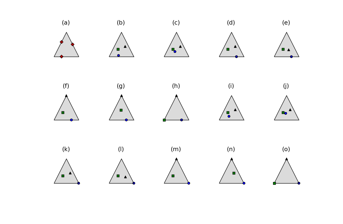
Figure 3: We are given an instance of a partial label problem where M=L=3M=L=3 and the partial labels each have two 11s and a single 00. In (a), the red diamonds represent the mixture proportions of the distributions P~1,P~2,P~3\tilde{P}_{1},\tilde{P}_{2},\tilde{P}_{3}. In (b), three distributions Q1,Q2,Q3Q_{1},Q_{2},Q_{3} are sampled uniformly randomly from the convex hull of P~1,P~2,P~3\tilde{P}_{1},\tilde{P}_{2},\tilde{P}_{3}; the green square, black triangle, and blue circle represent their mixture proportions. Figures (c)-(h) show how the algorithm generates a set of candidate distributions (W1(2),W2(2),W3(2))T(W^{(2)}_{1},W^{(2)}_{2},W^{(2)}_{3})^{T} with k=2k=2. In (h), PartialLabel runs VertexTest on (W1(2),W2(2),W3(2))T(W^{(2)}_{1},W^{(2)}_{2},W^{(2)}_{3})^{T} and determines that (W1(2),W2(2),W3(2))T(W^{(2)}_{1},W^{(2)}_{2},W^{(2)}_{3})^{T} is not a permutation of (P1,P2,P3)T(P_{1},P_{2},P_{3})^{T}. In (i)-(o), PartialLabel begins again with Q1,Q2,Q3Q_{1},Q_{2},Q_{3} and executes the same series of steps with k=3k=3, generating (W1(3),W2(3),W3(3))T(W^{(3)}_{1},W^{(3)}_{2},W^{(3)}_{3})^{T}. In (o), it runs VertexTest on (W1(3),W2(3),W3(3))T(W^{(3)}_{1},W^{(3)}_{2},W^{(3)}_{3})^{T} and determines that (W1(3),W2(3),W3(3))T(W^{(3)}_{1},W^{(3)}_{2},W^{(3)}_{3})^{T} is a permutation of (P1,P2,P3)T(P_{1},P_{2},P_{3})^{T}.

8.1 Notation

Let AA be a set. A∘A^{\circ} denotes the relative interior of AA, i.e., A∘={x∈A|B⁡(x,r)∩aff⁡A⊆A​ for some ​r>0}A^{\circ}=\{x\in A|B(x,r)\cap\mathop{\text{aff}}A\subseteq A\text{ for some }r>0\}. Then, ∂A\partial A denotes the relative boundary of AA, i.e., ∂A=A∖A∘\partial A=A\setminus A^{\circ}. In addition, let ‖⋅‖\left\|\cdot\right\| denote an arbitrary norm. For two vectors, 𝒙,𝒚∈ℝK\bm{x},\bm{y}\in\mathbb{R}^{K}, define

min⁡(𝒙T,𝒚T)\displaystyle\min(\bm{x}^{T},\bm{y}^{T}) =(min⁡(x1,y1),…,min⁡(xK,yK))\displaystyle=(\min(x_{1},y_{1}),\ldots,\min(x_{K},y_{K}))

We use the following affine mapping throughout the paper: mν​(𝒙,𝒚)=(1−ν)​𝒙+ν​𝒚m_{\nu}(\bm{x},\bm{y})=(1-\nu)\bm{x}+\nu\bm{y} where 𝒙,𝒚∈ℝL\bm{x},\bm{y}\in\mathbb{R}^{L} and ν∈[0,1]\nu\in[0,1]. Overloading notation, when Q1Q_{1} and Q2Q_{2} are distributions, we define mν​(Q1,Q2)=(1−ν)​Q1+ν​Q2m_{\nu}(Q_{1},Q_{2})=(1-\nu)Q_{1}+\nu Q_{2}. We call ν\nu the resampling proportion. Note that if 𝜼1,𝜼2∈ΔL\bm{\eta}_{1},\bm{\eta}_{2}\in\Delta_{L} and Q1=𝜼1T​𝑷Q_{1}=\bm{\eta}_{1}^{T}\bm{P} and Q2=𝜼2T​𝑷Q_{2}=\bm{\eta}_{2}^{T}\bm{P}, then mν​(𝜼1,𝜼2)m_{\nu}(\bm{\eta}_{1},\bm{\eta}_{2}) is the mixture proportion for the distribution mν​(Q1,Q2)m_{\nu}(Q_{1},Q_{2}).

8.2 Necessary Conditions

8.2.1 Mutual Contamination Models

Theorem 1.
(A)

We prove the contrapositive. Let ϕ\phi be a demixing operator and ϕ⁡(𝑷~)=(𝚷,𝑷)\phi(\tilde{\bm{P}})=(\bm{\Pi},\bm{P}). Suppose that there is some PiP_{i} and Q∈conv⁡({Pj:j≠i})Q\in\mathop{\textnormal{conv}}(\{P_{j}:j\neq i\}) with Q=∑j≠iβj​PjQ=\sum_{j\neq i}\beta_{j}P_{j} such that PiP_{i} is not irreducible wrt QQ. Then, there is some distribution GG and γ∈(0,1]\gamma\in(0,1] such that Pi=γ​Q+(1−γ)​GP_{i}=\gamma Q+(1-\gamma)G.

Suppose γ=1\gamma=1. Then, Pi=Q∈conv⁡({Pk:k≠i})P_{i}=Q\in\mathop{\textnormal{conv}}(\{P_{k}:k\neq i\}). But, then P~1,…,P~M∈conv⁡({Pj:j≠i}∪{R})\tilde{P}_{1},\ldots,\tilde{P}_{M}\in\mathop{\textnormal{conv}}(\{P_{j}:j\neq i\}\cup\{R\}) for any distribution R∉conv⁡(P1,…,PL)R\not\in\mathop{\textnormal{conv}}(P_{1},\ldots,P_{L}). This shows that ϕ\phi does not satisfy (M).

Therefore, assume that γ∈(0,1)\gamma\in(0,1). Either G∈conv⁡(P1,…,PL)G\in\mathop{\textnormal{conv}}(P_{1},\ldots,P_{L}) or G∉conv⁡(P1,…,PL)G\not\in\mathop{\textnormal{conv}}(P_{1},\ldots,P_{L}). Suppose that G∈conv⁡(P1,…,PL)G\in\mathop{\textnormal{conv}}(P_{1},\ldots,P_{L}). Then, there exist α1,…,αL\alpha_{1},\ldots,\alpha_{L} all nonnegative and summing to 11 such that

Pi\displaystyle P_{i} =γ​Q+(1−γ)​(α1​P1+…+αL​PL)\displaystyle=\gamma Q+(1-\gamma)(\alpha_{1}P_{1}+\ldots+\alpha_{L}P_{L})

Therefore, Pi∈conv⁡({Pk:k≠i})P_{i}\in\mathop{\textnormal{conv}}(\{P_{k}:k\neq i\}). But then P~1,…,P~M∈conv⁡({Pj:j≠i}∪{R})\tilde{P}_{1},\ldots,\tilde{P}_{M}\in\mathop{\textnormal{conv}}(\{P_{j}:j\neq i\}\cup\{R\}) for any distribution R∉conv⁡(P1,…,PL)R\not\in\mathop{\textnormal{conv}}(P_{1},\ldots,P_{L}). This shows that that ϕ\phi does not satisfy (M).

Now, suppose that G∉conv⁡(P1,…,PL)G\not\in\mathop{\textnormal{conv}}(P_{1},\ldots,P_{L}). Since Pi∈conv⁡(G,Q)P_{i}\in\mathop{\textnormal{conv}}(G,Q) and Q∈conv⁡({Pj:j≠i})Q\in\mathop{\textnormal{conv}}(\{P_{j}:j\neq i\}), we have that conv⁡({Pj:j≠i}∪{G})⊃conv⁡(P1,…,PL)\mathop{\textnormal{conv}}(\{P_{j}:j\neq i\}\cup\{G\})\supset\mathop{\textnormal{conv}}(P_{1},\ldots,P_{L}). Then, P~1,…,P~M∈conv⁡({Pj:j≠i}∪{G})\tilde{P}_{1},\ldots,\tilde{P}_{M}\in\mathop{\textnormal{conv}}(\{P_{j}:j\neq i\}\cup\{G\}). This shows that ϕ\phi does not satisfy (M). The result follows.

(B)

Let ϕ⁡(𝑷~)=(𝚷,𝑷)\phi(\tilde{\bm{P}})=(\bm{\Pi},\bm{P}). Clearly, dimspan⁡(P~1,…,P~M)≤dimspan⁡(P1,…,PL)\dim\mathop{\textnormal{span}}(\tilde{P}_{1},\ldots,\tilde{P}_{M})\leq\dim\mathop{\textnormal{span}}(P_{1},\ldots,P_{L}) since P~i=𝝅iT​𝑷\tilde{P}_{i}=\bm{\pi}_{i}^{T}\bm{P} for all i∈[M]i\in[M]. Since ϕ\phi satisfies (L), span⁡(P1,…,PL)⊂span⁡(P~1,…,P~L)\mathop{\textnormal{span}}(P_{1},\ldots,P_{L})\subset\mathop{\textnormal{span}}(\tilde{P}_{1},\ldots,\tilde{P}_{L}), which implies that dimspan⁡(P1,…,PL)≤dimspan⁡(P~1,…,P~M)\dim\mathop{\textnormal{span}}(P_{1},\ldots,P_{L})\leq\dim\mathop{\textnormal{span}}(\tilde{P}_{1},\ldots,\tilde{P}_{M}). Therefore, dimspan⁡(P~1,…,P~M)=dimspan⁡(P1,…,PL)\dim\mathop{\textnormal{span}}(\tilde{P}_{1},\ldots,\tilde{P}_{M})=\dim\mathop{\textnormal{span}}(P_{1},\ldots,P_{L}). Then, since P~1,…,P~M∈range⁡(𝚷)\tilde{P}_{1},\ldots,\tilde{P}_{M}\in\mathop{\text{range}}(\bm{\Pi}), dimspan⁡(P1,…,PL)≤dimrange⁡𝚷\dim\mathop{\textnormal{span}}(P_{1},\ldots,P_{L})\leq\dim\mathop{\text{range}}\bm{\Pi}. By Result 3.117 of Axler (2015), rank⁡(𝚷)=dimrange​𝚷≥dimspan⁡(P1,…,PL)\mathop{\textnormal{rank}}(\bm{\Pi})=\dim\text{range}\,\bm{\Pi}\geq\dim\mathop{\textnormal{span}}(P_{1},\ldots,P_{L}).

∎

Proposition 2.

Suppose that ϕ⁡(𝑷~)=(𝚷,𝑷)\phi(\tilde{\bm{P}})=(\bm{\Pi},\bm{P}). We first show that ϕ\phi satisfies (L). By hypothesis, P1,…,PLP_{1},\ldots,P_{L} are jointly irreducible. By Lemma B.1 of Blanchard and Scott (2014), P1,…,PLP_{1},\ldots,P_{L} are linearly independent. Since by hypothesis 𝚷\bm{\Pi} has full rank, there exist LL rows in 𝚷\bm{\Pi}, 𝝅i1,…,𝝅iL\bm{\pi}_{i_{1}},\ldots,\bm{\pi}_{i_{L}}, that are linearly independent. By Lemma B.1 of Blanchard and Scott (2014), P~i1,…,P~iL\tilde{P}_{i_{1}},\ldots,\tilde{P}_{i_{L}} are linearly independent. Since 𝚷​𝑷=𝑷~\bm{\Pi}\bm{P}=\tilde{\bm{P}}, span⁡(P~1,…,P~M)⊆span⁡(P1,…,PL)\mathop{\textnormal{span}}(\tilde{P}_{1},\ldots,\tilde{P}_{M})\subseteq\mathop{\textnormal{span}}(P_{1},\ldots,P_{L}). But, then since dimspan⁡(P~1,…,P~M)≥L\dim\mathop{\textnormal{span}}(\tilde{P}_{1},\ldots,\tilde{P}_{M})\geq L, we have span⁡(P~1,…,P~M)=span⁡(P1,…,PL)\mathop{\textnormal{span}}(\tilde{P}_{1},\ldots,\tilde{P}_{M})=\mathop{\textnormal{span}}(P_{1},\ldots,P_{L}). Therefore, ϕ\phi satisfies (L).

Now, we show that ϕ\phi satisfies (M). Suppose that there is another solution (𝚷′,𝑷′)(\bm{\Pi}^{\prime},\bm{P}^{\prime}) with 𝑷′=(P1,…,PL)T\bm{P}^{\prime}=(P_{1},\ldots,P_{L})^{T} such that 𝚷′​𝑷′=𝑷~\bm{\Pi}^{\prime}\bm{P}^{\prime}=\tilde{\bm{P}} and with some Pi′P^{\prime}_{i} such that Pi′∉conv⁡(P1,…,PL)P_{i}^{\prime}\not\in\mathop{\textnormal{conv}}(P_{1},\ldots,P_{L}). We claim that Pi′∉span⁡(P1,…,PL)P_{i}^{\prime}\not\in\mathop{\textnormal{span}}(P_{1},\ldots,P_{L}). If Pi′∈span⁡(P1,…,PL)P_{i}^{\prime}\in\mathop{\textnormal{span}}(P_{1},\ldots,P_{L}), then we must have that Pi′=∑i=1Lai​PiP_{i}^{\prime}=\sum_{i=1}^{L}a_{i}P_{i} where at least one of the aia_{i} is negative. But, by joint irreducibility of P1,…,PLP_{1},\ldots,P_{L}, Pi′P_{i}^{\prime} is not a distribution, which is a contradiction. So, the claim follows. But, then, since span⁡(P1,…,PL)=span⁡(P~1,…,P~M)\mathop{\textnormal{span}}(P_{1},\ldots,P_{L})=\mathop{\textnormal{span}}(\tilde{P}_{1},\ldots,\tilde{P}_{M}), we must have that span⁡(P~1,…,P~M)⊆span⁡(P1′,…,Pi−1′,Pi+1′,…,PL)\mathop{\textnormal{span}}(\tilde{P}_{1},\ldots,\tilde{P}_{M})\subseteq\mathop{\textnormal{span}}(P_{1}^{\prime},\ldots,P_{i-1}^{\prime},P_{i+1}^{\prime},\ldots,P_{L}), which is impossible since dimspan⁡(P~1,…,P~M)=L\dim\mathop{\textnormal{span}}(\tilde{P}_{1},\ldots,\tilde{P}_{M})=L. ∎

8.2.2 Partial Label Model

Definition 6.

A decontamination operator ψ\psi satisfies Maximality (M′) iff ψ⁡(𝐏~,𝐒)=(𝚷,𝐏)\psi(\tilde{\bm{P}},\bm{S})=(\bm{\Pi},\bm{P}) implies that any pair (𝚷′,𝐏′)(\bm{\Pi}^{\prime},\bm{P}^{\prime}) with 𝚷′∈ΔLM\bm{\Pi}^{\prime}\in\Delta_{L}^{M} and 𝐏′=(P1′,…,PL′)T∈𝒫L\bm{P}^{\prime}=(P^{\prime}_{1},\ldots,P^{\prime}_{L})^{T}\in\mathcal{P}^{L} that solves (1) and is consistent with 𝐒\bm{S} is such that {P1′,…,PL′}⊆conv⁡(P1,…,PL)\{P^{\prime}_{1},\ldots,P^{\prime}_{L}\}\subseteq\mathop{\textnormal{conv}}(P_{1},\ldots,P_{L}).

The notion of linearity for a decontamination operator for the partial label model is identical to the notion of linearity for a decontamination operator for a mixed membership model.

Definition 7.

A decontamination operator ψ\psi satisfies Linearity (L′) iff ψ2​(𝐏~,𝐒)=𝐏\psi_{2}(\tilde{\bm{P}},\bm{S})=\bm{P} implies {P1,…,PL}⊆span⁡(P~1,…,P~M)\{P_{1},\ldots,P_{L}\}\subseteq\mathop{\textnormal{span}}(\tilde{P}_{1},\ldots,\tilde{P}_{M}).

Proposition 6.

Let ψ\psi denote a decontamination operator for the partial label model and ψ⁡(𝐏~,𝐒)=(𝚷,𝐏)\psi(\tilde{\bm{P}},\bm{S})=(\bm{\Pi},\bm{P}). (i) If ψ\psi satisfies (L′), then (𝚷,𝐏)(\bm{\Pi},\bm{P}) need not satisfy (A). (ii) If ψ\psi satisfies (L′), then (𝚷,𝐏)(\bm{\Pi},\bm{P}) satisfies (B).

Proof.
(i)

Let Q1∼unif⁡(0,2)Q_{1}\sim\mathop{\text{unif}}(0,2) and Q2∼unif⁡(1,3)Q_{2}\sim\mathop{\text{unif}}(1,3). Let P1=23​Q1+13​Q2P_{1}=\frac{2}{3}Q_{1}+\frac{1}{3}Q_{2}, P2=13​Q1+23​Q2P_{2}=\frac{1}{3}Q_{1}+\frac{2}{3}Q_{2}, P~1=P1\tilde{P}_{1}=P_{1}, and P~2=P2\tilde{P}_{2}=P_{2}. Then, 𝑺=𝑰2\bm{S}=\bm{I}_{2}, identity matrix. Then, any (𝚷′,𝑷′)(\bm{\Pi}^{\prime},\bm{P}^{\prime}) that satisfies (1) and is consistent with 𝑺\bm{S} must be such that (P1,P2)T=𝑷′(P_{1},P_{2})^{T}=\bm{P}^{\prime}. Therefore, (M′) is satisfied. But, clearly, (A) is not satisfied.

(ii)

The proof is identical to the proof that (L) implies (B) for mixed membership models.

∎

Proposition 1.

We give a proof by contraposition. Suppose that there exists i≠ji\neq j such that 𝑺:,i=𝑺:,j\bm{S}_{:,i}=\bm{S}_{:,j}. Without loss of generality, let i=1i=1 and j=2j=2. Suppose that (𝚷,𝑷)(\bm{\Pi},\bm{P}) is consistent with 𝑺\bm{S} and solves 𝑷~=𝚷​𝑷\tilde{\bm{P}}=\bm{\Pi}\bm{P}. Then, the pair (𝚷′,𝑷′)(\bm{\Pi}^{\prime},\bm{P}^{\prime})

𝚷′=\displaystyle\bm{\Pi}^{\prime}= (𝚷:,2𝚷:,1𝚷:,3…𝚷:,L)\displaystyle\begin{pmatrix}\bm{\Pi}_{:,2}&\bm{\Pi}_{:,1}&\bm{\Pi}_{:,3}&\ldots&\bm{\Pi}_{:,L}\end{pmatrix}
𝑷′\displaystyle\bm{P}^{\prime} =(P2P1P3PL)\displaystyle=\begin{pmatrix}P_{2}\\ P_{1}\\ P_{3}\\ \vdots\\ P_{L}\\ \end{pmatrix}

solves 𝑷~=𝚷′​𝑷′\tilde{\bm{P}}=\bm{\Pi}^{\prime}\bm{P}^{\prime} and is consistent with 𝑺\bm{S}. ∎

Proposition 7.

If a decontamination operator ψ\psi is such that ψ⁡((,,,))=(𝚷,𝐏)\psi((\tilde{\bm{P}},\bm{S}))=(\bm{\Pi},\bm{P}) only if (𝚷,𝐏)(\bm{\Pi},\bm{P}) satisfy (A′) and (B′), then ϕ\phi satisfies (L).

Proof.

The proof is identical to the first paragraph of the proof of Proposition 2. ∎

8.3 Residue Algorithms

Algorithm 4 Residue(F0|F1F_{0}\,|\,F_{1})
1:  κ⟵κ∗​(F0|F1)\kappa\longleftarrow\kappa^{*}(F_{0}\,|\,F_{1})
2:  return F0−κ⁡(1−F1)1−κ\frac{F_{0}-\kappa(1-F_{1})}{1-\kappa}
Algorithm 5 Residue(F0|{F1,…,FK}F_{0}\,|\,\{F_{1},\ldots,F_{K}\})
1:  (ν1,…,νK)⟵(ν1′,…,νK′)​ achieving the maximum in ​κ∗​(F0|F1,…,FK)(\nu_{1},\ldots,\nu_{K})\longleftarrow(\nu^{\prime}_{1},\ldots,\nu^{\prime}_{K})\text{ achieving the maximum in }\kappa^{*}(F_{0}\,|\,F_{1},\ldots,F_{K})
2:  return F0−∑i=1Kνi​Fi1−∑i=1Kνi\frac{F_{0}-\sum_{i=1}^{K}\nu_{i}F_{i}}{1-\sum_{i=1}^{K}\nu_{i}}

8.4 General Lemmas

Prop 4.

Without loss of generality, suppose l=1l=1 and let A=[L]∖{1}A=[L]\setminus\{1\}; the other cases follow by a similar argument. Suppose GG is such that

Q1\displaystyle Q_{1} =(1−∑j≥2μj)​G+∑j≥2μj​Qj\displaystyle=(1-\sum_{j\geq 2}\mu_{j})G+\sum_{j\geq 2}\mu_{j}Q_{j}

Note that since 𝜼1,…,𝜼L\bm{\eta}_{1},\ldots,\bm{\eta}_{L} are linearly independent and P1,…,PLP_{1},\ldots,P_{L} are jointly irreducible, Q1,…,QLQ_{1},\ldots,Q_{L} are linearly independent by Lemma B.1 from Blanchard and Scott (2014). Therefore, ∑j≥2μj<1\sum_{j\geq 2}\mu_{j}<1 because, if not, Q1=∑j≥2μj​QjQ_{1}=\sum_{j\geq 2}\mu_{j}Q_{j}. Therefore, κ∗​(Q1|{Qj:j≠1})<1\kappa^{*}(Q_{1}\,|\,\{Q_{j}:j\neq 1\})<1.

Further, any GG that satisfies the above equation has the form ∑i=1Lγi​Pi\sum_{i=1}^{L}\gamma_{i}P_{i}. The γi\gamma_{i} must sum to one, and we have that they are nonnegative by joint irreducibility. That is, 𝜸≡(γ1,…,γL)T\bm{\gamma}\equiv\begin{pmatrix}\gamma_{1},\ldots,\gamma_{L}\end{pmatrix}^{T} is a discrete distribution. Then, the above equation is equivalent to

𝜼1T​𝑷\displaystyle\bm{\eta}^{T}_{1}\bm{P} =(1−∑j≥2μj)​𝜸T​𝑷+∑j≥2μj​𝜼jT​𝑷\displaystyle=(1-\sum_{j\geq 2}\mu_{j})\bm{\gamma}^{T}\bm{P}+\sum_{j\geq 2}\mu_{j}\bm{\eta}_{j}^{T}\bm{P}

Since P1,…,PLP_{1},\ldots,P_{L} are jointly irreducible, P1,…,PLP_{1},\ldots,P_{L} are linearly independent by Lemma B.1 Blanchard and Scott (2014). By linear independence of P1,…,PLP_{1},\ldots,P_{L}, we obtain

𝜼1\displaystyle\bm{\eta}_{1} =(1−∑j≥2μj)​𝜸+∑j≥2μj​𝜼j\displaystyle=(1-\sum_{j\geq 2}\mu_{j})\bm{\gamma}+\sum_{j\geq 2}\mu_{j}\bm{\eta}_{j}

Consequently, κ∗​(Q1|{Qj:j≠1})=κ∗​(𝜼1|{𝜼j:j≠1})<1\kappa^{*}(Q_{1}\,|\,\{Q_{j}:j\neq 1\})=\kappa^{*}(\bm{\eta}_{1}\,|\,\{\bm{\eta}_{j}:j\neq 1\})<1 and there is a one-to-one correspondence between the feasible solution in κ∗​(Q1|{Qj:j≠1})\kappa^{*}(Q_{1}\,|\,\{Q_{j}:j\neq 1\}) and the feasible solution in κ∗​(𝜼1|{𝜼j:j≠1})\kappa^{*}(\bm{\eta}_{1}\,|\,\{\bm{\eta}_{j}:j\neq 1\}). The one-to-one correspondence is given by G=𝜸T​𝑷G=\bm{\gamma}^{T}\bm{P}.

There is at least one point attaining the maximum in the optimization problem κ∗​(𝜼1|{𝜼j:j≠1})\kappa^{*}(\bm{\eta}_{1}\,|\,\{\bm{\eta}_{j}:j\neq 1\}) by Lemma A.1 in Blanchard and Scott (2014).

We see that the maximizing μj\mu_{j} are unique as follows. Suppose

Q1=(1−κ∗)​G+∑j≥2μj​Qj=(1−κ∗)​G+∑j≥2μj′​Qj\displaystyle Q_{1}=(1-\kappa^{*})G+\sum_{j\geq 2}\mu_{j}Q_{j}=(1-\kappa^{*})G+\sum_{j\geq 2}\mu_{j}^{\prime}Q_{j}

The linear independence of Q1,…,QLQ_{1},\ldots,Q_{L} implies that μj=μj′\mu_{j}=\mu_{j}^{\prime}. ∎

Lemma 1 gives us some useful properties of the two-sample κ∗\kappa^{*} that we exploit in the PartialLabel and Demix algorithms. Statement 1 gives an alternative form of κ∗\kappa^{*}. Statement 2 gives the intuitive result that the residues lie on the boundary of the simplex. Statement 3 gives a useful relation for determining whether two mixture proportions are on the same face; we use this relation extensively in our algorithms.

Lemma 1.

Let F1,…,FKF_{1},\ldots,F_{K} be jointly irreducible distributions with 𝐅=(F1,…,FK)T\bm{F}=(F_{1},\ldots,F_{K})^{T}, Q1,Q2Q_{1},Q_{2} be two distributions such that Qi=𝛈iT​𝐅Q_{i}=\bm{\eta}_{i}^{T}\bm{F} where 𝛈i∈ΔK\bm{\eta}_{i}\in\Delta_{K} for i=1,2i=1,2 and 𝛈1≠𝛈2\bm{\eta}_{1}\neq\bm{\eta}_{2}. Let RR be the residue of Q1Q_{1} wrt Q2Q_{2} and R=𝛍T​𝐅R=\bm{\mu}^{T}\bm{F}.

  1. 1.

    We have the following equivalence of optimization problems:

    κ∗​(Q1|Q2)\displaystyle\kappa^{*}(Q_{1}\,|\,Q_{2}) =max⁡(α≥1|∃ a distribution ​G​ s.t ​G=Q2+α⁡(Q1−Q2))\displaystyle=\max(\alpha\geq 1|\exists\text{ a distribution }G\text{ s.t }G=Q_{2}+\alpha(Q_{1}-Q_{2}))
  2. 2.

    𝝁∈∂ΔK\bm{\mu}\in\partial\Delta_{K}.

  3. 3.

    𝒮⁡(𝜼2)⊈𝒮⁡(𝜼1)\mathcal{S}(\bm{\eta}_{2})\not\subseteq\mathcal{S}(\bm{\eta}_{1}) if and only if R=Q1R=Q_{1} if and only if κ∗​(Q1|Q2)=0\kappa^{*}(Q_{1}\,|\,Q_{2})=0.

Lemma 1.
  1. 1.

    Consider the linear relation: Q1=(1−κ)​G+κ​Q2Q_{1}=(1-\kappa)G+\kappa Q_{2} where κ∈[0,1]\kappa\in[0,1]. Since F1,…,FKF_{1},\ldots,F_{K} are jointly irreducible and 𝜼1\bm{\eta}_{1} and 𝜼2\bm{\eta}_{2} are linearly independent, Q1Q_{1} and Q2Q_{2} are linearly independent by Lemma B.1 of Blanchard and Scott (2014). Therefore, κ<1\kappa<1. We can rewrite the relation as follows:

    G=11−κ​Q1−κ1−κ​Q2=α​Q1+(1−α)​Q2\displaystyle G=\frac{1}{1-\kappa}Q_{1}-\frac{\kappa}{1-\kappa}Q_{2}=\alpha Q_{1}+(1-\alpha)Q_{2}

    where α=11−κ\alpha=\frac{1}{1-\kappa}. The equivalence follows.

  2. 2.

    Since RR is the residue of Q1Q_{1} wrt Q2Q_{2}, by Proposition 4, 𝝁\bm{\mu} is the residue of 𝜼1\bm{\eta}_{1} wrt 𝜼2\bm{\eta}_{2} and 𝝁∈ΔK\bm{\mu}\in\Delta_{K}. Therefore, by statement 1 in Lemma 1, 𝝁\bm{\mu} is such that α∗\alpha^{*} is maximized subject to the following constraints:

    𝝁\displaystyle\bm{\mu} =(1−α∗)​𝜼2+α∗​𝜼1\displaystyle=(1-\alpha^{*})\bm{\eta}_{2}+\alpha^{*}\bm{\eta}_{1}
    α∗\displaystyle\alpha^{*} ≥1\displaystyle\geq 1
    𝝁\displaystyle\bm{\mu} ∈ΔK\displaystyle\in\Delta_{K}

    Suppose that mini⁡μi>0\min_{i}\mu_{i}>0. Then, there is some ϵ>0\epsilon>0 such that

    𝝁′\displaystyle\bm{\mu}^{\prime} =(1−α∗−ϵ)​𝜼2+(α∗+ϵ)​𝜼1\displaystyle=(1-\alpha^{*}-\epsilon)\bm{\eta}_{2}+(\alpha^{*}+\epsilon)\bm{\eta}_{1}
    α∗+ϵ\displaystyle\alpha^{*}+\epsilon ≥1\displaystyle\geq 1
    𝝁′\displaystyle\bm{\mu}^{\prime} ∈ΔK\displaystyle\in\Delta_{K}

    But, this contradicts the definition of α∗\alpha^{*} and 𝝁\bm{\mu}. Therefore, mini⁡μi=0\min_{i}\mu_{i}=0. Consequently, 𝝁∈∂ΔK\bm{\mu}\in\partial\Delta_{K}.

  3. 3.

    By definition of κ∗\kappa^{*}, it is clear that R=Q1R=Q_{1} if and only if κ∗​(Q1|Q2)=0\kappa^{*}(Q_{1}\,|\,Q_{2})=0. Therefore, it suffices to show that 𝒮⁡(𝜼2)⊈𝒮⁡(𝜼1)\mathcal{S}(\bm{\eta}_{2})\not\subseteq\mathcal{S}(\bm{\eta}_{1}) if and only if κ∗​(Q1|Q2)=0\kappa^{*}(Q_{1}\,|\,Q_{2})=0. Suppose 𝒮⁡(𝜼2)⊈𝒮⁡(𝜼1)\mathcal{S}(\bm{\eta}_{2})\not\subseteq\mathcal{S}(\bm{\eta}_{1}). Then, there must be i∈[K]i\in[K] such that η2,i>0\eta_{2,i}>0 and η1,i=0\eta_{1,i}=0. Then, for α>1\alpha>1,

    mini∈[K]⁡(1−α)​η2,i+α​η1,i<0\displaystyle\min_{i\in[K]}(1-\alpha)\eta_{2,i}+\alpha\eta_{1,i}<0

    But, this violates the constraint of the optimization problem. Therefore, α=1\alpha=1. By statement 1 in Lemma 1, κ∗​(𝜼1|𝜼2)=0\kappa^{*}(\bm{\eta}_{1}\,|\,\bm{\eta}_{2})=0. By Proposition 4, κ∗​(Q1|Q2)=κ∗​(𝜼1|𝜼2)=0\kappa^{*}(Q_{1}\,|\,Q_{2})=\kappa^{*}(\bm{\eta}_{1}\,|\,\bm{\eta}_{2})=0.

    Now, suppose 𝒮⁡(𝜼2)⊆𝒮⁡(𝜼1)\mathcal{S}(\bm{\eta}_{2})\subseteq\mathcal{S}(\bm{\eta}_{1}). Then, for any i∈[K]i\in[K], if η2,i>0\eta_{2,i}>0, then η1,i>0\eta_{1,i}>0. Then, there is α>1\alpha>1 sufficiently close to 11 such that

    mini∈[K]⁡η2,i+α⁡(η1,i−η2,i)≥0\displaystyle\min_{i\in[K]}\eta_{2,i}+\alpha(\eta_{1,i}-\eta_{2,i})\geq 0

    By statement 1 in this Lemma, κ∗​(𝜼1|𝜼2)>0\kappa^{*}(\bm{\eta}_{1}\,|\,\bm{\eta}_{2})>0. By proposition 4, κ∗​(Q1|Q2)=κ∗​(𝜼1|𝜼2)>0\kappa^{*}(Q_{1}\,|\,Q_{2})=\kappa^{*}(\bm{\eta}_{1}\,|\,\bm{\eta}_{2})>0.

∎

8.5 Demixing Mixed Membership Models

8.5.1 Lemmas

Lemma 2 establishes an intuitive continuity property of the two-sample version of κ∗\kappa^{*} and the residue.

Lemma 2.

Let 𝛈1,𝛈2,𝛈3∈ΔL\bm{\eta}_{1},\bm{\eta}_{2},\bm{\eta}_{3}\in\Delta_{L} be distinct vectors and let 𝛍\bm{\mu} be the residue of 𝛈2\bm{\eta}_{2} wrt 𝛈1\bm{\eta}_{1}. Let αn\alpha_{n} be a sequence such that αn⟶1\alpha_{n}\longrightarrow 1 as n⟶∞n\longrightarrow\infty and let 𝛕n\bm{\tau}_{n} be the residue of αn​𝛈2+(1−αn)​𝛈3\alpha_{n}\bm{\eta}_{2}+(1-\alpha_{n})\bm{\eta}_{3} wrt 𝛈1\bm{\eta}_{1}. Then,

  1. 1.

    limn⟶∞κ∗​(αn​𝜼2+(1−αn)​𝜼3|𝜼1)=κ∗​(𝜼2|𝜼1)\lim_{n\longrightarrow\infty}\kappa^{*}(\alpha_{n}\bm{\eta}_{2}+(1-\alpha_{n})\bm{\eta}_{3}\,|\,\bm{\eta}_{1})=\kappa^{*}(\bm{\eta}_{2}\,|\,\bm{\eta}_{1})

  2. 2.

    limn⟶∞‖𝝉n−𝝁‖=0\lim_{n\longrightarrow\infty}\left\|\bm{\tau}_{n}-\bm{\mu}\right\|=0

Lemma 2.
  1. 1.

    In order to apply the residue operator κ∗\kappa^{*} to 𝜼1,𝜼2,𝜼3\bm{\eta}_{1},\bm{\eta}_{2},\bm{\eta}_{3}, we think of 𝜼1,𝜼2,𝜼3\bm{\eta}_{1},\bm{\eta}_{2},\bm{\eta}_{3} as discrete probability distributions. Let (𝒳,𝒞)(\mathcal{X},\mathcal{C}) be the measurable space on which 𝜼1,𝜼2,𝜼3\bm{\eta}_{1},\bm{\eta}_{2},\bm{\eta}_{3} are defined. Note that 𝒳\mathcal{X} is finite and let 𝒞=2𝒳\mathcal{C}=2^{\mathcal{X}} (i.e., the power set of 𝒳\mathcal{X}), which is also finite. By Proposition 1 of Blanchard and Scott (2014),

    κ∗​(𝜼2|𝜼1)\displaystyle\kappa^{*}(\bm{\eta}_{2}\,|\,\bm{\eta}_{1}) =infC∈𝒞,𝜼1​(C)>0𝜼2​(C)𝜼1​(C)\displaystyle=\inf_{C\in\mathcal{C},\bm{\eta}_{1}(C)>0}\frac{\bm{\eta}_{2}(C)}{\bm{\eta}_{1}(C)}

    Since 𝒞\mathcal{C} is finite, there is ϵ>0\epsilon>0 such that infC∈𝒞,𝜼1​(C)>0𝜼1​(C)>ϵ\inf_{C\in\mathcal{C},\bm{\eta}_{1}(C)>0}\bm{\eta}_{1}(C)>\epsilon. Then,

    κ∗​(αn​𝜼2+(1−αn)​𝜼3|𝜼1)\displaystyle\kappa^{*}(\alpha_{n}\bm{\eta}_{2}+(1-\alpha_{n})\bm{\eta}_{3}\,|\,\bm{\eta}_{1}) =infC∈𝒞,𝜼1​(C)>0αn​𝜼2​(C)+(1−αn)​𝜼3​(C)𝜼1​(C)\displaystyle=\inf_{C\in\mathcal{C},\bm{\eta}_{1}(C)>0}\frac{\alpha_{n}\bm{\eta}_{2}(C)+(1-\alpha_{n})\bm{\eta}_{3}(C)}{\bm{\eta}_{1}(C)}
    ≤αn​infC∈𝒞,𝜼1​(C)>0𝜼2​(C)𝜼1​(C)+1−αnϵ\displaystyle\leq\alpha_{n}\inf_{C\in\mathcal{C},\bm{\eta}_{1}(C)>0}\frac{\bm{\eta}_{2}(C)}{\bm{\eta}_{1}(C)}+\frac{1-\alpha_{n}}{\epsilon}
    ⟶infC∈𝒞,𝜼1​(C)>0𝜼2​(C)𝜼1​(C)\displaystyle\longrightarrow\inf_{C\in\mathcal{C},\bm{\eta}_{1}(C)>0}\frac{\bm{\eta}_{2}(C)}{\bm{\eta}_{1}(C)}

    as n⟶∞n\longrightarrow\infty. Further, since 𝜼2​(⋅)𝜼1​(⋅)\frac{\bm{\eta}_{2}(\cdot)}{\bm{\eta}_{1}(\cdot)} and 𝜼3​(⋅)𝜼1​(⋅)\frac{\bm{\eta}_{3}(\cdot)}{\bm{\eta}_{1}(\cdot)} are bounded over {C∈𝒞:𝜼1​(C)>0}\{C\in\mathcal{C}:\bm{\eta}_{1}(C)>0\},

    κ∗​(αn​𝜼2+(1−αn)​𝜼3|𝜼1)\displaystyle\kappa^{*}(\alpha_{n}\bm{\eta}_{2}+(1-\alpha_{n})\bm{\eta}_{3}\,|\,\bm{\eta}_{1}) =infC∈𝒞,𝜼1​(C)>0αn​𝜼2​(C)+(1−αn)​𝜼3​(C)𝜼1​(C)\displaystyle=\inf_{C\in\mathcal{C},\bm{\eta}_{1}(C)>0}\frac{\alpha_{n}\bm{\eta}_{2}(C)+(1-\alpha_{n})\bm{\eta}_{3}(C)}{\bm{\eta}_{1}(C)}
    ≥αn​infC∈𝒞,𝜼1​(C)>0𝜼2​(C)𝜼1​(C)+(1−αn)​infC∈𝒞,𝜼1​(C)>0𝜼3​(C)𝜼1​(C)\displaystyle\geq\alpha_{n}\inf_{C\in\mathcal{C},\bm{\eta}_{1}(C)>0}\frac{\bm{\eta}_{2}(C)}{\bm{\eta}_{1}(C)}+(1-\alpha_{n})\inf_{C\in\mathcal{C},\bm{\eta}_{1}(C)>0}\frac{\bm{\eta}_{3}(C)}{\bm{\eta}_{1}(C)}
    ⟶infC∈𝒞,𝜼1​(C)>0𝜼2​(C)𝜼1​(C)\displaystyle\longrightarrow\inf_{C\in\mathcal{C},\bm{\eta}_{1}(C)>0}\frac{\bm{\eta}_{2}(C)}{\bm{\eta}_{1}(C)}

    as n⟶∞n\longrightarrow\infty. By the sandwich principle of limits, the result follows.

  2. 2.

    We write 𝝁=κ​𝜼2+(1−κ)​𝜼1\bm{\mu}=\kappa\bm{\eta}_{2}+(1-\kappa)\bm{\eta}_{1} and 𝝉n=κn​(αn​𝜼2+(1−αn)​𝜼3)+(1−κn)​𝜼1\bm{\tau}_{n}=\kappa_{n}(\alpha_{n}\bm{\eta}_{2}+(1-\alpha_{n})\bm{\eta}_{3})+(1-\kappa_{n})\bm{\eta}_{1} where κ=κ∗​(𝜼2|𝜼1)\kappa=\kappa^{*}(\bm{\eta}_{2}\,|\,\bm{\eta}_{1}) and κn=κ∗​(αn​𝜼2+(1−αn)​𝜼3|𝜼1)\kappa_{n}=\kappa^{*}(\alpha_{n}\bm{\eta}_{2}+(1-\alpha_{n})\bm{\eta}_{3}\,|\,\bm{\eta}_{1}). Then, by the triangle inequality,

    ‖𝝁−𝝉n‖\displaystyle\left\|\bm{\mu}-\bm{\tau}_{n}\right\| =‖(κn−κ)​𝜼1+(κ−κn​αn)​𝜼2−(1−αn)​𝜼3‖\displaystyle=\left\|(\kappa_{n}-\kappa)\bm{\eta}_{1}+(\kappa-\kappa_{n}\alpha_{n})\bm{\eta}_{2}-(1-\alpha_{n})\bm{\eta}_{3}\right\|
    ≤|κn−κ​|‖𝜼1‖+|​κ−κn​αn|‖𝜼2‖+|1−αn|​‖𝜼3‖\displaystyle\leq|\kappa_{n}-\kappa|\left\|\bm{\eta}_{1}\right\|+|\kappa-\kappa_{n}\alpha_{n}|\left\|\bm{\eta}_{2}\right\|+|1-\alpha_{n}|\left\|\bm{\eta}_{3}\right\|
    ⟶0\displaystyle\longrightarrow 0

    as n⟶∞n\longrightarrow\infty since αn⟶1\alpha_{n}\longrightarrow 1 and κn⟶κ\kappa_{n}\longrightarrow\kappa by statement 1 in Lemma 2.

∎

Lemma 3 guarantees that certain operations in the Demix algorithm preserve linear independence of the mixture proportions.

Lemma 3.

Let 𝛕1,…,𝛕K∈ΔL\bm{\tau}_{1},\ldots,\bm{\tau}_{K}\in\Delta_{L} be linearly independent and P1,…,PLP_{1},\ldots,P_{L} be jointly irreducible. Let Qi=𝛕iT​𝐏Q_{i}=\bm{\tau}_{i}^{T}\bm{P} for i∈[K]i\in[K]. Then for any i,j∈[K]i,j\in[K] such that i≠ji\neq j,

  1. 1.

    If 𝜼=∑k=1Kak​𝝉k\bm{\eta}=\sum_{k=1}^{K}a_{k}\bm{\tau}_{k} with aj≠0a_{j}\neq 0, then 𝝉1,…,𝝉j−1,𝜼,𝝉j+1,…,𝝉K\bm{\tau}_{1},\ldots,\bm{\tau}_{j-1},\bm{\eta},\bm{\tau}_{j+1},\ldots,\bm{\tau}_{K} are linearly independent.

  2. 2.

    Let RkR_{k} be the residue of QkQ_{k} with respect to QjQ_{j} for all k∈[K]∖{j}k\in[K]\setminus\{j\}. Then, Rk=𝜼kT​𝑷R_{k}=\bm{\eta}^{T}_{k}\bm{P} where 𝜼k∈ΔK\bm{\eta}_{k}\in\Delta_{K} and 𝜼1,…,𝜼j−1,𝝉j,𝜼j+1,…,𝜼K\bm{\eta}_{1},\ldots,\bm{\eta}_{j-1},\bm{\tau}_{j},\bm{\eta}_{j+1},\ldots,\bm{\eta}_{K} are linearly independent.

  3. 3.

    Let 𝝉∗∈conv⁡(𝝉1,…,𝝉k)∘\bm{\tau}^{*}\in\mathop{\textnormal{conv}}(\bm{\tau}_{1},\ldots,\bm{\tau}_{k})^{\circ} and 𝜼i∈conv⁡(𝝉i,𝝉∗)∘\bm{\eta}_{i}\in\mathop{\textnormal{conv}}(\bm{\tau}_{i},\bm{\tau}^{*})^{\circ} for i∈[k]i\in[k] where k≤Kk\leq K. Then,

    𝜼1,𝜼2,…,𝜼k,𝝉k+1,…,𝝉K\displaystyle\bm{\eta}_{1},\bm{\eta}_{2},\ldots,\bm{\eta}_{k},\bm{\tau}_{k+1},\ldots,\bm{\tau}_{K}

    are linearly independent.

Lemma 3.
  1. 1.

    Let 𝜼=∑k=1Kak​𝝉k\bm{\eta}=\sum_{k=1}^{K}a_{k}\bm{\tau}_{k} with aj≠0a_{j}\neq 0 for some j∈[K]j\in[K]. Let b1,…,bK∈ℝb_{1},\ldots,b_{K}\in\mathbb{R} such that

    0\displaystyle 0 =b1​𝝉1+…+bj−1​𝝉j−1+bj​𝜼+bj+1​𝝉j+1+…+bK​𝝉K\displaystyle=b_{1}\bm{\tau}_{1}+\ldots+b_{j-1}\bm{\tau}_{j-1}+b_{j}\bm{\eta}+b_{j+1}\bm{\tau}_{j+1}+\ldots+b_{K}\bm{\tau}_{K}
    =(b1+bj​a1)​𝝉1+…+(bj−1+bj​aj−1)​𝝉j−1+bj​aj​𝝉j+\displaystyle=(b_{1}+b_{j}a_{1})\bm{\tau}_{1}+\ldots+(b_{j-1}+b_{j}a_{j-1})\bm{\tau}_{j-1}+b_{j}a_{j}\bm{\tau}_{j}+
    (bj+1+bj​aj+1)​𝝉j+1+…+(bK+bj​aK)​𝝉K\displaystyle(b_{j+1}+b_{j}a_{j+1})\bm{\tau}_{j+1}+\ldots+(b_{K}+b_{j}a_{K})\bm{\tau}_{K}

    Since 𝝉1,…,𝝉K\bm{\tau}_{1},\ldots,\bm{\tau}_{K} are linearly independent, bj​aj=0b_{j}a_{j}=0. Since aj≠0a_{j}\neq 0 by hypothesis, bj=0b_{j}=0. Therefore, the previous equation reduces to

    b1​𝝉1+…+bj−1​𝝉j−1+bj+1​𝝉j+1+…+bK​𝝉K\displaystyle b_{1}\bm{\tau}_{1}+\ldots+b_{j-1}\bm{\tau}_{j-1}+b_{j+1}\bm{\tau}_{j+1}+\ldots+b_{K}\bm{\tau}_{K} =0\displaystyle=0

    By the linear independence of 𝝉1,…,𝝉K\bm{\tau}_{1},\ldots,\bm{\tau}_{K}, b1=…=bK=0b_{1}=\ldots=b_{K}=0. The result follows.

  2. 2.

    Let k∈[K]∖{j}k\in[K]\setminus\{j\}. By Proposition 4, 𝜼k\bm{\eta}_{k} is the residue of 𝝉k\bm{\tau}_{k} with respect to 𝝉j\bm{\tau}_{j} and 𝜼k∈ΔL\bm{\eta}_{k}\in\Delta_{L}. By statement 1 of Lemma 1, there is αk≥1\alpha_{k}\geq 1 such that 𝜼k=(1−αk)​𝝉j+α​𝝉k\bm{\eta}_{k}=(1-\alpha_{k})\bm{\tau}_{j}+\alpha\bm{\tau}_{k}. By statement 1 of Lemma 3, 𝜼1,𝝉2,…,𝝉k\bm{\eta}_{1},\bm{\tau}_{2},\ldots,\bm{\tau}_{k} are linearly independent. Using induction and statement 1 of 3, 𝜼1,…,𝜼j−1,𝝉j,𝜼j+1,…,𝜼k\bm{\eta}_{1},\ldots,\bm{\eta}_{j-1},\bm{\tau}_{j},\bm{\eta}_{j+1},\ldots,\bm{\eta}_{k} are linearly independent.

  3. 3.

    We show the result inductively. By statement 1 of Lemma 3, it follows immediately that 𝜼1,𝝉2,…,𝝉K\bm{\eta}_{1},\bm{\tau}_{2},\ldots,\bm{\tau}_{K} are linearly independent. Now, suppose 𝜼1,…,𝜼k−1,𝝉k,…,𝝉K\bm{\eta}_{1},\ldots,\bm{\eta}_{k-1},\bm{\tau}_{k},\ldots,\bm{\tau}_{K} are linearly independent. Then, there exist unique α1,…,αK\alpha_{1},\ldots,\alpha_{K} such that 𝝉∗=∑i=1k−1αi​𝜼i+∑i=kKαi​𝝉i\bm{\tau}^{*}=\sum_{i=1}^{k-1}\alpha_{i}\bm{\eta}_{i}+\sum_{i=k}^{K}\alpha_{i}\bm{\tau}_{i}. Further, since 𝜼k∈conv⁡(𝝉j,𝝉∗)∘\bm{\eta}_{k}\in\mathop{\textnormal{conv}}(\bm{\tau}_{j},\bm{\tau}^{*})^{\circ}, there exists β∈(0,1)\beta\in(0,1) such that 𝜼k=β⁡(∑i=1k−1αi​𝜼i+∑i=kKαi​𝝉i)+(1−β)​𝝉k\bm{\eta}_{k}=\beta(\sum_{i=1}^{k-1}\alpha_{i}\bm{\eta}_{i}+\sum_{i=k}^{K}\alpha_{i}\bm{\tau}_{i})+(1-\beta)\bm{\tau}_{k}. By statement 1 of Lemma 3, it suffices to show that β​αk+(1−β)≠0\beta\alpha_{k}+(1-\beta)\neq 0. Suppose to the contrary that β​αk+(1−β)=0\beta\alpha_{k}+(1-\beta)=0. Then, αk=1−1β<0\alpha_{k}=1-\frac{1}{\beta}<0. So, it is enough to show that 𝝉∗∈conv⁡(𝜼1,…,𝜼k,𝝉k+1,…,𝝉K)\bm{\tau}^{*}\in\mathop{\textnormal{conv}}(\bm{\eta}_{1},\ldots,\bm{\eta}_{k},\bm{\tau}_{k+1},\ldots,\bm{\tau}_{K}).

    We prove the claim inductively. By Statement 1 of 3, 𝜼1,𝝉2,…,𝝉K\bm{\eta}_{1},\bm{\tau}_{2},\ldots,\bm{\tau}_{K} are linearly independent, so there exists unique c1,…,cKc_{1},\ldots,c_{K} such that 𝝉∗=c1​𝜼1+∑i=2Kci​𝝉i\bm{\tau}^{*}=c_{1}\bm{\eta}_{1}+\sum_{i=2}^{K}c_{i}\bm{\tau}_{i}. Since 𝜼1∈conv⁡(𝝉1,𝝉∗)\bm{\eta}_{1}\in\mathop{\textnormal{conv}}(\bm{\tau}_{1},\bm{\tau}^{*}), there exists γ∈(0,1)\gamma\in(0,1) such that c1​(γ​𝝉1+(1−γ)​𝝉∗)+∑i=2Kci​𝝉i=𝝉∗c_{1}(\gamma\bm{\tau}_{1}+(1-\gamma)\bm{\tau}^{*})+\sum_{i=2}^{K}c_{i}\bm{\tau}_{i}=\bm{\tau}^{*}. If c1<0c_{1}<0, then 𝝉∗∉conv⁡(𝝉1,…,𝝉K)\bm{\tau}^{*}\not\in\mathop{\textnormal{conv}}(\bm{\tau}_{1},\ldots,\bm{\tau}_{K}), which is a contradiction. The claim follows inductively.

    Having established the claim, the result follows.

∎

Lemma 4 establishes that the operation performed in the last for loop at the end of the Demix algorithm gives the desired distribution.

Lemma 4.

Let P1,…,PLP_{1},\ldots,P_{L} be jointly irreducible, (Q1,…,QK−1)(Q_{1},\ldots,Q_{K-1}) be a permutation of (Pi1,…,PiK−1)(P_{i_{1}},\ldots,P_{i_{K-1}}) and QK1∈conv⁡(Pi1,…,PiK)∘Q^{1}_{K}\in\mathop{\textnormal{conv}}(P_{i_{1}},\ldots,P_{i_{K}})^{\circ}. Define the sequence

QKi\displaystyle Q_{K}^{i} ⟵Residue​(QKi−1|Qi−1)\displaystyle\longleftarrow\text{Residue}(Q_{K}^{i-1}\,|\,Q_{i-1})

Then, QKK=PiKQ_{K}^{K}=P_{i_{K}}.

Lemma 4.

Relabel the distributions so that Qj=PjQ_{j}=P_{j}. Let 𝝁1\bm{\mu}_{1} denote the mixture proportion of QK1Q_{K}^{1} and 𝒆j\bm{e}_{j} the mixture proportion of PjP_{j}. Consider the sequence given by

𝝁i\displaystyle\bm{\mu}_{i} ⟵Residue​(𝝁i−1|𝒆i−1)\displaystyle\longleftarrow\text{Residue}(\bm{\mu}_{i-1}\,|\,\bm{e}_{i-1})

We claim that 𝝁i,𝒆1,…,𝒆K−1\bm{\mu}_{i},\bm{e}_{1},\ldots,\bm{e}_{K-1} are linearly independent and 𝝁i\bm{\mu}_{i} is the mixture proportion of 𝑸Ki\bm{Q}_{K}^{i}. We prove it inductively. The base case is clear by the hypothesis. Suppose that 𝝁n,𝒆1,…,𝒆K−1\bm{\mu}_{n},\bm{e}_{1},\ldots,\bm{e}_{K-1} are linearly independent and 𝝁n\bm{\mu}_{n} is the mixture proportion of QKnQ_{K}^{n}. Since P1,…,PLP_{1},\ldots,P_{L} are jointly irreducible, by Proposition 4, Residue​(𝝁n|𝒆n)\text{Residue}(\bm{\mu}_{n}\,|\,\bm{e}_{n}) gives the mixture proportion of Q2n+1Q_{2}^{n+1}. By statement 1 of Lemma 3, for any α≥1\alpha\geq 1 α​𝝁n+(1−α)​𝒆n,𝒆1,…,𝒆K−1\alpha\bm{\mu}_{n}+(1-\alpha)\bm{e}_{n},\bm{e}_{1},\ldots,\bm{e}_{K-1} is linearly independent. Therefore, in particular, by statement 11 of Lemma 1, Residue​(𝝁n|𝒆n),𝒆1,…,𝒆K−1\text{Residue}(\bm{\mu}_{n}\,|\,\bm{e}_{n}),\bm{e}_{1},\ldots,\bm{e}_{K-1} are linearly independent. The claim follows inductively.

It is enough to show that 𝝁K=𝒆K\bm{\mu}_{K}=\bm{e}_{K}. We claim that for n≤K−1n\leq K-1, 𝝁n∈conv⁡(𝒆n,…,𝒆K)∘\bm{\mu}_{n}\in\mathop{\textnormal{conv}}(\bm{e}_{n},\ldots,\bm{e}_{K})^{\circ}. Consider the base case. 𝝁2∈∂conv⁡(𝒆1,…,𝒆K)\bm{\mu}_{2}\in\partial\mathop{\textnormal{conv}}(\bm{e}_{1},\ldots,\bm{e}_{K}) by Statement 2 of Lemma 1. Since 𝝁2=α​𝝁1+(1−α)​𝒆1\bm{\mu}_{2}=\alpha\bm{\mu}_{1}+(1-\alpha)\bm{e}_{1} for some α≥1\alpha\geq 1, 𝝁2∈conv⁡(𝒆2,…,𝒆K)\bm{\mu}_{2}\in\mathop{\textnormal{conv}}(\bm{e}_{2},\ldots,\bm{e}_{K}). Suppose that 𝝁2∈∂conv⁡(𝒆2,…,𝒆K)\bm{\mu}_{2}\in\partial\mathop{\textnormal{conv}}(\bm{e}_{2},\ldots,\bm{e}_{K}). Without loss of generality, suppose that 𝝁2∈conv⁡(𝒆2,…,𝒆K−1)\bm{\mu}_{2}\in\mathop{\textnormal{conv}}(\bm{e}_{2},\ldots,\bm{e}_{K-1}). Then, since 𝝁2=α​𝝁1+(1−α)​𝒆1\bm{\mu}_{2}=\alpha\bm{\mu}_{1}+(1-\alpha)\bm{e}_{1} for some α≥1\alpha\geq 1, 𝝁1∈conv⁡(𝒆1,…,𝒆K−1)\bm{\mu}_{1}\in\mathop{\textnormal{conv}}(\bm{e}_{1},\ldots,\bm{e}_{K-1}). This implies that 𝝁1∈∂conv⁡(𝒆1,…,𝒆K)\bm{\mu}_{1}\in\partial\mathop{\textnormal{conv}}(\bm{e}_{1},\ldots,\bm{e}_{K}), which is a contradiction. Hence, 𝝁2∈conv⁡(𝒆2,…,𝒆K)∘\bm{\mu}_{2}\in\mathop{\textnormal{conv}}(\bm{e}_{2},\ldots,\bm{e}_{K})^{\circ}. Inductively, repeating the same argument gives the claim. Therefore, 𝝁K−1∈conv⁡(𝒆K−1,𝒆K)∘\bm{\mu}_{K-1}\in\mathop{\textnormal{conv}}(\bm{e}_{K-1},\bm{e}_{K})^{\circ}. By considering statement 1 of Lemma 1, it is easy to see that 𝝁K=𝒆K\bm{\mu}_{K}=\bm{e}_{K}. This completes the proof. ∎

8.5.2 The FaceTest Algorithm

We turn to a key subroutine in the Demix algorithm: the FaceTest algorithm (see Algorithm 6). This algorithm tests whether a set of distributions Q1,…,QKQ_{1},\ldots,Q_{K} are on the interior of the same face. It computes Ri,j⟵Residue​(Qi|Qj)R_{i,j}\longleftarrow\text{Residue}(Q_{i}\,|\,Q_{j}) for every pair; it then computes κ∗​(Qi|Ri,j)\kappa^{*}(Q_{i}\,|\,R_{i,j}) determining whether the two distributions are equal. If there is a single pair for which the two distributions are equal, then Q1,…,QKQ_{1},\ldots,Q_{K} are not on the interior of the same face. Otherwise, they are on the interior of the same face.

Algorithm 6 FaceTest(Q1,…,QKQ_{1},\ldots,Q_{K})
1:  for i=1,…,Ki=1,\ldots,K do
2:   for j=1,…,Kj=1,\ldots,K do
3:    if i≠ji\neq j then
4:     Ri,j⟵Residue​(Qi|Qj)R_{i,j}\longleftarrow\text{Residue}(Q_{i}\,|\,Q_{j})
5:     if κ∗​(Qi|Ri,j)=1\kappa^{*}(Q_{i}\,|\,R_{i,j})=1 then
6:      return 00
7:     end if
8:    end if
9:   end for
10:  end for
11:  return 11
Proposition 8.

Let P1,…,PKP_{1},\ldots,P_{K} be jointly irreducible and Q1,…,QK∈conv⁡(P1,…,PK)Q_{1},\ldots,Q_{K}\in\mathop{\textnormal{conv}}(P_{1},\ldots,P_{K}) be distinct. FaceTest(Q1,…,QKQ_{1},\ldots,Q_{K}) returns 11 if and only if Q1,…,QKQ_{1},\ldots,Q_{K} lie on the interior of the same face of ΔK\Delta_{K}.

Proposition 8.

Let Qj=𝜼jT​𝑷Q_{j}=\bm{\eta}^{T}_{j}\bm{P} for 𝜼j∈ΔK\bm{\eta}_{j}\in\Delta_{K} and all j∈[K]j\in[K]. Suppose that Q1,…,QKQ_{1},\ldots,Q_{K} lie on the interior of the same face, i.e., there exists i∈[K]i\in[K] such that 𝜼1,…,𝜼K∈conv⁡({𝒆j:j≠i})∘\bm{\eta}_{1},\ldots,\bm{\eta}_{K}\in\mathop{\textnormal{conv}}(\{\bm{e}_{j}:j\neq i\})^{\circ}. Then, 𝒮⁡(Q1)=…=𝒮⁡(QK)\mathcal{S}(Q_{1})=\ldots=\mathcal{S}(Q_{K}). By statement 3 of Lemma 1, Ri,j≠QiR_{i,j}\neq Q_{i} for all i,j∈[K]i,j\in[K] such that i≠ji\neq j. Then, by Proposition 3, κ∗​(Qi|Ri,j)<1\kappa^{*}(Q_{i}\,|\,R_{i,j})<1. Hence, FaceTest(Q1,…,QKQ_{1},\ldots,Q_{K}) returns 11.

Suppose that Q1,…,QKQ_{1},\ldots,Q_{K} do not all lie on the interior of the same face. Then, there exists Qi,QjQ_{i},Q_{j} that do not lie on the interior of the same face. Without loss of generality, suppose that 𝒮⁡(Qj)⊈S⁡(Qi)\mathcal{S}(Q_{j})\not\subseteq S(Q_{i}). Then, by statement 3 of Lemma 1, Ri,j=QiR_{i,j}=Q_{i}. By Proposition 3, κ∗​(Ri,j|Qi)=1\kappa^{*}(R_{i,j}\,|\,Q_{i})=1. Hence, FaceTest(Q1,…,QKQ_{1},\ldots,Q_{K}) returns 00. ∎

8.5.3 The Demix Algorithm

Theorem 2.

We use the notation from the description of the algorithm only replacing KK with LL and SiS_{i} with P~i\tilde{P}_{i}. We prove the result by induction. Suppose L=2L=2. Then, 𝝅i∈conv⁡(P1,P2)\bm{\pi}_{i}\in\mathop{\textnormal{conv}}(P_{1},P_{2}) and 𝝅2∈conv⁡(P1,P2)\bm{\pi}_{2}\in\mathop{\textnormal{conv}}(P_{1},P_{2}) and 𝝅1≠𝝅2\bm{\pi}_{1}\neq\bm{\pi}_{2} by linear independence of 𝝅1\bm{\pi}_{1} and 𝝅2\bm{\pi}_{2}. By Lemma 2 of Blanchard and Scott (2014), it follows that

{𝒆1,𝒆2}\displaystyle\{\bm{e}_{1},\bm{e}_{2}\} ={𝝁:𝝁 is the residue of 𝝅i with respect to 𝝅j,i,j∈[2],i≠j}\displaystyle=\{\bm{\mu}:\bm{\mu}\text{ is the residue of }\bm{\pi}_{i}\text{ with respect to }\bm{\pi}_{j},i,j\in[2],i\neq j\}

This fact and Proposition 4 imply that if Q1Q_{1} is the residue of P~1\tilde{P}_{1} with respect to P~2\tilde{P}_{2} and Q2Q_{2} is the residue of P~2\tilde{P}_{2} with respect to P~1\tilde{P}_{1}, then (Q1,Q2)(Q_{1},Q_{2}) is a permutation of (P1,P2)(P_{1},P_{2}), completing the base case.

Suppose L>2L>2. With probability 11, Q∈conv⁡(P~2,…,P~L)∘Q\in\mathop{\textnormal{conv}}(\tilde{P}_{2},\ldots,\tilde{P}_{L})^{\circ}. We can write Q=𝜼T​𝑷Q=\bm{\eta}^{T}\bm{P} where clearly we have that 𝜼\bm{\eta} is a uniformly distributed random vector in conv⁡(𝝅2,…,𝝅L)\mathop{\textnormal{conv}}(\bm{\pi}_{2},\ldots,\bm{\pi}_{L}). Let RR be the residue of QQ with respect to P~1\tilde{P}_{1}. By Proposition 4, we can write R=𝝀T​𝑷R=\bm{\lambda}^{T}\bm{P} where 𝝀\bm{\lambda} is the residue of 𝜼\bm{\eta} with respect to 𝝅1\bm{\pi}_{1}. By statement 2 of Lemma 1, 𝝀∈∂ΔL\bm{\lambda}\in\partial\Delta_{L}.

Step 1:

We claim that with probability 11, there is l∈[L]l\in[L] such that 𝝀∈conv⁡({𝒆j:j≠l})∘\bm{\lambda}\in\mathop{\textnormal{conv}}(\{\bm{e}_{j}:j\neq l\})^{\circ}. Let Bi,j=conv({𝝅1}∪{𝒆k:k≠i,j})B_{i,j}=\mathop{\textnormal{conv}}(\{\bm{\pi}_{1}\}\cup\{\bm{e}_{k}:k\neq i,j\}) where i,j∈[L]i,j\in[L] and i≠ji\neq j and let C=conv⁡(𝝅2,…,𝝅L)C=\mathop{\textnormal{conv}}(\bm{\pi}_{2},\ldots,\bm{\pi}_{L}). First, we argue that C∩Bi,jC\cap B_{i,j} has affine dimension at most L−3L-3.33 3 Note that if 𝒗1,…,𝒗n∈ℝL\bm{v}_{1},\ldots,\bm{v}_{n}\in\mathbb{R}^{L} are linearly independent and n≤Ln\leq L, then aff⁡(𝒗1,…,𝒗n)\mathop{\text{aff}}(\bm{v}_{1},\ldots,\bm{v}_{n}) has affine dimension n−1n-1. Since 𝝅2,…,𝝅L\bm{\pi}_{2},\ldots,\bm{\pi}_{L} are linearly independent, CC has affine dimension L−2L-2. Since {𝒆k:k≠i,j}\{\bm{e}_{k}:k\neq i,j\} are linearly independent, Bi,jB_{i,j} has affine dimension L−2L-2 or L−3L-3. If Bi,jB_{i,j} has affine dimension L−3L-3, then C∩Bi,jC\cap B_{i,j} has affine dimension at most L−3L-3. So, suppose that Bi,jB_{i,j} has affine dimension L−2L-2. If C∩Bi,jC\cap B_{i,j} has affine dimension L−2L-2, then aff⁡C=aff⁡Bi,j\mathop{\text{aff}}C=\mathop{\text{aff}}B_{i,j}. Then, in particular, 𝝅1∈aff⁡C\bm{\pi}_{1}\in\mathop{\text{aff}}C. But, this contradicts the linear independence of 𝝅1,…,𝝅L\bm{\pi}_{1},\ldots,\bm{\pi}_{L}. Therefore, C∩Bi,jC\cap B_{i,j} has affine dimension at most L−3L-3.

Because CC has affine dimension L−2L-2 and 𝜼\bm{\eta} is a uniformly distributed random vector in CC, with probability 11, 𝜼∉∪i,j∈[L],i≠jBi,j\bm{\eta}\not\in\cup_{i,j\in[L],i\neq j}B_{i,j}. Since 𝝅1∈Bi,j\bm{\pi}_{1}\in B_{i,j} for all i,ji,j and 𝜼∈conv⁡(𝝀,𝝅1)\bm{\eta}\in\mathop{\textnormal{conv}}(\bm{\lambda},\bm{\pi}_{1}) by definition, the convexity of Bi,jB_{i,j} implies that 𝝀∉∪i≠jBi,j\bm{\lambda}\not\in\cup_{i\neq j}B_{i,j}. Since 𝝀∈∂ΔL\bm{\lambda}\in\partial\Delta_{L}, the claim follows.

Step 2:

Let Ri(n)R^{(n)}_{i} be the residue of mn−1n​(P~i,Q)m_{\frac{n-1}{n}}(\tilde{P}_{i},Q) with respect to P~1\tilde{P}_{1}. We claim that there is some finite integer N≥2N\geq 2 such that for all n≥Nn\geq N,

FaceTest​(R2(n),…,RL(n))\displaystyle\text{FaceTest}(R^{(n)}_{2},\ldots,R^{(n)}_{L})

returns 11. Let mn−1n​(P~i,Q)=𝝉n(i)T​𝑷m_{\frac{n-1}{n}}(\tilde{P}_{i},Q)=\bm{\tau}^{(i)^{T}}_{n}\bm{P} for i∈[L]∖{1}i\in[L]\setminus\{1\}; note that 𝝉n(i)=1n​𝝅i+n−1n​𝜼\bm{\tau}_{n}^{(i)}=\frac{1}{n}\bm{\pi}_{i}+\frac{n-1}{n}\bm{\eta} and, consequently, 𝝉n(i)∈ΔL\bm{\tau}^{(i)}_{n}\in\Delta_{L}. Since 𝜼∈conv⁡(𝝅2,…,𝝅L)∘\bm{\eta}\in\mathop{\textnormal{conv}}(\bm{\pi}_{2},\ldots,\bm{\pi}_{L})^{\circ} with probability 11 and 𝝉n(i)∈conv⁡(𝝅𝒊,𝜼)∘\bm{\tau}_{n}^{(i)}\in\mathop{\textnormal{conv}}(\bm{\bm{\pi}_{i}},\bm{\eta})^{\circ} for i∈[L]∖{1}i\in[L]\setminus\{1\} for all n∈ℕn\in\mathbb{N} and 𝝅1,…,𝝅L\bm{\pi}_{1},\ldots,\bm{\pi}_{L} are linearly independent, it follows that for all n∈ℕn\in\mathbb{N} with probability 11, 𝝅1,𝝉n(2),…,𝝉n(L)\bm{\pi}_{1},\bm{\tau}_{n}^{(2)},\ldots,\bm{\tau}_{n}^{(L)} are linearly independent by statement 3 in Lemma 3. Fix i∈[L]∖{1}i\in[L]\setminus\{1\}. It suffices to show that there is large enough NN such that for n≥Nn\geq N, Residue​(mn−1n​(P~i,Q)|P~1)\text{Residue}(m_{\frac{n-1}{n}}(\tilde{P}_{i},Q)\,|\,\tilde{P}_{1}) is on the same face as RR (the other cases are similar). Let Ri(n)=𝝁i(n)T​𝑷R_{i}^{(n)}=\bm{\mu}_{i}^{(n)^{T}}\bm{P}; by Proposition 4, 𝝁i(n)∈ΔL\bm{\mu}_{i}^{(n)}\in\Delta_{L} and 𝝁i(n)\bm{\mu}_{i}^{(n)} is the residue of 𝝉n(n)\bm{\tau}_{n}^{(n)} with respect to 𝝅1\bm{\pi}_{1}. By Proposition 4, it suffices to show that 𝒮⁡(𝝁i(n))=𝒮⁡(𝝀)\mathcal{S}(\bm{\mu}_{i}^{(n)})=\mathcal{S}(\bm{\lambda}). As n⟶∞n\longrightarrow\infty, 𝝉n(i)=(1−n−1n)​𝝅i+n−1n​𝜼⟶𝜼\bm{\tau}^{(i)}_{n}=(1-\frac{n-1}{n})\bm{\pi}_{i}+\frac{n-1}{n}\bm{\eta}\longrightarrow\bm{\eta}, hence by statement 2 in Lemma 2, ‖𝝁i(n)−𝝀‖⟶0\left\|\bm{\mu}_{i}^{(n)}-\bm{\lambda}\right\|\longrightarrow 0. Since with probability 11, 𝝀∈conv⁡({𝒆j:j≠l})∘\bm{\lambda}\in\mathop{\textnormal{conv}}(\{\bm{e}_{j}:j\neq l\})^{\circ}, it follows that for some large enough nn, 𝝁i(n)∈conv⁡({𝒆j:j≠l})∘\bm{\mu}_{i}^{(n)}\in\mathop{\textnormal{conv}}(\{\bm{e}_{j}:j\neq l\})^{\circ}.

Step 3:

The algorithm recurses on R2(n),…,RL(n)R_{2}^{(n)},\ldots,R_{L}^{(n)}. Since 𝝅1,𝝉n(2),…,𝝉n(L)\bm{\pi}_{1},\bm{\tau}_{n}^{(2)},\ldots,\bm{\tau}_{n}^{(L)} are linearly independent, it follows by statement 2 in Lemma 3 that 𝝅1,𝝁2(n),…,𝝁L(n)\bm{\pi}_{1},\bm{\mu}_{2}^{(n)},\ldots,\bm{\mu}_{L}^{(n)} are linearly independent. Therefore, by the inductive hypothesis, if (Q1,…,QL−1)⟵Demix​(R2(n),…,RL(n))(Q_{1},\ldots,Q_{L-1})\longleftarrow\text{Demix}(R^{(n)}_{2},\ldots,R^{(n)}_{L}), then |{P1,…,PL}∖{Q1,…,QL−1}|=1|\{P_{1},\ldots,P_{L}\}\setminus\{Q_{1},\ldots,Q_{L-1}\}|=1. Suppose without loss of generality that (Q1,…,QL−1)(Q_{1},\ldots,Q_{L-1}) is a permutation of (P1,…,PL−1)(P_{1},\ldots,P_{L-1}). Note that 1L​∑i=1LP~i∈conv⁡(P1,…,PL)∘\frac{1}{L}\sum_{i=1}^{L}\tilde{P}_{i}\in\mathop{\textnormal{conv}}(P_{1},\ldots,P_{L})^{\circ} since 𝚷\bm{\Pi} has full rank. Since lines 18-20 generates the same sequence of distributions as the sequence given by Lemma 4 and the conditions of Lemma 4 are satisfied, at the end of line the given for-loop, QL=PLQ_{L}=P_{L} by Lemma 4. The result follows.

∎

Remark 1.

We could replace lines (18-22) of the Demix algorithm with a single application of the multi-sample version of κ∗\kappa^{*} from Blanchard and Scott (2014).

8.5.4 The Non-Square Demix Algorithm

Now, we examine the non-square case of the demixing problem (M>LM>L). Note that knowledge of LL is essential to this approach since one must resample exactly LL distributions in order to run the square Demix algorithm.

Algorithm 7 NonSquareDemix(P~1,…,P~M\tilde{P}_{1},\ldots,\tilde{P}_{M})
1:  R1,…,RL⟵ independently uniformly distributed elements in​conv⁡(P~1,…,P~M)R_{1},\ldots,R_{L}\longleftarrow\text{ independently uniformly distributed elements in}\mathop{\textnormal{conv}}(\tilde{P}_{1},\ldots,\tilde{P}_{M})
2:  (Q1,…,QL)⟵(Q_{1},\ldots,Q_{L})\longleftarrow Demix(R1,…,RLR_{1},\ldots,R_{L})
3:  return (Q1,…,QL)(Q_{1},\ldots,Q_{L})
Corollary 1.

Suppose M>LM>L. Let P1,…,PLP_{1},\ldots,P_{L} be jointly irreducible and 𝚷\bm{\Pi} satisfy (B′). Then, with probability 11, NonSquareDemix(P~1,…,P~M)(\tilde{P}_{1},\ldots,\tilde{P}_{M}) terminates and returns (Q1,…,QL)(Q_{1},\ldots,Q_{L}) such that (Q1,…,QL)(Q_{1},\ldots,Q_{L}) is a permutation of (P1,…,PL)(P_{1},\ldots,P_{L}).

Corollary 1.

We can write Ri=𝝉iT​𝑷R_{i}=\bm{\tau}_{i}^{T}\bm{P} where 𝝉i∈ΔL\bm{\tau}_{i}\in\Delta_{L} and i=1,…,Li=1,\ldots,L. 𝝉1,…,𝝉L\bm{\tau}_{1},\ldots,\bm{\tau}_{L} are drawn uniformly independently from a set with positive (L−1)(L-1)-dimensional Lebesgue measure since 𝚷\bm{\Pi} has full rank by hypothesis. By Lemma 7, 𝝉1,…,𝝉L\bm{\tau}_{1},\ldots,\bm{\tau}_{L} are linearly independent with probability 11. Then, by Theorem 2, with probability 1, Demix(R1,…,RLR_{1},\ldots,R_{L}) terminates and Demix(R1,…,RLR_{1},\ldots,R_{L}) returns a permutation of (P1,…,PL)(P_{1},\ldots,P_{L}). ∎

8.6 Decontamination of the Partial Label Model for Classification

8.6.1 Lemmas

Lemma 5 gives a condition on the mixture proportions under which the multi-sample residue is unique. Lemma 2 in Blanchard and Scott (2014) is very similar and is proved in a very similar way. We give a useful generalization here that reproduces many of the same details.

Lemma 5.

Let l,k∈[L]l,k\in[L]. Let 𝛕1,…,𝛕L∈ΔL\bm{\tau}_{1},\ldots,\bm{\tau}_{L}\in\Delta_{L} be linearly independent. We have that condition 1 implies condition 2 and condition 2 implies condition 3.

  1. 1.

    There exists a decomposition

    𝝉l\displaystyle\bm{\tau}_{l} =κ​𝒆k+(1−κ)​𝝉l′\displaystyle=\kappa\bm{e}_{k}+(1-\kappa)\bm{\tau}^{\prime}_{l}

    where κ>0\kappa>0 and 𝝉l′∈conv⁡({𝝉j:j≠l})\bm{\tau}^{\prime}_{l}\in\mathop{\textnormal{conv}}(\{\bm{\tau}_{j}:j\neq l\}). Further, for every 𝒆i\bm{e}_{i} such that i≠ki\neq k, there exists a decomposition:

    𝒆i\displaystyle\bm{e}_{i} =∑j=1Laj​𝝉j\displaystyle=\sum_{j=1}^{L}a_{j}\bm{\tau}_{j}

    such that al<1κa_{l}<\frac{1}{\kappa}.

  2. 2.

    Let

    𝑻\displaystyle\bm{T} =(𝝉1T𝝉LT)\displaystyle=\begin{pmatrix}\bm{\tau}^{T}_{1}\\ \vdots\\ \bm{\tau}^{T}_{L}\end{pmatrix}

    The matrix 𝑻\bm{T} is invertible and 𝑻−1\bm{T}^{-1} is such that (𝑻−1)l,k>0(\bm{T}^{-1})_{l,k}>0 and (𝑻−1)l,i≤0(\bm{T}^{-1})_{l,i}\leq 0 for i≠ki\neq k and (𝑻−1)l,k>(𝑻−1)j,k(\bm{T}^{-1})_{l,k}>(\bm{T}^{-1})_{j,k} for j≠lj\neq l. In words, the (l,k)(l,k)th entry in 𝑻−1\bm{T}^{-1} is positive, every other entry in the llth row of 𝑻−1\bm{T}^{-1} is nonpositive and every other entry in the kkth column of 𝑻−1\bm{T}^{-1} is strictly less than the (l,k)(l,k)th entry. 44 4 (𝑻−1)i,j(\bm{T}^{-1})_{i,j} is the i×ji\times j entry in the matrix 𝑻−1\bm{T}^{-1}.

  3. 3.

    The residue of 𝝉l\bm{\tau}_{l} with respect to {𝝉j,j≠l}\{\bm{\tau}_{j},j\neq l\} is 𝒆k\bm{e}_{k}.

lemma 5.

Without loss of generality, let l=1l=1 and k=1k=1. First, we show that condition 1 implies condition 2. Suppose that condition 1 holds. Then, there exists κ>0\kappa>0 such that

𝝉1\displaystyle\bm{\tau}_{1} =κ​𝒆1+(1−κ)​∑i=2Lμi​𝝉i\displaystyle=\kappa\bm{e}_{1}+(1-\kappa)\sum_{i=2}^{L}\mu_{i}\bm{\tau}_{i}

with μi≥0\mu_{i}\geq 0 for i∈[L]∖{1}i\in[L]\setminus\{1\}. Then,

𝒆1=1κ​(𝝉1−∑i≥2(1−κ)​μi​𝝉i)\displaystyle\bm{e}_{1}=\frac{1}{\kappa}(\bm{\tau}_{1}-\sum_{i\geq 2}(1-\kappa)\mu_{i}\bm{\tau}_{i})

Hence, the first row of 𝑻−1\bm{T}^{-1} is given by 1κ​(1,−(1−κ)​μ2,⋯,−(1−κ)​μL)\frac{1}{\kappa}(1,-(1-\kappa)\mu_{2},\cdots,-(1-\kappa)\mu_{L}). This shows that the first row is such that (𝑻−1)1,1>0(\bm{T}^{-1})_{1,1}>0 and (𝑻−1)1,i≤0(\bm{T}^{-1})_{1,i}\leq 0 for i≠1i\neq 1.

Consider 𝒆i\bm{e}_{i} such that i≠1i\neq 1. Then, we have the relation: 𝒆i=∑j=1Laj​𝝉j\bm{e}_{i}=\sum_{j=1}^{L}a_{j}\bm{\tau}_{j}, which gives the iith row of 𝑻−1\bm{T}^{-1}. By assumption, a1<1κa_{1}<\frac{1}{\kappa}, so the (i,1)(i,1)th entry is strictly less than the (1,1)(1,1)th entry. Hence, 2 follows.

Now, we prove that condition 2 implies condition 3. Suppose condition 2 is true. Consider the optimization problem:

max⁡∑i=2L𝝂,𝜸⁡νi\displaystyle\max_{\bm{\nu},\bm{\gamma}}\sum_{i=2}^{L}\nu_{i} s.t. ​𝝉1=(1−∑i≥2νi)​𝜸+∑i=2Lνi​𝝉i\displaystyle\textit{ s.t. }\bm{\tau}_{1}=(1-\sum_{i\geq 2}\nu_{i})\bm{\gamma}+\sum_{i=2}^{L}\nu_{i}\bm{\tau}_{i}

over 𝜸∈ΔL\bm{\gamma}\in\Delta_{L} and 𝝂=(ν2,⋯,νL)∈CL−1={(ν2,⋯,νL):νi≥0;∑i=2Lν≤1}\bm{\nu}=(\nu_{2},\cdots,\nu_{L})\in C_{L-1}=\{(\nu_{2},\cdots,\nu_{L}):\nu_{i}\geq 0;\sum_{i=2}^{L}\nu\leq 1\}.

By the same argument given in the proof of Lemma 2 of Blanchard and Scott (2014), this optimization problem is equivalent to the program

max𝜸∈ΔL⁡𝒆1T​(𝑻T)−1​𝜸​ s.t. ​𝝂​((𝑻T)−1​𝜸)∈CL−1\displaystyle\max_{\bm{\gamma}\in\Delta_{L}}\bm{e}_{1}^{T}(\bm{T}^{T})^{-1}\bm{\gamma}\textit{ s.t. }\bm{\nu}((\bm{T}^{T})^{-1}\bm{\gamma})\in C_{L-1}

where 𝝂⁡(𝜼)=η1−1​(−η2,⋯,−ηL)\bm{\nu}(\bm{\eta})=\eta_{1}^{-1}(-\eta_{2},\cdots,-\eta_{L}). The above objective is of the the form 𝒂T​𝜸\bm{a}^{T}\bm{\gamma} where 𝒂\bm{a} is the first column of 𝑻−1\bm{T}^{-1}. By assumption, for every i∈[L]i\in[L], 𝑻1,1−1>𝑻i,1−1\bm{T}^{-1}_{1,1}>\bm{T}^{-1}_{i,1}. Therefore, the unconstrained maximum over 𝜸∈ΔL\bm{\gamma}\in\Delta_{L} is attained uniquely by 𝜸=𝒆1\bm{\gamma}=\bm{e}_{1}. Notice that (𝑻T)−1​𝒆1(\bm{T}^{T})^{-1}\bm{e}_{1} is the first row of 𝑻−1\bm{T}^{-1}. Denote this vector 𝒃=(b1,⋯,bL)\bm{b}=(b_{1},\cdots,b_{L}). We show that 𝝂⁡(𝒃)=b1−1​(−b2,⋯,−bL)∈CL−1\bm{\nu}(\bm{b})=b_{1}^{-1}(-b_{2},\cdots,-b_{L})\in C_{L-1}. By assumption, 𝒃\bm{b} has its first coordinate positive and the other coordinates are nonpositive. Therefore, all of the components of 𝝂⁡(𝒃)\bm{\nu}(\bm{b}) are nonnegative. Furthermore, the sum of the components of 𝝂⁡(𝒃)\bm{\nu}(\bm{b}) is

∑i=2L−bib1\displaystyle\sum_{i=2}^{L}\frac{-b_{i}}{b_{1}} =1−∑i=1Lbib1=1−1b1≤1\displaystyle=1-\frac{\sum_{i=1}^{L}b_{i}}{b_{1}}=1-\frac{1}{b_{1}}\leq 1

The last equality follows because the rows of 𝑻−1\bm{T}^{-1} sum to 11 since 𝑻\bm{T} is a stochastic matrix. Then, we have 𝝂⁡((𝑻T)−1​𝒆1)∈CL−1\bm{\nu}((\bm{T}^{T})^{-1}\bm{e}_{1})\in C_{L-1}. Consequently, the unique maximum of the optimization problem is attained for 𝜸=𝒆1\bm{\gamma}=\bm{e}_{1}. This establishes 3. ∎

Algorithm 8 FindSet(𝑩\bm{B})

Input: 𝑩\bm{B} is a N×KN\times K binary matrix

 𝒗⟵𝑩1,:\bm{v}\longleftarrow\bm{B}_{1,:}
 for k=2,…,Nk=2,\ldots,N do
  𝒗′⟵min(𝒗,𝑩k,:)\bm{v}^{\prime}\longleftarrow\min(\bm{v},\bm{B}_{k,:})
  if sum​(𝒗′)≥1\text{sum}(\bm{v}^{\prime})\geq 1 then
   𝒗⟵𝒗′\bm{v}\longleftarrow\bm{v}^{\prime}
  end if
 end for
 return 𝒗\bm{v}

Lemma 6 establishes that if 𝑺\bm{S} satisfies (C), then we can find a collection of contaminated distributions P~1,…,P~L\tilde{P}_{1},\ldots,\tilde{P}_{L} that only have a single base distribution in common; this observation is essential for establishing that VertexTest behaves appropriately.

Lemma 6.

Let 𝐁\bm{B} be a N×KN\times K binary matrix with at least one nonzero entry. If no two columns of 𝐁\bm{B} are identical, then there exists {i1,…,in}⊆[N]\{i_{1},\ldots,i_{n}\}\subseteq[N] such that min(𝐁i1,:,…,𝐁in,:)\min(\bm{B}_{i_{1},:},\ldots,\bm{B}_{i_{n},:}) contains a single 11.

Proof.

The proof is by contraposition. Suppose that there does not exist {i1,…,in}⊆[N]\{i_{1},\ldots,i_{n}\}\subseteq[N] such that min(𝑩i1,:,…,𝑩in,:)\min(\bm{B}_{i_{1},:},\ldots,\bm{B}_{i_{n},:}) contains a single 11. Without loss of generality, reorder the rows of 𝑩\bm{B} such that a non-zero entry of 𝑩\bm{B} appears in 𝑩1,:\bm{B}_{1,:}. Let 𝒗\bm{v} denote the vector returned by FindSet​(𝑩)\text{FindSet}(\bm{B}) (see Algorithm 8). Then, 𝒗\bm{v} contains at least two 11s. Let vi=1v_{i}=1 and vj=1v_{j}=1 where i≠ji\neq j. Let 𝒘(k)⟵min(𝒗,𝑩k,:)\bm{w}^{(k)}\longleftarrow\min(\bm{v},\bm{B}_{k,:}). Suppose that there is some kk such that wi(k)=1w^{(k)}_{i}=1 and wj(k)=0w^{(k)}_{j}=0. Then, inspection of the Algorithm 8 shows that 𝒗\bm{v} would have to already be such that vi=1v_{i}=1 and vj=0v_{j}=0, which is a contradiction. Hence, for all k∈[N]k\in[N], wi(k)=wj(k)w^{(k)}_{i}=w^{(k)}_{j}. Then, 𝑩:,i=𝑩:,j\bm{B}_{:,i}=\bm{B}_{:,j}. ∎

Lemma 7.

If 𝐯1,…,𝐯k∈ΔL\bm{v}_{1},\ldots,\bm{v}_{k}\in\Delta_{L} are linearly independent and 𝐰k+1,…,𝐰L∈ΔL\bm{w}_{k+1},\ldots,\bm{w}_{L}\in\Delta_{L} are random vectors drawn independently from the (L−1)(L-1)-dimensional Lebesgue measure on a set A⊂ΔLA\subset\Delta_{L} with positive (L−1)(L-1)-dimensional Lebesgue measure, then 𝐯1,…,𝐯k,𝐰k+1,…,𝐰L\bm{v}_{1},\ldots,\bm{v}_{k},\bm{w}_{k+1},\ldots,\bm{w}_{L} are linearly independent with probability 11.

Proof.

Suppose that we sample 𝒘k+1,…,𝒘L\bm{w}_{k+1},\ldots,\bm{w}_{L} sequentially. Then, 𝒗1,…,𝒗k,𝒘k+1\bm{v}_{1},\ldots,\bm{v}_{k},\bm{w}_{k+1} are linearly independent if 𝒘k+1∉span⁡(𝒗1,…,𝒗k)\bm{w}_{k+1}\not\in\mathop{\textnormal{span}}(\bm{v}_{1},\ldots,\bm{v}_{k}). Since span⁡(𝒗1,…,𝒗k)∩ΔL\mathop{\textnormal{span}}(\bm{v}_{1},\ldots,\bm{v}_{k})\cap\Delta_{L} is a (k−1)(k-1)-dimensional simplex in ΔL\Delta_{L}, it has (L−1)(L-1)-dimensional Lebesgue measure 00. Hence, with probability 11, 𝒘k+1∉span⁡(𝒗1,…,𝒗k)\bm{w}_{k+1}\not\in\mathop{\textnormal{span}}(\bm{v}_{1},\ldots,\bm{v}_{k}). It follows inductively that with probability 11, 𝒗1,…,𝒗k,𝒘k+1,…,𝒘L\bm{v}_{1},\ldots,\bm{v}_{k},\bm{w}_{k+1},\ldots,\bm{w}_{L} are linearly independent. ∎

8.6.2 VertexTest Algorithm

Algorithm 9 VertexTest​(𝑺,(P~1,…,P~L)T,(Q1,…,QL)T)\text{VertexTest}(\bm{S},(\tilde{P}_{1},\ldots,\tilde{P}_{L})^{T},(Q_{1},\ldots,Q_{L})^{T})
1:  for i=1,…,Li=1,\ldots,L do
2:   for j=1,…,Lj=1,\ldots,L do
3:    if κ∗​(Qi|Qj)∈(0,1]\kappa^{*}(Q_{i}\,|\,Q_{j})\in(0,1] then
4:     return (0,𝑰)(0,\bm{I})
5:    end if
6:   end for
7:  end for
8:  𝑪⟵(1…1⋱1…1)∈ℝL×L\bm{C}\longleftarrow\begin{pmatrix}1&\ldots&1\\ \vdots&\ddots&\vdots\\ 1&\ldots&1\end{pmatrix}\in\mathbb{R}^{L\times L}
9:  for i=1,…,Li=1,\ldots,L do
10:   for j=1,…,Lj=1,\ldots,L do
11:    if κ∗​(P~j|Qi)∈(0,1]\kappa^{*}(\tilde{P}_{j}\,|\,Q_{i})\in(0,1] then
12:     Ci,:⟵min(Ci,:,Sj,:)C_{i,:}\longleftarrow\min(C_{i,:},S_{j,:})
13:    end if
14:   end for
15:  end for
16:  for k=1​ to ​Lk=1\text{ to }L do
17:   for i=1​ to ​Li=1\text{ to }L do
18:    if 𝑪i,:==𝒆jT\bm{C}_{i,:}==\bm{e}_{j}^{T} for some jj then
19:     𝑪:,j⟵𝒆i\bm{C}_{:,j}\longleftarrow\bm{e}_{i}
20:    end if
21:   end for
22:  end for
23:  if 𝑪​ is a permutation matrix\bm{C}\text{ is a permutation matrix} then
24:   return (1,𝑪T)(1,\bm{C}^{T})
25:  else
26:   return (0,𝑪T)(0,\bm{C}^{T})
27:  end if

To develop some intuition regarding the behavior of VertexTest, consider the following simple example. Suppose that

𝑺\displaystyle\bm{S} =(110101111)\displaystyle=\begin{pmatrix}1&1&0\\ 1&0&1\\ 1&1&1\\ \end{pmatrix}

and Q1=P2Q_{1}=P_{2}, Q2=P3Q_{2}=P_{3}, and Q3=P1Q_{3}=P_{1}. Let 𝑪(k)\bm{C}^{(k)} denote the value of 𝑪\bm{C} in the kkth iteration of the loop starting on line 16. Then,

κ∗​(P~1|Q1)∈(0,1],\displaystyle\kappa^{*}(\tilde{P}_{1}\,|Q_{1})\in(0,1],\quad κ∗​(P~2|Q1)=0,\displaystyle\kappa^{*}(\tilde{P}_{2}\,|Q_{1})=0,\quad κ∗​(P~3|Q1)∈(0,1]\displaystyle\kappa^{*}(\tilde{P}_{3}\,|Q_{1})\in(0,1]
κ∗​(P~1|Q2)=0,\displaystyle\kappa^{*}(\tilde{P}_{1}\,|Q_{2})=0,\quad κ∗​(P~2|Q2)∈(0,1],\displaystyle\kappa^{*}(\tilde{P}_{2}\,|Q_{2})\in(0,1],\quad κ∗​(P~3|Q2)∈(0,1]\displaystyle\kappa^{*}(\tilde{P}_{3}\,|Q_{2})\in(0,1]
κ∗​(P~1|Q3)∈(0,1],\displaystyle\kappa^{*}(\tilde{P}_{1}\,|Q_{3})\in(0,1],\quad κ∗​(P~2|Q3)∈(0,1],\displaystyle\kappa^{*}(\tilde{P}_{2}\,|Q_{3})\in(0,1],\quad κ∗​(P~3|Q3)∈(0,1]\displaystyle\kappa^{*}(\tilde{P}_{3}\,|Q_{3})\in(0,1]
𝑪(0)\displaystyle\bm{C}^{(0)} =(110101100)\displaystyle=\begin{pmatrix}1&1&0\\ 1&0&1\\ 1&0&0\\ \end{pmatrix} 𝑪(1)=(010001100)\displaystyle\bm{C}^{(1)}=\begin{pmatrix}0&1&0\\ 0&0&1\\ 1&0&0\\ \end{pmatrix}

Once we obtain 𝑪(0)\bm{C}^{(0)}, we know that Q3=P1Q_{3}=P_{1} and, therefore, Q2≠P1Q_{2}\neq P_{1} and Q1≠P1Q_{1}\neq P_{1}. Using this information, we obtain 𝑪(1)T\bm{C}^{{(1)}^{T}}, which is the desired permutation matrix. On the other hand, if Q1=P2Q_{1}=P_{2}, Q2=P3Q_{2}=P_{3}, and Q3=12​P1+12​P3Q_{3}=\frac{1}{2}P_{1}+\frac{1}{2}P_{3}, then κ∗​(Q3|Q2)∈(0,1)\kappa^{*}(Q_{3}\,|\,Q_{2})\in(0,1) and, therefore, VertexCover would return (0,I)(0,I).

Lemma 8 establishes the VertexTest algorithm has the desired behavior.

Lemma 8.

Let 𝛈1,…,𝛈L∈ΔL\bm{\eta}_{1},\ldots,\bm{\eta}_{L}\in\Delta_{L} and Qi=𝛈iT​𝐏Q_{i}=\bm{\eta}_{i}^{T}\bm{P} for i∈[L]i\in[L]. Suppose that P1,…,PLP_{1},\ldots,P_{L} satisfy (A′), 𝚷\bm{\Pi} satisfies (B′), and 𝐒\bm{S} satisfies (C). Then, VertexTest​(𝐒,(P~1,…,P~L)T,(Q1,…,QL)T)\text{VertexTest}(\bm{S},(\tilde{P}_{1},\ldots,\tilde{P}_{L})^{T},(Q_{1},\ldots,Q_{L})^{T}) returns (1,𝐂)(1,\bm{C}) if and only if (Q1,…,QL)T(Q_{1},\ldots,Q_{L})^{T} is a permutation of 𝐏\bm{P}. Further, if VertexTest​(𝐒,(P~1,…,P~L)T,(Q1,…,QL)T)\text{VertexTest}(\bm{S},(\tilde{P}_{1},\ldots,\tilde{P}_{L})^{T},(Q_{1},\ldots,Q_{L})^{T}) returns (1,𝐂)(1,\bm{C}), then 𝐂​(Q1,…,QL)T=𝐏\bm{C}(Q_{1},\ldots,Q_{L})^{T}=\bm{P}.

Proof.
If:

Suppose that (Q1,…,QL)T(Q_{1},\ldots,Q_{L})^{T} is a permutation of (P1,…,PL)T(P_{1},\ldots,P_{L})^{T}. We prove two loop invariants for the loop starting on line 16, which together imply the if-direction. Let 𝑪(k)\bm{C}^{(k)} denote the matrix 𝑪\bm{C} in the VertexTest algorithm at line 16 after going through the loop starting on line 16 kk times.

Claim 1:

Let Bi(k)={Pj:Ci,j(k)=1}B_{i}^{(k)}=\{P_{j}:C^{(k)}_{i,j}=1\}. We show that Qi∈Bi(k)Q_{i}\in B_{i}^{(k)} for all k∈[L]k\in[L] and all i∈[L]i\in[L]. Consider the base case: k=0k=0. Fix some i∈[L]i\in[L]. Let A={j:κ∗​(P~j|Qi)∈(0,1]}A=\{j:\kappa^{*}(\tilde{P}_{j}\,|\,Q_{i})\in(0,1]\}. By construction, Bi(0)={Pk:k∈∩j∈A𝒮(P~j)}B^{(0)}_{i}=\{P_{k}:k\in\cap_{j\in A}\mathcal{S}(\tilde{P}_{j})\} since

Pl∈Bi(0)⟺\displaystyle P_{l}\in B_{i}^{(0)}\Longleftrightarrow Ci,l(0)=1\displaystyle C_{i,l}^{(0)}=1
⟺\displaystyle\Longleftrightarrow Sj,l=1​∀j​ s.t. ​κ∗​(P~j|Qi)∈(0,1]\displaystyle S_{j,l}=1\,\forall j\text{ s.t. }\kappa^{*}(\tilde{P}_{j}\,|\,Q_{i})\in(0,1]
⟺\displaystyle\Longleftrightarrow Pl∈{Pk:k∈∩j∈A𝒮(P~j)}\displaystyle P_{l}\in\{P_{k}:k\in\cap_{j\in A}\mathcal{S}(\tilde{P}_{j})\}

where we used the fact that Sj,l=1S_{j,l}=1 iff Pl∈𝒮⁡(P~j)P_{l}\in\mathcal{S}(\tilde{P}_{j}). By statement 3 of Lemma 1, κ∗​(P~j|Qi)∈(0,1]\kappa^{*}(\tilde{P}_{j}\,|\,Q_{i})\in(0,1] implies that 𝒮⁡(Qi)⊆𝒮⁡(P~j)\mathcal{S}(Q_{i})\subseteq\mathcal{S}(\tilde{P}_{j}), so that 𝒮(Qi)⊆∩j∈A𝒮(P~j)\mathcal{S}(Q_{i})\subseteq\cap_{j\in A}\mathcal{S}(\tilde{P}_{j}). Since QiQ_{i} is one of the base distributions, Qi∈Bi(0)Q_{i}\in B^{(0)}_{i}.

Now, suppose that Qi∈Bi(n−1)Q_{i}\in B^{(n-1)}_{i} for all i∈[L]i\in[L]; we show that Qi∈Bi(n)Q_{i}\in B^{(n)}_{i} for all i∈[L]i\in[L]. Suppose that for all ll such that 𝑪(n−1)l,:=𝒆jlT\bm{C}^{(n-1)}_{l,:}=\bm{e}_{j_{l}}^{T} for some jlj_{l}, we had 𝑪(n−2)l,:=𝒆jlT\bm{C}^{(n-2)}_{l,:}=\bm{e}_{j_{l}}^{T}. Then, the algorithm does nothing in the nnth iteration, so that Qi∈Bi(n−1)=Bi(n)Q_{i}\in B^{(n-1)}_{i}=B^{(n)}_{i} for all i∈[L]i\in[L].

Now, suppose that there is some ll such that 𝑪(n−1)l,:=𝒆jl\bm{C}^{(n-1)}_{l,:}=\bm{e}_{j_{l}} for some jlj_{l} and 𝑪(n−2)l,:≠𝒆jl\bm{C}^{(n-2)}_{l,:}\neq\bm{e}_{j_{l}}. By the inductive hypothesis, Ql=PjlQ_{l}=P_{j_{l}}. Then, for all k≠lk\neq l, we cannot have that Qk=PjlQ_{k}=P_{j_{l}} because otherwise (Q1,…,QL)T(Q_{1},\ldots,Q_{L})^{T} would not be a permutation of (P1,…,PL)T(P_{1},\ldots,P_{L})^{T}. Therefore, setting 𝑪(n−1):,jl⟵𝒆l\bm{C}^{(n-1)}_{:,j_{l}}\longleftarrow\bm{e}_{l} cannot remove QiQ_{i} from Bi(n−1)B^{(n-1)}_{i} for any i∈[L]i\in[L]. It follows that Qi∈Bi(n)Q_{i}\in B^{(n)}_{i} for all i∈[L]i\in[L]. The claim follows inductively.

Claim 2:

We claim that 𝑪(k)\bm{C}^{(k)} has at least kk columns that are equal to distinct members of the standard basis {𝒆1,…,𝒆L}\{\bm{e}_{1},\ldots,\bm{e}_{L}\}. We give a proof by induction. k=0k=0 is trivial. We show k=1k=1. Since 𝑺\bm{S} has distinct columns and at least one nonzero entry, by Lemma 6, there is a set {i1,…,il}⊂[L]\{i_{1},\ldots,i_{l}\}\subset[L] such that min(𝑺i1,:,…,𝑺il,:)=𝒆iT\min(\bm{S}_{i_{1},:},\ldots,\bm{S}_{i_{l},:})=\bm{e}_{i}^{T} for some ii. Since by assumption (Q1,…,QL)T(Q_{1},\ldots,Q_{L})^{T} is a permutation of (P1,…,PL)T(P_{1},\ldots,P_{L})^{T}, there is some QjQ_{j} such that Qj=PiQ_{j}=P_{i}. Note that by definition of 𝑺\bm{S}, 𝒮⁡(Qj)={i}⊆𝒮⁡(P~k)\mathcal{S}(Q_{j})=\{i\}\subseteq\mathcal{S}(\tilde{P}_{k}) for all k∈{i1,…,il}k\in\{i_{1},\ldots,i_{l}\}. By statement 3 of Lemma 1, κ∗​(P~k|Qj)∈(0,1]\kappa^{*}(\tilde{P}_{k}\,|\,Q_{j})\in(0,1] for all k∈{i1,…,il}k\in\{i_{1},\ldots,i_{l}\}. Note that v​e​c​Cj,i(0)≠0vec{C}_{j,i}^{(0)}\neq 0 by Claim 1; it follows that 𝑪j,:(0)=𝒆iT\bm{C}_{j,:}^{(0)}=\bm{e}_{i}^{T}. Therefore, in the 11st iteration of the loop starting on line 16, the condition 𝑪j,:(0)=𝒆iT\bm{C}_{j,:}^{(0)}=\bm{e}_{i}^{T} is satisfied and at least one column of 𝑪(0)\bm{C}^{(0)} is converted into one of the members of the standard basis in line 19. This proves the case k=1k=1.

Now, suppose that n≥kn\geq k of the columns of 𝑪(k)\bm{C}^{(k)} are equal to distinct members of the standard basis. If n>kn>k, then we are done with the inductive step. Therefore, suppose that n=kn=k. Let i1,…,iki_{1},\ldots,i_{k} denote the column indices of the columns in 𝑪(k)\bm{C}^{(k)} that are equal to members of the standard basis and let j1,…,jkj_{1},\ldots,j_{k} denote the row indices of their corresponding non-zero entries. Let 𝑺′\bm{S}^{\prime} denote the matrix obtained by deleting the columns i1,…,iki_{1},\ldots,i_{k} from 𝑺\bm{S}. Since 𝑺\bm{S} does not contain two identical columns, 𝑺′\bm{S}^{\prime} does not contain two identical columns. We claim that 𝑺′\bm{S}^{\prime} has at least one non-zero entry. Suppose to the contrary that 𝑺′\bm{S}^{\prime} has only 00 entries. Then, by definition of 𝑺\bm{S}, {P~1,…,P~L}⊂conv⁡(Pi1,…,Pik)\{\tilde{P}_{1},\ldots,\tilde{P}_{L}\}\subset\mathop{\textnormal{conv}}(P_{i_{1}},\ldots,P_{i_{k}}). But, if k<Lk<L, this contradicts the fact that P~1,…,P~L\tilde{P}_{1},\ldots,\tilde{P}_{L} are linearly independent (which we have since P1,…,PLP_{1},\ldots,P_{L} are jointly irreducible and 𝚷\bm{\Pi} is full rank).

Therefore, by Lemma 6, there is a set of rows l1,…,ltl_{1},\ldots,l_{t} of 𝑺′\bm{S}^{\prime} such that 𝒆T≡min(𝑺l1,:′,…,𝑺lt,:′)\bm{e}^{T}\equiv\min(\bm{S}^{\prime}_{l_{1},:},\ldots,\bm{S}^{\prime}_{l_{t},:}) is a vector of zeros with a unique 11 in one of its entries. Map 𝒆T\bm{e}^{T} to the 𝒆iT\bm{e}_{i}^{T} obtained by filling in zeros corresponding to the columns i1,…,iki_{1},\ldots,i_{k} that were previously deleted to obtain 𝑺′\bm{S}^{\prime} from 𝑺\bm{S}.

By assumption, there is some QjQ_{j} such that Qj=PiQ_{j}=P_{i}. Note that i∉{i1,…,ik}i\not\in\{i_{1},\ldots,i_{k}\} by our construction of 𝒆iT\bm{e}^{T}_{i}. Note that j∉{j1,…,jk}j\not\in\{j_{1},\ldots,j_{k}\} since otherwise for some jl∈{j1,…,jk}j_{l}\in\{j_{1},\ldots,j_{k}\}, we would have Pi=Qjl=PilP_{i}=Q_{j_{l}}=P_{i_{l}} and Pi≠PilP_{i}\neq P_{i_{l}}, which is a contradiction.

Since min(𝑺l1,:′,…,𝑺lt,:′)\min(\bm{S}_{l_{1},:}^{\prime},\ldots,\bm{S}_{l_{t},:}^{\prime}) has a unique 11, min(𝑺l1,:,…,𝑺lt,:)\min(\bm{S}_{l_{1},:},\ldots,\bm{S}_{l_{t},:}) can only have 11s in positions i1,…,ik,ii_{1},\ldots,i_{k},i and has at least a single 11 in position ii. Therefore, by definition of 𝑺\bm{S} and statement 3 of Lemma 1, 𝑪(0)j,:\bm{C}^{(0)}_{j,:} can only have nonzero entries in indices i,i1,…,iki,i_{1},\ldots,i_{k}. By assumption, Cj,i1(k),…,Cj,ik(k)C^{(k)}_{j,i_{1}},\ldots,C^{(k)}_{j,i_{k}} are 00. 𝑪j,i(k)≠0\bm{C}^{(k)}_{j,i}\neq 0 since that would violate Claim 11. Therefore, 𝑪(k)j,:=𝒆Ti\bm{C}^{(k)}_{j,:}=\bm{e}^{T}_{i}. Then, in the (k+1)(k+1)th iteration of the loop starting on line 16, in line 19, 𝑪(k):,i\bm{C}^{(k)}_{:,i} is converted into one of the standard basis vectors. This establishes the inductive step.

The above two claims imply that once the loop starting on line 16 has terminated, CC is a permutation matrix such that if 𝑪:,j=𝒆i\bm{C}_{:,j}=\bm{e}_{i}, then Qi=PjQ_{i}=P_{j}. Then, (Q1,…,QL)​𝑪=(P1,…,PL)(Q_{1},\ldots,Q_{L})\bm{C}=(P_{1},\ldots,P_{L}). Taking the transpose of both sides, the result follows.

Only If:

Suppose that (Q1,…,QL)T(Q_{1},\ldots,Q_{L})^{T} is not a permutation of (P1,…,PL)T(P_{1},\ldots,P_{L})^{T}. Suppose to the contrary that VertexTest returns (1,𝑪)(1,\bm{C}) such that 𝑪\bm{C} is a permutation matrix; we derive a contradiction. Since (Q1,…,QL)T(Q_{1},\ldots,Q_{L})^{T} is not a permutation of (P1,…,PL)T(P_{1},\ldots,P_{L})^{T} and 𝑪(L)\bm{C}^{(L)} is a permutation matrix by assumption, there exists k∈[L]k\in[L] and i∈[L]i\in[L] such that Qi∉conv⁡(Bi(k))Q_{i}\not\in\mathop{\textnormal{conv}}(B_{i}^{(k)}). Fix kk to be the smallest kk such that there exists i∈[L]i\in[L] such that Qi∉conv⁡(Bi(k))Q_{i}\not\in\mathop{\textnormal{conv}}(B_{i}^{(k)}).

We claim that k≠0k\neq 0. Let A={j:κ∗​(P~j|Qi)∈(0,1]}A=\{j:\kappa^{*}(\tilde{P}_{j}\,|\,Q_{i})\in(0,1]\}. By construction, before entering the loop on line 16, Bi(0)={Pk:k∈∩j∈A𝒮(P~j)}B^{(0)}_{i}=\{P_{k}:k\in\cap_{j\in A}\mathcal{S}(\tilde{P}_{j})\}. By statement 3 of Lemma 1, 𝒮(Qi)⊆∩j∈A𝒮(P~j)\mathcal{S}(Q_{i})\subseteq\cap_{j\in A}\mathcal{S}(\tilde{P}_{j}), so that Qi∈conv⁡(Bi(0))Q_{i}\in\mathop{\textnormal{conv}}(B_{i}^{(0)}). Thus, k≠0k\neq 0.

Let D={j:Ci,j(k−1)=1,Ci,j(k)=0}D=\{j:C_{i,j}^{(k-1)}=1,C_{i,j}^{(k)}=0\}. For each j∈Dj\in D, there exists lj∈[L]l_{j}\in[L] such that 𝑪lj,:(k−1)=𝒆jT\bm{C}_{l_{j},:}^{(k-1)}=\bm{e}_{j}^{T}. Then, since kk is the smallest integer such that there exists i∈[L]i\in[L] such that Qi∉conv⁡(Bi(k))Q_{i}\not\in\mathop{\textnormal{conv}}(B_{i}^{(k)}), for each j∈Dj\in D, there is ljl_{j} such that Qlj=PjQ_{l_{j}}=P_{j}.

Fix ii such that Qi∈conv⁡(Bi(k−1))Q_{i}\in\mathop{\textnormal{conv}}(B_{i}^{(k-1)}) and Qi∉conv⁡(Bi(k))Q_{i}\not\in\mathop{\textnormal{conv}}(B_{i}^{(k)}). If Qi=PjQ_{i}=P_{j} for some j∈Dj\in D, then we are done since κ∗​(Qlj|Qi)=1\kappa^{*}(Q_{l_{j}}\,|\,Q_{i})=1, implying that VertexTest would output (0,I)(0,I)–a contradiction. Thus, QiQ_{i} is not any of the base distributions. There must be some E⊂Bi(k−1)E\subset B_{i}^{(k-1)} such that Qi∈E∘Q_{i}\in E^{\circ}. Then, we must remove some PjP_{j} from EE such that Qi∉conv⁡(E∖{Pj})Q_{i}\not\in\mathop{\textnormal{conv}}(E\setminus\{P_{j}\}). But, we only remove PjP_{j} from EE if j∈Dj\in D, which means there is ljl_{j} such that Qlj=PjQ_{l_{j}}=P_{j}. Since 𝒮⁡(Qlj)⊂𝒮⁡(Qi)\mathcal{S}(Q_{l_{j}})\subset\mathcal{S}(Q_{i}), κ∗​(Qi|Qlj)>0\kappa^{*}(Q_{i}\,|\,Q_{l_{j}})>0, implying that VertexTest would output (0,I)(0,I)–a contradiction.

∎

8.6.3 Proof of Theorem 3

Theorem 3.

We adopt the notation from the description of Algorithm 2 with the exception that we make explicit the dependence on kk by writing Wi(k)W_{i}^{(k)} instead of WiW_{i} and Q¯i(k)\bar{Q}^{(k)}_{i} instead of Q¯i\bar{Q}_{i}. We show that there is a KK such that for all k≥Kk\geq K, (S1(k),…,SL(k))T(S^{(k)}_{1},\ldots,S^{(k)}_{L})^{T} is a permutation of (P1,…,PL)T(P_{1},\ldots,P_{L})^{T}. Then, the result will follow from Lemma 8.

Let Qi=𝝉iT​𝑷Q_{i}=\bm{\tau}^{T}_{i}\bm{P}, Q¯i(k)=𝝉(k)T​𝑷\bar{Q}^{(k)}_{i}=\bm{\tau}^{{(k)}^{T}}\bm{P}, and Wi(k)=𝜸i(k)T​𝑷W_{i}^{(k)}=\bm{\gamma}_{i}^{{(k)}^{T}}\bm{P}. We prove the first claim inductively. First, we consider the base case: there is large enough kk such that W1(k)=PiW_{1}^{(k)}=P_{i} for some i∈[L]i\in[L]. We will apply Lemma 5. By Lemma 7, 𝝉1,…,𝝉L\bm{\tau}_{1},\ldots,\bm{\tau}_{L} are linearly independent. Therefore, aff⁡(𝝉2,…,𝝉L)\mathop{\text{aff}}(\bm{\tau}_{2},\ldots,\bm{\tau}_{L}) gives a hyperplane with an associated open halfspace 𝑯\bm{H} that contains 𝝉1\bm{\tau}_{1} and at least one 𝒆j\bm{e}_{j}. We can pick kk large enough such that for all 𝒆j∈𝑯\bm{e}_{j}\in\bm{H}, λk≡1k​𝝉1+k−1k​𝝉1(k)∈conv⁡(𝒆j,𝝉2,…,𝝉L)\lambda_{k}\equiv\frac{1}{k}\bm{\tau}_{1}+\frac{k-1}{k}\bm{\tau}^{(k)}_{1}\in\mathop{\textnormal{conv}}(\bm{e}_{j},\bm{\tau}_{2},\ldots,\bm{\tau}_{L}). Then, for all 𝒆j∈𝑯\bm{e}_{j}\in\bm{H}, there exists κj>0\kappa_{j}>0 such that

𝝀k\displaystyle\bm{\lambda}_{k} =κj​𝒆j+(1−κj)​τ~j\displaystyle=\kappa_{j}\bm{e}_{j}+(1-\kappa_{j})\tilde{\tau}_{j}

for some τ~j∈conv⁡(𝝉2,…,𝝉L)\tilde{\tau}_{j}\in\mathop{\textnormal{conv}}(\bm{\tau}_{2},\ldots,\bm{\tau}_{L}). We claim that there is a unique smallest κj\kappa_{j}. Suppose to the contrary that there is i≠ji\neq j such that κi=κj\kappa_{i}=\kappa_{j}. Then,

𝝀k\displaystyle\bm{\lambda}_{k} =κ​𝒆i+(1−κ)​τ~i\displaystyle=\kappa\bm{e}_{i}+(1-\kappa)\tilde{\tau}_{i}
𝝀k\displaystyle\bm{\lambda}_{k} =κ​𝒆j+(1−κ)​τ~j\displaystyle=\kappa\bm{e}_{j}+(1-\kappa)\tilde{\tau}_{j}

where κ=κi=κj\kappa=\kappa_{i}=\kappa_{j}. Then, (1−κ)​(𝝉~j−𝝉~i)−κ⁡(𝒆i−𝒆j)=0(1-\kappa)(\tilde{\bm{\tau}}_{j}-\tilde{\bm{\tau}}_{i})-\kappa(\bm{e}_{i}-\bm{e}_{j})=0, from which it follows that 𝒆i−𝒆j∈span⁡(𝝉2,…,𝝉L)\bm{e}_{i}-\bm{e}_{j}\in\mathop{\textnormal{span}}(\bm{\tau}_{2},\ldots,\bm{\tau}_{L}). But, by Lemma 7, 𝒆i−𝒆j,𝝉2,…,𝝉L\bm{e}_{i}-\bm{e}_{j},\bm{\tau}_{2},\ldots,\bm{\tau}_{L} are linearly independent with probability 11 and, hence, we have a contradiction. Therefore, there is a unique jj that minimizes κj\kappa_{j}. Note that for all 𝒆i∉𝑯\bm{e}_{i}\not\in\bm{H}, if we write 𝒆i=∑l≥2al​𝝉l+a1​𝝀k\bm{e}_{i}=\sum_{l\geq 2}a_{l}\bm{\tau}_{l}+a_{1}\bm{\lambda}_{k}, then a1≤0a_{1}\leq 0. Then, by Lemma 5, 𝒆j\bm{e}_{j} is the residue of 𝝀k\bm{\lambda}_{k} with respect to 𝝉2,…,𝝉L\bm{\tau}_{2},\ldots,\bm{\tau}_{L}. Therefore, by Proposition 4, if W1(k)⟵Residue​(1k​Q1+(1−1k)​Q¯1|{Qj}j>1)W^{(k)}_{1}\longleftarrow\text{Residue}(\frac{1}{k}Q_{1}+(1-\frac{1}{k})\bar{Q}_{1}\,|\,\{Q_{j}\}_{j>1}), W1(k)W^{(k)}_{1} is one of the base distributions.

The inductive step is similar. Suppose that W1(k),…,Wn(k)W_{1}^{(k)},\ldots,W_{n}^{(k)} are distinct base distributions for k≥K1k\geq K_{1}. We show that there exists K2K_{2} such that for k≥K2k\geq K_{2}, W1(k),…,Wn+1(k)W_{1}^{(k)},\ldots,W_{n+1}^{(k)} are distinct base distributions. Let k≥K1k\geq K_{1}. By hypothesis, |{𝜸1(k),…,𝜸n(k)}|=n|\{\bm{\gamma}_{1}^{(k)},\ldots,\bm{\gamma}_{n}^{(k)}\}|=n and {𝜸1(k),…,𝜸n(k)}⊆{𝒆1,…,𝒆L}\{\bm{\gamma}_{1}^{(k)},\ldots,\bm{\gamma}_{n}^{(k)}\}\subseteq\{\bm{e}_{1},\ldots,\bm{e}_{L}\}. Without loss of generality, let 𝜸i(k)=𝒆i\bm{\gamma}_{i}^{(k)}=\bm{e}_{i} for i≤ni\leq n. By Lemma 7, 𝒆1,…,𝒆n,𝝉n+1,…,𝝉L\bm{e}_{1},\ldots,\bm{e}_{n},\bm{\tau}_{n+1},\ldots,\bm{\tau}_{L} are linearly independent with probability 11. The rest of the argument is identical to the base case.

The result follows from applying Lemma 8. ∎

We remark here that the partial label algorithm is basically identical for the non-square case. The above proofs did not make use of the fact that we assumed M=LM=L.

8.7 Estimation

8.7.1 ResidueHat Results

Let A1,A2,…A_{1},A_{2},\ldots denote positive constants whose values change from line to line. We introduce the following definitions.

Definition 8.

We say that the distribution FF satisfies the support condition (SC) with respect to HH if there exists a distribution GG and γ∈[0,1]\gamma\in[0,1] such that supp(H)⊈supp(G)\mathop{\mathrm{supp}}(H)\not\subseteq\mathop{\mathrm{supp}}(G) and F=(1−γ)​G+γ​HF=(1-\gamma)G+\gamma H.

Definition 9.

If

supS∈𝒮|F^​(S)−F⁡(S)|​⟶i.p.​0\sup_{S\in\mathcal{S}}|\widehat{F}(S)-F(S)|\overset{i.p.}{\longrightarrow}0

as 𝐧⟶∞\bm{n}\longrightarrow\infty, we say that F^⟶F\widehat{F}\longrightarrow F uniformly (or F^\widehat{F} converges uniformly to FF).

Definition 10.

Let F^\widehat{F} be a ResidueHat estimator of a distribution FF. We say that F^\widehat{F} satisfies a Uniform Deviation Inequality (UDI) with respect to 𝒮\mathcal{S} if there exists constants A1,A2>0A_{1},A_{2}>0 such that for large enough min(ni:i∈𝒟(F^))\min(n_{i}:i\in\mathcal{D}(\widehat{F})), for all S∈𝒮S\in\mathcal{S}

|F^​(S)−F⁡(S)|<A1​γ​(𝒟⁡(F^))\displaystyle|\widehat{F}(S)-F(S)|<A_{1}\gamma(\mathcal{D}(\widehat{F}))

with probability at least 1−A2​∑i∈𝒟⁡(F^)1ni1-A_{2}\sum_{i\in\mathcal{D}(\widehat{F})}\frac{1}{n_{i}}

Henceforth, for the purposes of abbreviation, we will only say that a ResidueHat estimator satisfies a Uniform Deviation Inequality (UDI) and omit “with respect to 𝒮\mathcal{S}” because the context makes this clear.

Definition 11.

Let F^\widehat{F} and H^\widehat{H} be ResidueHat estimators. We say that κ^​(F^|H^)\widehat{\kappa}(\widehat{F}\,|\,\widehat{H}) satisfies a Rate of Convergence (RC) if there exists constants A1,A2>0A_{1},A_{2}>0 such that for large enough min(ni:i∈𝒟(H^)∪𝒟(F^))\min(n_{i}:i\in\mathcal{D}(\widehat{H})\cup\mathcal{D}(\widehat{F})),

|κ^​(F^|H^)−κ∗​(F|H)|≤A1​γ​(𝒟⁡(H^)∪𝒟⁡(F^))\displaystyle|\widehat{\kappa}(\widehat{F}\,|\,\widehat{H})-\kappa^{*}(F\,|\,H)|\leq A_{1}\gamma(\mathcal{D}(\widehat{H})\cup\mathcal{D}(\widehat{F}))

with probability at least 1−A2​∑i∈𝒟⁡(F^)∪𝒟⁡(H^)1ni1-A_{2}\sum_{i\in\mathcal{D}(\widehat{F})\cup\mathcal{D}(\widehat{H})}\frac{1}{n_{i}}.

Lemma 9 gives sufficient conditions under which FF satisfies (SC) with respect to HH.

Lemma 9.

Let P1,…,PLP_{1},\ldots,P_{L} satisfy (A′′) and let F,H∈conv⁡(P1,…,PL)F,H\in\mathop{\textnormal{conv}}(P_{1},\ldots,P_{L}) such that F≠HF\neq H. Then, FF satisfies (SC) with respect to HH.

Proof.

Let A=arg​min(|B|:B⊆{P1,…,PL},F,H∈conv(B))A=\operatornamewithlimits{arg\ min}(|B|:B\subseteq\{P_{1},\ldots,P_{L}\},F,H\in\mathop{\textnormal{conv}}(B)). Without loss of generality, suppose that A={P1,…,PK}A=\{P_{1},\ldots,P_{K}\}. FF either lies on the boundary of conv⁡(P1,…,PK)\mathop{\textnormal{conv}}(P_{1},\ldots,P_{K}) or doesn’t. If FF lies on the boundary of conv⁡(P1,…,PK)\mathop{\textnormal{conv}}(P_{1},\ldots,P_{K}), then we pick G=FG=F and γ=0\gamma=0 to obtain F=(1−γ)​F+γ​HF=(1-\gamma)F+\gamma H. Since P1,…,PLP_{1},\ldots,P_{L} satisfy (A′′), supp(H)⊈supp(F)\mathop{\mathrm{supp}}(H)\not\subseteq\mathop{\mathrm{supp}}(F).

Now, suppose that F∈conv⁡(P1,…,PK)∘F\in\mathop{\textnormal{conv}}(P_{1},\ldots,P_{K})^{\circ}. Let G⟵Residue​(F|H)G\longleftarrow\text{Residue}(F\,|\,H); we can write F=(1−γ)​G+γ​HF=(1-\gamma)G+\gamma H for γ∈[0,1)\gamma\in[0,1) since F≠HF\neq H. Then, by Statement 2 of Lemma 1 and Proposition 4, GG is on the boundary of conv⁡(P1,…,PK)\mathop{\textnormal{conv}}(P_{1},\ldots,P_{K}).

Without loss of generality, suppose that G∈conv⁡(P1,…,PK−1)G\in\mathop{\textnormal{conv}}(P_{1},\ldots,P_{K-1}). Since F=(1−γ)​G+γ​H∉conv⁡(P1,…,PK−1)F=(1-\gamma)G+\gamma H\not\in\mathop{\textnormal{conv}}(P_{1},\ldots,P_{K-1}), H∉conv⁡(P1,…,PK−1)H\not\in\mathop{\textnormal{conv}}(P_{1},\ldots,P_{K-1}). Since P1,…,PLP_{1},\ldots,P_{L} satisfy (A′′), supp(H)⊈supp(G)\mathop{\mathrm{supp}}(H)\not\subseteq\mathop{\mathrm{supp}}(G). This completes the proof. ∎

Lemma 10 gives sufficient conditions under which an estimator G^\widehat{G} satisfies a (UDI).

Lemma 10.

Let

  1. 1.

    FF and HH be distributions such that F≠HF\neq H,

  2. 2.

    G⟵Residue​(F|H)G\longleftarrow\text{Residue}(F\,|\,H), and

  3. 3.

    G^⟵ResidueHat​(F^|H^)\widehat{G}\longleftarrow\text{ResidueHat}(\widehat{F}\,|\,\widehat{H}).

If κ^​(F^|H^)\widehat{\kappa}(\widehat{F}\,|\,\widehat{H}) satisfies a (RC), H^\widehat{H} satisfies a (UDI), and F^\widehat{F} satisfies a (UDI), then G^\widehat{G} satisfies a (UDI).

Proof.

For the sake of abbreviation, let κ^=κ^​(F^|H^)\widehat{\kappa}=\widehat{\kappa}(\widehat{F}\,|\,\widehat{H}), κ∗=κ∗​(F|H)\kappa^{*}=\kappa^{*}(F\,|\,H), α^=11−κ^\widehat{\alpha}=\frac{1}{1-\widehat{\kappa}} and α∗=11−κ∗\alpha^{*}=\frac{1}{1-\kappa^{*}}. We claim that there are constants A1,A2>0A_{1},A_{2}>0 such that for sufficiently large min(ni:i∈𝒟(H^)∪𝒟(F^))\min(n_{i}:i\in\mathcal{D}(\widehat{H})\cup\mathcal{D}(\widehat{F})),

Pr⁡(|α^−α∗|<A1​γ​(𝒟⁡(H^)∪𝒟⁡(F^)))\displaystyle\Pr(|\widehat{\alpha}-\alpha^{*}|<A_{1}\gamma(\mathcal{D}(\widehat{H})\cup\mathcal{D}(\widehat{F}))) ≥1−A2​∑i∈𝒟⁡(H^)∪𝒟⁡(F^)1ni\displaystyle\geq 1-A_{2}\sum_{i\in\mathcal{D}(\widehat{H})\cup\mathcal{D}(\widehat{F})}\frac{1}{n_{i}} (2)

Since κ^\widehat{\kappa} satisfies a (RC), there exists constants A1,A2>0A_{1},A_{2}>0 such that for large enough min(ni:i∈𝒟(H^)∪𝒟(F^))\min(n_{i}:i\in\mathcal{D}(\widehat{H})\cup\mathcal{D}(\widehat{F})),

|κ^−κ∗|≤A1​γ​(𝒟⁡(H^)∪𝒟⁡(F^))\displaystyle|\widehat{\kappa}-\kappa^{*}|\leq A_{1}\gamma(\mathcal{D}(\widehat{H})\cup\mathcal{D}(\widehat{F}))

with probability at least 1−A2​∑i∈𝒟⁡(F^)∪𝒟⁡(H^)1ni1-A_{2}\sum_{i\in\mathcal{D}(\widehat{F})\cup\mathcal{D}(\widehat{H})}\frac{1}{n_{i}}. κ∗<1\kappa^{*}<1 by Proposition 3, so we can let min(ni:i∈𝒟(H^)∪𝒟(F^))\min(n_{i}:i\in\mathcal{D}(\widehat{H})\cup\mathcal{D}(\widehat{F})) large enough so that 1−κ∗−A1​γ​(𝒟⁡(H^)∪𝒟⁡(F^))>01-\kappa^{*}-A_{1}\gamma(\mathcal{D}(\widehat{H})\cup\mathcal{D}(\widehat{F}))>0. Then, on this same event, for large enough min(ni:i∈𝒟(H^)∪𝒟(F^))\min(n_{i}:i\in\mathcal{D}(\widehat{H})\cup\mathcal{D}(\widehat{F})),

|11−κ∗−11−κ^|\displaystyle|\frac{1}{1-\kappa^{*}}-\frac{1}{1-\widehat{\kappa}}| ≤A1​γ⁡(𝒟⁡(H^)∪𝒟⁡(F^))(1−κ∗)​(1−κ^)\displaystyle\leq A_{1}\frac{\gamma(\mathcal{D}(\widehat{H})\cup\mathcal{D}(\widehat{F}))}{(1-\kappa^{*})(1-\widehat{\kappa})}
≤A1​γ⁡(𝒟⁡(H^)∪𝒟⁡(F^))(1−κ∗)​(1−κ∗−A1​γ​(𝒟⁡(H^)∪𝒟⁡(F^)))\displaystyle\leq A_{1}\frac{\gamma(\mathcal{D}(\widehat{H})\cup\mathcal{D}(\widehat{F}))}{(1-\kappa^{*})(1-\kappa^{*}-A_{1}\gamma(\mathcal{D}(\widehat{H})\cup\mathcal{D}(\widehat{F})))}

This proves the claim.

We can write G=α​F+(1−α)​HG=\alpha F+(1-\alpha)H with α≥1\alpha\geq 1. Then, by the triangle inequality,

|G^−G|\displaystyle|\widehat{G}-G| =|α^​F^+(1−α^)​H^−α​F−(1−α)​H|\displaystyle=|\widehat{\alpha}\widehat{F}+(1-\widehat{\alpha})\widehat{H}-\alpha F-(1-\alpha)H|
≤|α^​F^−α​F|+|(1−α^)​H^−(1−α)​H|\displaystyle\leq|\widehat{\alpha}\widehat{F}-\alpha F|+|(1-\widehat{\alpha})\widehat{H}-(1-\alpha)H|
=|α^​F^−α^​F+α^​F−α​F|+|(1−α^)​H^−(1−α^)​H+(1−α^)​H−(1−α)​H|\displaystyle=|\widehat{\alpha}\widehat{F}-\widehat{\alpha}F+\widehat{\alpha}F-\alpha F|+|(1-\widehat{\alpha})\widehat{H}-(1-\widehat{\alpha})H+(1-\widehat{\alpha})H-(1-\alpha)H|
≤|α^||F^−F|+|α^−α|+|1−α^||H^−H|+|α^−α|\displaystyle\leq|\widehat{\alpha}||\widehat{F}-F|+|\widehat{\alpha}-\alpha|+|1-\widehat{\alpha}||\widehat{H}-H|+|\widehat{\alpha}-\alpha|

Since F^\widehat{F} satisfies a (UDI), H^\widehat{H} satisfies a (UDI), and inequality (2) holds, the result follows by the union bound. ∎

Lemma 11 gives sufficient conditions under which an estimator κ^\widehat{\kappa} satisfies one part of the inequality in a (RC).

Lemma 11.

Let F^\widehat{F} and H^\widehat{H} be estimates of distributions FF and HH that satisfy (UDI)s. Then, there exist constants A1,A2>0A_{1},A_{2}>0 such that for large enough min(ni:i∈𝒟(H^)∪𝒟(F^))\min(n_{i}:i\in\mathcal{D}(\widehat{H})\cup\mathcal{D}(\widehat{F})),

κ∗​(F|H)−κ^​(F^|H^)≤A1​γ​(𝒟⁡(H^)∪𝒟⁡(F^))\displaystyle\kappa^{*}(F\,|\,H)-\widehat{\kappa}(\widehat{F}\,|\,\widehat{H})\leq A_{1}\gamma(\mathcal{D}(\widehat{H})\cup\mathcal{D}(\widehat{F}))

with probability at least 1−A2​∑i∈𝒟⁡(F^)∪𝒟⁡(H^)1ni1-A_{2}\sum_{i\in\mathcal{D}(\widehat{F})\cup\mathcal{D}(\widehat{H})}\frac{1}{n_{i}}.

Proof.

For abbreviation, let κ∗=κ⁡(F|H)\kappa^{*}=\kappa(F\,|\,H) and κ^=κ^​(F^|H^)\widehat{\kappa}=\widehat{\kappa}(\widehat{F}\,|\,\widehat{H}). Fix S∈𝒮S\in\mathcal{S} such that H⁡(S)>0H(S)>0. Since by hypothesis F^\widehat{F} and H^\widehat{H} satisfy (UDI), there exist constants A1,A2>0A_{1},A_{2}>0 such that for large enough min(ni:i∈𝒟(F^)∪𝒟(H^))\min(n_{i}:i\in\mathcal{D}(\widehat{F})\cup\mathcal{D}(\widehat{H})), with probability at least 1−A1​[∑i∈𝒟⁡(F^)∪𝒟⁡(H^)1ni]1-A_{1}[\sum_{i\in\mathcal{D}(\widehat{F})\cup\mathcal{D}(\widehat{H})}\frac{1}{n_{i}}],

|F^​(S)−F​(S)|\displaystyle|\widehat{F}(S)-F(S)| <A2​γ​(𝒟⁡(F^))\displaystyle<A_{2}\gamma(\mathcal{D}(\widehat{F}))
|H^​(S)−H​(S)|\displaystyle|\widehat{H}(S)-H(S)| <A2​γ​(𝒟⁡(H^))\displaystyle<A_{2}\gamma(\mathcal{D}(\widehat{H}))

If A2≤1A_{2}\leq 1, then κ∗≤κ^\kappa^{*}\leq\widehat{\kappa} on this event since

κ∗=infS∈𝒮F⁡(S)H⁡(S)≤F⁡(S)H⁡(S)\displaystyle\kappa^{*}=\inf_{S\in\mathcal{S}}\frac{F(S)}{H(S)}\leq\frac{F(S)}{H(S)} ≤F^​(S)+A2​γ​(𝒟⁡(F^))(H^​(S)−A2​γ​(𝒟⁡(H^)))+≤F^​(S)+γ​(𝒟​(F^))(H^​(S)−γ⁡(𝒟⁡(H^)))+\displaystyle\leq\frac{\widehat{F}(S)+A_{2}\gamma(\mathcal{D}(\widehat{F}))}{(\widehat{H}(S)-A_{2}\gamma(\mathcal{D}(\widehat{H})))_{+}}\leq\frac{\widehat{F}(S)+\gamma(\mathcal{D}(\widehat{F}))}{(\widehat{H}(S)-\gamma(\mathcal{D}(\widehat{H})))_{+}}

and we take the infimimum over S∈𝒮S\in\mathcal{S} such that H⁡(S)>0H(S)>0.

Now, suppose that A2>1A_{2}>1. Let min(ni:i∈𝒟(F^)∪𝒟(H^))\min(n_{i}:i\in\mathcal{D}(\widehat{F})\cup\mathcal{D}(\widehat{H})) large enough so that H⁡(S)−2​A2​γ​(𝒟⁡(H^))>0H(S)-2A_{2}\gamma(\mathcal{D}(\widehat{H}))>0 and with high probability H^​(S)−A2​γ​(𝒟⁡(H^)>0CLOSE\widehat{H}(S)-A_{2}\gamma(\mathcal{D}(\widehat{H})>0. Then, on this event,

κ∗\displaystyle\kappa^{*} ≤F^​(S)+A2​γ​(𝒟⁡(F^))H⁡(S)\displaystyle\leq\frac{\widehat{F}(S)+A_{2}\gamma(\mathcal{D}(\widehat{F}))}{H(S)}
=F^​(S)+γ​(𝒟​(F^))H⁡(S)+A3​γ​(𝒟⁡(F^))\displaystyle=\frac{\widehat{F}(S)+\gamma(\mathcal{D}(\widehat{F}))}{H(S)}+A_{3}\gamma(\mathcal{D}(\widehat{F}))

where we fix A3=(A2−1)H⁡(S)A_{3}=\frac{(A_{2}-1)}{H(S)}. Further,

F^​(S)+γ​(𝒟​(F^))H⁡(S)\displaystyle\frac{\widehat{F}(S)+\gamma(\mathcal{D}(\widehat{F}))}{H(S)} ≤F^​(S)+γ​(𝒟​(F^))H^​(S)−A2​γ​(𝒟⁡(H^)CLOSE\displaystyle\leq\frac{\widehat{F}(S)+\gamma(\mathcal{D}(\widehat{F}))}{\widehat{H}(S)-A_{2}\gamma(\mathcal{D}(\widehat{H})}
=F^​(S)+γ​(𝒟​(F^))H^​(S)−γ​(𝒟​(H^))​[H^​(S)−γ​(𝒟​(H^))H^​(S)−A2​γ​(𝒟⁡(H^))]\displaystyle=\frac{\widehat{F}(S)+\gamma(\mathcal{D}(\widehat{F}))}{\widehat{H}(S)-\gamma(\mathcal{D}(\widehat{H}))}\Big[\frac{\widehat{H}(S)-\gamma(\mathcal{D}(\widehat{H}))}{\widehat{H}(S)-A_{2}\gamma(\mathcal{D}(\widehat{H}))}\Big]
≤F^​(S)+γ​(𝒟​(F^))H^​(S)−γ​(𝒟​(H^))​[1+(A2−1)​γ​(𝒟⁡(H^))H^​(S)−A2​γ​(𝒟⁡(H^))]\displaystyle\leq\frac{\widehat{F}(S)+\gamma(\mathcal{D}(\widehat{F}))}{\widehat{H}(S)-\gamma(\mathcal{D}(\widehat{H}))}\Big[1+\frac{(A_{2}-1)\gamma(\mathcal{D}(\widehat{H}))}{\widehat{H}(S)-A_{2}\gamma(\mathcal{D}(\widehat{H}))}\Big]
≤F^​(S)+γ​(𝒟​(F^))H^​(S)−γ​(𝒟​(H^))​[1+(A2−1)​γ​(𝒟⁡(H^))H⁡(S)−2​A2​γ​(𝒟⁡(H^))]\displaystyle\leq\frac{\widehat{F}(S)+\gamma(\mathcal{D}(\widehat{F}))}{\widehat{H}(S)-\gamma(\mathcal{D}(\widehat{H}))}\Big[1+\frac{(A_{2}-1)\gamma(\mathcal{D}(\widehat{H}))}{H(S)-2A_{2}\gamma(\mathcal{D}(\widehat{H}))}\Big]
≤F^​(S)+γ​(𝒟​(F^))H^​(S)−γ​(𝒟​(H^))​[1+(A2−1)C​γ​(𝒟⁡(H^))]\displaystyle\leq\frac{\widehat{F}(S)+\gamma(\mathcal{D}(\widehat{F}))}{\widehat{H}(S)-\gamma(\mathcal{D}(\widehat{H}))}\Big[1+\frac{(A_{2}-1)}{C}\gamma(\mathcal{D}(\widehat{H}))\Big]

where we pick 0<C<H⁡(S)−2​A2​γ​(𝒟⁡(H^))0<C<H(S)-2A_{2}\gamma(\mathcal{D}(\widehat{H})). Combining the above inequalities and taking the infimum over S∈𝒮S\in\mathcal{S} such that H⁡(S)>0H(S)>0 gives

κ∗\displaystyle\kappa^{*} OPEN≤κ^+κ^​(A2−1)+C​γ​(𝒟⁡(H^)))+A3​γ​(𝒟⁡(F^))\displaystyle\leq\widehat{\kappa}+\frac{\widehat{\kappa}(A_{2}-1)_{+}}{C}\gamma(\mathcal{D}(\widehat{H})))+A_{3}\gamma(\mathcal{D}(\widehat{F}))

Noting that there exists M∈ℝM\in\mathbb{R} such that κ^<M\widehat{\kappa}<M for large enough min(ni:i∈𝒟(F^)∪𝒟(H^))\min(n_{i}:i\in\mathcal{D}(\widehat{F})\cup\mathcal{D}(\widehat{H})) since there is some S∈𝒮S\in\mathcal{S} such that H⁡(S)>0H(S)>0, we obtain the result. ∎

Lemma 12 gives sufficient conditions under which κ^\widehat{\kappa} satisfies (RC).

Lemma 12.

Let FF and HH be distributions such that F≠HF\neq H. If

  • •

    FF satisfies (SC) with respect to HH,

  • •

    F^\widehat{F} satisfies (UDI), and

  • •

    H^\widehat{H} satisfies (UDI),

then κ^​(F^|H^)\widehat{\kappa}(\widehat{F}\,|\,\widehat{H}) satisfies (RC).

Proof.

By Lemma 11, there exists constants A1,A2>0A_{1},A_{2}>0 such that for large enough min(ni:i∈𝒟(H^)∪𝒟(F^))\min(n_{i}:i\in\mathcal{D}(\widehat{H})\cup\mathcal{D}(\widehat{F})),

κ∗​(F|H)−κ^​(F^|H^)≤A1​γ​(𝒟⁡(H^)∪𝒟⁡(F^))\displaystyle\kappa^{*}(F\,|\,H)-\widehat{\kappa}(\widehat{F}\,|\,\widehat{H})\leq A_{1}\gamma(\mathcal{D}(\widehat{H})\cup\mathcal{D}(\widehat{F}))

with probability at least 1−A2​∑i∈𝒟⁡(F^)∪𝒟⁡(H^)1ni1-A_{2}\sum_{i\in\mathcal{D}(\widehat{F})\cup\mathcal{D}(\widehat{H})}\frac{1}{n_{i}}.

The proof of the other direction of the inequality is very similar to the proof of Theorem 2 in Scott (2015). By hypothesis, FF satisfies (SC) with respect to HH, so there exists a distribution GG such that F=γ​G+(1−γ)​HF=\gamma G+(1-\gamma)H for some γ∈[0,1]\gamma\in[0,1] and supp(H)⊈supp(G)\mathop{\mathrm{supp}}(H)\not\subseteq\mathop{\mathrm{supp}}(G). Therefore, we have that GG is irreducible with respect to HH and, by Proposition 3, κ∗​(F|H)=γ\kappa^{*}(F\,|\,H)=\gamma. For abbreviation, let κ∗=κ∗​(F|H)\kappa^{*}=\kappa^{*}(F\,|\,H) and κ^=κ^​(F^|H^)\widehat{\kappa}=\widehat{\kappa}(\widehat{F}\,|\,\widehat{H}). Since supp(H)⊈supp(G)\mathop{\mathrm{supp}}(H)\not\subseteq\mathop{\mathrm{supp}}(G), there exists an open set OO such that

G⁡(O)H⁡(O)\displaystyle\frac{G(O)}{H(O)} =(1−γ)​G⁡(O)H⁡(O)+γ=κ∗\displaystyle=(1-\gamma)\frac{G(O)}{H(O)}+\gamma=\kappa^{*}

Then, since 𝒮\mathcal{S} contains a generating set for the standard topology on ℝd\mathbb{R}^{d}, there exists S∈𝒮S\in\mathcal{S} such that

G⁡(S)H⁡(S)=κ∗\displaystyle\frac{G(S)}{H(S)}=\kappa^{*}

Since by hypothesis F^\widehat{F} and H^\widehat{H} satisfy (UDI), there exist constants A3,A4>0A_{3},A_{4}>0 such that for large enough min(ni:i∈𝒟(F^)∪𝒟(H^))\min(n_{i}:i\in\mathcal{D}(\widehat{F})\cup\mathcal{D}(\widehat{H})), with probability at least 1−A3​[∑i∈𝒟⁡(F^)∪𝒟⁡(H^)1ni]1-A_{3}[\sum_{i\in\mathcal{D}(\widehat{F})\cup\mathcal{D}(\widehat{H})}\frac{1}{n_{i}}],

κ^\displaystyle\widehat{\kappa} ≤F⁡(S)+A4​γ​(𝒟⁡(F^))(H⁡(S)−A4​γ​(𝒟⁡(H^)))+\displaystyle\leq\frac{F(S)+A_{4}\gamma(\mathcal{D}(\widehat{F}))}{(H(S)-A_{4}\gamma(\mathcal{D}(\widehat{H})))_{+}}
≤F⁡(S)+ϵ(H⁡(S)−ϵ)+\displaystyle\leq\frac{F(S)+\epsilon}{(H(S)-\epsilon)_{+}}

where ϵ=2​A4​γ​(𝒟⁡(F^)∪𝒟⁡(H^))\epsilon=2A_{4}\gamma(\mathcal{D}(\widehat{F})\cup\mathcal{D}(\widehat{H})). The rest of the proof is identical to the proof of Theorem 2 from Scott (2015) and, therefore, we omit it. ∎

The following theorem gives sufficient conditions under which a ResidueHat estimator satisfies (UDI). It is the basis of Proposition 5.

Lemma 13.

If P1,…,PLP_{1},\ldots,P_{L} satisfy (A′′) and G^\widehat{G} is a ResidueHat estimator of a distribution G∈conv⁡(P1,…,PL)G\in\mathop{\textnormal{conv}}(P_{1},\ldots,P_{L}), then G^\widehat{G} satisfies (UDI).

Proof.

A ResidueHat estimator is defined recursively in terms of other ResidueHat estimators, which are empirical distributions in the base case. Let F^1,…,F^k\widehat{F}_{1},\ldots,\widehat{F}_{k} denote the ResidueHat estimators in terms of which G^\widehat{G} is defined and let F1,…,FkF_{1},\ldots,F_{k} denote the distributions that they estimate. Consider the directed graph (V,E)(V,E) defined as follows: V={v1,…,vk,g}V=\{v_{1},\ldots,v_{k},g\} where viv_{i} corresponds to estimator F^i\widehat{F}_{i} and gg to estimator G^\widehat{G}. Let (vi,vj)∈E(v_{i},v_{j})\in E if there exists l∈[k]l\in[k] such that either F^j⟵ResidueHat​(F^i|F^l)\widehat{F}_{j}\longleftarrow\text{ResidueHat}(\widehat{F}_{i}\,|\,\widehat{F}_{l}) or F^j⟵ResidueHat​(F^l|F^i)\widehat{F}_{j}\longleftarrow\text{ResidueHat}(\widehat{F}_{l}\,|\,\widehat{F}_{i}); define edges similarly for the nodes corresponding to the estimators G^\widehat{G}, F^i\widehat{F}_{i} and F^j\widehat{F}_{j} such that G^⟵ResidueHat​(F^i|F^j)\widehat{G}\longleftarrow\text{ResidueHat}(\widehat{F}_{i}\,|\,\widehat{F}_{j}). Notice that (i) (V,E)(V,E) is a directed acyclic graph, (ii) the set of nodes in (V,E)(V,E) with no incoming edges correspond to the empirical distributions among F^1,…,F^k\widehat{F}_{1},\ldots,\widehat{F}_{k}, (iii) the only node with no outgoing edges is gg, and (iv) every node with incoming edges has exactly 22 incoming edges.

We will show that F^1,…,F^k,G^\widehat{F}_{1},\ldots,\widehat{F}_{k},\widehat{G} all satisfy (UDI) by considering the estimators in the following order: first, we consider estimators whose nodes have incoming edges from nodes representing empirical distributions. Then, we only consider a node if its incoming edges come from nodes that represent estimators that have either been shown to satisfy (UDI) or are empirical distributions. There are four cases that we must consider. Let F^l⟵ResidueHat​(F^i|F^j)\widehat{F}_{l}\longleftarrow\text{ResidueHat}(\widehat{F}_{i}\,|\,\widehat{F}_{j}).

  1. 1.

    F^i\widehat{F}_{i} and F^j\widehat{F}_{j} are empirical distributions,

  2. 2.

    F^i\widehat{F}_{i} is an empirical distribution and F^j\widehat{F}_{j} satisfies (UDI),

  3. 3.

    F^i\widehat{F}_{i} satisfies (UDI) and F^j\widehat{F}_{j} is an empirical distribution, and

  4. 4.

    F^i\widehat{F}_{i} and F^j\widehat{F}_{j} satisfy (UDI).

Suppose that F^i\widehat{F}_{i} and F^j\widehat{F}_{j} are empirical distributions. Since F^i\widehat{F}_{i} and F^j\widehat{F}_{j} are empirical distributions, the VC inequality applies to F^i\widehat{F}_{i} and F^j\widehat{F}_{j}. Therefore, F^i\widehat{F}_{i} and F^j\widehat{F}_{j} satisfy (UDI). Since F^l\widehat{F}_{l} is a ResidueHat estimator, by definition Fi,Fj∈conv⁡(P1,…,PL)F_{i},F_{j}\in\mathop{\textnormal{conv}}(P_{1},\ldots,P_{L}) and Fi≠FjF_{i}\neq F_{j}. Then, by Lemma 9, FiF_{i} satisfies (SC) with respect to FjF_{j}. Then, by Lemma 12, κ^​(F^i|F^j)\widehat{\kappa}(\widehat{F}_{i}\,|\,\widehat{F}_{j}) satisfies (RC). Then, all of the assumptions of Lemma 10 are satisfied, so F^l\widehat{F}_{l} satisfies (UDI). Note that Fl∈conv⁡(P1,…,PL)F_{l}\in\mathop{\textnormal{conv}}(P_{1},\ldots,P_{L}) by Proposition 4. The rest of the cases are similar. Making the appropriate argument at each node in the directed acylcic graph eventually shows that G^\widehat{G} satisfies (UDI). ∎

Proposition 5.

By Lemma 13, G^\widehat{G} satisfies (UDI). Explicitly, there exist constants A1,A2>0A_{1},A_{2}>0 such that for large enough min(ni:i∈𝒟(G^))\min(n_{i}:i\in\mathcal{D}(\widehat{G})) with probability at least 1−A1​∑i∈𝒟⁡(G^)1ni1-A_{1}\sum_{i\in\mathcal{D}(\widehat{G})}\frac{1}{n_{i}}, G^\widehat{G} satisfies for every S∈𝒮S\in\mathcal{S},

|G^​(S)−G​(S)|\displaystyle|\widehat{G}(S)-G(S)| <A2​γ​(𝒟⁡(G^))=A2​∑i∈𝒟⁡(G^)ϵi​(1ni)⟶0\displaystyle<A_{2}\gamma(\mathcal{D}(\widehat{G}))=A_{2}\sum_{i\in\mathcal{D}(\widehat{G})}\epsilon_{i}(\frac{1}{n_{i}})\longrightarrow 0

as 𝒏⟶∞\bm{n}\longrightarrow\infty. ∎

8.7.2 The FaceTestHat Algorithm

The FaceTestHat algorithm (see Algorithm 10) differs from the FaceTest algorithm in that it requires the specification of ϵ>0\epsilon>0. As will become clear in the following section, this difference introduces further changes in DemixHat.

Algorithm 10 FaceTestHat(Q^1,⋯,Q^K|ϵ\widehat{Q}_{1},\cdots,\widehat{Q}_{K}\,|\,\epsilon)
1:  for i=1,⋯,Ki=1,\cdots,K do
2:   for j=1,⋯,Kj=1,\cdots,K do
3:    if i≠ji\neq j then
4:     R^i,j⟵ResidueHat​(Q^i|Q^j)\widehat{R}_{i,j}\longleftarrow\text{ResidueHat}(\widehat{Q}_{i}\,|\,\widehat{Q}_{j})
5:     if κ^​(Q^i|R^i,j)≥1−ϵ\widehat{\kappa}(\widehat{Q}_{i}\,|\,\widehat{R}_{i,j})\geq 1-\epsilon then
6:      return 00
7:     end if
8:    end if
9:   end for
10:  end for
11:  return 11
Lemma 14.

Let ϵ>0\epsilon>0. Suppose that P1,…,PLP_{1},\ldots,P_{L} satisfy (A′′) and that Q1,…,QKQ_{1},\ldots,Q_{K} are distinct distributions lying in conv⁡(P1,…,PL)\mathop{\textnormal{conv}}(P_{1},\ldots,P_{L}). Let Q^i\widehat{Q}_{i} be a ResidueHat estimate of QiQ_{i} ∀i∈[K]\forall i\in[K]. Then, as 𝐧⟶∞\bm{n}\longrightarrow\infty, with probability tending to 11, if FaceTestHat(Q^1,⋯,Q^K|ϵ\widehat{Q}_{1},\cdots,\widehat{Q}_{K}\,|\,\epsilon) returns 11, then Q1,⋯,QKQ_{1},\cdots,Q_{K} are in the interior of the same face.

Lemma 14.

Let ϵ>0\epsilon>0, κi,j∗=κ∗​(Qi|Ri,j)\kappa^{*}_{i,j}=\kappa^{*}(Q_{i}\,|\,R_{i,j}) and κ^i,j=κ^​(Q^i|R^i,j)\widehat{\kappa}_{i,j}=\widehat{\kappa}(\widehat{Q}_{i}\,|\,\widehat{R}_{i,j}). We prove the contrapositive. Suppose that Q1,…,QKQ_{1},\ldots,Q_{K} are not on the interior of the same face. Then, by Proposition 8, FaceTest​(Q1,…,QK)\text{FaceTest}(Q_{1},\ldots,Q_{K}) returns 00, which occurs if and only if there exist i≠ji\neq j such that κi,j∗=1\kappa^{*}_{i,j}=1.

Since Q^i\widehat{Q}_{i} and Q^j\widehat{Q}_{j} are ResidueHat estimators, by Lemma 13, Q^i\widehat{Q}_{i} and Q^j\widehat{Q}_{j} satisfy (UDI). Since Qi≠QjQ_{i}\neq Q_{j} by hypothesis, R^i,j\widehat{R}_{i,j} is a ResidueHat estimator and, therefore, satisfies a (UDI) by Lemma 13.

By Lemma 11, there exist constants A1,A2>0A_{1},A_{2}>0 such that there is some N0N_{0} such that if min(ns:s∈𝒟(R^i,j))≥N0\min(n_{s}:s\in\mathcal{D}(\widehat{R}_{i,j}))\geq N_{0}, with probability at least 1−A1​∑s∈𝒟⁡(R^i,j)1ns1-A_{1}\sum_{s\in\mathcal{D}(\widehat{R}_{i,j})}\frac{1}{n_{s}}, we have that κ^i,j+A2​γ​(𝒟⁡(R^i,j))≥κi,j∗\widehat{\kappa}_{i,j}+A_{2}\gamma(\mathcal{D}(\widehat{R}_{i,j}))\geq\kappa^{*}_{i,j}. Let N1N_{1} be such that if min(ns:s∈𝒟(R^i,j))≥N1\min(n_{s}:s\in\mathcal{D}(\widehat{R}_{i,j}))\geq N_{1}, then A2​γ​(𝒟⁡(R^i,j))<ϵA_{2}\gamma(\mathcal{D}(\widehat{R}_{i,j}))<\epsilon. Then, if min(ns:s∈𝒟(R^i,j))≥max(N0,N1)\min(n_{s}:s\in\mathcal{D}(\widehat{R}_{i,j}))\geq\max(N_{0},N_{1}), with probability at least 1−A1​∑s∈𝒟⁡(R^i,j)1ns1-A_{1}\sum_{s\in\mathcal{D}(\widehat{R}_{i,j})}\frac{1}{n_{s}}

κ^i,j\displaystyle\widehat{\kappa}_{i,j} ≥κi,j∗−γ⁡(𝒟⁡(R^i,j))\displaystyle\geq\kappa^{*}_{i,j}-\gamma(\mathcal{D}(\widehat{R}_{i,j}))
≥1−ϵ\displaystyle\geq 1-\epsilon

So, FaceTestHat({Q^1,⋯,Q^K}\{\widehat{Q}_{1},\cdots,\widehat{Q}_{K}\}) returns 00. ∎

Lemma 15.

Suppose that P1,…,PLP_{1},\ldots,P_{L} satisfy (A′′) and that Q1,…,QKQ_{1},\ldots,Q_{K} are distinct distributions lying on the interior of the same face of conv⁡(P1,…,PL)\mathop{\textnormal{conv}}(P_{1},\ldots,P_{L}). Let Q^i\widehat{Q}_{i} be a ResidueHat estimate of QiQ_{i} ∀i∈[K]\forall i\in[K]. Then, there exists δ>0\delta>0 such that if δ>ϵ>0\delta>\epsilon>0, then with probability increasing to 11 as 𝐧⟶∞\bm{n}\longrightarrow\infty, FaceTestHat(Q^1,…,Q^L|ϵ\widehat{Q}_{1},\ldots,\widehat{Q}_{L}\,|\,\epsilon) returns 11.

Proof.

Let κi,j∗=κ∗(Qi,|Ri,j)\kappa^{*}_{i,j}=\kappa^{*}(Q_{i},\,|\,R_{i,j}) and κ^i,j=κ^​(Q^i|R^i,j)\widehat{\kappa}_{i,j}=\widehat{\kappa}(\widehat{Q}_{i}\,|\,\widehat{R}_{i,j}). By Proposition 8, since Q1,…,QKQ_{1},\ldots,Q_{K} are distinct distributions lying on the interior of the same face of conv⁡(P1,…,PL)\mathop{\textnormal{conv}}(P_{1},\ldots,P_{L}), κi,j∗<1\kappa^{*}_{i,j}<1 for all i,j∈[K]i,j\in[K] not equal. We verify the conditions of Lemma 12 to obtain consistency of each κ^i,j\widehat{\kappa}_{i,j}. Since every Q^i\widehat{Q}_{i} is a ResidueHat estimator, every Q^i\widehat{Q}_{i} satisfies (UDI) by Lemma 13. Since Qi≠QjQ_{i}\neq Q_{j}, R^i,j\widehat{R}_{i,j} is a ResidueHat estimator and, therefore, satisfies (UDI) by Lemma 13. Since for all i∈[K]i\in[K], QiQ_{i} in the interior of the same face, by Statement 2 of Lemma 1 and Proposition 4, we have that Ri,j≠QiR_{i,j}\neq Q_{i} for all i,j∈[K]i,j\in[K]. Since P1,…,PLP_{1},\ldots,P_{L} satisfy (A′′), Ri,j,Qi∈conv⁡(P1,…,PL)R_{i,j},Q_{i}\in\mathop{\textnormal{conv}}(P_{1},\ldots,P_{L}), and Qi≠Ri,jQ_{i}\neq R_{i,j}, it follows by Lemma 9 that QiQ_{i} satisfies (SC) with respect to Ri,jR_{i,j}. Since the conditions of Lemma 12 are satisfied, each κ^i,j\widehat{\kappa}_{i,j} satisfies (RC) and is therefore consistent to κi,j∗\kappa^{*}_{i,j}. Pick δ=mini,j⁡1−κi,j∗2\delta=\min_{i,j}\frac{1-\kappa^{*}_{i,j}}{2}. Then, the result follows. ∎

8.7.3 The DemixHat Algorithm

The DemixHat algorithm (see Algorithm 11) differs from the Demix algorithm in that it applies the FaceTestHat algorithm with increasing values of ϵ>0\epsilon>0. At some point, it is guaranteed to estimate distributions on the same face of the simplex and pick ϵ\epsilon sufficiently small so that FaceTestHat can determine that they are on the same face with probability tending to 11.

Algorithm 11 DemixHat(S^1,…,S^K\widehat{S}_{1},\ldots,\widehat{S}_{K})

Input: S^1,…,S^K\widehat{S}_{1},\ldots,\widehat{S}_{K} are ResidueHat estimates

1:  if K=2K=2 then
2:   Q^1⟵\widehat{Q}_{1}\longleftarrow ResidueHat(S^1|S^2\widehat{S}_{1}\,|\,\widehat{S}_{2})
3:   Q^2⟵\widehat{Q}_{2}\longleftarrow ResidueHat(S^2|S^1\widehat{S}_{2}\,|\,\widehat{S}_{1})
4:   return (Q^1,Q^2)(\widehat{Q}_{1},\widehat{Q}_{2})
5:  else
6:   Q^⟵ uniformly distributed random element from ​conv⁡(S^2,…,S^K)\widehat{Q}\longleftarrow\text{ uniformly distributed random element from }\mathop{\textnormal{conv}}(\widehat{S}_{2},\ldots,\widehat{S}_{K})
7:   n⟵1n\longleftarrow 1
8:   T⟵0T\longleftarrow 0
9:   while T==0T==0 do
10:    n⟵n+1n\longleftarrow n+1
11:    for i=2,⋯,Ki=2,\cdots,K do
12:     R^i⟵ResidueHat​(mn−1n​(S^i,Q^)|S^1)\widehat{R}_{i}\longleftarrow\text{ResidueHat}(m_{\frac{n-1}{n}}(\widehat{S}_{i},\widehat{Q})\,|\,\widehat{S}_{1})
13:    end for
14:    ϵ⟵12n+1\epsilon\longleftarrow\frac{1}{2^{n+1}}
15:    T⟵FaceTestHat​(R^2,⋯,R^K|ϵ)T\longleftarrow\text{FaceTestHat}(\widehat{R}_{2},\cdots,\widehat{R}_{K}\,|\,\epsilon)
16:   end while
17:   (Q^1,⋯,Q^K−1)T⟵DemixHat​(R^2,⋯,R^K)(\widehat{Q}_{1},\cdots,\widehat{Q}_{K-1})^{T}\longleftarrow\text{DemixHat}(\widehat{R}_{2},\cdots,\widehat{R}_{K})
18:   Q^K⟵1K​∑i=1KS^i\widehat{Q}_{K}\longleftarrow\frac{1}{K}\sum_{i=1}^{K}\widehat{S}_{i}
19:   for i=1,…,K−1i=1,\ldots,K-1 do
20:    Q^K⟵ResidueHat​(Q^K|Q^i)\widehat{Q}_{K}\longleftarrow\text{ResidueHat}(\widehat{Q}_{K}\,|\,\widehat{Q}_{i})
21:   end for
22:   return (Q^1,⋯,Q^K)T(\widehat{Q}_{1},\cdots,\widehat{Q}_{K})^{T}
23:  end if
Theorem 4.

Note that every estimator of a distribution in the DemixHat algorithm is a ResidueHat estimator since the Demix algorithm only considers distributions that are in conv⁡(P1,…,PL)\mathop{\textnormal{conv}}(P_{1},\ldots,P_{L}) and only computes Residue(F|HF\,|\,H) if F≠HF\neq H. Therefore, every estimator of a distribution of the DemixHat algorithm satisfies the assumptions of Lemma 13.

First, we argue that DemixHat uses ResidueHat estimators that are recursively defined in terms of a finite number of ResidueHat esimators so that the constants in the uniform deviation inequalities associated with the ResidueHat estimators do not go to infinity. We find a very loose bound. DemixHat calls itself at most L−1L-1 times and in each call recurses on at most L−1L-1 ResidueHat estimators and calculates at most L−1L-1 more ResidueHat estimators. Therefore, each ResidueHat estimator is recursively defined in terms of at most (L−1)3(L-1)^{3} ResidueHat estimators.

Second, we argue that with probability increasing to 11 as 𝒏⟶∞\bm{n}\longrightarrow\infty, DemixHat eventually terminates. Let AiA_{i} denote the event that DemixHat recurses on ii distributions lying in the interior of a ii-face in the (L−i)(L-i)th recursive call. Consider AL−1A_{L-1}. Let R^ik\widehat{R}_{i}^{k} denote the estimate of the iith distribution in line 12 in the kkth iteration of the while loop starting on line 9 of the DemixHat algorithm and let RikR_{i}^{k} denote the corresponding distribution. By Theorem 2, there exists a smallest NN such that for n≥Nn\geq N, every RinR_{i}^{n} lies in the interior of the same face. By Lemma 14, with probability increasing to 11, for any τ>0\tau>0, FaceTestHat​(R^2k,…,R^Lk|τ)\text{FaceTestHat}(\widehat{R}_{2}^{k},\ldots,\widehat{R}_{L}^{k}\,|\,\tau) returns 00 if k<Nk<N since R2k,…,RLkR_{2}^{k},\ldots,R_{L}^{k} are not on the interior of the same face. By Lemma 15, there exists δ>0\delta>0 such that for δ>ϵ>0\delta>\epsilon>0, with probability increasing to 11, for n≥Nn\geq N, FaceTestHat​(R2n,…,RLn|ϵ)\text{FaceTestHat}(R_{2}^{n},\ldots,R_{L}^{n}\,|\,\epsilon) returns 11. Hence, with probability increasing to 11, the event AL−1A_{L-1} occurs. Applying the same argument to AiA_{i} for i<L−1i<L-1 and taking the union bound shows that DemixHat terminates with probability increasing to 11.

Now, we can complete the proof. Under the assumptions of Theorem 2, there is a permutation σ\sigma such that for each distribution QiQ_{i} estimated by Q^i\widehat{Q}_{i}, Pσ⁡(i)=QiP_{\sigma(i)}=Q_{i}. By Proposition 5, as 𝒏⟶∞\bm{n}\longrightarrow\infty, Q^i\widehat{Q}_{i} converges uniformly to QiQ_{i}. The result follows. ∎

8.7.4 PartialLabelHat Algorithm

We introduce a finite sample algorithm for decontamination of the partial label model. It combines the DemixHat algorithm and an empirical version of the VertexTest algorithm. We make an assumption that simplifies our algorithm: 𝑺\bm{S} satisfies

(D)

there does not exist i,j∈[L]i,j\in[L] such that 𝑺i,:=𝒆jT\bm{S}_{i,:}=\bm{e}_{j}^{T}.

In words, this says that there is no contaminated distribution P~i\tilde{P}_{i} and base distribution PjP_{j} such that P~i=Pj\tilde{P}_{i}=P_{j}. We emphasize that we make this assumption only to simplify the presentation and development of the algorithm; one can reduce any instance of a partial label model satisfying (B′), (C), and (A′′) to an instance of a partial label model that also satisfies (D). We provide a sketch of such a reduction. Let J={i:𝑺i,:=𝒆jT for some j∈[L]}={j1,…,jk}J=\{i:\bm{S}_{i,:}=\bm{e}_{j}^{T}\text{ for some }j\in[L]\}=\{j_{1},\ldots,j_{k}\}, the set of indices of contaminated distributions that are equal to some base distribution. Compute Residue​(P~i|P~j1)\text{Residue}(\tilde{P}_{i}\,|\,\tilde{P}_{j_{1}}) for i∈[L]∖Ji\in[L]\setminus J if there is ll such that 𝑺i,l=𝑺j1,l=1\bm{S}_{i,l}=\bm{S}_{j_{1},l}=1. Replace P~i\tilde{P}_{i} with Residue​(P~i|P~j1)\text{Residue}(\tilde{P}_{i}\,|\,\tilde{P}_{j_{1}}) (and call it P~i\tilde{P}_{i} for simplicity of presentation). Update 𝑺\bm{S} and remove j1j_{1} from JJ. Repeat this procedure until JJ is empty. Then, there will be kk P~i\tilde{P}_{i} lying in a kk-face of ΔL\Delta_{L} (for some kk) that are not equal to any of the base distributions and the other contaminated distributions will be equal to base distributions. Then, it suffices to solve the instance of the partial label model on the kk-face, which satisfies (D).

Algorithm 12 PartialLabelHat​(𝑺,(P~1†,…,P~L†)T)\text{PartialLabelHat}(\bm{S},(\tilde{P}^{\dagger}_{1},\ldots,\tilde{P}^{\dagger}_{L})^{T})
1:  (Q^1,…,Q^L)T⟵DemixHat​(P~1†,…,P~L†)(\widehat{Q}_{1},\ldots,\widehat{Q}_{L})^{T}\longleftarrow\text{DemixHat}(\tilde{P}^{\dagger}_{1},\ldots,\tilde{P}^{\dagger}_{L})
2:  FoundVertices⟵0\text{FoundVertices}\longleftarrow 0
3:  k⟵2k\longleftarrow 2
4:  while FoundVertices ==0\text{FoundVertices }==0 do
5:   (FoundVertices,𝑪)⟵VertexTest​(𝑺,(P~1†,…,P~L†)T,(Q^1,…,Q^L)T,1k)(\text{FoundVertices},\bm{C})\longleftarrow\text{VertexTest}(\bm{S},(\tilde{P}^{\dagger}_{1},\ldots,\tilde{P}^{\dagger}_{L})^{T},(\widehat{Q}_{1},\ldots,\widehat{Q}_{L})^{T},\frac{1}{k})
6:   k⟵k+1k\longleftarrow k+1
7:  end while
8:  return 𝑪​(Q^1,…,Q^L)T\bm{C}(\widehat{Q}_{1},\ldots,\widehat{Q}_{L})^{T}
Algorithm 13 VertexTestHat​(𝑺,(P~1†,…,P~L†)T,(Q^1,…,Q^L)T,ϵ)\text{VertexTestHat}(\bm{S},(\tilde{P}^{\dagger}_{1},\ldots,\tilde{P}^{\dagger}_{L})^{T},(\widehat{Q}_{1},\ldots,\widehat{Q}_{L})^{T},\epsilon)
1:  𝑫⟵(1…1⋱1…1)∈ℝL×L\bm{D}\longleftarrow\begin{pmatrix}1&\ldots&1\\ \vdots&\ddots&\vdots\\ 1&\ldots&1\end{pmatrix}\in\mathbb{R}^{L\times L}
2:  for i=1,…,Li=1,\ldots,L do
3:   for j=1,…,Lj=1,\ldots,L do
4:    if FaceContainHat​(P~j†,Q^i|ϵ)==1\text{FaceContainHat}(\tilde{P}^{\dagger}_{j},\widehat{Q}_{i}\,|\epsilon)==1 then
5:     𝑫i,:⟵min(𝑫i,:,𝑺j,:)\bm{D}_{i,:}\longleftarrow\min(\bm{D}_{i,:},\bm{S}_{j,:})
6:    end if
7:   end for
8:  end for
9:  for k=1​ to ​Lk=1\text{ to }L do
10:   for i=1​ to ​Li=1\text{ to }L do
11:    if 𝑫i,:==𝒆jT\bm{D}_{i,:}==\bm{e}_{j}^{T} for some jj then
12:     𝑫:,j⟵𝒆i\bm{D}_{:,j}\longleftarrow\bm{e}_{i}
13:    end if
14:   end for
15:  end for
16:  if 𝑫​ is a permutation matrix\bm{D}\text{ is a permutation matrix} then
17:   return (1,𝑫T)(1,\bm{D}^{T})
18:  else
19:   return (0,𝑫T)(0,\bm{D}^{T})
20:  end if
Algorithm 14 FaceContainHat​(Q^1,Q^2|ϵ)\text{FaceContainHat}(\widehat{Q}_{1},\widehat{Q}_{2}\,|\,\epsilon)
1:  R^⟵ResidueHat​(Q^1|Q^2)\widehat{R}\longleftarrow\text{ResidueHat}(\widehat{Q}_{1}\,|\,\widehat{Q}_{2})
2:  if κ^​(Q^1|R^)≤1−ϵ\widehat{\kappa}(\widehat{Q}_{1}\,|\,\widehat{R})\leq 1-\epsilon then
3:   return 11
4:  else
5:   return 00
6:  end if
Lemma 16.

Suppose that P1,…,PLP_{1},\ldots,P_{L} satisfy (A′′), 𝚷\bm{\Pi} satisfies (B′), and 𝐒\bm{S} satisfies (C) and (D). Suppose that Q^1,…,Q^L\widehat{Q}_{1},\ldots,\widehat{Q}_{L} are ResidueHat estimators that are a permutation of P1,…,PLP_{1},\ldots,P_{L}. Then, there exists δ>0\delta>0 such that

(i)

if δ>ϵ>0\delta>\epsilon>0, then with probability increasing to 11, as 𝒏⟶∞\bm{n}\longrightarrow\infty, VertexTest​(𝑺,(P~1†,…,P~L†)T,(Q^1,…,Q^L)T,ϵ)\text{VertexTest}(\bm{S},(\tilde{P}^{\dagger}_{1},\ldots,\tilde{P}^{\dagger}_{L})^{T},(\widehat{Q}_{1},\ldots,\widehat{Q}_{L})^{T},\epsilon) returns a permutation matrix 𝑪\bm{C} such that ∀i\forall i, 𝑪i,:(Q^1,…,Q^L)T\bm{C}_{i,:}(\widehat{Q}_{1},\ldots,\widehat{Q}_{L})^{T} is a ResidueHat estimator of PiP_{i};

(ii)

if ϵ>δ>0\epsilon>\delta>0, then with probability increasing to 11, as 𝒏⟶∞\bm{n}\longrightarrow\infty, either VertexTest​(𝑺,(P~1†,…,P~L†)T,(Q^1,…,Q^L)T,ϵ)\text{VertexTest}(\bm{S},(\tilde{P}^{\dagger}_{1},\ldots,\tilde{P}^{\dagger}_{L})^{T},(\widehat{Q}_{1},\ldots,\widehat{Q}_{L})^{T},\epsilon) returns the same permutation matrix 𝑪\bm{C} as in (i) or it returns the value (0,𝑪)(0,\bm{C}) indicating that it did not find the permutation matrix.

Proof.
(i)

Fix i,ji,j. Let P~j\tilde{P}_{j} and QiQ_{i} denote the distributions that P~j†\tilde{P}^{\dagger}_{j} and Q^i\widehat{Q}_{i} estimate. We show that there exists δi,j>0\delta_{i,j}>0 such that if 0<ϵ<δi,j0<\epsilon<\delta_{i,j}, then κ∗​(P~j|Qi)∈(0,1]\kappa^{*}(\tilde{P}_{j}\,|\,Q_{i})\in(0,1] if and only if FaceContainHat​(P~j†,Q^i|ϵ)\text{FaceContainHat}(\tilde{P}^{\dagger}_{j},\widehat{Q}_{i}\,|\,\epsilon) returns 11. We will take δ=mini,j⁡δi,j\delta=\min_{i,j}\delta_{i,j}; (i) will follow from Lemma 8 and the observation that VertexTestHat​(𝑺,(P~1†,…,P~L†)T,(Q^1,…,Q^L)T,ϵ)\text{VertexTestHat}(\bm{S},(\tilde{P}^{\dagger}_{1},\ldots,\tilde{P}^{\dagger}_{L})^{T},(\widehat{Q}_{1},\ldots,\widehat{Q}_{L})^{T},\epsilon) and VertexTest​(𝑺,(P~1,…,P~L)T,(Q1,…,QL)T)\text{VertexTest}(\bm{S},(\tilde{P}_{1},\ldots,\tilde{P}_{L})^{T},(Q_{1},\ldots,Q_{L})^{T}) have identical behavior if the claim holds.

Let R^⟵ResidueHat​(P~j|Q^i)\widehat{R}\longleftarrow\text{ResidueHat}(\tilde{P}_{j}\,|\,\widehat{Q}_{i}) and RR denote the distribution that R^\widehat{R} estimates. Let κ^=κ^​(P~j†|R^)\widehat{\kappa}=\widehat{\kappa}(\tilde{P}^{\dagger}_{j}\,|\widehat{R}). We verify the conditions of Lemma 11 to obtain an upper bound on κ^\widehat{\kappa}. It follows from the hypothesis that Qi≠P~jQ_{i}\neq\tilde{P}_{j}. Further, since Q^i\widehat{Q}_{i} is a ResidueHat estimator by hypothesis, P~j†\tilde{P}^{\dagger}_{j} is an empirical distribution, and Qi,P~j∈conv⁡(P1,…,PL)Q_{i},\tilde{P}_{j}\in\mathop{\textnormal{conv}}(P_{1},\ldots,P_{L}), we have that R^\widehat{R} is a ResidueHat estimator by definition. By Lemma 13, R^\widehat{R} satisfies (UDI); by the VC inequality, P~j†\tilde{P}^{\dagger}_{j} satisfies (UDI). Then, by Lemma 11, there exist constants A1,A2>0A_{1},A_{2}>0 such that for large enough min(ni:i∈𝒟(R^)∪𝒟(P~j†))\min(n_{i}:i\in\mathcal{D}(\widehat{R})\cup\mathcal{D}(\tilde{P}^{\dagger}_{j})),

κ∗​(P~j|R)−κ^​(P~j†|R^)≤A1​γ​(𝒟⁡(R^)∪𝒟⁡(P~j†))\displaystyle\kappa^{*}(\tilde{P}_{j}\,|\,R)-\widehat{\kappa}(\tilde{P}^{\dagger}_{j}\,|\,\widehat{R})\leq A_{1}\gamma(\mathcal{D}(\widehat{R})\cup\mathcal{D}(\tilde{P}^{\dagger}_{j})) (3)

with probability at least 1−A2​∑i∈𝒟⁡(R^)∪𝒟⁡(P~j†)1ni1-A_{2}\sum_{i\in\mathcal{D}(\widehat{R})\cup\mathcal{D}(\tilde{P}^{\dagger}_{j})}\frac{1}{n_{i}}.

Now, suppose that κ∗​(P~j|Qi)=0\kappa^{*}(\tilde{P}_{j}\,|\,Q_{i})=0. Then, P~j=R\tilde{P}_{j}=R by definition of κ∗​(P~j|Qi)\kappa^{*}(\tilde{P}_{j}\,|\,Q_{i}). Then, κ∗​(P~j|R)=1\kappa^{*}(\tilde{P}_{j}\,|\,R)=1 by definition of κ∗​(P~j|R)\kappa^{*}(\tilde{P}_{j}\,|\,R). Let ϵ>0\epsilon>0 and min(ni:i∈𝒟(R^)∪𝒟(P~j†))\min(n_{i}:i\in\mathcal{D}(\widehat{R})\cup\mathcal{D}(\tilde{P}^{\dagger}_{j})) large enough so that (3) holds with the given probability and A1​γ​(𝒟⁡(R^)∪𝒟⁡(P~j†))≤ϵA_{1}\gamma(\mathcal{D}(\widehat{R})\cup\mathcal{D}(\tilde{P}^{\dagger}_{j}))\leq\epsilon. Then, with probability at least 1−A2​∑i∈𝒟⁡(R^)∪𝒟⁡(P~j†)1ni1-A_{2}\sum_{i\in\mathcal{D}(\widehat{R})\cup\mathcal{D}(\tilde{P}^{\dagger}_{j})}\frac{1}{n_{i}},

κ^​(P~j†|R^)\displaystyle\widehat{\kappa}(\tilde{P}^{\dagger}_{j}\,|\,\widehat{R}) ≥κ∗​(P~j|R)−A1​γ​(𝒟⁡(R^)∪𝒟⁡(P~j†))≥1−ϵ\displaystyle\geq\kappa^{*}(\tilde{P}_{j}\,|\,R)-A_{1}\gamma(\mathcal{D}(\widehat{R})\cup\mathcal{D}(\tilde{P}^{\dagger}_{j}))\geq 1-\epsilon (4)

Therefore, for any ϵ>0\epsilon>0, with probability tending to 11 as 𝒏⟶∞\bm{n}\longrightarrow\infty, FaceContainHat​(P~j†,Q^i|ϵ)\text{FaceContainHat}(\tilde{P}^{\dagger}_{j},\widehat{Q}_{i}\,|\epsilon) returns 00.

Suppose that κ∗​(P~j|Qi)∈(0,1]\kappa^{*}(\tilde{P}_{j}\,|\,Q_{i})\in(0,1]. Since P~j≠Qi\tilde{P}_{j}\neq Q_{i} by hypothesis, κ∗​(P~j|Qi)∈(0,1)\kappa^{*}(\tilde{P}_{j}\,|\,Q_{i})\in(0,1). Therefore, R≠P~jR\neq\tilde{P}_{j} so that κ∗​(P~j|R)<1\kappa^{*}(\tilde{P}_{j}\,|\,R)<1. Since P1,…,PLP_{1},\ldots,P_{L} satisfy (A′′), by Lemma 9, P~j\tilde{P}_{j} satisfies (SC) with respect to RR. Therefore, by Lemma 12, κ^​(P~j†|R^)\widehat{\kappa}(\tilde{P}^{\dagger}_{j}\,|\,\widehat{R}) satisfies (RC). In particular, κ^​(P~j†|R^)\widehat{\kappa}(\tilde{P}^{\dagger}_{j}\,|\,\widehat{R}) is consistent to κ∗​(P~j|R)\kappa^{*}(\tilde{P}_{j}\,|\,R).

Let δi,j=1−κ∗​(P~j|R)2\delta_{i,j}=\frac{1-\kappa^{*}(\tilde{P}_{j}\,|\,R)}{2}. Then, for ϵ<δi,j\epsilon<\delta_{i,j}, with probability tending to 11, as 𝒏⟶∞\bm{n}\longrightarrow\infty, κ^<1−ϵ\widehat{\kappa}<1-\epsilon. Therefore, FaceContainHat​(P~j†,Q^i|ϵ)\text{FaceContainHat}(\tilde{P}^{\dagger}_{j},\widehat{Q}_{i}\,|\,\epsilon) returns 11.

(ii)

Let δ=mini,j⁡δi,j\delta=\min_{i,j}\delta_{i,j} and suppose that ϵ>δ>0\epsilon>\delta>0. We again consider compare the execution of

VertexTestHat (𝑺,(P~1†,…,P~L†)T,(Q^1,…,Q^L)T,ϵ)\displaystyle(\bm{S},(\tilde{P}^{\dagger}_{1},\ldots,\tilde{P}^{\dagger}_{L})^{T},(\widehat{Q}_{1},\ldots,\widehat{Q}_{L})^{T},\epsilon)
VertexTest (𝑺,(P~1,…,P~L)T,(Q1,…,QL)T)\displaystyle(\bm{S},(\tilde{P}_{1},\ldots,\tilde{P}_{L})^{T},(Q_{1},\ldots,Q_{L})^{T})

Let 𝑫(k)\bm{D}^{(k)} denote the value of the matrix 𝑫\bm{D} in the VertexTestHat at line 9 after going through the loop starting on line 9 kk times. Let 𝑪(k)\bm{C}^{(k)} denote the matrix 𝑪\bm{C} in the VertexTest algorithm at line 16 after going through the loop starting on line 16 kk times. Let Ai(k)={Pj:𝑫i,j(k)=1}A_{i}^{(k)}=\{P_{j}:\bm{D}^{(k)}_{i,j}=1\}. Let Bi(k)={Pj:𝑪i,j(k)=1}B_{i}^{(k)}=\{P_{j}:\bm{C}^{(k)}_{i,j}=1\} as in the proof of Lemma 8.

Claim 1 of the proof of Lemma 8 shows that Qi∈Bi(k)Q_{i}\in B_{i}^{(k)} for all k∈[L]k\in[L] and all i∈[L]i\in[L]. Therefore, it suffices to show that Ai(k)⊃Bi(k)A_{i}^{(k)}\supset B_{i}^{(k)} for all kk and ii. We prove this inductively. We claim that, after the first loop, Ai(0)⊃Bi(0)A_{i}^{(0)}\supset B_{i}^{(0)}: by the inequality 4, if κ∗​(P~j|Qi)=0\kappa^{*}(\tilde{P}_{j}\,|\,Q_{i})=0, then for all ϵ>0\epsilon>0, with probability tending 11 as 𝒏⟶∞\bm{n}\longrightarrow\infty, FaceContainHat​(P~j,Qi|ϵ)\text{FaceContainHat}(\tilde{P}_{j},Q_{i}\,|\epsilon) returns 00. Therefore, VertexTestHat sets an entry 𝑫i,j(0)\bm{D}^{(0)}_{i,j} to 00 in line 5 only if VertexTest sets the entry 𝑪i,j(0)\bm{C}^{(0)}_{i,j} to 00 in line 12. This proves the base case.

Now, suppose that Ai(k)⊃Bi(k)A_{i}^{(k)}\supset B_{i}^{(k)}. Suppose 𝑫(k)i,:=𝒆jT\bm{D}^{(k)}_{i,:}=\bm{e}_{j}^{T} for some jj and ii. There must be some jj such that 𝑪i,j(k)=1\bm{C}^{(k)}_{i,j}=1 since (Q1,…,QL)T(Q_{1},\ldots,Q_{L})^{T} are a permutation of (P1,…,PL)T(P_{1},\ldots,P_{L})^{T} by hypothesis and Claim 1 of the proof of 8. Then, by the inductive hypothesis, we must have 𝑪(k)i,:=𝒆jT\bm{C}^{(k)}_{i,:}=\bm{e}_{j}^{T}. Therefore, in the (k+1)(k+1)th iteration, VertexTestHat sets an entry 𝑫i,j(k)\bm{D}^{(k)}_{i,j} to 00 in line 12 only if VertexTest sets the entry 𝑪i,j(k)\bm{C}^{(k)}_{i,j} to 00 in line 19. Hence, we delete an element PlP_{l} from Ai(k)A_{i}^{(k)} in the (k+1)(k+1)th iteration of VertexTestHat only if we delete PlP_{l} from Bi(k)B_{i}^{(k)} in the (k+1)(k+1)th iteration of VertexTest. This gives Ai(k+1)⊃Bi(k+1)A_{i}^{(k+1)}\supset B_{i}^{(k+1)}. This proves the inductive step, completing the proof.

∎

Theorem 5.

Let ϵ>0\epsilon>0. Suppose that P1,…,PLP_{1},\ldots,P_{L} satisfy (A′′), 𝚷\bm{\Pi} satisfies (B′), and 𝐒\bm{S} satisfies (C) and (D). Then, with probability tending to 11 as 𝐧⟶∞\bm{n}\longrightarrow\infty, PartialLabelHat(𝐒,(P~1†,…,P~L†)T\bm{S},(\tilde{P}^{\dagger}_{1},\ldots,\tilde{P}^{\dagger}_{L})^{T}) returns (Q^1,…,Q^L)T(\widehat{Q}_{1},\ldots,\widehat{Q}_{L})^{T} such that for every i∈[L]i\in[L],

supS∈𝒮|Q^i​(S)−Pi​(S)|<ϵ.\sup_{S\in\mathcal{S}}|\widehat{Q}_{i}(S)-P_{i}(S)|<\epsilon.
Theorem 5.

Let (Q^1,…,Q^L)⟵DemixHat​(P~1†,…,P~L†)(\widehat{Q}_{1},\ldots,\widehat{Q}_{L})\longleftarrow\text{DemixHat}(\tilde{P}^{\dagger}_{1},\ldots,\tilde{P}^{\dagger}_{L}). By Theorem 4, there exists a permutation σ:[L]⟶[L]\sigma:[L]\longrightarrow[L] such that for every i∈[L]i\in[L],

supS∈𝒮|Q^i​(S)−Pσ⁡(i)​(S)|<ϵ.\sup_{S\in\mathcal{S}}|\widehat{Q}_{i}(S)-P_{\sigma(i)}(S)|<\epsilon.

From the proof of Theorem 4, it is clear that each Q^i\widehat{Q}_{i} is a ResidueHat estimator. The assumptions of Lemma 16 are satisfied. The result follows immediately from Lemma 16. ∎

References

  • Arora et al. (2012) S. Arora, R. Ge, and A. Moitra. Learning Topic Models–going beyond SVD. Foundations of Computer Science, 2012.
  • Arora et al. (2013) S. Arora, R. Ge, Y. Halpern, D. Mimno, A. Moitra, D. Sontag, Y. Wu, and M. Zhu. A Practical Algorithm for Topic Modeling with Provable Guarantees. Proceedings of the 30th International Conference on Machine Learning, 2013.
  • Axler (2015) S. Axler. Linear Algebra Done Right. Springer, 3 edition, 2015.
  • Berkman et al. (1989) L. Berkman, B. H. Singer, and K. Manton. Black/White Differences in Health Status and Mortality among the Elderly. Demography, 26:661–678, 1989.
  • Blanchard and Scott (2014) G. Blanchard and C. Scott. Decontamination of Mutually Contaminated Models. Proc. 17th Int. Conf. Artificial Intelligence and Statistics (AISTATS), pages 1–9, 2014.
  • Blanchard et al. (2010) G. Blanchard, G. Lee, and C. Scott. Semi-Supervised Novelty Detection. Journal of Machine Learning Research, 11:2973–3009, 2010.
  • Blei et al. (2003) D. Blei, A. Ng, and M. Jordan. Latent Dirichlet Allocation. Journal of Machine Learning research, 3:993–1022, 2003.
  • Cour et al. (2011) T. Cour, B. Sapp, and B. Taskar. Learning from partial labels. Journal of Machine Learning, 12:1501–1536, 2011.
  • Ding et al. (2013) W. Ding, M. Rohban, P. Ishwar, and V. Saligrama. Topic Discovery through Data Dependent and Random Projections. Proceedings of the 30th International Conference on Machine Learning, 2013.
  • Ding et al. (2014) W. Ding, M. Rohban, P. Ishwar, and V. Saligrama. Efficient Distributed Topic Modeling with Provable Guarantees. In Proceedings of the 17th International Conference on Artificial Intelligence and Statistics, pages 167–175, 2014.
  • Donoho and Stodden (2003) D. Donoho and V. Stodden. When does Non-negative Matrix Factorization give a Correct Decomposition into Parts? Advances in neural information processing systems, 2003.
  • Jain et al. (2016) S. Jain, M. White, M. W. Trosset, and P. Radivojac. Nonparametric semi-supervised learning of class proportions. arXiv preprint arXiv:1601.01944, 2016.
  • Jin and Ghahramani (2002) R. Jin and Z. Ghahramani. Learning with multiple labels. Advances in Neural Information Processing Systems, pages 897–904, 2002.
  • Li and Perona (2005) F. Li and P. Perona. A Bayesian Hierarchical Model for Learning Natural Scene Categories. Computer Vision and Pattern Recognition, 2005.
  • Liu and Dietterich (2012) L.-P. Liu and T. G. Dietterich. A conditional multinomial mixture model for superset label learning. Advances in Neural Information Processing Systems, pages 557–565, 2012.
  • Liu and Dietterich (2014) L.-P. Liu and T. G. Dietterich. Learnability of the superset label learning problem. Proceedings of the 31st International Conference on Machine Learning, 32, 2014.
  • Luong et al. (2013) M.-T. Luong, R. Socher, and C. D. Manning. Better word representations with recursive neural networks for morphology. CoNLL-2013, 104, 2013.
  • Nyugen and Caruana (2008) N. Nyugen and R. Caruana. Classification with partial labels. Proceedings of the 14th International Conference on Knowledge Discovery and Data Mining, pages 551–559, 2008.
  • Poczos et al. (2012) B. Poczos, L. Xiong, D. J. Sutherland, and J. Schneider. Nonparametric kernel estimators for image classification. Computer Vision and Pattern Recognition (CVPR), 2012.
  • Pritchard et al. (2000) J. K. Pritchard, M. Stephens, N. A. Rosenberg, and P. Donnelly. Association Mapping in Structured Populations. American Journal of Human Genetics, 67:170–181, 2000.
  • Recht et al. (2012) B. Recht, C. Re, J. Tropp, and V. Bittorf. Factoring Non-negative Matrices with Linear Programs. In Advances in Neural Information Processing Systems, pages 1214–1222, 2012.
  • Sanderson and Scott (2014) T. Sanderson and C. Scott. Class Proportion Estimation with Application to Multiclass Anomaly Rejection. Proc. 17th Int. Conf. Artificial Intelligence and Statistics (AISTATS), W&CP 33:850–858, 2014.
  • Scott (2015) C. Scott. A Rate of Convergence for Mixture Proportion Estimation, with Application to Learning from Noisy Labels. Proc 18th Int. Conf. on Artificial Intelligence and Statistics, pages 838–846, 2015.
  • Scott et al. (2013) C. Scott, G. Blanchard, and G. Handy. Classification with Asymmetric Label Noise: Consistency and Maximal Denoising. Proc. Conf. on Learning Theory (COLT), 30:489–511, 2013.