Efficient computation of Sobol’ indices for stochastic modelsThanks: This work was supported by the National Science Foundation under grant DMS-1522765.

J. L. Hart ^†^†thanks: Department of Mathematics, North Carolina State University, Raleigh, NC 27695-8205 Email: jlhart3@ncsu.edu A. Alexanderian ^†^†thanks: Department of Mathematics, North Carolina State University, Raleigh, NC 27695-8205 Email: alexanderian@ncsu.edu P. A. Gremaud ^†^†thanks: Department of Mathematics, North Carolina State University, Raleigh, NC 27695-8205 Email: gremaud@ncsu.edu

Abstract

Stochastic models are necessary for the realistic description of an increasing number of applications. The ability to identify influential parameters and variables is critical to a thorough analysis and understanding of the underlying phenomena. We present a new global sensitivity analysis approach for stochastic models, i.e., models with both uncertain parameters and intrinsic stochasticity. Our method relies on an analysis of variance through a generalization of Sobol’ indices and on the use of surrogate models. We show how to efficiently compute the statistical properties of the resulting indices and illustrate the effectiveness of our approach by computing first order Sobol’ indices for two stochastic models.

keywords

global sensitivity, Sobol’ indices, stochastic models, surrogate models, MARS, high dimensions

AMS

60G99, 65C05, 65C20, 62H99, 62J02

1 Introduction

Stochastic computer models are non-deterministic simulators: repeated evaluations with the same inputs yield different outputs. Examples include agent-based models, queuing models, Monte-Carlo based numerical models and models of intrinsically stochastic phenomena such as those found in biological systems [49] or chemical reaction networks [15]. We consider stochastic computer models of the form

Y=f(\mathbf{X}(\vartheta),\omega),

(1)

where $\mathbf{X}=(X_{1},\dots,X_{p})$ is a random vector whose entries are uncertain model parameters; the variables $\vartheta$ and $\omega$ correspond to two distinct sources of randomness, namely the uncertain parameters in the model and the stochasticity of the problem, respectively. The precise mathematical formulation of (1) is given in Section 3.

The development and predictive capabilities of such computer models depend on the ability to apportion uncertainty in the model output to different sources of uncertainty in the model input parameters and intrinsic stochasticity, i.e., on global sensitivity analysis [42]. To that end, efficient methods [19, 37, 42, 43, 44] have been developed for the simpler model

Y=f(\mathbf{X}(\vartheta)),

(2)

which only incorporates parametric uncertainty. For stochastic models such as (1), however, even the concept of sensitivity is delicate. Additionally, stochastic models are both computationally more demanding and substantially harder to fit to data than their deterministic counterparts; the need for efficient and reliable sensitivity analysis in the context of (1) is thus clear.

In this article, we propose a new notion of global sensitivity for stochastic models based on

•

a generalization of Sobol’ indices [43] to the case of stochastic models,
•

the use of surrogate models.

We briefly introduce both concepts.

For (2), the Sobol’ indices are defined as

S_{u}=\frac{\operatorname{Var}\{\mathbb{E}\{f(\mathbf{X})|\mathbf{X}_{u}\}\}}{\operatorname{Var}\{f(\mathbf{X})\}},\qquad u\subset\{1,2,\dots,p\},

(3)

where $\mathbf{X}_{u}$ denotes the subset of entries in $\mathbf{X}$ corresponding to $u$ ; for instance $\mathbf{X}_{\{2,5\}}=(X_{2},X_{5})$ . The indices apportion relative contributions to the variance of the output among the inputs; variables contributing more (larger $S_{u}$ ’s) are deemed more important. When $u=\{k\}$ , $S_{k}$ is called the first order Sobol’ index; when $u=\{k\}^{c}$ , $T_{k}=1-S_{u}$ is called the total Sobol’ index. A direct application of this concept to (1) instead of (2) yields Sobol’ indices $S_{u}$ , $u\subset\{1,2,\dots,p\}$ , which are themselves random variables. Example 1.1 below illustrates this point; a full justification is given in Section 3.

Traditional methods to evaluate the Sobol’ indices (3) involve Monte Carlo integration [41] and are infeasible for problems where $f$ is expensive to evaluate. To overcome this obstacle, a surrogate model $\hat{f}$ can be constructed whereby

•

$\hat{f}$ is representative of $f$ , i.e., $\hat{f}\approx f$ in some sense,
•

$\hat{f}$ can be evaluated cheaply.

Several families of surrogate models (or metamodels) have been proposed including polynomial chaos expansions [46, 7, 23, 28, 4, 27], Kriging models and Gaussian processes [24, 26, 27], and non-parametric statistical models [18, 40].

Our proposed approach is as follows:

1.

construct a surrogate model $\hat{f}$ of (1),
2.

compute the Sobol’ indices of $\hat{f}$ (which are here random variables themselves),
3.

compute the statistical properties of the Sobol’ indices.

While replacing $f$ by $\hat{f}$ greatly facilitates computational analysis, it also creates a fundamental difficulty: to what extend is the global sensitivity analysis of $\hat{f}$ reflective of the properties of $f$ ? This difficult and general question is largely open in the context of global sensitivity analysis (see, however, our discussion in Section 2.1 below).

For stochastic models such as (1), an alternative approach is to first marginalize over $\omega$ , and then evaluate the Sobol’ indices. For instance, we can construct a surrogate model $\hat{g}$ for the expected value in $\omega$

\hat{g}({\mathchoice{\mbox{\boldmath$\displaystyle{X}$}}{\mbox{\boldmath$\textstyle{X}$}}{\mbox{\boldmath$\scriptstyle{X}$}}{\mbox{\boldmath$\scriptscriptstyle{X}$}}}(\vartheta))\approx g({\mathchoice{\mbox{\boldmath$\displaystyle{X}$}}{\mbox{\boldmath$\textstyle{X}$}}{\mbox{\boldmath$\scriptstyle{X}$}}{\mbox{\boldmath$\scriptscriptstyle{X}$}}}(\vartheta))\vcentcolon=\mathbb{E}_{\omega}\{f({\mathchoice{\mbox{\boldmath$\displaystyle{X}$}}{\mbox{\boldmath$\textstyle{X}$}}{\mbox{\boldmath$\scriptstyle{X}$}}{\mbox{\boldmath$\scriptscriptstyle{X}$}}}(\theta),\omega)\},

and then evaluate the Sobol’ indices of $\hat{g}$ . This method is used for example in [20, 32, 33]. In other words, the same three steps noted above are used, but in a different order: 3, 1, 2. At the heart of our approach is the fact that, for appropriate surrogates, it is possible to efficiently and directly compute sensitivity information for the stochastic model (1) without such a priori marginalizations. Moreover, computing $\omega$ -moments and evaluating Sobol’ indices for (1) are two operations that do not commute. This simple observation has significant consequences as averaging over $\omega$ before computing sensitivity indices significantly reduces the amount of information available for analysis. This point is illustrated by the following example.

Example 1.1.

Let $(\Theta,\mathcal{E},\lambda)$ , $(\Omega,\mathcal{F},\nu)$ , be probability spaces, and $\mathbf{X}:\Theta\rightarrow\mathbb{R}^{2}$ , $W:\Omega\rightarrow\mathbb{R}$ be random variables defined as follows. We let $\mathbf{X}(\vartheta)=(\mu(\vartheta),\sigma(\vartheta))$ with $\mu\sim\mathcal{U}(0,1)$ , $\sigma\sim\mathcal{U}(1,L+1)$ for some positive $L$ and $W\sim\mathcal{N}(0,1)$ , where $\mathcal{U}$ and $\mathcal{N}$ denote uniform and normal distributions, respectively. We consider an example of a stochastic model of the form (1) as follows:

\displaystyle Y=f(\mathbf{X}(\vartheta),\omega)=\mu(\vartheta)+\sigma(\vartheta)W(\omega),

(4)

For $L=0$ , $\sigma$ is deterministic; as the value of $L$ increases, so does the uncertainty on $\sigma$ . We therefore expect the importance of $\sigma$ to increase with $L$ . This is confirmed by direct calculations. The first order Sobol’ indices of $Y$ with respect to both $\mu$ and $\sigma$ can be found analytically

S_{\mu}(Y)(\omega)=\frac{1}{1+L^{2}W(\omega)^{2}}\quad\mbox{ and }\quad S_{\sigma}(Y)(\omega)=\frac{L^{2}W(\omega)^{2}}{1+L^{2}W(\omega)^{2}},

and the corresponding expected values are given by

	$\displaystyle\mathbb{E}_{\omega}\{S_{\mu}(Y)\}$	$\displaystyle=\frac{1}{L}\sqrt{\frac{\pi}{2}}\exp\left(\frac{1}{2L^{2}}\right)\operatorname{erfc}\left(\frac{1}{\sqrt{2}L}\right),$
	$\displaystyle\mathbb{E}_{\omega}\{S_{\sigma}(Y)\}$	$\displaystyle=1-\mathbb{E}_{\omega}\{S_{\mu}(Y)\},$

where $\operatorname{erfc}$ is the complementary error function. Figure 1 illustrates the behavior of $\mathbb{E}_{\omega}\{S_{\sigma}(Y)\}$ as a function of $L$ confirming the increasing importance of $\sigma$ with $L$ .

Fig. 1: Expected first order Sobol’ index of

Y

from (4) with respect to the uncertain parameter

\sigma

as a function of

L

Reversing the order of operations between averaging and computing the Sobol’ indices leads to an entirely different picture which is at odds with the very nature of (4). Indeed, the expected value of $Y$ with respect to $\omega$ is simply $\mathbb{E}_{\omega}\{Y\}=\mu$ and therefore the first order Sobol’ indices are given by

S_{\mu}(\mathbb{E}_{\omega}\{Y\})=1\quad\mbox{ and }\quad S_{\sigma}(\mathbb{E}_{\omega}\{Y\})=0.

In other words, $\sigma$ appears insignificant regardless of $L$ .

A fair amount of recent work on global sensitivity analysis for stochastic models has been directed toward the analysis of stochastic chemical systems [8, 29, 36]. In [29], for instance, the authors develop a method, based on polynomial chaos expansion and a stochastic Galerkin formalism, for the analysis of variance of stochastic differential equations driven by additive or multiplicative Wiener noise. In [36], a method is proposed for the sensitivity analysis of stochastic chemical systems to the different reaction channels and channel interactions. There has also been significant progress in local (derivative-based) sensitivity analysis for stochastic systems. References [17, 23, 35, 38, 39] provide a sample of such efforts. Finally, other approaches for sensitivity analysis of stochastic systems rely on information theory [2, 25, 30, 31].

Surrogate models are an important component of our approach. While our framework is agnostic to the choice of surrogates, practical considerations such as ease of calculation and efficiency in high dimensions have to be taken into account. For many surrogates, the Sobol’ indices can be evaluated at negligible cost or even analytically. Further, since by construction

0\leq S_{u}\leq 1,\mbox{ for }u\subset\{1,2,\dots,p\},

the moments of the Sobol’ indices can be computed efficiently, as shown in Section 3. Therefore, the most expensive of the steps 1–3 mentioned above is the construction of the surrogate model itself.

We rely on Multivariate Adaptive Regression Splines (MARS) [12, 13, 18] for surrogate construction. MARS is a nonparametric model which adaptively allocates basis functions. This results in the surrogate itself screening variables prior to the application of a more sophisticated tool from sensitivity analysis (such as Sobol’ indices). MARS approximations tend to omit the less important variables. Consequently, the Sobol’ indices of the influential variables are “biased high” while the indices of the less influential variables are “biased low”. This apparent flaw is in fact a benefit for global sensitivity analysis as the accurate identification of influential vs non-influential variables is the goal; the Sobol’ indices are but a tool to obtain that information. We demonstrate the efficiency of MARS in the context of global sensitivity analysis [45] by comparing it to polynomial chaos [14, 28], see Section 2.

The proposed method is tested on two numerical examples in Section 4. The first example is a synthetic problem based on a stochastic version of the well-known g-function [44]. Inexpensive function evaluations and analytic expressions for the Sobol’ indices facilitate the systematic assessment of the method. The second example involves a stochastic biochemical reaction network exhibiting fast timescales and an oscillatory behavior. We illustrate the performance of our method by estimating the oscillatory time dependent behavior of the Sobol’ indices.

2 Surrogate models for sensitivity analysis

In this section, we focus on first order Sobol’ indices and consider their computation using surrogate models; similar analysis may be done for higher order Sobol’ indices.

2.1 Accuracy

Let $f$ be as in (2) and $\mathbf{S}=(S_{1},S_{2},\dots,S_{p})$ be its first order Sobol’ indices. Further, let $\hat{\mathbf{S}}=(\hat{S}_{1},\hat{S}_{2},\dots,\hat{S}_{p})$ be the corresponding indices for a surrogate $\hat{f}$ . Ideally, $\mathbf{S}$ and $\hat{\mathbf{S}}$ would lead to the identification of the same set of influential variables; various metrics can be considered for computing the discrepancy between these two vectors of indices. It is often observed in practice that $\sum_{k=1}^{p}\hat{S}_{k}>\sum_{k=1}^{p}S_{k}$ . As the Sobol’ indices measure the relative importance of the variables in any given problem, we define a corresponding error $E$ through the following normalization

E=\left\|\frac{\mathbf{S}}{\sum\limits_{k=1}^{p}S_{k}}-\frac{\hat{\mathbf{S}}}{\sum\limits_{k=1}^{p}\hat{S}_{k}}\right\|_{\infty},

(5)

and refer to ${\mathbf{S}}/(\sum_{k=1}^{p}S_{k})$ as the normalized indices. The choice of the norm, here $\ell^{\infty}$ , has little effects on the results presented in this paper; using the $\ell^{1}$ and $\ell^{2}$ norms lead to similar conclusions. We are not aware of theoretical results regarding either $E$ from (5) or other similar error measures; error assessment is however discussed in [22] for surrogates admitting local error bounds (which is not the case of most methods from non-parametric statistics including MARS).

2.2 MARS

Let $f$ and $\textstyle{X}$ be as in (2). We assume $f\in L^{2}(\mathcal{X},\mathcal{B}(\mathcal{X}),F_{\mathchoice{\mbox{\boldmath$\displaystyle{X}$}}{\mbox{\boldmath$\textstyle{X}$}}{\mbox{\boldmath$\scriptstyle{X}$}}{\mbox{\boldmath$\scriptscriptstyle{X}$}}})$ , where $F_{\mathchoice{\mbox{\boldmath$\displaystyle{X}$}}{\mbox{\boldmath$\textstyle{X}$}}{\mbox{\boldmath$\scriptstyle{X}$}}{\mbox{\boldmath$\scriptscriptstyle{X}$}}}$ denotes the distribution function of $\textstyle{X}$ , $\mathcal{X}\subseteq\mathbb{R}^{p}$ is the support of the distribution law of $\textstyle{X}$ , and $\mathcal{B}(\mathcal{X})$ is the Borel sigma-algebra on $\mathcal{X}$ . MARS [12, 13] approximations to $f$ are constructed through an adaptive regression procedure involving truncated one-sided linear splines and products thereof. More precisely, let

\mathcal{C}=\{(x_{j}-t)_{+},(t-x_{j})_{+}:t\in\{x_{i,j}\},i=1,\dots,n,j=1,\dots,p\}

be a set of $2np$ elementary functions (assuming distinct input values), where $\{x_{i,j}\}$ is the set of available data and, for $\xi\in\mathbb{R}$ , $\xi_{+}=\max\{0,\xi\}$ . The model is of the form

\displaystyle\hat{f}(\mathbf{x})=\beta_{0}+\sum_{m=1}^{M}\beta_{m}\,\phi_{m}(\mathbf{x}),

(6)

where $\Phi=\{\phi_{1},\phi_{2},...,\phi_{M}\}$ is the basis (constructed in algorithm 1) and the $\beta_{m}$ ’s are obtained through standard linear regression.

Algorithm 1 MARS basis

\Phi=\{1\}

while

|\Phi|\leq\mbox{max size}

(max size

>M

) do

find

(\ell^{\star},j^{\star},i^{\star})

corresponding to the best approximation of the form

\hat{f}(\mathbf{x})\in\mbox{span}\{\Phi,\phi_{\ell}(\mathbf{x})(x_{j}-t)_{+},\phi_{\ell}(\mathbf{x})(t-x_{j})_{+}

\phi_{\ell}\in\Phi

t\in\{x_{i,j}\}\}

\Phi=\Phi\cup\{\phi_{\ell^{\star}}(\mathbf{x})(x_{j^{\star}}-x_{i^{\star},j^{\star}})_{+},\phi_{\ell^{\star}}(\mathbf{x})(x_{i^{\star},j^{\star}}-x_{j^{\star}})_{+}\}

end while

\Phi=\{\phi_{1},\phi_{2},...,\phi_{|\Phi|}\}

while

|\Phi|>M

find j corresponding to the best approximation of the form

\hat{f}(\mathbf{x})\in\mbox{span}\{\Phi\setminus\{\phi_{j}\}\}

\Phi=\Phi\setminus\{\phi_{j}\}

end while

Note:

M

is chosen by the algorithm, not by the user. Statistical tests are used to determine when to end the while loops [12]. We use

M

to simplify the presentation of the algorithm which is more complex in its actual implementation.

MARS is often used with the lowest degree of interaction [34], namely one, in which case it corresponds to an additive model. This is the approach we adopt below. We use the R function earth [34] to build MARS surrogates. The additive structure of a MARS surrogate with degree of interaction one enables analytic computation of the Sobol’ indices. As we work exclusively with additive MARS surrogates, we focus on first order Sobol’ indices–higher order Sobol’ indices would carry no additional information [43]. However, higher order and total Sobol’ indices could also be considered in the proposed framework provided the surrogate model incorporates mixed terms, i.e., interactions between different uncertain parameters.

The additive MARS model can be represented as

\hat{f}(\mathbf{x})=\beta_{0}+\sum_{k=1}^{p}\sum_{j=1}^{M_{k}}\beta_{k,j}\,\phi_{k,j}(x_{k}),

(7)

where $M_{k}$ is the number of basis functions depending on $x_{k}$ . Let $I_{k,j}=\int\phi_{k,j}dF_{\mathbf{x}}$ be the mean of $\phi_{k,j}$ ; we can then rewrite (7) as

\displaystyle\hat{f}(\mathbf{x})=\left(\beta_{0}+\sum_{k=1}^{p}\sum_{j=1}^{M_{k}}\beta_{k,j}I_{k,j}\right)+\sum_{k=1}^{p}\sum_{j=1}^{M_{k}}\beta_{k,j}\,(\phi_{k,j}(x_{k})-I_{k,j}),

(8)

which is the ANOVA decomposition of $\hat{f}$ . The first order Sobol’ indices are obtained analytically by computing $V_{k}=\int\left(\sum_{j=1}^{M_{k}}\beta_{k,j}\,(\phi_{k,j}(x_{k})-I_{k,j})\right)^{2}dF_{\mathbf{x}}$ for $k=1,\dots p$ and setting $S_{j}={V_{j}}/{(\sum_{k=1}^{p}V_{k})}$ .

2.3 A numerical example

In this subsection we demonstrate the utility of MARS to compute Sobol’ indices for problems of the form (2). To this end, we compare results obtained using MARS against those computed using a polynomial chaos (PC) expansion, which is a well known tool for constructing surrogate models.

Before presenting the numerical test, we briefly recall some basics regarding PC expansions. The PC expansion of $f\in L^{2}(\mathcal{X},\mathcal{B}(\mathcal{X}),F_{\mathchoice{\mbox{\boldmath$\displaystyle{X}$}}{\mbox{\boldmath$\textstyle{X}$}}{\mbox{\boldmath$\scriptstyle{X}$}}{\mbox{\boldmath$\scriptscriptstyle{X}$}}})$ is a series expansion of the type $f=\sum_{k=0}^{\infty}c_{k}\Psi_{k}$ , where $\{\Psi_{k}\}_{0}^{\infty}$ is a set of $p$ -variate polynomials forming an orthogonal basis of $L^{2}(\mathcal{X},\mathcal{B}(\mathcal{X}),F_{\mathchoice{\mbox{\boldmath$\displaystyle{X}$}}{\mbox{\boldmath$\textstyle{X}$}}{\mbox{\boldmath$\scriptstyle{X}$}}{\mbox{\boldmath$\scriptscriptstyle{X}$}}})$ . The PC basis is dictated by the statistical distribution of the uncertain parameters $X_{1},\ldots,X_{p}$ . For example, if $X_{1},\ldots,X_{p}$ are iid uniform random variables, the PC basis can be taken as $p$ -variate Legendre polynomials. Implementation is done through truncated expansions of the form

f\approx\sum_{k=0}^{{n_{\text{pc}}}}c_{k}\Psi_{k},

(9)

where the number of retained basis functions ${n_{\text{pc}}}$ depends on the truncation strategy. For instance, the case of basis functions of total order not exceeding $r$ results in ${n_{\text{pc}}}=(p+r)!/(p!r!)$ .

Computation of PC coefficients can be a difficult problem for computationally extensive models [28, 51]. This has led to development of various efficient approaches for computing PC expansions for computationally intensive mathematical models in recent years; see e.g., [5, 9, 6, 50, 21].

For the numerical illustrations below, we compute the PC expansion through a regression based method that encourages sparsity by controlling the $\ell_{1}$ norm of the PC coefficient vector

\min_{{\mathchoice{\mbox{\boldmath$\displaystyle{c}$}}{\mbox{\boldmath$\textstyle{c}$}}{\mbox{\boldmath$\scriptstyle{c}$}}{\mbox{\boldmath$\scriptscriptstyle{c}$}}}\in\mathbb{R}^{{n_{\text{pc}}}}}\|\bm{\Lambda}{\mathchoice{\mbox{\boldmath$\displaystyle{c}$}}{\mbox{\boldmath$\textstyle{c}$}}{\mbox{\boldmath$\scriptstyle{c}$}}{\mbox{\boldmath$\scriptscriptstyle{c}$}}}-{\mathchoice{\mbox{\boldmath$\displaystyle{d}$}}{\mbox{\boldmath$\textstyle{d}$}}{\mbox{\boldmath$\scriptstyle{d}$}}{\mbox{\boldmath$\scriptscriptstyle{d}$}}}\|^{2},\\ \qquad\text{subject to }\frac{1}{{n_{\text{pc}}}}\sum_{k=0}^{n_{\text{pc}}}|c_{k}|\leq\tau,

(10)

where $\bm{\Lambda}\in\mathbb{R}^{n\times{n_{\text{pc}}}}$ , $\Lambda_{jk}=\Psi_{k}({\mathchoice{\mbox{\boldmath$\displaystyle{X}$}}{\mbox{\boldmath$\textstyle{X}$}}{\mbox{\boldmath$\scriptstyle{X}$}}{\mbox{\boldmath$\scriptscriptstyle{X}$}}}_{j})$ , and ${\mathchoice{\mbox{\boldmath$\displaystyle{d}$}}{\mbox{\boldmath$\textstyle{d}$}}{\mbox{\boldmath$\scriptstyle{d}$}}{\mbox{\boldmath$\scriptscriptstyle{d}$}}}=\big(f({\mathchoice{\mbox{\boldmath$\displaystyle{X}$}}{\mbox{\boldmath$\textstyle{X}$}}{\mbox{\boldmath$\scriptstyle{X}$}}{\mbox{\boldmath$\scriptscriptstyle{X}$}}}_{1}),\ldots,f({\mathchoice{\mbox{\boldmath$\displaystyle{X}$}}{\mbox{\boldmath$\textstyle{X}$}}{\mbox{\boldmath$\scriptstyle{X}$}}{\mbox{\boldmath$\scriptscriptstyle{X}$}}}_{n})\big)$ . We use the solver [47] for the solution of the above optimization problem, with $\tau=0.025$ , and compute a third order PC expansion. For the purposes of sensitivity analysis, once a PC expansion is available, the Sobol’ indices can be computed analytically [1, 7, 46].

For our comparison we consider the classical $g$ -function initially proposed by I. Sobol’ in [44]; this corresponds to the synthetic function (16) of Section 4 with the random parameters replaced by their expected values, i.e.,

\displaystyle f({\mathchoice{\mbox{\boldmath$\displaystyle{X}$}}{\mbox{\boldmath$\textstyle{X}$}}{\mbox{\boldmath$\scriptstyle{X}$}}{\mbox{\boldmath$\scriptscriptstyle{X}$}}}(\vartheta))=\prod\limits_{k=1}^{15}\frac{|4X_{k}(\vartheta)-2|+\mathbb{E}_{\omega}\{a_{k}\}}{1+\mathbb{E}_{\omega}\{a_{k}\}},

(11)

where the $a_{k}$ ’s are given in Table 1. We construct MARS and PC surrogates for sensitivity analysis by sampling the model $n$ times, through a Latin Hypercube design, with $n=100,150,200,\dots,950,1000$ . Because of randomness in the data sampling, the experiment is repeated 500 times for each fixed $n$ and the errors (5) are averaged. Figure 2 (left) displays the resulting average error $\bar{E}$ as a function of $n$ . These errors can be interpreted by considering Figure 2 (right) in which we show the normalized exact indices alongside their normalized MARS and PC approximations for a representative sample of size $n=600$ .

Fig. 2: Left: average errors from (5) for the Sobol indices. The empirical convergence rates are 0.65 for MARS and 0.51 for PC. Right: bar plots comparing the normalized exact indices with their normalized MARS and PC approximations for a representative sample of size

n=600

We observe that in the case of (11) and for the implementations described above, MARS and PC perform comparably for the purpose of global sensitivity analysis when provided an equal number of function evaluations. In particular, the average error improves for both methods as the sample size is increased. We note that, in the present example, MARS is found to have a slight edge in terms of flexibility and accuracy, when compared to PC-based computation of Sobol indices using the above implementations.

3 Formulation and Method

We start by providing a precise mathematical definition of the function $f$ in (1). Let $(\Theta,\mathcal{E},\lambda)$ be the probability space associated with the uncertain parameters in (1) and ${\mathchoice{\mbox{\boldmath$\displaystyle{X}$}}{\mbox{\boldmath$\textstyle{X}$}}{\mbox{\boldmath$\scriptstyle{X}$}}{\mbox{\boldmath$\scriptscriptstyle{X}$}}}:\Theta\to\mathbb{R}^{p}$ be the corresponding random vector. In addition, we consider another probability space, $(\Omega,\mathcal{F},\nu)$ , that carries the stochasticity of a model. The corresponding product space

(\Theta,\mathcal{E},\lambda)\otimes(\Omega,\mathcal{F},\nu)=(\Theta\times\Omega,\mathcal{E}\otimes\mathcal{F},\lambda\otimes\nu),

can be constructed in a standard fashion: $\mathcal{E}\otimes\mathcal{F}$ is the product $\sigma$ -algebra and $\lambda\otimes\nu$ is the product measure. We let $f$ be a function defined on $\mathcal{X}\times\Omega$ , where $\mathcal{X}\subseteq\mathbb{R}^{p}$ is the support of the distribution law of $\textstyle{X}$ . For the type of stochastic problems we consider here, the response functions are of the form $Y(\vartheta,\omega)=f({\mathchoice{\mbox{\boldmath$\displaystyle{X}$}}{\mbox{\boldmath$\textstyle{X}$}}{\mbox{\boldmath$\scriptstyle{X}$}}{\mbox{\boldmath$\scriptscriptstyle{X}$}}}(\vartheta),\omega)$ . We assume $Y:\Theta\times\Omega\to\mathbb{R}$ belongs to $L^{2}(\Theta\times\Omega,\mathcal{E}\otimes\mathcal{F},\lambda\otimes\nu)$ . For a fixed $\omega\in\Omega$ , we may consider $f({\mathchoice{\mbox{\boldmath$\displaystyle{X}$}}{\mbox{\boldmath$\textstyle{X}$}}{\mbox{\boldmath$\scriptstyle{X}$}}{\mbox{\boldmath$\scriptscriptstyle{X}$}}}(\cdot),\omega):\Theta\to\mathbb{R}$ as a deterministic function of uncertain parameters and compute the Sobol’ indices (3) for each $\omega\in\Omega$ . This defines the functions

	$\displaystyle S_{u}:\Omega$	$\displaystyle\to$	$\displaystyle[0,1],$
	$\displaystyle\omega$	$\displaystyle\mapsto$	$\displaystyle S_{u}(f({\mathchoice{\mbox{\boldmath$\displaystyle{X}$}}{\mbox{\boldmath$\textstyle{X}$}}{\mbox{\boldmath$\scriptstyle{X}$}}{\mbox{\boldmath$\scriptscriptstyle{X}$}}}(\cdot),\omega)),\qquad u\subset\{1,2,\dots,p\}.$

Invoking the remarks in Theorem 1.7.2 of [10] and elementary properties of measurable functions, it can be seen that the $S_{u}$ ’s are $\mathcal{F}$ -measurable functions, i.e., they are random variables.

As illustrated by Example 1.1, the distribution of the indices $\{S_{u}(\omega)\}_{u\subset\{1,2,\dots,p\}}$ may contain significant information needed for sensitivity analysis. Computing these sensitivity indices is, in general, costly. For instance, to compute all $p$ first order indices $\{S_{k}(\omega)\}_{k=1}^{p}$ through the sampling based method from [41] with $N$ Monte Carlo samples requires $(p+1)N$ evaluations of $f({\mathchoice{\mbox{\boldmath$\displaystyle{X}$}}{\mbox{\boldmath$\textstyle{X}$}}{\mbox{\boldmath$\scriptstyle{X}$}}{\mbox{\boldmath$\scriptscriptstyle{X}$}}}(\cdot),\omega)$ for each fixed $\omega\in\Omega$ . To characterize the statistical properties of the indices, an additional Monte Carlo sampling over $\Omega$ has to be performed. Assuming a sample size of $m$ in $\Omega$ leads to a total of

T_{\text{samp}}=m(p+1)N

(12)

evaluations of the stochastic response function $f$ . Such a cost is prohibitive in many applications where $N$ might be of the order of tens of thousands.

We use surrogate models to reduce the cost. Namely, for each fixed $\omega$ , we construct $\hat{f}({\mathchoice{\mbox{\boldmath$\displaystyle{X}$}}{\mbox{\boldmath$\textstyle{X}$}}{\mbox{\boldmath$\scriptstyle{X}$}}{\mbox{\boldmath$\scriptscriptstyle{X}$}}},\omega)\approx f({\mathchoice{\mbox{\boldmath$\displaystyle{X}$}}{\mbox{\boldmath$\textstyle{X}$}}{\mbox{\boldmath$\scriptstyle{X}$}}{\mbox{\boldmath$\scriptscriptstyle{X}$}}},\omega)$ . The construction of the surrogate $\hat{f}$ requires an ensemble of function evaluations, $\{f({\mathchoice{\mbox{\boldmath$\displaystyle{X}$}}{\mbox{\boldmath$\textstyle{X}$}}{\mbox{\boldmath$\scriptstyle{X}$}}{\mbox{\boldmath$\scriptscriptstyle{X}$}}}_{j},\omega)\}_{j=1}^{n}$ , where $\{{\mathchoice{\mbox{\boldmath$\displaystyle{X}$}}{\mbox{\boldmath$\textstyle{X}$}}{\mbox{\boldmath$\scriptstyle{X}$}}{\mbox{\boldmath$\scriptscriptstyle{X}$}}}_{j}\}_{j=1}^{n}$ are realizations of the uncertain parameters, drawn from the distribution law $F_{\mathchoice{\mbox{\boldmath$\displaystyle{X}$}}{\mbox{\boldmath$\textstyle{X}$}}{\mbox{\boldmath$\scriptstyle{X}$}}{\mbox{\boldmath$\scriptscriptstyle{X}$}}}$ .

The construction of an efficient surrogate only requires $n$ function evaluations where $n$ is much smaller than the number of Monte Carlo samples, i.e., $n\ll N$ . In addition, and as noted earlier, most surrogates allow inexpensive or even analytic calculation of the Sobol’ indices. This reduces the total cost from (12) to

T_{\text{surrogate}}=mn

(13)

evaluations of $f$ , where $n$ is significantly smaller than $(p+1)N$ . While the computational cost (13) appears to be independent of the uncertain parameter dimension $p$ , it should be noted that the choice of $n$ depends on $p$ . This dependence is linked to the surrogate model itself. An adaptive surrogate model such as MARS can exploit the problem structure and thus tempers this dependence.

Higher order indices may also be computed and similar cost analysis may be done. We summarize the main steps of our method for computing general sensitivity indices for stochastic models in Algorithm 2.

Algorithm 2 Efficient approximation of

\{S_{u}\}_{u\subset\{1,2,\dots,p\}}

for

i

from

1

m

Randomly generate

\omega_{i}\in\Omega

Generate realizations

\{{\mathchoice{\mbox{\boldmath$\displaystyle{X}$}}{\mbox{\boldmath$\textstyle{X}$}}{\mbox{\boldmath$\scriptstyle{X}$}}{\mbox{\boldmath$\scriptscriptstyle{X}$}}}_{j}\}_{j=1}^{n}

of the uncertain parameter vector

Evaluate

f({\mathchoice{\mbox{\boldmath$\displaystyle{X}$}}{\mbox{\boldmath$\textstyle{X}$}}{\mbox{\boldmath$\scriptstyle{X}$}}{\mbox{\boldmath$\scriptscriptstyle{X}$}}}_{j},\omega_{i})

, for each

j=1,\ldots,n

Construct surrogate

\hat{f}({\mathchoice{\mbox{\boldmath$\displaystyle{X}$}}{\mbox{\boldmath$\textstyle{X}$}}{\mbox{\boldmath$\scriptstyle{X}$}}{\mbox{\boldmath$\scriptscriptstyle{X}$}}},\omega_{i})\approx f({\mathchoice{\mbox{\boldmath$\displaystyle{X}$}}{\mbox{\boldmath$\textstyle{X}$}}{\mbox{\boldmath$\scriptstyle{X}$}}{\mbox{\boldmath$\scriptscriptstyle{X}$}}},\omega_{i})

using data set

({\mathchoice{\mbox{\boldmath$\displaystyle{X}$}}{\mbox{\boldmath$\textstyle{X}$}}{\mbox{\boldmath$\scriptstyle{X}$}}{\mbox{\boldmath$\scriptscriptstyle{X}$}}}_{j},f({\mathchoice{\mbox{\boldmath$\displaystyle{X}$}}{\mbox{\boldmath$\textstyle{X}$}}{\mbox{\boldmath$\scriptstyle{X}$}}{\mbox{\boldmath$\scriptscriptstyle{X}$}}}_{j},\omega_{i}))_{j=1}^{n}

Compute

\hat{S}_{u}(\omega_{i})

using the surrogate

\hat{f}({\mathchoice{\mbox{\boldmath$\displaystyle{X}$}}{\mbox{\boldmath$\textstyle{X}$}}{\mbox{\boldmath$\scriptstyle{X}$}}{\mbox{\boldmath$\scriptscriptstyle{X}$}}},\omega_{i})

for

u\subset\{1,2,\dots,p\}

end for

Approximate statistical properties of

S_{u}

using

\{\hat{S}_{u}(\omega_{i})\}_{i=1}^{m}

for

u\subset\{1,2,\dots,p\}

The algorithm returns $m$ realizations of Sobol’ indices of $\hat{f}({\mathchoice{\mbox{\boldmath$\displaystyle{X}$}}{\mbox{\boldmath$\textstyle{X}$}}{\mbox{\boldmath$\scriptstyle{X}$}}{\mbox{\boldmath$\scriptscriptstyle{X}$}}},\omega)$ , i.e., $\hat{S}_{u}(\omega)$ , $u\subset\{1,2,\dots,p\}$ . Let us denote these realizations $\hat{S}_{u}^{i}\stackrel{{\scriptstyle iid}}{{\sim}}\hat{S}_{u}$ , $i=1,\ldots,m$ , $u\subset\{1,2,\dots,p\}$ and consider the sample $r$ -th moment

\hat{\mu}_{u}^{[r]}(\omega)=\frac{1}{m}\sum_{i=1}^{m}(\hat{S}_{u}^{i}(\omega))^{r}.

(14)

Clearly, we have

\mathbb{E}_{\omega}\{\hat{\mu}_{u}^{[r]}\}=\mathbb{E}_{\omega}\{(\hat{S}_{u})^{r}\}\quad\text{and}\quad\operatorname{Var}_{\omega}\{\hat{\mu}_{u}^{[r]}\}=\frac{\operatorname{Var_{\omega}}\{(\hat{S}_{u})^{r}\}}{m},\quad u\subset\{1,2,\dots,p\}.

The error in approximating $\mathbb{E}_{\omega}\{(S_{u})^{r}\}$ can be decomposed into Monte Carlo error using $m$ samples from $\Omega$ and surrogate approximation error using $n$ samples from $\Theta$ .

Proposition 1.

Let $\hat{\mu}_{u}^{[r]}$ , $S_{u}$ , and $\hat{S}_{u}$ be as defined above. Then,

1.

$\displaystyle\mathbb{E}_{\omega}\{\hat{\mu}_{u}^{[r]}-\mathbb{E}_{\omega}\{(S_{u})^{r}\}\}=\mathbb{E}_{\omega}\{(\hat{S}_{u})^{r}-(S_{u})^{r}\}$ ,
2.

$\displaystyle\operatorname{Var}_{\omega}\{\hat{\mu}_{u}^{[r]}-\mathbb{E}_{\omega}\{(S_{u})^{r}\}\}\leq{\mathbb{E}_{\omega}\{(\hat{S}_{u})^{r}\}(1-\mathbb{E}_{\omega}\{(\hat{S}_{u})^{r}\})}/{m}\leq\frac{1}{4m}$ .

Proof.

The first statement follows from

\mathbb{E}_{\omega}\{\hat{\mu}_{u}^{[r]}-\mathbb{E}_{\omega}\{(S_{u})^{r}\}\}=\mathbb{E}_{\omega}\{\hat{\mu}_{u}^{[r]}-\mathbb{E}_{\omega}\{(\hat{S}_{u})^{r}\}+\mathbb{E}_{\omega}\{(\hat{S}_{u})^{r}\}-\mathbb{E}_{\omega}\{(S_{u})^{r}\}\}\\ =\left(\mathbb{E}_{\omega}\{\hat{\mu}_{u}^{[r]}\}-\mathbb{E}_{\omega}\{(\hat{S}_{u})^{r}\}\right)+\mathbb{E}_{\omega}\{(\hat{S}_{u})^{r}-(S_{u})^{r}\}=\mathbb{E}_{\omega}\{(\hat{S}_{u})^{r}-(S_{u})^{r}\}.

For the second statement, we note

	$\displaystyle\operatorname{Var}_{\omega}\{\hat{\mu}_{u}^{[r]}-\mathbb{E}_{\omega}\{(S_{u})^{r}\}\}$	$\displaystyle=\operatorname{Var}_{\omega}\{\hat{\mu}_{u}^{[r]}\}$
		$\displaystyle=\frac{\operatorname{Var}_{\omega}\{(\hat{S}_{u})^{r}\}}{m}\leq\frac{\mathbb{E}_{\omega}\{(\hat{S}_{u})^{r}\}(1-\mathbb{E}_{\omega}\{(\hat{S}_{u})^{r}\})}{m}\leq\frac{1}{4m},$

where the inequalities follow from the Theorem 2 in [3] and the fact that $\hat{S}_{u}$ is supported on $[0,1]$ . ∎

To understand the implication of the above result, consider the point estimator for the expected value of $S_{u}(\omega)$ given by the sample mean:

\hat{\mu}_{u}^{[1]}(\omega)=\frac{1}{m}\sum_{i=1}^{m}\hat{S}_{u}^{i}(\omega).

(15)

Proposition 1 characterizes the bias of this estimator as the approximation error due to the surrogate, i.e., $\mathbb{E}_{\omega}\{\hat{S}_{u}-S_{u}\}$ . Further, since, $\mathbb{E}_{\omega}\{(\hat{S}_{u})^{r}\}\in[0,1]$ , for every $r\geq 1$ , the second statement of Proposition 1 indicates that even a modest value of $m$ , say in the order of a few hundreds, can be very effective in obtaining an estimator with small variance. Finally, an estimate of the error can be obtained in the $L^{2}$ norm by using the elementary definition of the variance and Proposition 1

\mathbb{E}_{\omega}\{(\hat{\mu}_{u}^{[1]}-\mathbb{E}_{\omega}\{S_{u}\})^{2}\}\leq\mathbb{E}_{\omega}\{\hat{S}_{u}-S_{u}\}^{2}+\frac{1}{4m}.

4 Numerical results

The following two examples illustrate some of the points raised in the previous section: (i) the convergence of the estimators as a function of $n$ (number of samples to build MARS) and $m$ (number of samples over $\Omega$ ) and (ii) the effect of the surrogate bias on the statistical distribution of the Sobol’ indices.

4.1 The stochastic g-function

Let $(\Theta,\mathcal{E},\lambda)$ and $(\Omega,\mathcal{F},\nu)$ be two probability spaces and let $\mathbf{X}:\Theta\rightarrow\mathbb{R}^{15}$ and $W:\Omega\rightarrow\mathbb{R}$ be two random variables such that

	$\displaystyle\mathbf{X}=[X_{1},\dots,X_{p}]\mbox{ with }X_{i}\stackrel{{\scriptstyle iid}}{{\sim}}\mathcal{U}(0,1),i=1,\dots,p,$
	$\displaystyle W\sim\operatorname{Beta}(5,3);$

in other words, we have

	$\displaystyle\lambda\bigl(\mathbf{X}\in(c_{1},d_{1})\times\cdots\times(c_{15},d_{15})\bigr)=\prod\limits_{k=1}^{15}(d_{k}-c_{k})\mbox{ for any }0\leq c_{k}\leq d_{k}\leq 1,k=1,\dots,p,$
	$\displaystyle\nu(W\in(a,b))=K\int_{a}^{b}t^{4}(1-t)^{2}\,dt\mbox{ for any $a$, $b$},0\leq a\leq b\leq 1,$

with a normalization factor $K=\Gamma(5+3)/\big(\Gamma(5)\Gamma(3)\big)=105$ .

We now define a stochastic version of the g-function

\displaystyle f(\mathbf{X}(\vartheta),\omega)=\prod\limits_{k=1}^{15}\frac{|4X_{k}(\vartheta)-2|+a_{k}(W(\omega))}{1+a_{k}(W(\omega))},

(16)

where $X_{k}(\vartheta)$ is the $k^{th}$ component of $\mathbf{X}(\vartheta)$ and the parameters $a_{k}:[0,1]\to\mathbb{R}$ , $k=1,\dots,15$ , are chosen to create a variety of means and variances for the Sobol’ indices. Analytic expressions for the $a_{k}$ ’s are given in Table 1.

$a_{1}(t)=(1-t)^{5}$	$a_{2}(t)=t^{5}$	$a_{3}(t)=\sin^{2}(8t)$
$a_{4}(t)=\sin^{2}(10(1-t))$	$a_{5}(t)=\cos^{2}(10(1-t))$	$a_{6}(t)=\cos^{2}(8t)$
$a_{7}(t)=(1.5-t)^{2}$	$a_{8}(t)=(.5+t)^{2}$	$a_{9}(t)=(3-t)^{2}$
$a_{10}(t)=(2+t)^{2}$	$a_{11}(t)=(3.5-t)^{2}$	$a_{12}(t)=(2.5+t)^{2}$
$a_{13}(t)=(4-t)^{2}$	$a_{14}(t)=(3+t)^{2}$	$a_{15}(t)=(4+t)^{2}$

Table 1: Expressions of the parameters

a_{k}

k=1,\ldots,15

, for the stochastic g-function example (16).

We compute the $S_{k}$ ’s analytically and subsequently evaluate $\mathbb{E}_{\omega}\{S_{k}\}$ , $k=1,\dots,15$ , using numerical quadratures. The trapezoidal rule with $10^{6}$ quadrature nodes is used to ensure accurate computation of the expectations.

Fig. 3: Convergence of the expected Sobol’ indices for the stochastic g-function (16). Left: average error

\bar{E}

(17) in the normalized expectation of the indices as the surrogate sampling size

n

varies; the empirical convergence rate is 0.59. Right: comparison of normalized expectation of the indices for a representative sample size of

n=600

In our first test, we study the error approximating $\mathbb{E}_{\omega}\{S_{k}\}$ , $k=1,\dots,15$ , as a function of the number of surrogate samples $n$ . For $n=100,150,\dots,950,1000$ , the $\hat{\mu}_{k}^{[1]}$ ’s from (15) are obtained from Algorithm 2. Samples from $\Theta$ are taken using a Latin Hypercube design. To remove dependence upon sampling, we generate $500$ different datasets for each fixed $n$ and define the error as the average errors over these datasets

\displaystyle\bar{E}=\frac{1}{500}\sum_{\ell=1}^{500}\left\|\frac{\mathbb{E}_{\omega}\{\mathbf{S}\}}{\sum\limits_{k=1}^{p}\mathbb{E}_{\omega}\{S_{k}\}}-\frac{\hat{\bm{\mu}}(\ell,n)}{\sum\limits_{k=1}^{p}\hat{\mu}_{k}(\ell,n)}\right\|_{\infty},

(17)

where $\hat{\bm{\mu}}(\ell,n)=[\hat{\mu}_{1}(\ell,n),\hat{\mu}_{2}(\ell,n),\dots,\hat{\mu}_{p}(\ell,n)]$ and each $\hat{\mu}_{k}(\ell,n)$ is a realization of the random variable $\hat{\mu}_{k}^{[1]}$ using the $\ell^{th}$ dataset of size $n$ . Figure 3 (left) shows the error $\bar{E}$ as a function of $n$ while Figure 3 (right) compares the normalized expected Sobol’ indices of MARS with the normalized exact indices for a representative sample of size $n=600$ . We study the effect of $m$ in (15) in Figure 4, which shows the convergence of $\hat{\mu}_{1}^{[1]}$ and $\hat{\mu}_{3}^{[1]}$ as the number of samples $m$ increases. The results in Figure 4 are computed using the sample of size $n=600$ from Figure 3 (right). The first and third variables are chosen because they have the largest expectation and variance, respectively. These results confirm both the efficiency of MARS as a surrogate and the fast convergence of the expectation of the indices with only $200$ samples in $\Omega$ .

Fig. 4: Dependency of

\hat{\mu}_{1}^{[1]}

(red) and

\hat{\mu}_{3}^{[1]}

(black) on the number of samples

m

\Omega

Accurate approximations of the distributions of the Sobol’ indices can be obtained from sampling their analytical expressions; as above, we take $10^{6}$ samples from $\Omega$ . We use these highly accurate approximations to assess convergence in distribution of the Sobol’s indices computed through our proposed method.

Refer to caption — Fig. 5: Convergence in distribution of the Sobol’ indices for the g-function (16). Top row; $S_{1}$ , index with the largest expectation; bottom row: $S_{3}$ , index with the largest variance. Left: heat map of the histograms as the surrogate sampling size $n$ varies. Each vertical slice is a histogram for a fixed $n$ ; right: comparison of the “exact” (see text) and approximation distributions using $n=1000$ .

For each $\omega_{i}$ , $i=1,\dots,200$ , one thousand points are sampled from the uncertain parameter space; these are subsampled for $n=100,150,\dots,950,1000$ and the resulting histograms are evaluated. Figure 5 illustrates convergence in distribution of both $S_{1}$ , the index with largest expectation, and $S_{3}$ , the index with largest variance.

Fig. 6: QQ plot of the Sobol’ indices of the eight most important variables. Lying above or below the line indicates being biased high or low respectively.

For $S_{1}$ , the histograms appear to converge, see Figure 5, top left; however, Figure 5, top right, shows that they converge to a distribution that is biased high. This results from the built-in adaptivity of MARS which causes an inherent bias toward the more important variables. As mentioned in Section 1, this is a useful feature for the purpose of dimension reduction. The bottom row of Figure 5 illustrates the unbiased convergence in distribution of $S_{3}$ . Figure 6 further illustrates the bias from MARS with a QQ plot of the eight most important variables. The “exact” distribution was generated using $10^{6}$ samples from the analytic expressions of the Sobol’ indices. Lying along the line indicates being unbiased; lying below or above the line indicates being biased low or high respectively. This plot demonstrates the general trend that the most important variables are biased high while the less important variables are biased low; $S_{6}$ and $S_{8}$ fail to follow this trend.

4.2 Genetic oscillator

We apply the proposed stochastic sensitivity analysis method to the study of a circadian oscillator mechanism from biochemistry. The problem is detailed in [48] and is commonly referred to as the genetic oscillator. It corresponds to a biochemical reaction network consisting of nine species and sixteen reactions. The nine system species are described in Table 2.

$\mathrm{D_{A}}$ , $\mathrm{D^{\prime}_{A}}$	activator genes
$\mathrm{D_{R}}$ , $\mathrm{D^{\prime}_{R}}$	repressor genes
$\mathrm{A}$ , $\mathrm{R}$	activator and repressor proteins
$\mathrm{M_{A}}$ , $\mathrm{M_{R}}$	mRNA of $\mathrm{A}$ and $\mathrm{R}$
$\mathrm{C}$	complex species

Table 2: Nine species of the genetic oscillator problem from [48].

Denoting the number of molecules of each of the species with the corresponding symbol, the state vector of the system is given by

[\mathrm{D_{A}},\mathrm{D^{\prime}_{A}},\mathrm{A},\mathrm{D^{\prime}_{R}},\mathrm{D_{R}},\mathrm{R},\mathrm{M_{A}},\mathrm{M_{R}},\mathrm{C}]\in\mathbb{R}^{9}.

The initial state is taken as

[1,0,0,0,1,0,0,0,0],

that is, initially, $\mathrm{D_{A}}=\mathrm{D_{R}}=1$ , and all the other variables are set to zero.

The reactions and reaction rates are listed in Table 3 which also includes the nominal reaction rates from [48].

reaction #	reaction		rate (nominal value)
1	$\mathrm{D_{A}}+\mathrm{A}$	$\to\mathrm{D^{\prime}_{A}}$	$\gamma_{A}$ (1.0)
2	$\mathrm{D^{\prime}_{A}}$	$\to\mathrm{D_{A}}+\mathrm{A}$	$\theta_{A}$ (50.0)
3	$\mathrm{D_{R}}+\mathrm{A}$	$\to\mathrm{D^{\prime}_{R}}$	$\gamma_{R}$ (1.0)
4	$\mathrm{D^{\prime}_{R}}$	$\to\mathrm{D_{R}}+\mathrm{A}$	$\theta_{R}$ (100.0)
5	$\mathrm{A}+\mathrm{R}$	$\to\mathrm{C}$	$\gamma_{C}$ (2.0)
6	$\mathrm{D_{A}}$	$\to\mathrm{D_{A}}+\mathrm{M_{A}}$	$\alpha_{A}$ (50.0)
7	$\mathrm{D_{R}}$	$\to\mathrm{D_{R}}+\mathrm{M_{R}}$	$\alpha_{R}$ (0.01)
8	$\mathrm{D^{\prime}_{A}}$	$\to\mathrm{D^{\prime}_{A}}+\mathrm{M_{A}}$	$\alpha_{A}^{\prime}$ (500.0)
9	$\mathrm{D^{\prime}_{R}}$	$\to\mathrm{D^{\prime}_{R}}+\mathrm{M_{R}}$	$\alpha_{R}^{\prime}$ (50.0)
10	$\mathrm{M_{A}}$	$\to\mathrm{M_{A}}+\mathrm{A}$	$\beta_{A}$ (50.0)
11	$\mathrm{M_{R}}$	$\to\mathrm{M_{R}}+\mathrm{R}$	$\beta_{R}$ (5.0)
12	$\mathrm{M_{A}}$	$\to\emptyset$	$\delta_{MA}$ (10.0)
13	$\mathrm{A}$	$\to\emptyset$	$\delta_{A}$ (1.0)
14	$\mathrm{M_{R}}$	$\to\emptyset$	$\delta_{MR}$ (0.5)
15	$\mathrm{R}$	$\to\emptyset$	$\delta_{R}$ (0.2)
16	$\mathrm{C}$	$\to\mathrm{R}$	$\delta_{A}$ (same as react. 13)

Table 3: Reactions and reaction rates for the genetic oscillator system [48].

We consider parametric uncertainties in the reaction rate constants; that is, the uncertain parameter vector for the system is given by

{\mathchoice{\mbox{\boldmath$\displaystyle{X}$}}{\mbox{\boldmath$\textstyle{X}$}}{\mbox{\boldmath$\scriptstyle{X}$}}{\mbox{\boldmath$\scriptscriptstyle{X}$}}}=[\gamma_{A},\theta_{A},\gamma_{R},\theta_{R},\gamma_{C},\alpha_{A},\alpha_{R},\alpha_{A}^{\prime},\alpha_{R}^{\prime},\beta_{A},\beta_{R},\delta_{MA},\delta_{A},\delta_{MR},\delta_{R}]\in\mathbb{R}^{15}.

We assume that the coordinates of $\textstyle{X}$ , i.e., the reaction rates, are iid uniform random variables centered at their respective nominal values given in Table 3, and with a $10\%$ perturbation around the mean.

With fixed reaction rates the time evolution of the state vector is stochastic. The sequence of reactions is random with probabilities parameterized by the reaction rates and state vector; see e.g., [11]. We compute realizations of the genetic oscillator through Gillespie’s stochastic simulation algorithm (SSA) [15, 16, 11]. To fix a realization of the inherent stochasticity and sample the reaction rates we generate and save a sequence of random numbers to input to SSA for each sample of the reaction rates. This corresponds to evaluating $f({\mathchoice{\mbox{\boldmath$\displaystyle{X}$}}{\mbox{\boldmath$\textstyle{X}$}}{\mbox{\boldmath$\scriptstyle{X}$}}{\mbox{\boldmath$\scriptscriptstyle{X}$}}}_{j},\omega_{i})$ , for each $j=1,\ldots,n$ , in Algorithm 2; $\omega_{i}$ corresponds to the fixed sequence of random numbers.

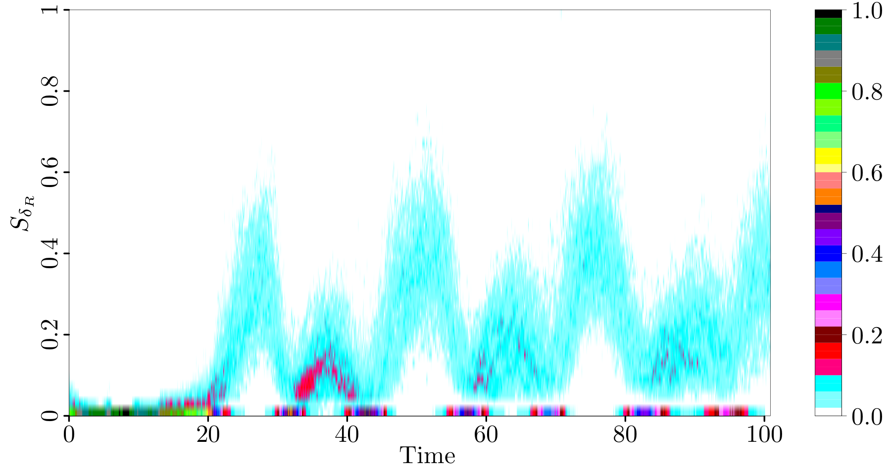
Our goal is to evaluate the sensitivity of the number of $\mathrm{C}$ molecules to the uncertain reaction rates. Letting the probability spaces $(\Theta,\mathcal{E},\nu)$ and $(\Omega,\mathcal{F},\mu)$ carry the intrinsic and the parametric randomness of the system, respectively, we note that $\mathrm{C}:\Theta\times\Omega\times[0,T_{\text{final}}]\to\mathbb{R}$ is a stochastic process. Figure 7 illustrates the dynamics of $\mathrm{C}=\mathrm{C}(\vartheta,\omega,t)$ by displaying four typical realizations of the stochastic process when the uncertain parameters are fixed at their nominal values. The differing periods and small oscillations are a result of the inherent stochasticity of the system.

Fig. 7: Genetic oscillator: four realizations of the evolution of the complex

C

We use Algorithm 2, with $n=400$ , $m=200$ , and MARS as the surrogate model. By subsampling $\Theta$ from our existing data, we assess convergence in $n$ and determine that $n=400$ is an adequate sample size for this application. Moreover, thanks to Proposition 1, a relatively small $m$ is sufficient to ensure a small variance of the estimators of the Sobol’ indices.

Figure 8, left, shows the time evolution of the expectation of the Sobol’ indices; for each index, the expectation becomes periodic after an initial transient. Moreover, we observe that the reaction rates $\beta_{R}$ and $\alpha_{R}^{\prime}$ have the most notable contribution to the model variance during the transient regime. After the transient regime, the degradation rates for the proteins $\mathrm{A}$ and $\mathrm{R}$ , i.e., $\delta_{A}$ and $\delta_{R}$ , are the most important factors. Figure 8, top right, displays the time evolution of the expectation of the Sobol’ indices for these two reaction rates. We note in particular that $\delta_{A}$ and $\delta_{R}$ periodically swap role of the most dominant contributor to variance of $\mathrm{C}$ after the intial transient regime. The time-dependent behavior of the statistical distribution of sensitivity index for $\delta_{R}$ is illustrated in Figure 8, bottom right.

The computational cost of the above analysis is $n\times m=400\times 200=80,000$ SSA simulations. While this is still a significant number of function evaluations, it should be contrasted with the complexity of traditional sampling based method for computing the Sobol’ indices, given in (12), which, for such a stochastic model, would be orders of magnitudes larger.

5 Summary and future work

We have proposed and investigated a strategy for the global sensitivity analysis of stochastic models. Within this framework, a thorough analysis of variable importance is obtained by computing the statistical properties of the Sobol’ indices. The proposed approach requires sampling in the product of probability spaces carrying the model stochasticity and parametric uncertainty. The number of samples in the uncertain parameter space is driven by the choice of surrogate model construction, and can be controlled via the use of adaptive surrogates such as MARS. We provide theoretical and numerical evidence that the moments of the indices can be evaluated with only a modest number of samples in the stochastic space.

As mentioned in the introduction, one may also consider performing sensitivity analysis on $\mathbb{E}_{\omega}\{f({\mathchoice{\mbox{\boldmath$\displaystyle{X}$}}{\mbox{\boldmath$\textstyle{X}$}}{\mbox{\boldmath$\scriptstyle{X}$}}{\mbox{\boldmath$\scriptscriptstyle{X}$}}},\omega)\}$ directly. However, as illustrated in Example 1.1, this approach may result in a significant loss of information. The variance of the Monte Carlo estimator for $E_{\omega}\{f({\mathchoice{\mbox{\boldmath$\displaystyle{X}$}}{\mbox{\boldmath$\textstyle{X}$}}{\mbox{\boldmath$\scriptstyle{X}$}}{\mbox{\boldmath$\scriptscriptstyle{X}$}}},\omega)\}$ is $\operatorname{Var}_{\omega}\{f({\mathchoice{\mbox{\boldmath$\displaystyle{X}$}}{\mbox{\boldmath$\textstyle{X}$}}{\mbox{\boldmath$\scriptstyle{X}$}}{\mbox{\boldmath$\scriptscriptstyle{X}$}}},\omega)\}/m$ , which in general is not known a priori. In contrast, the variance of the Monte Carlo estimator for $\mathbb{E}_{\omega}\{S_{u}(\omega)\}$ in our proposed framework is bounded above by $1/(4m)$ independently of $f$ . This gives our proposed method theoretical and computational advantages.

Our numerical results focus on computing first order Sobol’ indices and MARS was shown to be an efficient surrogate for this task. Higher order indices may be computed in our proposed framework as well, provided a sufficiently accurate surrogate model is available.

In our future work, we aim to address the following:

•

Thorough analysis of the role played by the surrogates both in terms of acting as possible screening mechanisms (as is the case for MARS) and regarding index approximation errors.
•

Explore the use of other surrogates to compute higher order indices in our framework.
•

Convergence analysis of the distributions of the Sobol’ indices and study of what can be inferred from them in light of surrogate induced biases.

References

[1] A. Alexanderian, J. Winokur, I. Sraj, A. Srinivasan, M. Iskandarani, W. C. Thacker, and O. M. Knio, Global sensitivity analysis in an ocean general circulation model: a sparse spectral projection approach, Computational Geosciences, 16 (2012), pp. 757–778.
[2] G. Arampatzis, M. Katsoulakis, and Y. Pantazis, Accelerated sensitivity analysis in high-dimensional stochastic reaction networks, PLOS ONE, 10 (2015), pp. e0130825–1–e0130825–24.
[3] R. Bhatia and C. Davis, A better bound on the variance, Mathematical Association of America, 107 (2000), pp. 353–357.
[4] G. Blatman and B. Sudret, Efficient computation of global sensitivity indices using sparse polynomial chaos expansions, Reliability Engineering & System Safety, 95 (2010), pp. 1216–1229.
[5] , Adaptive sparse polynomial chaos expansion based on least angle regression, Journal of Computational Physics, 230 (2011), pp. 2345–2367.
[6] P. R. Conrad and Y. M. Marzouk, Adaptive smolyak pseudospectral approximations, SIAM Journal on Scientific Computing, 35 (2013), pp. A2643–A2670.
[7] T. Crestaux, O. L. Maitre, and J.-M. Martinez, Polynomial chaos expansion for sensitivity analysis, Reliability Engineering & System Safety, 94 (2009), pp. 1161 – 1172. Special Issue on Sensitivity Analysis.
[8] A. Degasperi and S. Gilmore, Sensitivity analysis of stochastic models of bistable biochemical reactions, in Formal Methods for Computational Systems Biology, Springer, 2008, pp. 1–20.
[9] A. Doostan and H. Owhadi, A non-adapted sparse approximation of pdes with stochastic inputs, Journal of Computational Physics, 230 (2011), pp. 3015–3034.
[10] R. Durrett, Probability: Theory and Examples, Cambridge University Press, 4 ed., 2010.
[11] H. El Samad, M. Khammash, L. Petzold, and D. Gillespie, Stochastic modelling of gene regulatory networks, International Journal of Robust and Nonlinear Control, 15 (2005), pp. 691–711.
[12] J. Friedman, Multivariate adaptive regression splines, Ann. Stat., 19 (1991), pp. 1–67.
[13] , Fast MARS, Tech. Rep. 110, Laboratory for Computational Statistics, Department of Statistics, Stanford University, 1993.
[14] R. Ghanem and P. Spanos, Stochastic Finite Elements: A Spectral Approach, Dover, 2002. 2nd edition.
[15] D. Gillespie, A general method for numerically simulating the stochastic time evolution of coupled chemical reactions, J. Comput. Phys., 22 (1976), pp. 403–434.
[16] , Exact stochastic simulation of coupled chemical reactions, J. Phys. Chem., 81 (1977), pp. 2340–2361.
[17] R. Gunawan, Y. Cao, L. Petzold, and F. Doyle III, Sensitivity analysis of discrete stochastic systems, Biophys. J., 88 (2005), pp. 2530–2540.
[18] T. Hastie, R. Tibshirani, and J. Friedman, The elements of statistical learning, Springer Series in Statistics, Springer, New York, second ed., 2009. Data mining, inference, and prediction.
[19] B. Iooss and P. Le Maître, A review on global analysis methods, in Uncertainty management in simulation-optimization of complex systems, G. Dellino and C. Meloni, eds., Springer, 2015, ch. 5, pp. 501–543.
[20] B. Iooss and M. Ribatet, Global sensitivity analysis of computer models with functional inputs, Reliability Engineering & System Safety, 94 (2009), pp. 1194–1204.
[21] J. D. Jakeman, M. S. Eldred, and K. Sargsyan, Enhancing $\ell$ 1-minimization estimates of polynomial chaos expansions using basis selection, Journal of Computational Physics, 289 (2015), pp. 18–34.
[22] A. Janon, M. Nodet, and C. Prieur, Uncertainties assessment in global sensitivity indices estimation from metamodels, Int. J. Uncert. Quant., 4 (2014), pp. 21–36.
[23] D. Kim, B. Debusschere, and H. Najm, Spectral methods for parametric sensitivity in stochastic dynamical systems, Biophys. J., 92 (2007), pp. 379–393.
[24] J. Kleijnen and W. van Beers, Kriging for interpolation in random simulations, J. Oper. Res. Soc., 54 (2003), pp. 255–262.
[25] M. Komorowski, M. Costa, D. Rand, and M. Stumpf, Sensitivity, robustness, and identifiability in stochastic kinetics models, Proc. Natl. Acad. Sci. USA, 108 (2011), pp. 8645–8650.
[26] L. Le Gratiet, C. Cannamela, and B. Iooss, A Bayesian approach for global sensitivity analysis of (multifidelity) computer codes, SIAM/ASA J. Uncert. Quant., 2 (2014), pp. 336–363.
[27] L. Le Gratiet, S. Marelli, and B. Sudret, Metamodel-based sensitivity analysis: Polynomial chaos expansions and gaussian processes, in Handbook on Uncertainty Quantification, R. Ghanem, D. Higdon, and H. Owhadi, eds., Springer, 2016.
[28] O. Le Maître and O. Knio, Spectral Methods for Uncertainty Quantification With Applications to Computational Fluid Dynamics, Scientific Computation, Springer, 2010.
[29] O. Le Maître and O. Knio, PC analysis of stochastic differential equations driven by Wiener noise, Reliability Engineering & System Safety, 135 (2015), pp. 107–124.
[30] A. Majda and B. Gershgorin, Quantifying uncertainty in climate change science through empirical information theory, Proc. Natl. Acad. Sci. USA, 107 (2010), pp. 14958–14963.
[31] , Improving model fidelity and sensitivity for complex systems through empirical information theory, Proc. Natl. Acad. Sci. USA, 108 (2011), pp. 10044–10049.
[32] A. Marrel, Mise en oeuvre et exploitation du métamodèle processus gaussien pour l’analyse de modèles numériques - Application à un code de transport hydrogéologique, PhD thesis, INSA Toulouse, 2008.
[33] A. Marrel, B. Iooss, S. Da Veiga, and M. Ribatet, Global sensitivity analysis of stochastic computer models with joint metamodels, Stat. Comput., 22 (2012), pp. 833–847.
[34] S. Milborrow, Notes on the earth package, 2015. http://www.milbo.org/doc/earth-notes.pdf.
[35] M. Nakayama, A. Goyal, and P. Glynn, Likelihood ratio sensitivity analysis for markovian models of highly dependable systems, Stoch. Models, 10 (1994), pp. 701–717.
[36] O.P. Le Maître, O. Knio, and A. Moraes, Variance decomposition in stochastic simulators, J. Chem. Phys., 142 (2015), pp. 244115–1–244115–13.
[37] A. Owen, Better estimation of small Sobol’ indices sensitivity indices, ACM Trans. Mod. Comput. Simul., 23 (2013), pp. 11–1:11–17.
[38] S. Plyasunov and A. Arkin, Efficient stochastic sensitivity analysis of discrete event systems, J. Comput. Phys., 221 (2007), pp. 724–738.
[39] M. Rathinam, P. Sheppard, and M. Khammash, Efficient computation of parameter sensitivities of discrete stochastic chemical reaction networks, J. Chem. Phys, 132 (2010), pp. 034103–1–034103–13.
[40] J. Sacks, W. Welch, T. Mitchell, and H. Wynn, Design and analysis of computer experiments, Stat. Sci., 4 (1989), pp. 409–435.
[41] A. Saltelli, Making best use of model evaluations making best use of model evaluations to compute sensitivity indices, Computer Physics Communications, 145 (2002), pp. 280–297.
[42] A. Saltelli, M. Ratto, T. Andres, F. Campolongo, J. Cariboni, D. Gatelli, M. Saisana, and S. Tarantola, Global sensitivity analysis: the primer, Wiley, 2008.
[43] I. Sobol’, Sensitivity estimates for non linear mathematical models, Math. Mod. Comp. Exp., 1 (1993), pp. 407–414.
[44] I. Sobol’, Global sensitivity indices for nonlinear mathematical models and their Monte Carlo estimates, Mathematics and Computers in Simulation, 55 (2001), pp. 271–280.
[45] C. Storlie, L. Swiler, J. Helton, and C. Sallaberry, Implementation and evaluation of nonparametric regression procedures for sensitivity analysis of computationally demanding models, Reliability Eng. Sys. Safety, 94 (2009), pp. 1735–1763.
[46] B. Sudret, Global sensitivity analysis using polynomial chaos expansions, Reliability Engineering & System Safety, 93 (2008), pp. 964 – 979.
[47] E. van den Berg and M. P. Friedlander, SPGL1: A solver for large-scale sparse reconstruction, June 2007. http://www.cs.ubc.ca/labs/scl/spgl1.
[48] J. M. Vilar, H. Y. Kueh, N. Barkai, and S. Leibler, Mechanisms of noise-resistance in genetic oscillators, Proceedings of the National Academy of Sciences, 99 (2002), pp. 5988–5992.
[49] D. Wilkinson, Stochastic modelling for quantitative description of heterogeneous biological systems, Nature, 10 (2009), pp. 122–133.
[50] J. Winokur, D. Kim, F. Bisetti, O. Le Maître, and O. Knio, Sparse pseudo spectral projection methods with directional adaptation for uncertainty quantification, Journal of Scientific Computing, (2014), pp. 1–28.
[51] D. Xiu, Numerical methods for stochastic computations: a spectral method approach, Princeton University Press, 2010.