跳到论文正文
W Papers独立论文阅读器 arXiv:1602.06180 论文正文 计算阅读时间 · 0%
引用这篇论文根据当前论文元数据生成,正式投稿前建议核对。


License: arXiv.org perpetual non-exclusive license
arXiv:1602.06180v3 [math.OC] 05 Jun 2018

An Approach to Constrained Polynomial Optimization via Nonnegative Circuit Polynomials and Geometric Programming

Mareike Dressler Address: Mareike Dressler, Goethe-Universität, FB 12 – Institut für Mathematik, Postfach 11 19 32, 60054 Frankfurt am Main, Germany Email address: dressler@math.uni-frankfurt.de , Sadik Iliman Address: Sadik Iliman Frankfurt am Main, Germany Email address: sadik.iliman@gmx.net and Timo de Wolff Address: Timo de Wolff, Technische Universität Berlin, Institut für Mathematik, Straße des 17. Juni 136, 10623 Berlin, Germany Email address: dewolff@math.tu-berlin.de
Abstract.

In this article we combine two developments in polynomial optimization. On the one hand, we consider nonnegativity certificates based on sums of nonnegative circuit polynomials, which were recently introduced by the second and the third author. On the other hand, we investigate geometric programming methods for constrained polynomial optimization problems, which were recently developed by Ghasemi and Marshall. We show that the combination of both results yields a new method to solve certain classes of constrained polynomial optimization problems. We test the new method experimentally and compare it to semidefinite programming in various examples.

Key words and phrases: 
Certificate, geometric programming, nonnegative polynomial, semidefinite programming, sum of nonnegative circuit polynomials, sum of squares, triangulation
2010 Mathematics Subject Classification
12D15, 14P99, 52B20, 90C25

1. Introduction

Solving polynomial optimization problems is a key challenge in countless applications like dynamical systems, robotics, control theory, computer vision, signal processing, and economics; e.g. [BPT13, Las10]. It is well-known that polynomial optimization problems are NP-hard in general both in the constrained and in the unconstrained case [DG14]. Starting with the seminal work of Lasserre in [Las01], relaxation methods were developed which are significantly faster and provide lower bounds. These methods were studied intensively by means of aspects like exactness and quality of the relaxations [dKL10, Nie13a, Nie13b, Nie14], the speed of the computations [Las10, PS03], and geometrical aspects of the underlying structures [Ble06, Ble12]. A great majority of these results are based on the original approach by Lasserre, called Lasserre relaxation, which relies on semidefinite programming (SDP) methods and sums of squares (SOS) certificates to provide lower bounds for polynomial optimization problems. SDPs can be solved in polynomial time in problem size (up to an ε\varepsilon-error); e.g. [BPT13, p. 41] and references therein. However, the size of such programs grows exponentially with the number of variables nn or the degree dd of the polynomials, as its size is given by the number of monomials of nn-variate monomials of degree at most dd.

Recently, Ghasemi and Marshall suggested a promising alternative approach both for constrained and unconstrained optimization problems based on geometric programming (GP) [GM12, GM13]. GPs can also be solved in polynomial time (up to an ε\varepsilon-error) [NN94]; see also [BKVH07, Page 118], but, by experimental results, e.g. [BKVH07, GM12, GM13, GLM14], in practice the corresponding geometric programs can be solved significantly faster than their counterparts in semidefinite programming. The lower bounds obtained by Ghasemi and Marshall are, however, by construction worse than lower bounds obtained via semidefinite programming, and they can only be applied in very special cases.

Independent of Ghasemi and Marshall, the second and the third author recently developed a new certificate for nonnegativity of real polynomials called sums of nonnegative circuit polynomials (SONC) [IdW16a]. SONC certificates are independent of SOS certificates. In [IdW16b] the second and third author showed that the GP based approach for unconstrained optimization by Ghasemi and Marshall can be generalized crucially via SONC certificates. In consequence, the presented geometric programs are linked to sums of nonnegative circuit polynomials similarly as semidefinite programming relaxations are linked to sums of squares. Particularly, there exist various classes of polynomials for which the GP/SONC based approach is not only faster but, it also yields better bounds than the SDP/SOS approach. The reason is that all certificates used by Ghasemi and Marshall are always SOS, while SONCs are not SOS in general; see [IdW16a, Proposition 7.2].

The first contribution of this article is an extension of the results in [IdW16b] to constrained polynomial optimization problems. We focus on the class of ST-polynomials, that are polynomials which have a Newton polytope that is a simplex and which are satisfying some further conditions; see Section 2.1. The starting point is a general optimization problem from [IdW16b, Section 5], see (2.6), which provides a lower bound for the constrained problem but which is not a geometric program. Using results from [GM13], we relax the program (2.6) into a geometric optimization problem; see program (3.2) and Theorem 3.1. Additionally, we show in Theorem 3.4 that (2.6) can always at least be transformed into a signomial program; see Section 2.2 for background information. Furthermore, we prove that the new, relaxed geometric program (3.2) provides bounds as good as the initial program (2.6) for certain special cases, see Theorem 3.5.

In Section 4, we provide examples testing our new program (3.2) in practice and comparing it with semidefinite programming. Moreover, we demonstrate that increasing the degree of a given problem has almost no effect on the runtime of our program (3.2). This is in sharp contrast to SDPs, where one can nullify increased runtimes induced by high degrees only by additional pre-processing methods, e.g. by exploiting sparsity.

Furthermore, a bound obtained by Ghasemi and Marshall in [GM13] can never be better than the bound given by the dd-th Lasserre relaxation for some specific dd determined by the degrees of the involved polynomials. In Section 4 we provide examples showing that our program (3.2) can provide bounds which are better than the particularly dd-th Lasserre relaxations.

The second contribution of this article is to apply polynomial optimization methods based on SONCs and GPs efficiently beyond the class of ST-polynomials. In Section 5, we develop an initial approach based on triangulations of support sets of the involved polynomials. It yields bounds for nonnegativity based on SONC/GP for arbitrary polynomials both in the constrained and in the unconstrained case. We provide several examples and compare the new bounds to the ones obtained by SDP based methods.

Acknowledgements

We thank Henning Seidler for various comments and his support on some of the computations. We also thank the anonymous referees, who helped us to improve the article significantly.

The third author was partially supported by the DFG grant WO 2206/1-1.

2. Preliminaries

In this section we recall key results about sums of nonnegative circuit polynomials (SONCs) and geometric programming (GP), which are used in this article.

2.1. The Cone of Sums of Nonnegative Circuit Polynomials

We denote by ℝ⁡[𝐱]=ℝ⁡[x1,…,xn]\mathbb{R}[\mathbf{x}]=\mathbb{R}[x_{1},\ldots,x_{n}] the vector space of real nn-variate polynomials. Let δi​j\delta_{ij} be the i​jij-Kronecker symbol, let 𝐞i=(δi​1,…,δi​n){\color[rgb]{0.2,0.2,0.75}\mathbf{e}_{i}}=(\delta_{i1},\ldots,\delta_{in}) be the ii-th standard vector, and let A⊂ℕn{\color[rgb]{0.2,0.2,0.75}A}\subset\mathbb{N}^{n} be a finite set. We denote by conv⁡(A)\conv(A) the convex hull of AA and by V⁡(A)V(A) the vertices of conv⁡(A)\conv(A). We consider polynomials f∈ℝ⁡[𝐱]f\in\mathbb{R}[\mathbf{x}] supported on AA. That is, ff is of the form f⁡(𝐱)=∑𝜶∈Af𝜶​𝐱𝜶{\color[rgb]{0.2,0.2,0.75}f(\mathbf{x})}=\sum_{\boldsymbol{\alpha}\in A}f_{\boldsymbol{\alpha}}\mathbf{x}^{\boldsymbol{\alpha}} with f𝜶∈ℝ{\color[rgb]{0.2,0.2,0.75}f_{\boldsymbol{\alpha}}}\in\mathbb{R}, 𝐱𝜶=x1α1⋯xnαn{\color[rgb]{0.2,0.2,0.75}\mathbf{x}^{\boldsymbol{\alpha}}}=x_{1}^{\alpha_{1}}\cdots x_{n}^{\alpha_{n}}. We call a lattice point even if it is in (2​ℕ)n(2\mathbb{N})^{n}. Furthermore, we denote the Newton polytope of ff as New⁡(f)=conv⁡{𝜶∈ℕn:f𝜶≠0}{\color[rgb]{0.2,0.2,0.75}\New(f)}=\conv\{\boldsymbol{\alpha}\in\mathbb{N}^{n}:f_{\boldsymbol{\alpha}}\neq 0\}.

For a given A⊂ℕnA\subset\mathbb{N}^{n} we define Δ⁡(A)=A∖V⁡(A){\color[rgb]{0.2,0.2,0.75}\Delta(A)}=A\setminus V(A). Let ff be as before. We denote by Δ⁡(f)\Delta(f) the elements of Δ⁡(A)\Delta(A) which appear as exponents of non-zero terms, that are no monomial squares. I.e., we have

Δ⁡(f)\displaystyle{\color[rgb]{0.2,0.2,0.75}\Delta(f)} =\displaystyle= {𝜶∈Δ⁡(A):f𝜶≠0​ and ​(f𝜶<0​ or ​𝜶∉(2​ℕ)n)}.\displaystyle\{\boldsymbol{\alpha}\in\Delta(A)\ :\ f_{\boldsymbol{\alpha}}\neq 0\text{ and }(f_{\boldsymbol{\alpha}}<0\text{ or }\boldsymbol{\alpha}\notin(2\mathbb{N})^{n})\}.

A polynomial is nonnegative on the entire ℝn\mathbb{R}^{n} only if the following necessary conditions are satisfied; see e.g. [Rez78].

Proposition 2.1.

Let A⊂ℕnA\subset\mathbb{N}^{n} be a finite set and f∈ℝ⁡[𝐱]f\in\mathbb{R}[\mathbf{x}] be supported on AA such that New⁡(f)=conv⁡(A)\New(f)=\conv(A). Then ff is nonnegative on ℝn\mathbb{R}^{n} only if:

  1. (1)

    All elements of V⁡(A)V(A) are even.

  2. (2)

    If 𝜶∈V⁡(A)\boldsymbol{\alpha}\in V(A), then the corresponding coefficient f𝜶f_{\boldsymbol{\alpha}} is strictly positive.

In other words, if 𝛂∈V⁡(A)\boldsymbol{\alpha}\in V(A), then the term f𝛂​𝐱𝛂f_{\boldsymbol{\alpha}}\mathbf{x}^{\boldsymbol{\alpha}} has to be a monomial square.

The statement remains true for real Laurent polynomials g∈ℝ⁡[𝐱±1]=ℝ⁡[x1±1,…,xn±1]g\in\mathbb{R}[\mathbf{x}^{\pm 1}]=\mathbb{R}[x_{1}^{\pm 1},\ldots,x_{n}^{\pm 1}], since we can consider gg as a polynomial ff divided by a monomial square 𝐱𝜶\mathbf{x}^{\boldsymbol{\alpha}} for an even 𝜶\boldsymbol{\alpha}; this is of relevance in Section 5. For the remainder of the article, we assume that these necessary conditions in Proposition 2.1 are satisfied including New⁡(f)=conv⁡(A)\New(f)=\conv(A). For simplicity, we denote this assumption by the symbol (♣)(\clubsuit) from now on.

In what follows we consider the class of ST-polynomials. For further details about the following objects defined in this section see [dW15, IdW16a, IdW16b]; see also [FK11, GM12, GM13].

Definition 2.2.

Let f∈ℝ⁡[𝐱]f\in\mathbb{R}[\mathbf{x}] be supported on A⊂ℕnA\subset\mathbb{N}^{n} such that (♣)(\clubsuit) holds. Then ff is called an ST-polynomial if it is of the form

(2.1) f⁡(𝐱)\displaystyle{\color[rgb]{0.2,0.2,0.75}f(\mathbf{x})} =\displaystyle= ∑j=0rf𝜶⁡(j)​𝐱𝜶⁡(j)+∑𝜷∈Δ⁡(A)f𝜷​𝐱𝜷,\displaystyle\sum_{j=0}^{r}f_{\boldsymbol{\alpha}(j)}\mathbf{x}^{\boldsymbol{\alpha}(j)}+\sum_{\boldsymbol{\beta}\in\Delta(A)}f_{\boldsymbol{\beta}}\mathbf{x}^{\boldsymbol{\beta}},

with r≤n{\color[rgb]{0.2,0.2,0.75}r}\leq n, exponents 𝜶⁡(j){\color[rgb]{0.2,0.2,0.75}\boldsymbol{\alpha}(j)} and 𝜷{\color[rgb]{0.2,0.2,0.75}\boldsymbol{\beta}}, and coefficients f𝜶⁡(j),f𝜷{\color[rgb]{0.2,0.2,0.75}f_{\boldsymbol{\alpha}(j)}},{\color[rgb]{0.2,0.2,0.75}f_{\boldsymbol{\beta}}}, for which the following conditions hold:

(ST1):

The points 𝜶⁡(0),𝜶⁡(1),…,𝜶⁡(r)\boldsymbol{\alpha}(0),\boldsymbol{\alpha}(1),\ldots,\boldsymbol{\alpha}(r) are affinely independent and equal V⁡(A)V(A).

(ST2):

Every exponent 𝜷∈Δ⁡(A)\boldsymbol{\beta}\in\Delta(A) can be written uniquely as

𝜷=∑j=0rλj(𝜷)​𝜶​(j)​ with ​λj(𝜷)≥ 0​ and ​∑j=0rλj(𝜷)= 1.\displaystyle\boldsymbol{\beta}\ =\ \sum_{j=0}^{r}\lambda_{j}^{(\boldsymbol{\beta})}\boldsymbol{\alpha}(j)\ \text{ with }\ \lambda_{j}^{(\boldsymbol{\beta})}\ \geq\ 0\ \text{ and }\ \sum_{j=0}^{r}\lambda_{j}^{(\boldsymbol{\beta})}\ =\ 1.

⎔\hexagon

Note that hypotheses (ST1) and (ST2) imply that V⁡(A)={𝜶⁡(0),…,𝜶⁡(r)}V(A)=\{\boldsymbol{\alpha}(0),\ldots,\boldsymbol{\alpha}(r)\} is the vertex set of an rr-dimensional simplex. By the assumption (♣)(\clubsuit) it consists of even lattice points, and it coincides with New⁡(f)=conv⁡(A)\New(f)=\conv(A). The λj(𝜷){\color[rgb]{0.2,0.2,0.75}\lambda_{j}^{(\boldsymbol{\beta})}} denote the barycentric coordinates of 𝜷\boldsymbol{\beta} relative to the vertices 𝜶⁡(j)\boldsymbol{\alpha}(j) with j=0,…,rj=0,\ldots,r. The “ST” in “ST-polynomial” is short for “simplex tail”. The tail part is given by the sum ∑𝜷∈Δ⁡(A)f𝜷​𝐱𝜷,\sum_{\boldsymbol{\beta}\in\Delta(A)}f_{\boldsymbol{\beta}}\mathbf{x}^{\boldsymbol{\beta}}, while the other terms define the simplex part. If an ST-polynomial ff has a tail part consisting of at most one term, then we call ff a circuit polynomial.

Nonnegativity of ST-polynomials is closely related to an invariant called the circuit number.

Definition 2.3.

Let ff be an ST-polynomial with support set AA. For every 𝜷∈Δ⁡(A)\boldsymbol{\beta}\in\Delta(A) we define the corresponding circuit number as

(2.2) Θf​(𝜷)=∏j∈nz⁡(𝜷)(f𝜶⁡(j)λj(𝜷))λj(𝜷)\displaystyle{\color[rgb]{0.2,0.2,0.75}\Theta_{f}(\boldsymbol{\beta})}\ =\ \prod_{j\in{\rm nz}(\boldsymbol{\beta})}\left(\frac{f_{\boldsymbol{\alpha}(j)}}{\lambda_{j}^{(\boldsymbol{\beta})}}\right)^{\lambda_{j}^{(\boldsymbol{\beta})}}

with nz⁡(𝜷)={j∈{0,…,r}:λj(𝜷)≠0}{\color[rgb]{0.2,0.2,0.75}{\rm nz}(\boldsymbol{\beta})}=\{j\in\{0,\ldots,r\}:\lambda_{j}^{(\boldsymbol{\beta})}\neq 0\}, f𝜶⁡(j)f_{\boldsymbol{\alpha}(j)}, and λj(𝜷)\lambda_{j}^{(\boldsymbol{\beta})} as before. ⎔\hexagon

The terms “circuit polynomial” and “circuit number” are chosen since 𝜷\boldsymbol{\beta} and the 𝜶⁡(j)\boldsymbol{\alpha}(j) with j∈nz⁡(𝜷)j\in{\rm nz}(\boldsymbol{\beta}) form a circuit; this is a minimally affine dependent set, see e.g. [Oxl11].

A fundamental fact is that nonnegativity of a circuit polynomial ff can be decided by comparing its tail coefficient f𝜷f_{\boldsymbol{\beta}} with its corresponding circuit number Θf​(𝜷)\Theta_{f}(\boldsymbol{\beta}) alone.

Theorem 2.4 ([IdW16a], Theorem 3.8).

Let ff be a circuit polynomial with unique tail term f𝛃​𝐱𝛃f_{\boldsymbol{\beta}}\mathbf{x}^{\boldsymbol{\beta}} and let Θf​(𝛃)\Theta_{f}(\boldsymbol{\beta}) be the corresponding circuit number, as defined in (2.2). Then the following statements are equivalent:

  1. (1)

    ff is nonnegative.

  2. (2)

    |f𝜷|≤Θf​(𝜷)|f_{\boldsymbol{\beta}}|\leq\Theta_{f}(\boldsymbol{\beta}) and 𝜷∉(2​ℕ)n\boldsymbol{\beta}\not\in(2\mathbb{N})^{n}  or  f𝜷≥−Θf​(𝜷)f_{\boldsymbol{\beta}}\geq-\Theta_{f}(\boldsymbol{\beta}) and 𝜷∈(2​ℕ)n\boldsymbol{\beta}\in(2\mathbb{N})^{n}.

Note that (2) can be equivalently stated as: |f𝜷|≤Θf​(𝜷)|f_{\boldsymbol{\beta}}|\leq\Theta_{f}(\boldsymbol{\beta}) or ff is a sum of monomial squares.

Writing a polynomial as a sum of nonnegative circuit polynomials is a certificate of nonnegativity. We denote by SONC the class of polynomials that are sums of nonnegative circuit polynomials or the property of a polynomial to be in this class.

2.2. Geometric Programming

Geometric programming was introduced in [DPZ67]. It is a convex optimization problem and has applications for example in nonlinear network flow problems, optimal control, optimal location problems, chemical equilibrium problems and particularly in circuit design problems.

Definition 2.5.

A function p:ℝ>0n→ℝp:\mathbb{R}_{>0}^{n}\to\mathbb{R} of the form p(𝐳)=p(z1,…,zn)=cz1α1⋯znαn{\color[rgb]{0.2,0.2,0.75}p(\mathbf{z})}=p(z_{1},\ldots,z_{n})=cz_{1}^{\alpha_{1}}\cdots z_{n}^{\alpha_{n}} with c>0c>0 and αi∈ℝ\alpha_{i}\in\mathbb{R} is called a monomial (function). A sum ∑i=0kciz1α1​(i)⋯znαn​(i){\color[rgb]{0.2,0.2,0.75}\sum_{i=0}^{k}c_{i}z_{1}^{\alpha_{1}(i)}\cdots z_{n}^{\alpha_{n}(i)}} of monomials with ci>0c_{i}>0 is called a posynomial (function).

A geometric program (GP) has the following form:

(2.3) {minimizep0​(𝐳),subject to:(1)pi​(𝐳)≤1​ for all ​ 1≤i≤m,(2)qj​(𝐳)=1​ for all ​ 1≤j≤l,\displaystyle\begin{cases}\text{minimize}&p_{0}(\mathbf{z}),\\ \text{subject to:}&\begin{array}[]{cl}(1)&p_{i}(\mathbf{z})\leq 1\ \text{ for all }\ 1\leq i\leq m,\\ (2)&q_{j}(\mathbf{z})=1\ \text{ for all }\ 1\leq j\leq l,\\ \end{array}\end{cases}

where p0,…,pmp_{0},\dots,p_{m} are posynomials and q1,…,qlq_{1},\dots,q_{l} are monomial functions. ⎔\hexagon

Geometric programs can be solved with interior point methods. In [NN94], the authors prove worst-case polynomial time complexity of this method; see also [BKVH07, Page 118]. A signomial program is given like a geometric program except that the coefficients cic_{i} of the involved posynomials can be arbitrary real numbers.

For an introduction to geometric programming, signomial programming, and an overview about applications see [BKVH07, BV04].

2.3. SONC Certificates via Geometric Programming in the Unconstrained Case

In this section we recall the main results from [IdW16b] about SONC certificates obtained via geometric programming for unconstrained polynomial optimization problems. These results always require that the polynomial in the optimization problem is an ST-polynomial in the sense of Section 2.1.

Theorem 2.6.

([IdW16b, Theorems 3.4 and 3.5]) Assume that ff is an ST-polynomial as in (2.1) with 𝛂⁡(0)=0\boldsymbol{\alpha}(0)=0 and let k∈ℝ.k\in\mathbb{R}. Suppose that for every (𝛃,j)∈Δ⁡(f)×{1,…,r}(\boldsymbol{\beta},j)\in\Delta(f)\times\{1,\ldots,r\} there exists an a𝛃,j≥0,a_{\boldsymbol{\beta},j}\geq 0, such that:

  1. (1)

    a𝜷,j>0a_{\boldsymbol{\beta},j}>0 if and only if λj(𝜷)>0\lambda_{j}^{(\boldsymbol{\beta})}>0,

  2. (2)

    |f𝜷|≤∏j∈nz⁡(𝜷)(a𝜷,jλj(𝜷))λj(𝜷)|f_{\boldsymbol{\beta}}|\leq\prod\limits_{j\in{\rm nz}(\boldsymbol{\beta})}\left(\frac{a_{\boldsymbol{\beta},j}}{\lambda_{j}^{(\boldsymbol{\beta})}}\right)^{\lambda_{j}^{(\boldsymbol{\beta})}}   for every 𝜷∈Δ⁡(f)\boldsymbol{\beta}\in\Delta(f) with λ0(𝜷)=0\lambda_{0}^{(\boldsymbol{\beta})}=0,

  3. (3)

    f𝜶⁡(j)≥∑𝜷∈Δ⁡(f)a𝜷,jf_{\boldsymbol{\alpha}(j)}\geq\sum\limits_{\boldsymbol{\beta}\in\Delta(f)}a_{\boldsymbol{\beta},j} for all 1≤j≤r,1\leq j\leq r,

  4. (4)

    f𝜶⁡(0)−k≥∑𝜷∈Δ⁡(f)λ0(𝜷)≠0λ0(𝜷)​|f𝜷|1/λ0(𝜷)​∏j∈nz⁡(𝜷)j≥1(λj(𝜷)a𝜷,j)λj(𝜷)/λ0(𝜷).f_{\boldsymbol{\alpha}(0)}-k\geq\sum\limits_{\begin{subarray}{c}\boldsymbol{\beta}\in\Delta(f)\\ \lambda_{0}^{(\boldsymbol{\beta})}\neq 0\end{subarray}}\lambda_{0}^{(\boldsymbol{\beta})}|f_{\boldsymbol{\beta}}|^{1/\lambda_{0}^{(\boldsymbol{\beta})}}\prod\limits_{\begin{subarray}{c}j\in{\rm nz}(\boldsymbol{\beta})\\ j\geq 1\end{subarray}}\left(\frac{\lambda_{j}^{(\boldsymbol{\beta})}}{a_{\boldsymbol{\beta},j}}\right)^{\lambda_{j}^{(\boldsymbol{\beta})}/\lambda_{0}^{(\boldsymbol{\beta})}}.

Then f−kf-k is a sum of nonnegative circuit polynomials g1,…,gsg_{1},\ldots,g_{s} such that s:=|Δ⁡(f)|s:=|\Delta(f)|, and for every gig_{i} the Newton polytope New⁡(gi)\New(g_{i}) is a face of New⁡(f)\New(f).

Let fsonc{\color[rgb]{0.2,0.2,0.75}f_{\rm sonc}} be the supremum of all k∈ℝk\in\mathbb{R} such that for every 𝛃∈Δ⁡(f)\boldsymbol{\beta}\in\Delta(f) there exist nonnegative reals a𝛃,1,…,a𝛃,ra_{\boldsymbol{\beta},1},\ldots,a_{\boldsymbol{\beta},r} such that the conditions (1)(1) to (4)(4) are satisfied. Then fsoncf_{\rm sonc} coincides with the supremum of all k∈ℝk\in\mathbb{R} such that there exist nonnegative circuit polynomials g1,g2,…,gsg_{1},g_{2},\ldots,g_{s} whose Newton polytopes are faces of New⁡(f)\New(f) and which satisfy f−k=∑i=1sgi.f-k=\sum_{i=1}^{s}g_{i}.

We remark that Theorem 2.6 remains valid if all terms of an ST-polynomial are multiplied by a monomial square 𝐱𝜶⁡(0)∈(2​ℕ)n\mathbf{x}^{\boldsymbol{\alpha}(0)}\in(2\mathbb{N})^{n}. In this case, condition needs to be replaced by

  1. (4′)(4^{\prime})

    (f𝜶⁡(0)−k)​𝐱𝜶⁡(0)≥∑𝜷∈Δ⁡(f)λ0(𝜷)≠0λ0(𝜷)​|f𝜷|1/λ0(𝜷)​∏j∈nz⁡(𝜷)j≥1(λj(𝜷)a𝜷,j)λj(𝜷)/λ0(𝜷).(f_{\boldsymbol{\alpha}(0)}-k)\mathbf{x}^{\boldsymbol{\alpha}(0)}\geq\sum\limits_{\begin{subarray}{c}\boldsymbol{\beta}\in\Delta(f)\\ \lambda_{0}^{(\boldsymbol{\beta})}\neq 0\end{subarray}}\lambda_{0}^{(\boldsymbol{\beta})}|f_{\boldsymbol{\beta}}|^{1/\lambda_{0}^{(\boldsymbol{\beta})}}\prod\limits_{\begin{subarray}{c}j\in{\rm nz}(\boldsymbol{\beta})\\ j\geq 1\end{subarray}}\left(\frac{\lambda_{j}^{(\boldsymbol{\beta})}}{a_{\boldsymbol{\beta},j}}\right)^{\lambda_{j}^{(\boldsymbol{\beta})}/\lambda_{0}^{(\boldsymbol{\beta})}}.

We then obtain a nonnegativity bound for the (positive) the coefficient of the term 𝐱𝜶⁡(0)\mathbf{x}^{\boldsymbol{\alpha}(0)} instead of the constant term. We apply this slightly more general version of Theorem 2.6 in Section 5.

For the special case of scaled standard simplices Theorem 2.6 was shown earlier by Ghasemi and Marshall [GM12, Theorem 3.1]. In this special case every sum of nonnegative circuit polynomials is also a sum of binomial squares which is not true in general. For example, the Motzkin polynomial is an ST-polynomial with one interior term, which is not even a SOS.

Theorem 2.6 states

fsonc\displaystyle f_{\rm sonc} =\displaystyle= sup{k∈ℝ:f−k​𝐱𝜶⁡(0)​ is a SONC}.\displaystyle\sup\{k\in\mathbb{R}\ :\ f-k\mathbf{x}^{\boldsymbol{\alpha}(0)}\text{ is a SONC}\,\}.

The bound fsoncf_{\rm sonc} is given by a geometric program [IdW16b, Corollary 4.2]:

Corollary 2.7.

Let f∈ℝ⁡[𝐱]f\in\mathbb{R}[\mathbf{x}] be an ST-polynomial. Let RR be the subset of an r​|Δ⁡(f)|r|\Delta(f)|-dimensional real space given by

R\displaystyle{\color[rgb]{0.2,0.2,0.75}R} =\displaystyle= {(a𝜷,j):a𝜷,j∈ℝ>0​ for every ​𝜷∈Δ⁡(f)​ and ​j∈nz⁡(𝜷)}.\displaystyle\{(a_{\boldsymbol{\beta},j})\ :\ a_{\boldsymbol{\beta},j}\in\mathbb{R}_{>0}\text{ for every }\boldsymbol{\beta}\in\Delta(f)\text{ and }j\in{\rm nz}(\boldsymbol{\beta})\}.

Then fsonc=f𝛂⁡(0)−m∗,f_{\rm sonc}=f_{\boldsymbol{\alpha}(0)}-m^{*}, where m∗{\color[rgb]{0.2,0.2,0.75}m^{*}} is given as the output of the following geometric program:

{​m​i​n​i​m​i​z​e∑𝜷∈Δ⁡(f)λ0(𝜷)≠0λ0(𝜷)|f𝜷|∏j∈nz⁡(𝜷)j≥11/λ0(𝜷)⁡(λj(𝜷)a𝜷,j)λj(𝜷)/λ0(𝜷)​​o​v​e​r​t​h​e​s​u​b​s​e​t​R′​​o​f​R​d​e​f​i​n​e​d​b​y:(1)∑𝜷∈Δ⁡(f)(a𝜷,j/f𝜶⁡(j))≤1​​f​o​r​e​v​e​r​y​1≤j≤r,(2)|f𝜷|​∏j∈nz⁡(𝜷)(λj(𝜷)a𝜷,j)λj(𝜷)≤1​​f​o​r​e​v​e​r​y​𝜷∈Δ⁡(f)​​w​i​t​h​λ0(𝜷)=0.\displaystyle\begin{cases}\emph{minimize}&\sum\limits_{\begin{subarray}{c}\boldsymbol{\beta}\in\Delta(f)\\ \lambda_{0}^{(\boldsymbol{\beta})}\neq 0\end{subarray}}\lambda_{0}^{(\boldsymbol{\beta})}|f_{\boldsymbol{\beta}}|^{1/\lambda_{0}^{(\boldsymbol{\beta})}}\prod\limits_{\begin{subarray}{c}j\in{\rm nz}(\boldsymbol{\beta})\\ j\geq 1\end{subarray}}\left(\frac{\lambda_{j}^{(\boldsymbol{\beta})}}{a_{\boldsymbol{\beta},j}}\right)^{\lambda_{j}^{(\boldsymbol{\beta})}/\lambda_{0}^{(\boldsymbol{\beta})}}\emph{overthesubset}R^{\prime}\emph{of}R\\ &\\ \emph{definedby:}&\begin{array}[]{cl}(1)&\sum\limits_{\boldsymbol{\beta}\in\Delta(f)}(a_{\boldsymbol{\beta},j}/f_{\boldsymbol{\alpha}(j)})\leq 1\emph{forevery}1\leq j\leq r,\\ (2)&|f_{\boldsymbol{\beta}}|\prod\limits_{j\in{\rm nz(\boldsymbol{\beta})}}\left(\frac{\lambda_{j}^{(\boldsymbol{\beta})}}{a_{\boldsymbol{\beta},j}}\right)^{\lambda_{j}^{(\boldsymbol{\beta})}}\leq 1\emph{forevery}\boldsymbol{\beta}\in\Delta(f)\emph{with}\lambda_{0}^{(\boldsymbol{\beta})}=0.\\ \end{array}\end{cases}

Hence, the optimal bound to find a SONC decomposition of an ST-polynomial is provided by geometric programming. Since a polynomial with a SONC decomposition is nonnegative, geometric programming can be used to find certificates of nonnegativity.

Following the literature, e.g. [BPT13, Lau09], we define a global polynomial optimization problem for some f∈ℝ⁡[𝐱]f\in\mathbb{R}[\mathbf{x}] as the problem to determine the real number

f∗\displaystyle{\color[rgb]{0.2,0.2,0.75}f^{*}} =\displaystyle= inf{f⁡(𝐱):𝐱∈ℝn}=sup{λ∈ℝ:f−λ≥0}.\displaystyle\inf\{f(\mathbf{x})\ :\ \mathbf{x}\in\mathbb{R}^{n}\}\ =\ \sup\{\lambda\in\mathbb{R}\ :\ f-\lambda\geq 0\}.

One can find a lower bound for f∗f^{*} by relaxing the nonnegativity condition in the above problem to finding the real number

fsos\displaystyle{\color[rgb]{0.2,0.2,0.75}f_{\rm sos}} =\displaystyle= sup{λ∈ℝ:f−λ=∑i=1kqi2​ for some ​qi∈ℝ⁡[𝐱]}.\displaystyle\sup\left\{\lambda\in\mathbb{R}\ :\ f-\lambda=\sum_{i=1}^{k}q_{i}^{2}\ \text{ for some }\ q_{i}\in\mathbb{R}[\mathbf{x}]\right\}.

The bound fsosf_{\rm sos} for the optimal SOS decomposition of ff can be determined by semidefinite programming. By construction, we have fsos≤f∗f_{\rm sos}\leq f^{*}; see [Las10].

A key observation is that the bounds obtained by this approach can be better than the ones obtained by SDP as the following result shows; see [IdW16b, Corollary 3.6].

Corollary 2.8.

Let ff be an ST-polynomial with Δ⁡(A)=Δ⁡(f)\Delta(A)=\Delta(f) such that Δ⁡(f)\Delta(f) is contained in the interior of New⁡(f)\New(f). Let 𝛂⁡(0)\boldsymbol{\alpha}(0) be the origin and suppose that there exists a vector 𝐯∈(ℝ∗)n\mathbf{v}\in(\mathbb{R}^{*})^{n} such that f𝛂⋅𝐯𝛂<0f_{\boldsymbol{\alpha}}\cdot\mathbf{v}^{\boldsymbol{\alpha}}<0 for all 𝛂∈Δ⁡(f)\boldsymbol{\alpha}\in\Delta(f). Then

fsonc=f∗≥fsos.\displaystyle f_{\rm sonc}\ =\ f^{*}\ \geq\ f_{\rm sos}.

2.4. SONC Certificates for the Constrained Case

In this subsection we restate facts from [IdW16b, Section 5] about SONC certificates applied to constrained polynomial optimization problems.

Let f,g1,…,gsf,g_{1},\ldots,g_{s} be elements of the polynomial ring ℝ⁡[𝐱]\mathbb{R}[\mathbf{x}] and let

K={𝐱∈ℝn:gi(𝐱)≥0 for all i=1,…,s}\displaystyle{\color[rgb]{0.2,0.2,0.75}K}\ =\ \{\mathbf{x}\in\mathbb{R}^{n}\ :\ g_{i}(\mathbf{x})\geq 0\text{ for all }i=1,\ldots,s\}

be a basic closed semialgebraic set defined by g1,…,gsg_{1},\ldots,g_{s}. We consider the constrained polynomial optimization problem

fK∗=inf𝐱∈Kf⁡(𝐱)=sup{γ∈ℝ:f⁡(𝐱)−γ≥0​ for all ​𝐱∈K}.\displaystyle{\color[rgb]{0.2,0.2,0.75}f_{K}^{*}}\ =\ \inf_{\mathbf{x}\in K}f(\mathbf{x})\ =\ \sup\{\gamma\in\mathbb{R}\ :\ f(\mathbf{x})-\gamma\geq 0\;\text{ for all }\mathbf{x}\in K\}.

If s=0s=0, then we have no gig_{i} and therefore K=ℝnK=\mathbb{R}^{n}, which leads to the global optimization problem explained in Section 2.3.

To obtain a general lower bound for ff on KK which is computable by geometric programming we replace the considered polynomials by a new function. Let

(2.4) G(𝝁)(𝐱)=f(𝐱)−∑i=1sμigi(𝐱)=−∑i=0sμigi(𝐱)\displaystyle{\color[rgb]{0.2,0.2,0.75}G(\boldsymbol{\mu})(\mathbf{x})}\ =\ f(\mathbf{x})-\sum_{i=1}^{s}\mu_{i}g_{i}(\mathbf{x})\ =\ -\sum_{i=0}^{s}\mu_{i}g_{i}(\mathbf{x})

for 𝝁=(μ1,…,μs)∈ℝ≥0s{\color[rgb]{0.2,0.2,0.75}\boldsymbol{\mu}}=(\mu_{1},\dots,\mu_{s})\in\mathbb{R}_{\geq 0}^{s}, g0=−f{\color[rgb]{0.2,0.2,0.75}g_{0}}=-f and μ0=1{\color[rgb]{0.2,0.2,0.75}\mu_{0}}=1. For every fixed 𝝁∗∈ℝ≥0s\boldsymbol{\mu}^{*}\in\mathbb{R}_{\geq 0}^{s} the function G⁡(𝐱)=G⁡(𝝁∗)​(𝐱){\color[rgb]{0.2,0.2,0.75}G(\mathbf{x})}=G(\boldsymbol{\mu}^{*})(\mathbf{x}) is a polynomial in ℝ⁡[𝐱]\mathbb{R}[\mathbf{x}]. Following an argument in [GM13] we can assume that all monomial squares of −gi-g_{i} are vertices of New⁡(G⁡(𝝁))\New(G(\boldsymbol{\mu})): One can reduce to this case by neglecting all monomial squares not corresponding to such a vertex. That is, for all i=0,…,si=0,\ldots,s one can replace gig_{i} by g~i\tilde{g}_{i}, which resemble gig_{i} without monomial squares of −gi-g_{i} in the interior of New⁡(G⁡(𝝁))\New(G(\boldsymbol{\mu})). Then −g~i≤−gi-\tilde{g}_{i}\leq-g_{i} on ℝn\mathbb{R}^{n} for i=0,…,si=0,\ldots,s, thus, K⊆K~K\subseteq\tilde{K}, where K~={𝐱∈ℝn:g~i(𝐱)≥0,  1≤i≤s}\tilde{K}=\{\mathbf{x}\in\mathbb{R}^{n}\ :\ \tilde{g}_{i}(\mathbf{x})\geq 0,\,\,1\leq i\leq s\}, as well as fK~∗≤fK∗f_{\tilde{K}}^{*}\leq f_{K}^{*}.

Let Ai⊂ℕn{\color[rgb]{0.2,0.2,0.75}A_{i}}\subset\mathbb{N}^{n} be the support of the polynomial gig_{i} for i=0,…,si=0,\ldots,s and let A=⋃i=0sAi{\color[rgb]{0.2,0.2,0.75}A}=\bigcup_{i=0}^{s}A_{i} be the union of all supports of polynomials gig_{i}. We remark that while we consider a fixed support the Newton polytope of G⁡(𝝁)G(\boldsymbol{\mu}) is not invariant in general since certain μi\mu_{i} might equal 00 or term cancellation might occur. If for some 𝝁∈ℝ≥0s\boldsymbol{\mu}\in\mathbb{R}_{\geq 0}^{s} the polynomial G⁡(𝝁)G(\boldsymbol{\mu}) is an ST-polynomial, then we assume that New⁡(G⁡(𝝁))=conv⁡(A)\New(G(\boldsymbol{\mu}))=\conv(A) and V⁡(A)={𝜶⁡(0),…,𝜶⁡(r)}⊂(2​ℕ)nV(A)=\{\boldsymbol{\alpha}(0),\ldots,\boldsymbol{\alpha}(r)\}\subset(2\mathbb{N})^{n} and we denote G​(𝝁)sonc{\color[rgb]{0.2,0.2,0.75}G(\boldsymbol{\mu})_{\rm sonc}} as the optimal value of the geometric program in Corollary 2.7. Theorem 2.6 implies that G⁡(𝝁)−G​(𝝁)sonc​𝐱𝜶⁡(0)≥0G(\boldsymbol{\mu})-G(\boldsymbol{\mu})_{\rm sonc}\mathbf{x}^{\boldsymbol{\alpha}(0)}\geq 0 and G​(𝝁)sonc∈ℝG(\boldsymbol{\mu})_{\rm sonc}\in\mathbb{R} is the maximal possible choice for nonnegativity. Hence, we obtain a bound for the coefficient of the term 𝐱𝜶⁡(0)\mathbf{x}^{\boldsymbol{\alpha}(0)} depending on the other coefficients of G⁡(𝝁)G(\boldsymbol{\mu}) certifying nonnegativity of G⁡(𝝁)G(\boldsymbol{\mu}). If G⁡(𝝁)G(\boldsymbol{\mu}) is not an ST-polynomial for some 𝝁∈ℝ≥0s\boldsymbol{\mu}\in\mathbb{R}_{\geq 0}^{s}, then we set G​(𝝁)sonc=−∞G(\boldsymbol{\mu})_{\rm sonc}=-\infty, since the corresponding geometric program is infeasible. Thus, by (2.4), if 𝝁\boldsymbol{\mu} is fixed, then G​(𝝁)soncG(\boldsymbol{\mu})_{\rm sonc} is a lower bound for ff on the semialgebraic set KK regarding the coefficient of 𝐱𝜶⁡(0)\mathbf{x}^{\boldsymbol{\alpha}(0)}. Let 𝐠=(g1,…,gs){\color[rgb]{0.2,0.2,0.75}\mathbf{g}}=(g_{1},\dots,g_{s}). We define

s⁡(f,𝐠)=sup{G​(𝝁)sonc:𝝁∈ℝ≥0s}.\displaystyle{\color[rgb]{0.2,0.2,0.75}s(f,\mathbf{g})}\ =\ \sup\{G(\boldsymbol{\mu})_{\rm sonc}:\boldsymbol{\mu}\in\mathbb{R}_{\geq 0}^{s}\}.

Thus, we have particularly for 𝜶⁡(0)=𝟎\boldsymbol{\alpha}(0)=\mathbf{0}:

(2.5) s⁡(f,𝐠)≤fK∗.\displaystyle s(f,\mathbf{g})\ \leq\ f_{K}^{*}.

For every fixed 𝝁\boldsymbol{\mu} the bound G​(𝝁)soncG(\boldsymbol{\mu})_{\rm sonc} is computable by a geometric program. Unfortunately, this does not imply that the supremum is computable by a GP as well. However, following ideas by Ghasemi and Marshall [GM12] the second and third author presented a general optimization program for a lower bound of s⁡(f,𝐠)s(f,\mathbf{g}) in [IdW16b], which is a geometric program under special conditions. We recall these results in what follows.

We define Δ⁡(A){\color[rgb]{0.2,0.2,0.75}\Delta(A)} in the sense of Section 2.1 as the set of exponents of the tail terms of G⁡(𝝁)G(\boldsymbol{\mu}) and Δ⁡(G⁡(𝝁))⊆Δ⁡(A){\color[rgb]{0.2,0.2,0.75}\Delta(G(\boldsymbol{\mu}))}\subseteq\Delta(A) as the set of exponents which have a non-zero coefficient and are not a monomial square. Moreover, we define Δ⁡(G)=⋃𝝁∈ℝ≥0sΔ⁡(G⁡(𝝁)){\color[rgb]{0.2,0.2,0.75}\Delta(G)}=\bigcup_{\boldsymbol{\mu}\in\mathbb{R}^{s}_{\geq 0}}\Delta(G(\boldsymbol{\mu})). Note that Δ⁡(G⁡(𝝁))⊆Δ⁡(G)⊆Δ⁡(A)\Delta(G(\boldsymbol{\mu}))\subseteq\Delta(G)\subseteq\Delta(A) for all 𝝁\boldsymbol{\mu}. We have by Section 2.1, Definition 2.2

G(𝝁)(𝐱)=−∑i=0sμigi(𝐱)=∑j=0rG(𝝁)𝜶⁡(j)𝐱𝜶⁡(j)+∑𝜷∈Δ⁡(G)G(𝝁)𝜷𝐱𝜷\displaystyle G(\boldsymbol{\mu})(\mathbf{x})\ =\ -\sum_{i=0}^{s}\mu_{i}g_{i}(\mathbf{x})\ =\ \sum_{j=0}^{r}G(\boldsymbol{\mu})_{\boldsymbol{\alpha}(j)}\mathbf{x}^{\boldsymbol{\alpha}(j)}+\sum_{\boldsymbol{\beta}\in\Delta(G)}G(\boldsymbol{\mu})_{\boldsymbol{\beta}}\mathbf{x}^{\boldsymbol{\beta}}

with coefficients G​(𝝁)𝜶⁡(j),G​(𝝁)𝜷∈ℝ{\color[rgb]{0.2,0.2,0.75}G(\boldsymbol{\mu})_{\boldsymbol{\alpha}(j)}},{\color[rgb]{0.2,0.2,0.75}G(\boldsymbol{\mu})_{\boldsymbol{\beta}}}\in\mathbb{R} depending on 𝝁\boldsymbol{\mu}. We set the coefficients G​(𝝁)𝜷=0G(\boldsymbol{\mu})_{\boldsymbol{\beta}}=0 for all 𝜷∈Δ⁡(G)∖Δ⁡(G⁡(𝝁))\boldsymbol{\beta}\in\Delta(G)\setminus\Delta(G(\boldsymbol{\mu})).

As before, we denote by {λ0(𝜷),…,λr(𝜷)}\{\lambda_{0}^{(\boldsymbol{\beta})},\dots,\lambda_{r}^{(\boldsymbol{\beta})}\} the barycentric coordinates of the lattice point 𝜷∈Δ⁡(A)\boldsymbol{\beta}\in\Delta(A) with respect to the vertices of the simplex New⁡(G⁡(𝝁))=conv⁡(A)\New(G(\boldsymbol{\mu}))=\conv(A). We define for every 𝜷∈Δ⁡(G)\boldsymbol{\beta}\in\Delta(G) a set

R𝜷\displaystyle{\color[rgb]{0.2,0.2,0.75}R_{\boldsymbol{\beta}}} =\displaystyle= {𝐚𝜷:𝐚𝜷=(a𝜷,1,…,a𝜷,r)∈ℝ>0r}.\displaystyle\{\mathbf{a}_{\boldsymbol{\beta}}\ :\ \mathbf{a}_{\boldsymbol{\beta}}=(a_{\boldsymbol{\beta},1},\ldots,a_{\boldsymbol{\beta},r})\in\mathbb{R}_{>0}^{r}\}.

Furthermore, we define the nonnegative real set RR as

R\displaystyle{\color[rgb]{0.2,0.2,0.75}R} =\displaystyle= [0,∞)s××𝜷∈Δ⁡(G)(R𝜷×ℝ≥0).\displaystyle[0,\infty)^{s}\times\bigtimes_{\boldsymbol{\beta}\in\Delta(G)}(R_{\boldsymbol{\beta}}\times\mathbb{R}_{\geq 0}).

Hence, RR is the Cartesian product of [0,∞)s[0,\infty)^{s} and |Δ⁡(G)||\Delta(G)| many copies ℝ>0r×ℝ≥0\mathbb{R}_{>0}^{r}\times\mathbb{R}_{\geq 0}; each given by one R𝜷R_{\boldsymbol{\beta}} with 𝜷∈Δ⁡(G)\boldsymbol{\beta}\in\Delta(G) and one ℝ≥0\mathbb{R}_{\geq 0}. We define the function pp from RR to ℝ≥0\mathbb{R}_{\geq 0} as

p⁡(𝝁,{(𝐚𝜷,b𝜷):𝜷∈Δ⁡(G)})=\displaystyle{\color[rgb]{0.2,0.2,0.75}p(\boldsymbol{\mu},\{(\mathbf{a}_{\boldsymbol{\beta}},b_{\boldsymbol{\beta}})\ :\ \boldsymbol{\beta}\in\Delta(G)\})}\ =\
∑i=1sμi​gi,𝜶⁡(0)+∑𝜷∈Δ⁡(G)λ0(𝜷)≠0λ0(𝜷)⋅b𝜷1λ0(𝜷)⋅∏j∈nz⁡(𝜷)j≥1(λj(𝜷)a𝜷,j)λj(𝜷)λ0(𝜷)\displaystyle\sum_{i=1}^{s}\mu_{i}g_{i,\boldsymbol{\alpha}(0)}+\sum_{\begin{subarray}{c}\boldsymbol{\beta}\in\Delta(G)\\ \lambda_{0}^{(\boldsymbol{\beta})}\neq 0\end{subarray}}\lambda_{0}^{(\boldsymbol{\beta})}\cdot b_{\boldsymbol{\beta}}^{\frac{1}{\lambda_{0}^{(\boldsymbol{\beta})}}}\cdot\prod_{\begin{subarray}{c}j\in{\rm nz}(\boldsymbol{\beta})\\ j\geq 1\end{subarray}}\left(\frac{\lambda_{j}^{(\boldsymbol{\beta})}}{a_{\boldsymbol{\beta},j}}\right)^{\frac{\lambda_{j}^{(\boldsymbol{\beta})}}{\lambda_{0}^{(\boldsymbol{\beta})}}}

where, as before, 𝜶⁡(0){\color[rgb]{0.2,0.2,0.75}\boldsymbol{\alpha}(0)} is a vertex of New⁡(G⁡(𝝁))\New(G(\boldsymbol{\mu})) and gi,𝜶⁡(0){\color[rgb]{0.2,0.2,0.75}g_{i,\boldsymbol{\alpha}(0)}} is the coefficient of the monomial 𝐱𝜶⁡(0)\mathbf{x}^{\boldsymbol{\alpha}(0)} in the polynomial gig_{i}.

For the coefficient G​(𝝁)𝜷G(\boldsymbol{\mu})_{\boldsymbol{\beta}} of the term with exponent 𝜷\boldsymbol{\beta} of G⁡(𝝁)G(\boldsymbol{\mu}) we use the notation G(𝝁)𝜷=−∑i=0sμi⋅gi,𝜷G(\boldsymbol{\mu})_{\boldsymbol{\beta}}=-\sum_{i=0}^{s}\mu_{i}\cdot{\color[rgb]{0.2,0.2,0.75}g_{i,\boldsymbol{\beta}}}. In other words, G​(𝝁)𝜷G(\boldsymbol{\mu})_{\boldsymbol{\beta}} is a linear form in the μi\mu_{i}’s given by the coefficients of the polynomials gig_{i}; analogously for G​(𝝁)𝜶⁡(j)G(\boldsymbol{\mu})_{\boldsymbol{\alpha}(j)}. We consider the following optimization problem:

(2.6) {minimizep⁡(𝝁,{(𝐚𝜷,b𝜷):𝜷∈Δ⁡(G)})​ over the subset of ​Rdefined by:(1)∑𝜷∈Δ⁡(G)a𝜷,j≤G​(𝝁)𝜶⁡(j)​ for all ​ 1≤j≤r,(2)∏j∈nz⁡(𝜷)(a𝜷,jλj(𝜷))λj(𝜷)≥b𝜷​ for every ​𝜷∈Δ⁡(G)​ with ​λ0(𝜷)=0, and (3)|G​(𝝁)𝜷|≤b𝜷​ for every ​𝜷∈Δ⁡(G)​ with ​λ0(𝜷)≠0.\displaystyle\begin{cases}\text{minimize}&p(\boldsymbol{\mu},\{(\mathbf{a}_{\boldsymbol{\beta}},b_{\boldsymbol{\beta}})\ :\ \boldsymbol{\beta}\in\Delta(G)\})\text{ over the subset of }R\\ &\\ \text{defined by:}&\begin{array}[]{cl}(1)&\sum\limits_{\boldsymbol{\beta}\in\Delta(G)}a_{\boldsymbol{\beta},j}\,\leq\,G(\boldsymbol{\mu})_{\boldsymbol{\alpha}(j)}\ \text{ for all }\ 1\leq j\leq r,\\ (2)&\prod\limits_{j\in{\rm nz}(\boldsymbol{\beta})}\left(\frac{a_{\boldsymbol{\beta},j}}{\lambda_{j}^{(\boldsymbol{\beta})}}\right)^{\lambda_{j}^{(\boldsymbol{\beta})}}\mspace{-12mu}\geq\,b_{\boldsymbol{\beta}}\ \text{ for every }\boldsymbol{\beta}\in\Delta(G)\text{ with }\lambda_{0}^{(\boldsymbol{\beta})}=0,\text{ and }\\ (3)&|G(\boldsymbol{\mu})_{\boldsymbol{\beta}}|\leq b_{\boldsymbol{\beta}}\ \text{ for every }\boldsymbol{\beta}\in\Delta(G)\text{ with }\lambda_{0}^{(\boldsymbol{\beta})}\neq 0.\\ \end{array}\end{cases}

In [IdW16b, Theorems 5.1 and 5.2] the second and third author show the following theorem.

Theorem 2.9.

Let γ{\color[rgb]{0.2,0.2,0.75}\gamma} be the optimal value of the optimization problem (2.6). Then we have f𝛂⁡(0)−γ≤s⁡(f,𝐠)f_{\boldsymbol{\alpha}(0)}-\gamma\leq s(f,\mathbf{g}). The optimization problem (2.6) restricted to 𝛍∈(0,∞)s\boldsymbol{\mu}\in(0,\infty)^{s} is a signomial program if for every 𝛃∈Δ⁡(G)\boldsymbol{\beta}\in\Delta(G) it holds that G​(𝛍)𝛃G(\boldsymbol{\mu})_{\boldsymbol{\beta}} has the same sign for every choice of 𝛍\boldsymbol{\mu}.

Assume additionally that every linear form G(𝛍)𝛂⁡(j)=−∑i=0sμi⋅gi,𝛂⁡(j)G(\boldsymbol{\mu})_{\boldsymbol{\alpha}(j)}=-\sum_{i=0}^{s}\mu_{i}\cdot g_{i,\boldsymbol{\alpha}(j)} corresponding to a vertex 𝛂⁡(j)\boldsymbol{\alpha}(j) of New⁡(G⁡(𝛍))\New(G(\boldsymbol{\mu})) has only one summand and is strictly positive. Assume moreover that for all 𝛃∈Δ⁡(G)\boldsymbol{\beta}\in\Delta(G) the linear form G(𝛍)𝛃=−∑i=0sμi⋅gi,𝛃G(\boldsymbol{\mu})_{\boldsymbol{\beta}}=-\sum_{i=0}^{s}\mu_{i}\cdot g_{i,\boldsymbol{\beta}} has only positive terms. If furthermore all gi,𝛂⁡(0)g_{i,\boldsymbol{\alpha}(0)} for 1≤i≤s1\leq i\leq s are greater than or equal to zero, then (2.6) is a geometric program.

3. Constrained Polynomial Optimization via Signomial and Geometric Programming

In this section, we provide relaxations of the program (2.6) following ideas of Ghasemi and Marshall in [GM13]. The goal is to weaken the assumptions which are needed to obtain a geometric program or at least a signomial program. We provide such relaxations in the programs (3.2) and (3.3) and provide the desired properties in the Theorems 3.1 and 3.4. Moreover, we show that under certain extra assumptions the bound obtained by the new program (3.2) equals the optimal bound s⁡(f,𝐠)s(f,\mathbf{g}) from the previous section; see Theorem 3.5.

Let all notation regarding G⁡(𝝁)G(\boldsymbol{\mu}) be given as in Section 2.4. Assume that we have for each 0≤i≤s0\leq i\leq s

gi\displaystyle{\color[rgb]{0.2,0.2,0.75}g_{i}} =\displaystyle= ∑𝜷∈Aigi,𝜷⋅𝐱𝜷\displaystyle\sum_{\boldsymbol{\beta}\in A_{i}}g_{i,\boldsymbol{\beta}}\cdot\mathbf{x}^{\boldsymbol{\beta}}

with gi,𝜷∈ℝg_{i,\boldsymbol{\beta}}\in\mathbb{R}. We have Δ⁡(Ai)⊆Δ⁡(A)\Delta(A_{i})\subseteq\Delta(A) and hence write

gi\displaystyle g_{i} =\displaystyle= ∑j=0rgi,𝜶⁡(j)​𝐱𝜶⁡(j)+∑𝜷∈Δ⁡(A)gi,𝜷​𝐱𝜷\displaystyle\sum_{j=0}^{r}g_{i,\boldsymbol{\alpha}(j)}\mathbf{x}^{\boldsymbol{\alpha}(j)}+\sum_{\boldsymbol{\beta}\in\Delta(A)}g_{i,\boldsymbol{\beta}}\mathbf{x}^{\boldsymbol{\beta}}

and set gi,𝜶⁡(j)=0g_{i,\boldsymbol{\alpha}(j)}=0 for all 𝜶⁡(j)∈V⁡(A)∖Ai\boldsymbol{\alpha}(j)\in V(A)\setminus A_{i} and gi,𝜷=0g_{i,\boldsymbol{\beta}}=0 for all 𝜷∈Δ⁡(A)∖Ai\boldsymbol{\beta}\in\Delta(A)\setminus A_{i}. We remark that three cases can occur for 𝜷∈Δ⁡(A)∩Ai\boldsymbol{\beta}\in\Delta(A)\cap A_{i}:

  1. (1)

    −gi,𝜷​𝐱𝜷-g_{i,\boldsymbol{\beta}}\mathbf{x}^{\boldsymbol{\beta}} is not a monomial square. Then we have 𝜷∈Δ⁡(G)\boldsymbol{\beta}\in\Delta(G).

  2. (2)

    −gi,𝜷​𝐱𝜷-g_{i,\boldsymbol{\beta}}\mathbf{x}^{\boldsymbol{\beta}} is a monomial square, but there exists another glg_{l} such that −gl,𝜷​𝐱𝜷-g_{l,\boldsymbol{\beta}}\mathbf{x}^{\boldsymbol{\beta}} is not a monomial square. Then we have 𝜷∈Δ⁡(G)\boldsymbol{\beta}\in\Delta(G).

  3. (3)

    −gi,𝜷​𝐱𝜷-g_{i,\boldsymbol{\beta}}\mathbf{x}^{\boldsymbol{\beta}} is a monomial square, and there exists no other glg_{l} such that −gl,𝜷​𝐱𝜷-g_{l,\boldsymbol{\beta}}\mathbf{x}^{\boldsymbol{\beta}} is not a monomial square. Then we have 𝜷∉Δ⁡(G)\boldsymbol{\beta}\notin\Delta(G).

Sums of monomial squares as described in case (3) are ignored in our program (2.6). Hence, we can also ignore this case here. We investigate the other two cases in detail now. As already mentioned in Section 2.4 we can interpret the coefficients G​(𝝁)𝜶⁡(j)G(\boldsymbol{\mu})_{\boldsymbol{\alpha}(j)} and G​(𝝁)𝜷G(\boldsymbol{\mu})_{\boldsymbol{\beta}} as linear forms in 𝝁\boldsymbol{\mu} since we have for all j=0,…,rj=0,\ldots,r

G(𝝁)𝜶⁡(j)=−∑i=0sμi⋅gi,𝜶⁡(j) and G(𝝁)𝜷=−∑i=0sμi⋅gi,𝜷.\displaystyle{\color[rgb]{0.2,0.2,0.75}G(\boldsymbol{\mu})_{\boldsymbol{\alpha}(j)}}\ =\ -\sum_{i=0}^{s}\mu_{i}\cdot g_{i,\boldsymbol{\alpha}(j)}\ \text{ and }\ {\color[rgb]{0.2,0.2,0.75}G(\boldsymbol{\mu})_{\boldsymbol{\beta}}}\ =\ -\sum_{i=0}^{s}\mu_{i}\cdot g_{i,\boldsymbol{\beta}}.

We decompose every G​(𝝁)𝜷G(\boldsymbol{\mu})_{\boldsymbol{\beta}} into a positive and a negative part such that G​(𝝁)𝜷=G​(𝝁)𝜷+−G​(𝝁)𝜷−G(\boldsymbol{\mu})_{\boldsymbol{\beta}}=G(\boldsymbol{\mu})_{\boldsymbol{\beta}}^{+}-G(\boldsymbol{\mu})_{\boldsymbol{\beta}}^{-}, where

(3.1) G(𝝁)𝜷−=∑gi,𝜷>0μi⋅gi,𝜷 and G(𝝁)𝜷+=−∑gi,𝜷<0μi⋅gi,𝜷.\displaystyle{\color[rgb]{0.2,0.2,0.75}G(\boldsymbol{\mu})_{\boldsymbol{\beta}}^{-}}\ =\ \sum_{g_{i,\boldsymbol{\beta}}>0}\mu_{i}\cdot g_{i,\boldsymbol{\beta}}\ \text{ and }\ {\color[rgb]{0.2,0.2,0.75}G(\boldsymbol{\mu})_{\boldsymbol{\beta}}^{+}}\ =\ -\sum_{g_{i,\boldsymbol{\beta}}<0}\mu_{i}\cdot g_{i,\boldsymbol{\beta}}.

This decomposition is independent of the choice of 𝝁\boldsymbol{\mu} in the sense that no gi,𝜷g_{i,\boldsymbol{\beta}} can be a summand of both G​(𝝁)𝜷+G(\boldsymbol{\mu})_{\boldsymbol{\beta}}^{+} and G​(𝝁)𝜷−G(\boldsymbol{\mu})_{\boldsymbol{\beta}}^{-} for different choices of 𝝁\boldsymbol{\mu} since 𝝁∈ℝ≥0s\boldsymbol{\mu}\in\mathbb{R}^{s}_{\geq 0}. The key idea is to redefine the constraint b𝜷≥|G​(𝝁)𝜷|b_{\boldsymbol{\beta}}\geq|G(\boldsymbol{\mu})_{\boldsymbol{\beta}}| by a new constraint b𝜷≥max⁡{G​(𝝁)𝜷+,G​(𝝁)𝜷−}b_{\boldsymbol{\beta}}\geq\max\{G(\boldsymbol{\mu})_{\boldsymbol{\beta}}^{+},G(\boldsymbol{\mu})_{\boldsymbol{\beta}}^{-}\}. Let RR be defined as in Section 2.4 and let gi,𝜶⁡(0)+=max⁡{gi,𝜶⁡(0),0}{\color[rgb]{0.2,0.2,0.75}g_{i,\boldsymbol{\alpha}(0)}^{+}}=\max\{g_{i,\boldsymbol{\alpha}(0)},0\}, i.e., we only consider the terms with exponents 𝜶⁡(0)\boldsymbol{\alpha}(0) which are positive in the gig_{i} and thus negative in G⁡(𝝁)G(\boldsymbol{\mu}). We redefine pp as

p⁡(𝝁,{(𝐚𝜷,b𝜷):𝜷∈Δ⁡(G)})=\displaystyle{\color[rgb]{0.2,0.2,0.75}p(\boldsymbol{\mu},\{(\mathbf{a}_{\boldsymbol{\beta}},b_{\boldsymbol{\beta}})\ :\ \boldsymbol{\beta}\in\Delta(G)\})}\ =\
∑i=1sμi​gi,𝜶⁡(0)++∑𝜷∈Δ⁡(G)λ0(𝜷)≠0λ0(𝜷)⋅b𝜷1λ0(𝜷)⋅∏j∈nz⁡(𝜷)j≥1(λj(𝜷)a𝜷,j)λj(𝜷)λ0(𝜷).\displaystyle\sum_{i=1}^{s}\mu_{i}g_{i,\boldsymbol{\alpha}(0)}^{+}+\sum_{\begin{subarray}{c}\boldsymbol{\beta}\in\Delta(G)\\ \lambda_{0}^{(\boldsymbol{\beta})}\neq 0\end{subarray}}\lambda_{0}^{(\boldsymbol{\beta})}\cdot b_{\boldsymbol{\beta}}^{\frac{1}{\lambda_{0}^{(\boldsymbol{\beta})}}}\cdot\prod_{\begin{subarray}{c}j\in{\rm nz}(\boldsymbol{\beta})\\ j\geq 1\end{subarray}}\left(\frac{\lambda_{j}^{(\boldsymbol{\beta})}}{a_{\boldsymbol{\beta},j}}\right)^{\frac{\lambda_{j}^{(\boldsymbol{\beta})}}{\lambda_{0}^{(\boldsymbol{\beta})}}}.

We consider the following optimization problem in the variables μ1,…,μs\mu_{1},\ldots,\mu_{s} and
a𝜷,1,…,a𝜷,r,b𝜷a_{\boldsymbol{\beta},1},\ldots,a_{\boldsymbol{\beta},r},b_{\boldsymbol{\beta}} for every 𝜷∈Δ⁡(G)\boldsymbol{\beta}\in\Delta(G).

(3.2) {minimizep⁡(𝝁,{(𝐚𝜷,b𝜷):𝜷∈Δ⁡(G)})​ over the subset of ​Rdefined by:(1)∑𝜷∈Δ⁡(G)a𝜷,j≤G​(𝝁)𝜶⁡(j)​ for all ​ 1≤j≤r,(2)∏j∈nz⁡(𝜷)(a𝜷,jλj(𝜷))λj(𝜷)≥b𝜷, for all 𝜷∈Δ(G)withλ0(𝜷)=0,(3)G​(𝝁)𝜷+≤b𝜷​ for all ​𝜷∈Δ⁡(G), and (4)G​(𝝁)𝜷−≤b𝜷​ for all ​𝜷∈Δ⁡(G).\displaystyle\begin{cases}\text{minimize}&p(\boldsymbol{\mu},\{(\mathbf{a}_{\boldsymbol{\beta}},b_{\boldsymbol{\beta}})\ :\ \boldsymbol{\beta}\in\Delta(G)\})\text{ over the subset of }R\\ &\\ \text{defined by:}&\begin{array}[]{cl}(1)&\sum\limits_{\boldsymbol{\beta}\in\Delta(G)}a_{\boldsymbol{\beta},j}\,\leq\,G(\boldsymbol{\mu})_{\boldsymbol{\alpha}(j)}\ \text{ for all }\ 1\leq j\leq r,\\ (2)&\prod\limits_{j\in{\rm nz}(\boldsymbol{\beta})}\left(\frac{a_{\boldsymbol{\beta},j}}{\lambda_{j}^{(\boldsymbol{\beta})}}\right)^{\lambda_{j}^{(\boldsymbol{\beta})}}\,\geq\,b_{\boldsymbol{\beta}},\ \text{ for all }\ \boldsymbol{\beta}\in\Delta(G)\ \text{with}\ \lambda_{0}^{(\boldsymbol{\beta})}=0,\\ (3)&G(\boldsymbol{\mu})_{\boldsymbol{\beta}}^{+}\leq b_{\boldsymbol{\beta}}\ \text{ for all }\ \boldsymbol{\beta}\in\Delta(G),\ \text{ and }\\ (4)&G(\boldsymbol{\mu})_{\boldsymbol{\beta}}^{-}\leq b_{\boldsymbol{\beta}}\ \text{ for all }\ \boldsymbol{\beta}\in\Delta(G).\\ \end{array}\end{cases}

This problem is, by condition (1), feasible only for choices of 𝝁\boldsymbol{\mu} such that G​(𝝁)𝜶⁡(j)>0G(\boldsymbol{\mu})_{\boldsymbol{\alpha}(j)}>0 for all 𝜶⁡(j)\boldsymbol{\alpha}(j) since all a𝜷,ja_{\boldsymbol{\beta},j} are strictly positive. We set the output as −∞-\infty in all other cases. Indeed, with some additional assumptions the program (3.2) is a geometric program. Moreover, it is a relaxation of the program (2.6).

Theorem 3.1.

Assume that for every 1≤j≤r1\leq j\leq r the form G(𝛍)𝛂⁡(j)=−∑i=0sμi⋅gi,𝛂⁡(j)G(\boldsymbol{\mu})_{\boldsymbol{\alpha}(j)}=-\sum_{i=0}^{s}\mu_{i}\cdot g_{i,\boldsymbol{\alpha}(j)} has exactly one strictly positive term, i.e. there exists exactly one strictly negative gi,𝛂⁡(j)g_{i,\boldsymbol{\alpha}(j)}. Then the optimization problem (3.2) restricted to 𝛍∈(0,∞)s\boldsymbol{\mu}\in(0,\infty)^{s} is a geometric program. Assume that γsonc{\color[rgb]{0.2,0.2,0.75}\gamma_{\rm sonc}} denotes the optimal value of (3.2) and γ{\color[rgb]{0.2,0.2,0.75}\gamma} denotes the optimal value of (2.6). Then we have

f𝜶⁡(0)−γsonc≤f𝜶⁡(0)−γ≤s⁡(f,𝐠).\displaystyle f_{\boldsymbol{\alpha}(0)}-\gamma_{\rm sonc}\ \leq\ f_{\boldsymbol{\alpha}(0)}-\gamma\ \leq\ s(f,\mathbf{g}).

The typical choice for 𝜶⁡(0)\boldsymbol{\alpha}(0) is the origin which yields a lower bound for ff to be nonnegative on KK with the inequality (2.5):

Corollary 3.2.

Let all assumptions be as in Theorem 3.1. If 𝛂⁡(0)\boldsymbol{\alpha}(0) is the origin, then we have

f𝟎−γsonc≤f𝟎−γ≤s⁡(f,𝐠)≤fK∗.\displaystyle f_{\mathbf{0}}-\gamma_{\rm sonc}\ \leq\ f_{\mathbf{0}}-\gamma\ \leq\ s(f,\mathbf{g})\ \leq\ f^{*}_{K}.
Proof.

(Theorem 3.1) If we restrict ourselves to 𝝁∈(0,∞)s\boldsymbol{\mu}\in(0,\infty)^{s}, then all functions involved in (3.2) depend on variables in ℝ>0\mathbb{R}_{>0}. By assumption every G​(𝝁)𝜶⁡(j)G(\boldsymbol{\mu})_{\boldsymbol{\alpha}(j)} has exactly one strictly positive term. Thus, we can express constraint (1) as

∑𝜷∈Δ⁡(G)a𝜷,j+G​(𝝁)𝜶⁡(j)−G​(𝝁)𝜶⁡(j)+\displaystyle\frac{\sum\limits_{\boldsymbol{\beta}\in\Delta(G)}a_{\boldsymbol{\beta},j}+G(\boldsymbol{\mu})_{\boldsymbol{\alpha}(j)}^{-}}{G(\boldsymbol{\mu})_{\boldsymbol{\alpha}(j)}^{+}} ≤\displaystyle\leq 1,\displaystyle 1,

with G​(𝝁)𝜶⁡(j)−G(\boldsymbol{\mu})_{\boldsymbol{\alpha}(j)}^{-} and G​(𝝁)𝜶⁡(j)+G(\boldsymbol{\mu})_{\boldsymbol{\alpha}(j)}^{+} defined analogously as in (3.1). Since G​(𝝁)𝜶⁡(j)+G(\boldsymbol{\mu})_{\boldsymbol{\alpha}(j)}^{+} is a monomial the left hand side is a posynomial in 𝝁\boldsymbol{\mu} and 𝐱\mathbf{x}. The constraints (2) – (4) are posynomial constraints in the sense of Definition 2.5 of a geometric program. The function pp is also a posynomial since all terms are nonnegative by construction and all exponents are rational. Moreover, every b𝜷b_{\boldsymbol{\beta}} in (3.2) has to be greater or equal than the corresponding b𝜷b_{\boldsymbol{\beta}} in (2.6) because max⁡{a,b}≥|a−b|\max\{a,b\}\geq|a-b| for all a,b∈ℝ∖{0}a,b\in\mathbb{R}\setminus\{0\}. Since furthermore gi,𝜶⁡(0)+≥gi,𝜶⁡(0)g_{i,\boldsymbol{\alpha}(0)}^{+}\geq g_{i,\boldsymbol{\alpha}(0)} it follows that γsonc≤γ\gamma_{\rm sonc}\leq\gamma by the definitions of (3.2) and (2.6). The last inequality follows from Theorem 2.9. ∎

One expects the programs (2.6) and (3.2) to have a similar optimal value if, for example, gi,𝜶⁡(0)≥0g_{i,\boldsymbol{\alpha}(0)}\geq 0 for most i=1,…,si=1,\ldots,s and if one G​(𝝁)𝜷+,G​(𝝁)𝜷−G(\boldsymbol{\mu})^{+}_{\boldsymbol{\beta}},G(\boldsymbol{\mu})^{-}_{\boldsymbol{\beta}} is identically zero for most 𝜷∈Δ⁡(G)\boldsymbol{\beta}\in\Delta(G). Note that one of G​(𝝁)𝜷+,G​(𝝁)𝜷−G(\boldsymbol{\mu})^{+}_{\boldsymbol{\beta}},G(\boldsymbol{\mu})^{-}_{\boldsymbol{\beta}} is zero if and only if max⁡{G​(𝝁)𝜷+,G​(𝝁)𝜷−}=|G​(𝝁)𝜷+−G​(𝝁)𝜷−|=|G​(𝝁)𝜷|\max\{G(\boldsymbol{\mu})^{+}_{\boldsymbol{\beta}},G(\boldsymbol{\mu})^{-}_{\boldsymbol{\beta}}\}=|G(\boldsymbol{\mu})^{+}_{\boldsymbol{\beta}}-G(\boldsymbol{\mu})^{-}_{\boldsymbol{\beta}}|=|G(\boldsymbol{\mu})_{\boldsymbol{\beta}}| if and only if the gi,𝜷g_{i,\boldsymbol{\beta}} are all ≥0\geq 0 or all ≤0\leq 0 for i=0,…,si=0,\ldots,s.

We give an example to demonstrate how a given constrained polynomial optimization problem can be translated into the geometric program (3.2). In Section 4, we provide several further examples including actual computations of infima using the GP-solver CVX.

Example 3.3.

Let f=1+2​x2​y4+12​x3​y2f=1+2x^{2}y^{4}+\frac{1}{2}x^{3}y^{2} and g1=13−x6​y2g_{1}=\frac{1}{3}-x^{6}y^{2}. From these two polynomials we obtain a function

G⁡(μ)=(1−13​μ)+2​x2​y4+μ​x6​y2+12​x3​y2.G(\mu)\ =\ \left(1-\frac{1}{3}\mu\right)+2x^{2}y^{4}+\mu x^{6}y^{2}+\frac{1}{2}x^{3}y^{2}.

For G⁡(μ)G(\mu) to be an ST-polynomial, we have to choose μ∈(0,3)\mu\in(0,3). Here, the vertices of New⁡(G⁡(μ))\New(G(\mu)) are 𝜶⁡(0)=(0,0),𝜶⁡(1)=(2,4),𝜶⁡(2)=(6,2)\boldsymbol{\alpha}(0)=(0,0),\boldsymbol{\alpha}(1)=(2,4),\boldsymbol{\alpha}(2)=(6,2), and we have Δ⁡(G)={𝜷}={(3,2)}\Delta(G)=\{\boldsymbol{\beta}\}=\{(3,2)\}. Thus, we introduce 44 variables (a𝜷,1,a𝜷,2,b𝜷,μ)(a_{\boldsymbol{\beta},1},a_{\boldsymbol{\beta},2},b_{\boldsymbol{\beta}},\mu). First, we compute the barycentric coordinates of 𝜷\boldsymbol{\beta} and get

λ0(𝜷)=310,λ1(𝜷)=310,λ2(𝜷)=25.\lambda_{0}^{(\boldsymbol{\beta})}\ =\ \frac{3}{10},\quad\lambda_{1}^{(\boldsymbol{\beta})}\ =\ \frac{3}{10},\quad\lambda_{2}^{(\boldsymbol{\beta})}\ =\ \frac{2}{5}.

We match the coefficients of G⁡(μ)G(\mu) with the vertices 𝜶⁡(j)\boldsymbol{\alpha}(j):

  • •

    g1,𝜶⁡(0)+=max⁡{13,0}=13g_{1,\boldsymbol{\alpha}(0)}^{+}=\max\{\frac{1}{3},0\}=\frac{1}{3} ,

  • •

    G​(μ)𝜶⁡(1)=2G(\mu)_{\boldsymbol{\alpha}(1)}=2, G​(μ)𝜶⁡(2)=μG(\mu)_{\boldsymbol{\alpha}(2)}=\mu ,

  • •

    G​(μ)𝜷+=12G(\mu)_{\boldsymbol{\beta}}^{+}=\frac{1}{2}, G​(μ)𝜷−G(\mu)_{\boldsymbol{\beta}}^{-} does not exist.

Hence, Program (3.2) is of the form:

inf{13​μ+310⋅b𝜷103⋅(310)1⋅(25)43⋅(a𝜷,1)−1⋅(a𝜷,2)−43}\displaystyle\inf\left\{\frac{1}{3}\mu+\frac{3}{10}\cdot b_{\boldsymbol{\beta}}^{\frac{10}{3}}\cdot\left(\frac{3}{10}\right)^{1}\cdot\left(\frac{2}{5}\right)^{\frac{4}{3}}\cdot(a_{\boldsymbol{\beta},1})^{-1}\cdot(a_{\boldsymbol{\beta},2})^{-\frac{4}{3}}\right\}

such that:

  1. (1)

    a𝜷,1≤2,a𝜷,2≤μa_{\boldsymbol{\beta},1}\leq 2,\;a_{\boldsymbol{\beta},2}\leq\mu.

  2. (2)

    The second constraint does not appear, because we do not have λ0(𝜷)=0\lambda_{0}^{(\boldsymbol{\beta})}=0.

  3. (3)

    12≤b𝜷\frac{1}{2}\leq b_{\boldsymbol{\beta}}.

  4. (4)

    The fourth constraint does not appear, because we do not have a G​(μ)𝜷−G(\mu)_{\boldsymbol{\beta}}^{-}.

⎔\hexagon

In what follows, we extend Theorem 2.9 by reformulating the program (3.2) such that it is always applicable. On the one hand, the new program is only a signomial program instead of a geometric program in general. On the other hand, the reformulated program covers the missing cases of Theorem 3.1 and also yields better bounds than the corresponding geometric program (3.2) in general. Let

q⁡(𝝁,{(𝐚𝜷,c𝜷):𝜷∈Δ⁡(G)})\displaystyle{\color[rgb]{0.2,0.2,0.75}q(\boldsymbol{\mu},\{(\mathbf{a}_{\boldsymbol{\beta}},c_{\boldsymbol{\beta}})\ :\ \boldsymbol{\beta}\in\Delta(G)\})} =\displaystyle= ∑i=1sμi​gi,𝜶⁡(0)+∑𝜷∈Δ⁡(G)λ0(𝜷)≠0λ0(𝜷)⋅c𝜷1λ0(𝜷)⋅∏j∈nz⁡(𝜷)j≥1(λj(𝜷)a𝜷,j)λj(𝜷)λ0(𝜷).\displaystyle\sum_{i=1}^{s}\mu_{i}g_{i,\boldsymbol{\alpha}(0)}+\sum_{\begin{subarray}{c}\boldsymbol{\beta}\in\Delta(G)\\ \lambda_{0}^{(\boldsymbol{\beta})}\neq 0\end{subarray}}\lambda_{0}^{(\boldsymbol{\beta})}\cdot c_{\boldsymbol{\beta}}^{\frac{1}{\lambda_{0}^{(\boldsymbol{\beta})}}}\cdot\prod_{\begin{subarray}{c}j\in{\rm nz}(\boldsymbol{\beta})\\ j\geq 1\end{subarray}}\left(\frac{\lambda_{j}^{(\boldsymbol{\beta})}}{a_{\boldsymbol{\beta},j}}\right)^{\frac{\lambda_{j}^{(\boldsymbol{\beta})}}{\lambda_{0}^{(\boldsymbol{\beta})}}}.

We consider the following program.

(3.3) {minimizeq(𝝁,{(𝐚𝜷,cOPEN𝜷):𝜷∈Δ(G)}) over the subset of Rdefined by:(1)∑𝜷∈Δ⁡(G)a𝜷,j≤G​(𝝁)𝜶⁡(j)​ for all ​ 1≤j≤r,(2)∏j∈nz⁡(𝜷)(a𝜷,jλj(𝜷))λj(𝜷)≥c𝜷​ for all ​𝜷∈Δ⁡(G)​with​λ0(𝜷)=0,(3)G​(𝝁)𝜷+−G​(𝝁)𝜷−≤c𝜷​ for all ​𝜷∈Δ⁡(G), and (4)G​(𝝁)𝜷−−G​(𝝁)𝜷+≤c𝜷​ for all ​𝜷∈Δ⁡(G).\displaystyle\begin{cases}\text{minimize}&q(\boldsymbol{\mu},\{(\mathbf{a}_{\boldsymbol{\beta}},c_{\boldsymbol{\beta})}\ :\ \boldsymbol{\beta}\in\Delta(G)\})\text{ over the subset of }R\\ &\\ \text{defined by:}&\begin{array}[]{cl}(1)&\sum\limits_{\boldsymbol{\beta}\in\Delta(G)}a_{\boldsymbol{\beta},j}\,\leq\,G(\boldsymbol{\mu})_{\boldsymbol{\alpha}(j)}\ \text{ for all }\ 1\leq j\leq r,\\ (2)&\prod\limits_{j\in{\rm nz}(\boldsymbol{\beta})}\left(\frac{a_{\boldsymbol{\beta},j}}{\lambda_{j}^{(\boldsymbol{\beta})}}\right)^{\lambda_{j}^{(\boldsymbol{\beta})}}\,\geq\,c_{\boldsymbol{\beta}}\ \text{ for all }\ \boldsymbol{\beta}\in\Delta(G)\ \text{with}\ \lambda_{0}^{(\boldsymbol{\beta})}=0,\\ (3)&G(\boldsymbol{\mu})_{\boldsymbol{\beta}}^{+}-G(\boldsymbol{\mu})_{\boldsymbol{\beta}}^{-}\leq c_{\boldsymbol{\beta}}\ \text{ for all }\ \boldsymbol{\beta}\in\Delta(G),\ \text{ and }\\ (4)&G(\boldsymbol{\mu})_{\boldsymbol{\beta}}^{-}-G(\boldsymbol{\mu})_{\boldsymbol{\beta}}^{+}\leq c_{\boldsymbol{\beta}}\ \text{ for all }\ \boldsymbol{\beta}\in\Delta(G).\\ \end{array}\end{cases}

The key difference between this program and (3.2) is that

c𝜷≥max⁡{G​(𝝁)𝜷+−G​(𝝁)𝜷−,G​(𝝁)𝜷−−G​(𝝁)𝜷+}=|G​(𝝁)𝜷|.c_{\boldsymbol{\beta}}\ \geq\ \max\{G(\boldsymbol{\mu})_{\boldsymbol{\beta}}^{+}-G(\boldsymbol{\mu})_{\boldsymbol{\beta}}^{-},G(\boldsymbol{\mu})_{\boldsymbol{\beta}}^{-}-G(\boldsymbol{\mu})_{\boldsymbol{\beta}}^{+}\}\ =\ |G(\boldsymbol{\mu})_{\boldsymbol{\beta}}|.

We obtain the following statement.

Theorem 3.4.

The optimization problem (3.3) restricted to 𝛍∈(0,∞)s\boldsymbol{\mu}\in(0,\infty)^{s} is a signomial program. Assume that γsnp{\color[rgb]{0.2,0.2,0.75}\gamma_{\rm snp}} denotes the optimal value of (3.3) and γsonc,γ\gamma_{\rm sonc},\gamma denote the optimal values of (3.2) and (2.6) as before. Then we have

f𝜶⁡(0)−γsonc≤f𝜶⁡(0)−γsnp≤f𝜶⁡(0)−γ≤s⁡(f,𝐠).\displaystyle f_{\boldsymbol{\alpha}(0)}-\gamma_{\rm sonc}\ \leq\ f_{\boldsymbol{\alpha}(0)}-\gamma_{\rm snp}\ \leq\ f_{\boldsymbol{\alpha}(0)}-\gamma\ \leq\ s(f,\mathbf{g}).

Particularly, we have γsnp=γ\gamma_{\rm snp}=\gamma if the program (2.6) attains its optimal value for 𝛍∈(0,∞)s\boldsymbol{\mu}\in(0,\infty)^{s}.

Proof.

The proof is analogue to the proof of Theorem 3.1. The only difference is that certain terms can have a negative sign now and hence posynomials then become signomials. The statement follows with the definition of a signomial program; see Section 2.2. ∎

Finally, we show that if we strengthen the assumptions in Theorem 3.1, then, the output f𝜶⁡(0)−γsoncf_{\boldsymbol{\alpha}(0)}-\gamma_{\rm sonc} of (3.2) equals the output f𝜶⁡(0)−γf_{\boldsymbol{\alpha}(0)}-\gamma of (2.6) and particularly the bound s⁡(f,𝐠)s(f,\mathbf{g}).

Theorem 3.5.

Assume that for every 1≤j≤r1\leq j\leq r the form G(𝛍)𝛂⁡(j)=−∑i=0sμi⋅gi,𝛂⁡(j)G(\boldsymbol{\mu})_{\boldsymbol{\alpha}(j)}=-\sum_{i=0}^{s}\mu_{i}\cdot g_{i,\boldsymbol{\alpha}(j)} has exactly one strictly positive term. Furthermore, assume that gi,𝛂⁡(0)≥0g_{i,\boldsymbol{\alpha}(0)}\geq 0 for all i=1,…,si=1,\ldots,s, and that Δ⁡(A)∩Ai∩Al=∅\Delta(A)\cap A_{i}\cap A_{l}=\emptyset for all 0≤i<l≤s0\leq i<l\leq s. Let γ\gamma be the optimal value of the program (2.6). If the optimal value s⁡(f,𝐠)=sup{G​(𝛍)sonc:𝛍∈ℝ≥0s}s(f,\mathbf{g})=\sup\{G(\boldsymbol{\mu})_{\rm sonc}:\boldsymbol{\mu}\in\mathbb{R}^{s}_{\geq 0}\} is attained for some 𝛍∈(0,∞)s\boldsymbol{\mu}\in(0,\infty)^{s}, then f𝛂⁡(0)−γsonc=f𝛂⁡(0)−γ=s⁡(f,𝐠)f_{\boldsymbol{\alpha}(0)}-\gamma_{\rm sonc}=f_{\boldsymbol{\alpha}(0)}-\gamma=s(f,\mathbf{g}), where, as before, γsonc{\color[rgb]{0.2,0.2,0.75}\gamma_{\rm sonc}} denotes the optimal value of (3.2).

Note that the condition Δ⁡(A)∩Ai∩Al=∅\Delta(A)\cap A_{i}\cap A_{l}=\emptyset is satisfied if the supports of gig_{i} and glg_{l} differ in all elements that are not vertices of New⁡(G⁡(𝝁))\New(G(\boldsymbol{\mu})).

Proof.

The assumption Δ⁡(A)∩Ai∩Al=∅\Delta(A)\cap A_{i}\cap A_{l}=\emptyset for all 0≤i<l≤s0\leq i<l\leq s implies for every 𝜷∈Δ⁡(G)\boldsymbol{\beta}\in\Delta(G) that G(𝝁)𝜷=−∑i=0sμi⋅gi,𝜷=−μk⋅gk,𝜷G(\boldsymbol{\mu})_{\boldsymbol{\beta}}=-\sum_{i=0}^{s}\mu_{i}\cdot g_{i,\boldsymbol{\beta}}=-\mu_{k}\cdot g_{k,\boldsymbol{\beta}}, for some k∈[0,s]k\in[0,s]. Therefore, we have for every 𝜷∈Δ⁡(G)\boldsymbol{\beta}\in\Delta(G) that

max⁡{G​(𝝁)𝜷+,G​(𝝁)𝜷−}=|μk⋅gk,𝜷|=|G​(𝝁)𝜷|.\displaystyle\max\{G(\boldsymbol{\mu})^{+}_{\boldsymbol{\beta}},G(\boldsymbol{\mu})^{-}_{\boldsymbol{\beta}}\}\ =\ |\mu_{k}\cdot g_{k,\boldsymbol{\beta}}|\ =\ |G(\boldsymbol{\mu})_{\boldsymbol{\beta}}|.

Furthermore, we have gi,𝜶⁡(0)≥0g_{i,\boldsymbol{\alpha}(0)}\geq 0 for all i=1,…,si=1,\ldots,s by assumption and thus we obtain ∑i=1sμi​gi,𝜶⁡(0)=∑i=1sμi​gi,𝜶⁡(0)+\sum_{i=1}^{s}\mu_{i}g_{i,\boldsymbol{\alpha}(0)}=\sum_{i=1}^{s}\mu_{i}g_{i,\boldsymbol{\alpha}(0)}^{+}. Hence, the two programs (2.6) and (3.2) coincide.

By assumption, every G​(𝝁)𝜶⁡(j)G(\boldsymbol{\mu})_{\boldsymbol{\alpha}(j)} consists of exactly one positive term. Therefore, (3.2) is a GP by Theorem 3.1. Considering Theorem 3.1 it suffices to show the inequality f𝜶⁡(0)−γsonc≥s⁡(f,𝐠)f_{\boldsymbol{\alpha}(0)}-\gamma_{\rm sonc}\geq s(f,\mathbf{g}) for f𝜶⁡(0)−γsonc=f𝜶⁡(0)−γ=s⁡(f,𝐠)f_{\boldsymbol{\alpha}(0)}-\gamma_{\rm sonc}=f_{\boldsymbol{\alpha}(0)}-\gamma=s(f,\mathbf{g}) to hold. Let 𝝁∗∈(0,∞)s\boldsymbol{\mu}^{*}\in(0,\infty)^{s} be such that G​(𝝁∗)sonc=s⁡(f,𝐠)G(\boldsymbol{\mu}^{*})_{\rm sonc}=s(f,\mathbf{g}). By Corollary 2.7 G​(𝝁∗)soncG(\boldsymbol{\mu}^{*})_{\rm sonc} is given by a feasible point (a𝜷,1,…,a𝜷,r)(a_{\boldsymbol{\beta},1},\ldots,a_{\boldsymbol{\beta},r}) of the program

{minimize∑𝜷∈Δ⁡(G)λ0(𝜷)≠0λ0(𝜷)⋅|μk∗⋅gk,𝜷|1λ0(𝜷)⋅∏j∈nz⁡(𝜷)j≥1(λj(𝜷)a𝜷,j)λj(𝜷)λ0(𝜷)​ over the subset ​R′​ of ​Rdefined by:(1)∑𝜷∈Δ⁡(G)a𝜷,j≤G​(𝝁∗)𝜶⁡(j)​ for all ​ 1≤j≤r, and (2)∏j∈nz⁡(𝜷)(a𝜷,jλj(𝜷))λj(𝜷)≥|μk∗⋅gk,𝜷|​ for all ​𝜷∈Δ⁡(G)​with​λ0(𝜷)=0.\displaystyle\begin{cases}\text{minimize}&\sum\limits_{\begin{subarray}{c}\boldsymbol{\beta}\in\Delta(G)\\ \lambda_{0}^{(\boldsymbol{\beta})}\neq 0\end{subarray}}\lambda_{0}^{(\boldsymbol{\beta})}\cdot|\mu^{*}_{k}\cdot g_{k,\boldsymbol{\beta}}|^{\frac{1}{\lambda_{0}^{(\boldsymbol{\beta})}}}\cdot\prod\limits_{\begin{subarray}{c}j\in{\rm nz}(\boldsymbol{\beta})\\ j\geq 1\end{subarray}}\left(\frac{\lambda_{j}^{(\boldsymbol{\beta})}}{a_{\boldsymbol{\beta},j}}\right)^{\frac{\lambda_{j}^{(\boldsymbol{\beta})}}{\lambda_{0}^{(\boldsymbol{\beta})}}}\text{ over the subset }R^{\prime}\text{ of }R\\ &\\ \text{defined by:}&\begin{array}[]{cl}(1)&\sum\limits_{\boldsymbol{\beta}\in\Delta(G)}a_{\boldsymbol{\beta},j}\,\leq\,G(\boldsymbol{\mu}^{*})_{\boldsymbol{\alpha}(j)}\ \text{ for all }\ 1\leq j\leq r,\text{ and }\\ (2)&\prod\limits_{\begin{subarray}{c}j\in{\rm nz}(\boldsymbol{\beta})\end{subarray}}\left(\frac{a_{\boldsymbol{\beta},j}}{\lambda_{j}^{(\boldsymbol{\beta})}}\right)^{\lambda_{j}^{(\boldsymbol{\beta})}}\,\geq\,|\mu^{*}_{k}\cdot g_{k,\boldsymbol{\beta}}|\ \text{ for all }\ \boldsymbol{\beta}\in\Delta(G)\ \text{with}\ \lambda_{0}^{(\boldsymbol{\beta})}=0.\\ \end{array}\end{cases}

Then every (a𝜷,1,…,a𝜷,r,b𝜷,𝝁∗)(a_{\boldsymbol{\beta},1},\ldots,a_{\boldsymbol{\beta},r},b_{\boldsymbol{\beta}},\boldsymbol{\mu}^{*}) with b𝜷≥|μk∗⋅gk,𝜷|b_{\boldsymbol{\beta}}\geq|\mu^{*}_{k}\cdot g_{k,\boldsymbol{\beta}}| for all 𝜷∈Δ⁡(G)\boldsymbol{\beta}\in\Delta(G) is a feasible point of (3.2). Furthermore,

f𝜶⁡(0)−∑i=1sμi∗​gi,𝜶⁡(0)+−∑𝜷∈Δ⁡(G)λ0(𝜷)≠0λ0(𝜷)⋅b𝜷1λ0(𝜷)⋅∏j∈nz⁡(𝜷)j≥1(λj(𝜷)a𝜷,j)λj(𝜷)λ0(𝜷)=G⁡(𝝁∗)​(0)−∑𝜷∈Δ⁡(G)λ0(𝜷)≠0λ0(𝜷)⋅b𝜷1λ0(𝜷)⋅∏j∈nz⁡(𝜷)j≥1(λj(𝜷)a𝜷,j)λj(𝜷)λ0(𝜷)≥G⁡(𝝁∗)​(0)−∑𝜷∈Δ⁡(G)λ0(𝜷)≠0λ0(𝜷)⋅|μk∗⋅gk,𝜷|1λ0(𝜷)⋅∏j∈nz⁡(𝜷)j≥1(λj(𝜷)a𝜷,j)λj(𝜷)λ0(𝜷).f_{\boldsymbol{\alpha}(0)}-\sum_{i=1}^{s}\mu^{*}_{i}g_{i,\boldsymbol{\alpha}(0)}^{+}-\sum_{\begin{subarray}{c}\boldsymbol{\beta}\in\Delta(G)\\ \lambda_{0}^{(\boldsymbol{\beta})}\neq 0\end{subarray}}\lambda_{0}^{(\boldsymbol{\beta})}\cdot b_{\boldsymbol{\beta}}^{\frac{1}{\lambda_{0}^{(\boldsymbol{\beta})}}}\cdot\prod_{\begin{subarray}{c}j\in{\rm nz}(\boldsymbol{\beta})\\ j\geq 1\end{subarray}}\left(\frac{\lambda_{j}^{(\boldsymbol{\beta})}}{a_{\boldsymbol{\beta},j}}\right)^{\frac{\lambda_{j}^{(\boldsymbol{\beta})}}{\lambda_{0}^{(\boldsymbol{\beta})}}}\\ =G(\boldsymbol{\mu}^{*})(0)-\sum_{\begin{subarray}{c}\boldsymbol{\beta}\in\Delta(G)\\ \lambda_{0}^{(\boldsymbol{\beta})}\neq 0\end{subarray}}\lambda_{0}^{(\boldsymbol{\beta})}\cdot b_{\boldsymbol{\beta}}^{\frac{1}{\lambda_{0}^{(\boldsymbol{\beta})}}}\cdot\prod_{\begin{subarray}{c}j\in{\rm nz}(\boldsymbol{\beta})\\ j\geq 1\end{subarray}}\left(\frac{\lambda_{j}^{(\boldsymbol{\beta})}}{a_{\boldsymbol{\beta},j}}\right)^{\frac{\lambda_{j}^{(\boldsymbol{\beta})}}{\lambda_{0}^{(\boldsymbol{\beta})}}}\\ \geq G(\boldsymbol{\mu}^{*})(0)-\sum_{\begin{subarray}{c}\boldsymbol{\beta}\in\Delta(G)\\ \lambda_{0}^{(\boldsymbol{\beta})}\neq 0\end{subarray}}\lambda_{0}^{(\boldsymbol{\beta})}\cdot|\mu^{*}_{k}\cdot g_{k,\boldsymbol{\beta}}|^{\frac{1}{\lambda_{0}^{(\boldsymbol{\beta})}}}\cdot\prod_{\begin{subarray}{c}j\in{\rm nz}(\boldsymbol{\beta})\\ j\geq 1\end{subarray}}\left(\frac{\lambda_{j}^{(\boldsymbol{\beta})}}{a_{\boldsymbol{\beta},j}}\right)^{\frac{\lambda_{j}^{(\boldsymbol{\beta})}}{\lambda_{0}^{(\boldsymbol{\beta})}}}.

Hence, f𝜶⁡(0)−γsonc≥G​(𝝁∗)sonc=s⁡(f,𝐠)f_{\boldsymbol{\alpha}(0)}-\gamma_{\rm sonc}\geq G(\boldsymbol{\mu}^{*})_{\rm sonc}=s(f,\mathbf{g}).

∎

4. Examples for Constrained Optimization via Geometric Programming and a Comparison to Lasserre Relaxations

We consider constrained polynomial optimization problems of the form

fK∗=inf𝐱∈Kf⁡(𝐱),\displaystyle f_{K}^{*}\ =\ \inf_{\mathbf{x}\in K}f(\mathbf{x}),

where KK is a basic closed semialgebraic set defined by g1,…,gs≥0g_{1},\dots,g_{s}\geq 0. One of the main results in [IdW16b] is the observation that lower bounds for global optimization problems arising from SONCs via GP can not only be computed faster, but also be better than the bounds obtained by SOS via SDP. Here, we show that competitive bounds arising from SONC via GP can also be obtained for constrained problems. Particularly, if 2​d2d is the maximal total degree of ff and g1,…,gsg_{1},\ldots,g_{s}, then the bound given by the dd-th Lasserre relaxation is not necessarily as good as our optimal solution, which is in contrast to the bounds obtained by Ghasemi and Marshall; see Example 4.5 for further details. Moreover, we provide runtimes for rescaled version of our examples demonstrating that the runtime of the GP approach is not sensitive to increasing the degree of a given problem. This has been observed by several authors in the past, e.g. [BKVH07, GM12, GM13], and is in contrast to the runtime of SDPs.

Let Σ​ℝ​[𝐱]2\Sigma\mathbb{R}[\mathbf{x}]^{2} denote the set of nn-variate sums of squares. We consider the dd-th Lasserre relaxation [Las10]

(4.1) fsos(d)=sup{r:f−r=∑i=0sσigi,σi∈Σℝ[𝐱]2,g0=1,deg(σigi)≤2d},\displaystyle{\color[rgb]{0.2,0.2,0.75}f_{\rm sos}^{(d)}}\ =\ \sup\left\{r\ :\ f-r=\sum_{i=0}^{s}\sigma_{i}g_{i},\,\,\sigma_{i}\in\Sigma\mathbb{R}[\mathbf{x}]^{2},\,\ g_{0}=1,\ \deg(\sigma_{i}g_{i})\leq 2d\right\},

where d≥max⁡{⌈deg⁡(f)/2⌉,max1≤i≤s⁡{⌈deg⁡(gi)/2⌉}}d\geq\max\left\{\left\lceil\deg(f)/2\right\rceil,\max_{1\leq i\leq s}\{\left\lceil\deg(g_{i})/2\right\rceil\}\right\}.

In what follows we provide several examples comparing Lasserre relaxation using the Matlab SDP solver Gloptipoly [HLL09] to our approach given in program (3.2) using the Matlab GP solver CVX [BG08, BGY06]. In every example in this section we optimize with respect to the constant term when applying program (3.2).

Example 4.1.

Let f=1+x4​y2+x2​y4−3​x2​y2f=1+x^{4}y^{2}+x^{2}y^{4}-3x^{2}y^{2} be the Motzkin polynomial and g1=x3​y2g_{1}=x^{3}y^{2}. Then

K={(x,y)∈ℝ2:x≥0​ or ​y=0}.K\ =\ \{(x,y)\in\mathbb{R}^{2}\ :\ x\geq 0\text{ or }y=0\}.

Since ff is globally nonnegative and has two zeros (1,1),(1,−1)(1,1),(1,-1) on KK, e.g. [Rez00], we have fK∗=0f_{K}^{*}=0. We consider the third Lasserre relaxation and obtain

fsos(3)=sup{r:f−r=σ0+σ1⋅g1,σ0,σ1∈Σℝ[𝐱]2,deg(σ0)≤6,deg(σ1g1)≤6}=−∞,f_{\rm sos}^{(3)}=\sup\left\{r\ :\ f-r=\sigma_{0}+\sigma_{1}\cdot g_{1},\,\,\sigma_{0},\sigma_{1}\in\Sigma\mathbb{R}[\mathbf{x}]^{2},\deg(\sigma_{0})\leq 6,\deg(\sigma_{1}g_{1})\leq 6\right\}=-\infty,

since the problem is infeasible. Note that KK is unbounded. Hence, it is not necessarily the case that fsos(d)>−∞f_{\rm sos}^{(d)}>-\infty for sufficiently high relaxation order dd. Here, using Gloptipoly, one can find that fsos(7)=0=fK∗f_{\rm sos}^{(7)}=0=f_{K}^{*}.

Now, we consider s⁡(f,g1)=sup{G​(μ)sonc:μ∈ℝ≥0}≤fK∗s(f,g_{1})=\sup\{G(\mu)_{\rm sonc}:\mu\in\mathbb{R}_{\geq 0}\}\ \leq\ f_{K}^{*} where G⁡(μ)=f−μ​g1G(\mu)=f-\mu g_{1} with μ≥0\mu\geq 0. Note that New⁡(G⁡(μ))\New(G(\mu)) is a simplex for every choice of μ\mu. In particular, for μ=0\mu=0 we have that G​(μ)sonc=fsonc=0G(\mu)_{\rm sonc}=f_{\rm sonc}=0, since the Motzkin polynomial is a SONC polynomial; see Section 2.1 and also [IdW16a]. It follows that

−∞=fsos(3)<s⁡(f,g1)= 0=fK∗.-\infty\ =\ f_{\rm sos}^{(3)}\ <\ s(f,g_{1})\ =\ 0\ =\ f_{K}^{*}.

Hence, s⁡(f,g1)s(f,g_{1}) yields the exact solution compared to the Lasserre relaxation. This is in sharp contrast to the geometric programming approach proposed in [GM13] where fsos(d)≥s⁡(f,𝐠)f_{\rm sos}^{(d)}\geq s(f,\mathbf{g}) holds in general. ⎔\hexagon

Note that there are techniques which handle polynomial optimization problems over unbounded feasible sets better than the SOS/SDP method, e.g. using the gradient ideal [NDS06] or using gradient tentacles [Sch06]. Here, we restrict ourselves, however, to a comparison to SDP based methods.

Example 4.2.

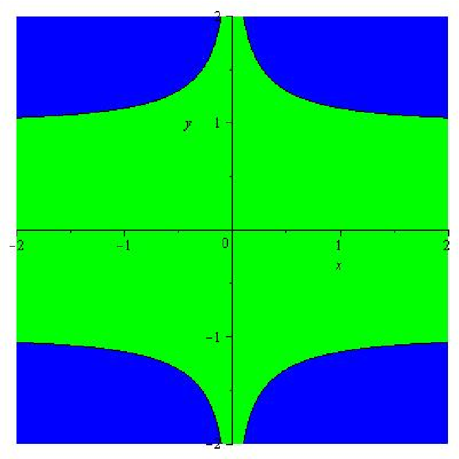
Let f=1+x4​y2+x​yf=1+x^{4}y^{2}+xy and g1=12+x2​y4−x2​y6g_{1}=\frac{1}{2}+x^{2}y^{4}-x^{2}y^{6}. The feasible set KK is a non-compact set depicted in Figure 1. Using Gloptipoly, one can check that −∞=fsos(4)-\infty=f_{\rm sos}^{(4)} and the optimal solution is given for d=8d=8 with fsos(8)≈0.4474f_{\rm sos}^{(8)}\approx 0.4474. In this case one can extract the minimizers (−0.557,1.2715)(-0.557,1.2715) and (0.557,−1.2715)(0.557,-1.2715).

We compare the results to our approach via geometric programming instead of Lasserre relaxations. From ff and g1g_{1} we get G⁡(μ)=(1−12​μ)+x4​y2+μ​x2​y6+x​y−μ​x2​y4G(\mu)=(1-\frac{1}{2}\mu)+x^{4}y^{2}+\mu x^{2}y^{6}+xy-\mu x^{2}y^{4}. Note that New⁡(G⁡(μ))\New(G(\mu)) is a two dimensional simplex if μ∉{0,2}\mu\notin\{0,2\}. Then, we have Δ⁡(G)={𝜷,𝜷~}={(1,1),(2,4)}\Delta(G)=\{\boldsymbol{\beta},\tilde{\boldsymbol{\beta}}\}=\{(1,1),(2,4)\}. Hence, we introduce the variables (a𝜷,1,a𝜷,2,a𝜷~,1,a𝜷~,2,b𝜷,b𝜷~,μ)(a_{\boldsymbol{\beta},1},a_{\boldsymbol{\beta},2},a_{\tilde{\boldsymbol{\beta}},1},a_{\tilde{\boldsymbol{\beta}},2},b_{\boldsymbol{\beta}},b_{\tilde{\boldsymbol{\beta}}},\mu). Therefore, the geometric program (3.2) reads as follows:

inf{12​μ+710⋅b𝜷107⋅(15)27⋅(110)17⋅(a𝜷,1)−27⋅(a𝜷,2)−17+15⋅b𝜷~5⋅(15)1⋅(35)3⋅(a𝜷~,1)−1⋅(a𝜷~,2)−3}\displaystyle\inf\left\{\frac{1}{2}\mu+\frac{7}{10}\cdot b_{\boldsymbol{\beta}}^{\frac{10}{7}}\cdot\left(\frac{1}{5}\right)^{\frac{2}{7}}\cdot\left(\frac{1}{10}\right)^{\frac{1}{7}}\cdot(a_{\boldsymbol{\beta},1})^{-\frac{2}{7}}\cdot(a_{\boldsymbol{\beta},2})^{-\frac{1}{7}}+\frac{1}{5}\cdot b_{\tilde{\boldsymbol{\beta}}}^{5}\cdot\left(\frac{1}{5}\right)^{1}\cdot\left(\frac{3}{5}\right)^{3}\cdot(a_{\tilde{\boldsymbol{\beta}},1})^{-1}\cdot(a_{\tilde{\boldsymbol{\beta}},2})^{-3}\right\}

such that the variables satisfy

a𝜷,1+a𝜷~,1≤1,a𝜷,2+a𝜷~,2≤μ​ and ​ 1≤b𝜷,μ≤b𝜷~.\displaystyle a_{\boldsymbol{\beta},1}+a_{\tilde{\boldsymbol{\beta}},1}\leq 1,\;a_{\boldsymbol{\beta},2}+a_{\tilde{\boldsymbol{\beta}},2}\leq\mu\;\text{ and }\;1\leq b_{\boldsymbol{\beta}},\;\mu\leq b_{\tilde{\boldsymbol{\beta}}}\;.

We use the Matlab solver CVX to solve the program given above. The optimal solution is given by

(a𝜷,1,a𝜷,2,a𝜷~,1,a𝜷~,2,b𝜷,b𝜷~,μ)=(0.9105,0.0540,0.0895,0.0319,1.0000,0.0859,0.0859).(a_{\boldsymbol{\beta},1},a_{\boldsymbol{\beta},2},a_{\tilde{\boldsymbol{\beta}},1},a_{\tilde{\boldsymbol{\beta}},2},b_{\boldsymbol{\beta}},b_{\tilde{\boldsymbol{\beta}}},\mu)\ =\ (0.9105,0.0540,0.0895,0.0319,1.0000,0.0859,0.0859)\;.

This leads to

γsonc≈ 0.5526\gamma_{\rm sonc}\ \approx\ 0.5526

and hence f𝜶⁡(0)−γsonc≈0.4474f_{\boldsymbol{\alpha}(0)}-\gamma_{\rm sonc}\approx 0.4474. Thus, we have

fsos(8)=f𝜶⁡(0)−γsonc=s⁡(f,g1).f^{(8)}_{\rm sos}\ =\ f_{\boldsymbol{\alpha}(0)}-\gamma_{\rm sonc}\ =\ s(f,g_{1}).

The equality f𝜶⁡(0)−γsonc=s⁡(f,g1)f_{\boldsymbol{\alpha}(0)}-\gamma_{\rm sonc}=s(f,g_{1}) is not surprising, since the assumptions of Theorem 3.5 are satisfied. Thus, we get the optimal solution immediately via geometric programming whereas one needs 55 relaxation steps via Lasserre relaxation. In this example both geometric programing and the Lasserre approach have a runtime below 1 second.

Now, we demonstrate that our approach, in contrast to SDPs, is not sensitive to increasing the degree, since it is based on GPs. Namely, if we multiply all exponents in ff and g1g_{1} by 10, then the approaches differ significantly. By multiplying the exponents by 10 we have made a severe change to the problem since the term x10​y10x^{10}y^{10} is now a monomial square such that the exponent is a lattice point in the interior of the Newton polytope of the adjusted G⁡(μ)G(\mu). Therefore, we have to ignore this term out when running the constrained optimization program (3.2). The adjusted program yields with CVX an output NaN in below one second. However, the reason is that it computes μ=0\mu=0, which is the correct answer. Namely, after multiplying the exponents by 10, the only non monomial square terms are given by g1g_{1}. Thus, the optimal choice is μ=0\mu=0, and we can see that the minimal value is attained at (0,0)(0,0) and fK∗=1f_{K}^{*}=1 is given by the constant term of ff.

In comparison, we have a runtime of approximately 11101110 seconds, i.e. approximately 18.518.5 minutes with Gloptipoly. After this time Gloptipoly provides an output “Run into numerical problems.”. It claims, however, to have solved the problem and provides the correct minimum fK∗=1f_{K}^{*}=1 at a minimizer 10−7⋅(−0.1057,0.1711)10^{-7}\cdot(-0.1057,0.1711), which, of course, is the origin up to a numerical error.

We remark that this particular artificial increase of the degree can, of course, be handled with SDP methods using pre-processing methods, e.g. a change of variables. The purpose of the rescaling of this and later examples is, however, to show that SONC/GP methods are inherently not sensitive to an increase of the degree. ⎔\hexagon
Refer to caption

Figure 1. The feasible set for the constrained optimization problem in Example 4.2 is the unbounded green (light) area.
Example 4.3.

Let f=1+x2​z2+y2​z2+x2​y2−8​x​y​zf=1+{x}^{2}{z}^{2}+{y}^{2}{z}^{2}+{x}^{2}{y}^{2}-8xyz and g1=x2​y​z+x​y2​z+x2​y2−2+x​y​zg_{1}={x}^{2}yz+x{y}^{2}z+{x}^{2}{y}^{2}-2+xyz. Using Gloptipoly, we get the following sequence of lower bounds:

fsos(2)=fsos(3)=fsos(4)=−∞<fsos(5)≈−14.999.f_{\rm sos}^{(2)}=f_{\rm sos}^{(3)}=f_{\rm sos}^{(4)}=-\infty<f_{\rm sos}^{(5)}\approx-14.999.

However, one cannot certify the optimality via Gloptipoly in this case. Additionally, the sequence fsos(d)f_{\rm sos}^{(d)} is not guaranteed to converge to fK∗f_{K}^{*}, since KK is unbounded. Symbolically, we were able to prove a global minimum of fK∗=−15f_{K}^{*}=-15 with four global minimizers (2,2,2),(−2,−2,2),(−2,2,−2),(2,−2,−2)(2,2,2),(-2,-2,2),(-2,2,-2),(2,-2,-2) using the quantifier elimination software Synrac, see [AY03]. Now, we consider the approach via geometric programming instead of Lasserre relaxations. We have

G⁡(μ)=(1+2​μ)+x2​z2+y2​z2+(1−μ)​x2​y2+(−8−μ)​x​y​z−μ​x2​y​z−μ​x​y2​z.G(\mu)\ =\ (1+2\mu)+x^{2}z^{2}+y^{2}z^{2}+(1-\mu)x^{2}y^{2}+(-8-\mu)xyz-\mu x^{2}yz-\mu xy^{2}z.

Therefore, G⁡(μ)G(\mu) is an ST-polynomial for μ∈[0,1)\mu\in[0,1), and we have Δ⁡(G)={𝜷,𝜷¯,𝜷^}=\Delta(G)=\{\boldsymbol{\beta},\overline{\boldsymbol{\beta}},\hat{\boldsymbol{\beta}}\}= {(1,1,1),(2,1,1),(1,2,1)}\{(1,1,1),(2,1,1),(1,2,1)\}. Thus, our geometric program has the following 13 variables

(a𝜷,1,a𝜷,2,a𝜷,3,a𝜷¯,1,a𝜷¯,2,a𝜷¯,3,a𝜷^,1,a𝜷^,2,a𝜷^,3,b𝜷,b𝜷¯,b𝜷^,μ).(a_{\boldsymbol{\beta},1},a_{\boldsymbol{\beta},2},a_{\boldsymbol{\beta},3},a_{\overline{\boldsymbol{\beta}},1},a_{\overline{\boldsymbol{\beta}},2},a_{\overline{\boldsymbol{\beta}},3},a_{\hat{\boldsymbol{\beta}},1},a_{\hat{\boldsymbol{\beta}},2},a_{\hat{\boldsymbol{\beta}},3},b_{\boldsymbol{\beta}},b_{\overline{\boldsymbol{\beta}}},b_{\hat{\boldsymbol{\beta}}},\mu).

Hence, program (3.2) is of the form

inf{0⋅μ+14⋅b𝜷4⋅(14)⋅(14)⋅(14)⋅(a𝜷,1)−1⋅(a𝜷,2)−1⋅(a𝜷,3)−1}\displaystyle\inf\left\{0\cdot\mu+\frac{1}{4}\cdot b_{\boldsymbol{\beta}}^{4}\cdot\left(\frac{1}{4}\right)\cdot\left(\frac{1}{4}\right)\cdot\left(\frac{1}{4}\right)\cdot(a_{\boldsymbol{\beta},1})^{-1}\cdot(a_{\boldsymbol{\beta},2})^{-1}\cdot(a_{\boldsymbol{\beta},3})^{-1}\right\}

such that

(1)a𝜷,1+a𝜷¯,1+a𝜷^,1≤1,a𝜷,2+a𝜷¯,2+a𝜷^,2≤1,a𝜷,3+a𝜷¯,3+a𝜷^,3+μ≤1,(2)12⋅b𝜷¯⋅(a𝜷¯,1)−12⋅(a𝜷¯,3)−12≤1,12⋅b𝜷^⋅(a𝜷^,2)−12⋅(a𝜷^,3)−12≤1,(3)8⋅b𝜷−1≤1,μ⋅b𝜷−1≤1,μ⋅b𝜷¯−1≤1,μ⋅b𝜷^−1≤1.\begin{array}[]{cl}(1)&a_{\boldsymbol{\beta},1}+a_{\overline{\boldsymbol{\beta}},1}+a_{\hat{\boldsymbol{\beta}},1}\leq 1,\ a_{\boldsymbol{\beta},2}+a_{\overline{\boldsymbol{\beta}},2}+a_{\hat{\boldsymbol{\beta}},2}\leq 1,\ a_{\boldsymbol{\beta},3}+a_{\overline{\boldsymbol{\beta}},3}+a_{\hat{\boldsymbol{\beta}},3}+\mu\leq 1,\\ (2)&\frac{1}{2}\cdot b_{\overline{\boldsymbol{\beta}}}\cdot\left(a_{\overline{\boldsymbol{\beta}},1}\right)^{-\frac{1}{2}}\cdot\left(a_{\overline{\boldsymbol{\beta}},3}\right)^{-\frac{1}{2}}\leq 1,\\ &\frac{1}{2}\cdot b_{\hat{\boldsymbol{\beta}}}\cdot\left(a_{\hat{\boldsymbol{\beta}},2}\right)^{-\frac{1}{2}}\cdot\left(a_{\hat{\boldsymbol{\beta}},3}\right)^{-\frac{1}{2}}\leq 1,\\ (3)&8\cdot b_{\boldsymbol{\beta}}^{-1}\leq 1,\ \mu\cdot b_{\boldsymbol{\beta}}^{-1}\leq 1,\ \mu\cdot b_{\overline{\boldsymbol{\beta}}}^{-1}\leq 1,\ \mu\cdot b_{\hat{\boldsymbol{\beta}}}^{-1}\leq 1\,.\end{array}

This leads to γsonc=1256⋅84=16\gamma_{\rm sonc}=\frac{1}{256}\cdot 8^{4}=16 and so f𝜶⁡(0)−γsonc=−15f_{\boldsymbol{\alpha}(0)}-\gamma_{\rm sonc}=-15. The runtime for this example is below 1 second. Multiplying the exponents of ff and g1g_{1} by 10 yields the same results; the runtime for the geometric program remains below 1 second. In comparison, Gloptipoly yields

fsos(d)=−∞​ for ​d≤19,f_{\rm sos}^{(d)}\ =\ -\infty\text{ for }d\leq 19,

and provides a bound

fsos(20)≈−14.999f_{\rm sos}^{(20)}\ \approx\ -14.999

in the 20-th relaxation after 3656336563 seconds, i.e. approximately 10.16 hours. Moreover, although this bound is numerically equal to fK∗f_{K}^{*}, Gloptipoly was not able to certify that the correct bound was found. ⎔\hexagon

Example 4.4.

Let f=z6+x4​y2+x2​y4−3​x2​y2​z2f=z^{6}+x^{4}y^{2}+x^{2}y^{4}-3x^{2}y^{2}z^{2} and g1=x2+y2+z2−1g_{1}=x^{2}+y^{2}+z^{2}-1. We obtain G⁡(μ)=f−μ​g1G(\mu)=f-\mu g_{1}. This problem is infeasible in the sense of program (3.2). Namely, condition (♣)(\clubsuit) is never satisfied since for any μ>0\mu>0 we have a vertex (2,0,0)(2,0,0) or (0,2,0)(0,2,0) of New⁡(G⁡(μ)){\rm New}(G(\mu)) with a negative coefficient. Therefore, one can immediately conclude that s⁡(f,g1)s(f,g_{1}) has to be obtained for μ=0\mu=0. Thus, we have s⁡(f,g1)=fsoncs(f,g_{1})=f_{\rm sonc}. Since ff is the homogenized Motzkin polynomial we obtain immediately fsonc=fK∗=0f_{\rm sonc}=f_{K}^{*}=0. An analogous argumentation holds for the variation G~​(μ)=f+μ​g1\tilde{G}(\mu)=f+\mu g_{1}.

It is well-known that SDP solvers have serious issues with optimizing ff for g1≥0g_{1}\geq 0 or g1≤0g_{1}\leq 0. For further information see [Nie13b, Examples 5.3 and 5.4]. ⎔\hexagon

In the last example in this section we show that for special simplices our geometric programming approach coincides with the one in [GM13].

Example 4.5.

Suppose that New⁡(G⁡(𝝁))=conv⁡{0,2​d​𝐞1,…,2​d​𝐞n}\New(G(\boldsymbol{\mu}))=\conv\{0,2d\,\mathbf{e}_{1},\dots,2d\,\mathbf{e}_{n}\}. Hence, the Newton polytope is a 2​d2d-scaled standard simplex in ℝn\mathbb{R}^{n}, which is the case if the pure powers xj2​dx_{j}^{2d} for 1≤j≤n1\leq j\leq n are present in the polynomial ff or in the constrained polynomials gig_{i}. The corresponding polynomial G⁡(𝝁)G(\boldsymbol{\mu}) is an ST-polynomial; see Section 2.1. Indeed, all examples in [GM13, Example 4.8] are of that form and thus all of them are ST-polynomials.

In this case the program (2.6) coincides with the program (3) in [GM13]. One drawback of this setting is that the geometric programming bounds obtained from (2.6) are at most as good as the bound fsos(d)f_{\rm sos}^{(d)}. Namely, if the Newton polytope of a circuit polynomial is a scaled standard simplex, then it is nonnegative if and only if it is a sum of squares; see [IdW16a] for further details. Thus, if we are in the setting of Ghasemi and Marshall and G⁡(𝝁)G(\boldsymbol{\mu}) is nonnegative, then it is a sum of squares of degree at most 2​d2d which guarantees the existence of a decomposition in the sense of fsos(d)f^{(d)}_{\rm sos}; see (4.1).

However, as we have shown in the previous examples, in the case of our program (2.6) there exist also cases where the geometric programming bounds are better than fsos(d)f_{\rm sos}^{(d)}, since our approach is more general than in [GM13]. The reason is that the cones of sums of nonnegative circuit polynomials and sums of squares do not contain each other (but both of them are contained in the cone of nonnegative polynomials); see [IdW16a, Prop. 7.2].

⎔\hexagon

We point out that we make no assumption about the feasible set KK. In particular, it is not assumed to be compact as it is in the classical setting via Lasserre relaxations in order to guarantee convergence of the relaxations. However, the crucial point in our setting so far is that G⁡(𝝁)G(\boldsymbol{\mu}) has to be an ST-polynomial. In the following Section 5 we lay the foundation for the usage of our geometric programming approach also for non-ST-polynomials.

But even if G⁡(𝝁)G(\boldsymbol{\mu}) is not an ST-polynomial, then we can enforce it to be an ST-polynomial in the case of a compact KK. This can be achieved by adding a redundant constraint gs+1=x12​d+…+xn2​d+cg_{s+1}=x_{1}^{2d}+\ldots+x_{n}^{2d}+c for c∈ℝc\in\mathbb{R} to the feasible set KK. In consequence New⁡(G⁡(𝝁))\New(G(\boldsymbol{\mu})) is a 2​d2d-scaled standard simplex and by the previous example our approach coincides with the one in [GM13]. Hence, the Lasserre relaxation cannot be outperformed in quality anymore. However, our approach can still have the better runtime. It would be interesting to add other redundant inequalities to KK such that the corresponding bounds are better than the ones obtained via Lasserre relaxations. Unfortunately, no systematic way is known so far.

Furthermore, we consider in this paper numerical methods to certify nonnegativity of polynomials. Often it is desirable to obtain exact solutions, i.e. a symbolic certification. It would be interesting to find symbolic certificates from our provided numerical solution. For SOS polynomials this has been studied e.g. by Peyrl and Parrilo [PP08] and by Kaltofen, Li, Yang, and Zhi [KLYZ12].

5. Optimization for Non-ST-Polynomials

The goal of this section is to provide a first approach to tackle optimization problems (both constrained and unconstrained) which cannot be expressed as a single ST-polynomial using the methods developed in [IdW16a, IdW16b] and in Section 3 in this article. A more careful investigation of these general types of nonnegativity problems will be content of a follow-up article.

We start with the case of global nonnegativity for arbitrary polynomials via SONC certificates. We recall the following statement from [IdW16a, Definition 7.1 and Proposition 7.2], which immediately follows from Section 2.1.

Fact 5.1.

Let f∈ℝ⁡[𝐱]f\in\mathbb{R}[\mathbf{x}] and assume that there exist SONC polynomials g1,…,gkg_{1},\ldots,g_{k} and positive real numbers μ1,…,μk\mu_{1},\ldots,\mu_{k} such that f=∑i=1kμi​gif=\sum_{i=1}^{k}\mu_{i}g_{i}. Then ff is nonnegative.

Of course, if a SONC decomposition exists, then it is not obvious how to find it in general. For ST-polynomials we know that we can find a SONC decomposition via the geometric optimization problem described in Theorem 2.6. Thus, we investigate a general polynomial f∈ℝ⁡[𝐱]f\in\mathbb{R}[\mathbf{x}] supported on a set A⊂ℕnA\subset\mathbb{N}^{n} satisfying (♣)(\clubsuit). We denote

f\displaystyle f =\displaystyle= ∑j=0df𝜶⁡(j)​𝐱𝜶⁡(j)+∑𝜷∈Δ⁡(f)f𝜷​𝐱𝜷\displaystyle\sum_{j=0}^{d}f_{\boldsymbol{\alpha}(j)}\mathbf{x}^{\boldsymbol{\alpha}(j)}+\sum_{\boldsymbol{\beta}\in\Delta(f)}f_{\boldsymbol{\beta}}\mathbf{x}^{\boldsymbol{\beta}}

such that f𝜶⁡(j)​𝐱𝜶⁡(j)f_{\boldsymbol{\alpha}(j)}\mathbf{x}^{\boldsymbol{\alpha}(j)} are monomial squares. By (♣)(\clubsuit), V⁡(A)V(A) are the vertices of New⁡(f)\New(f) and we have V⁡(A)⊆{𝜶⁡(0),…,𝜶⁡(d)}V(A)\subseteq\{\boldsymbol{\alpha}(0),\ldots,\boldsymbol{\alpha}(d)\}; equality, however, is not required here: {𝜶⁡(0),…,𝜶⁡(d)}\{\boldsymbol{\alpha}(0),\ldots,\boldsymbol{\alpha}(d)\} can also contain exponents of monomial squares in Δ⁡(A)∖Δ⁡(f)\Delta(A)\setminus\Delta(f) which are not vertices of conv⁡(A)\conv(A). For simplicity we assume in what follows that the affine span of AA is nn-dimensional. We proceed as follows:

  1. (1)

    Choose a triangulation T1,…,Tk{\color[rgb]{0.2,0.2,0.75}T_{1},\ldots,T_{k}} of exponents 𝜶⁡(0),…,𝜶⁡(d)∈A\boldsymbol{\alpha}(0),\ldots,\boldsymbol{\alpha}(d)\in A corresponding to the monomial squares.

  2. (2)

    Compute the induced covering A1,…,Ak{\color[rgb]{0.2,0.2,0.75}A_{1},\ldots,A_{k}} of AA given by Ai=A∩TiA_{i}=A\cap T_{i} for 1≤i≤k1\leq i\leq k.

  3. (3)

    Assume that 𝜷∈Δ⁡(f)⊂A\boldsymbol{\beta}\in\Delta(f)\subset A is contained in more than one of the AiA_{i}’s. Let without loss of generality 𝜷∈A1,…,Al\boldsymbol{\beta}\in A_{1},\ldots,A_{l} with 1<l≤k1<l\leq k. Then we choose f𝜷,1,…,f𝜷,l∈ℝ{\color[rgb]{0.2,0.2,0.75}f_{\boldsymbol{\beta},1},\ldots,f_{\boldsymbol{\beta},l}}\in\mathbb{R} such that ∑i=1lf𝜷,i=f𝜷\sum_{i=1}^{l}f_{\boldsymbol{\beta},i}=f_{\boldsymbol{\beta}} and sign⁡(f𝜷,i)=sign⁡(f𝜷)\sign(f_{\boldsymbol{\beta},i})=\sign(f_{\boldsymbol{\beta}}) for all 1≤i≤l1\leq i\leq l. We proceed analogously for 𝜶⁡(0),…,𝜶⁡(d)\boldsymbol{\alpha}(0),\ldots,\boldsymbol{\alpha}(d).

  4. (4)

    Define new polynomials g1,…,gkg_{1},\ldots,g_{k} such that

    gi\displaystyle{\color[rgb]{0.2,0.2,0.75}g_{i}} =\displaystyle= ∑𝜷∈Aif𝜷,i​𝐱𝜷.\displaystyle\sum_{\boldsymbol{\beta}\in A_{i}}f_{\boldsymbol{\beta},i}\mathbf{x}^{\boldsymbol{\beta}}.

Note that by (1) and (2) the covering AiA_{i} is a set of integer tuples such that conv⁡(Ai)\conv(A_{i}) is a simplex with even vertices and AiA_{i} contains no even points corresponding to monomial squares except for the vertices of conv⁡(Ai)\conv(A_{i}). Thus, by (2)–(4) we see that all gig_{i} are ST-polynomials, since the signs of the f𝜷,if_{\boldsymbol{\beta},i} are identical with the signs of the coefficients of ff. Therefore, monomial squares f𝜶⁡(j)​𝐱𝜶⁡(j)f_{\boldsymbol{\alpha}(j)}\mathbf{x}^{\boldsymbol{\alpha}(j)} of ff get decomposed into a sum of monomial squares ∑i=1kf𝜶⁡(j),i​𝐱𝜶⁡(j)\sum_{i=1}^{k}f_{\boldsymbol{\alpha}(j),i}\mathbf{x}^{\boldsymbol{\alpha}(j)} such that each individual monomial square f𝜶⁡(j),i​𝐱𝜶⁡(j)f_{\boldsymbol{\alpha}(j),i}\mathbf{x}^{\boldsymbol{\alpha}(j)} is a term of exactly one gig_{i}. We proceed analogously for the terms f𝜷​𝐱𝜷f_{\boldsymbol{\beta}}\mathbf{x}^{\boldsymbol{\beta}}. Additionally, it follows by construction that f=∑i=1kgif=\sum_{i=1}^{k}g_{i}. We apply the GP proposed in Corollary 2.7 on each of the gig_{i} with respect to a monomial square f𝜶⁡(j),i​𝐱𝜶⁡(j)f_{\boldsymbol{\alpha}(j),i}\mathbf{x}^{\boldsymbol{\alpha}(j)}, which is a vertex of New⁡(gi)=conv⁡(Ai)\New(g_{i})=\conv(A_{i}) (not necessarily the same 𝜶⁡(j)\boldsymbol{\alpha}(j) for every gig_{i}); we denote the minimizer by mi∗{\color[rgb]{0.2,0.2,0.75}m^{*}_{i}}. We make the following observation about these minimizers which was similarly already pointed out in [IdW16a, Section 3]:

Lemma 5.2.

Let f∈ℝ⁡[𝐱]f\in\mathbb{R}[\mathbf{x}] be a nonnegative circuit polynomial. Let b𝛂​𝐱𝛂b_{\boldsymbol{\alpha}}\mathbf{x}^{\boldsymbol{\alpha}} be a monomial with b𝛂>0b_{\boldsymbol{\alpha}}>0 and 𝛂∈(2​ℤ)n\boldsymbol{\alpha}\in(2\mathbb{Z})^{n}. Then b𝛂​𝐱𝛂⋅fb_{\boldsymbol{\alpha}}\mathbf{x}^{\boldsymbol{\alpha}}\cdot f is also a nonnegative circuit polynomial.

Note particularly that if 𝐯∈(ℝ∗)n\mathbf{v}\in(\mathbb{R}^{*})^{n} satisfies f⁡(𝐯)=0f(\mathbf{v})=0, then (b𝜶​𝐱𝜶⋅f)​(𝐯)=0(b_{\boldsymbol{\alpha}}\mathbf{x}^{\boldsymbol{\alpha}}\cdot f)(\mathbf{v})=0.

Proof.

It is easy to see that all conditions for (♣)(\clubsuit) as well as the conditions (ST1) and (ST2) remain valid for b𝜶​𝐱𝜶⋅fb_{\boldsymbol{\alpha}}\mathbf{x}^{\boldsymbol{\alpha}}\cdot f. Thus, b𝜶​𝐱𝜶⋅fb_{\boldsymbol{\alpha}}\mathbf{x}^{\boldsymbol{\alpha}}\cdot f still is a circuit polynomial and since b𝜶​𝐱𝜶≥0b_{\boldsymbol{\alpha}}\mathbf{x}^{\boldsymbol{\alpha}}\geq 0 it is also nonnegative. ∎

Proposition 5.3.

Let ff, g1,…,gkg_{1},\ldots,g_{k}, and mi∗m^{*}_{i} be as explained above. Assume for i=1,…,ki=1,\ldots,k that mi∗m^{*}_{i} corresponds to the monomial square f𝛂⁡(j),i​𝐱𝛂⁡(ji)f_{\boldsymbol{\alpha}(j),i}\mathbf{x}^{\boldsymbol{\alpha}(j_{i})} with 𝛂⁡(ji)∈{𝛂⁡(1),…,𝛂⁡(d)}∩V⁡(Ai)\boldsymbol{\alpha}(j_{i})\in\{\boldsymbol{\alpha}(1),\ldots,\boldsymbol{\alpha}(d)\}\cap V(A_{i}). Then f−∑i=1kmi∗​𝐱𝛂⁡(ji)f-\sum_{i=1}^{k}m^{*}_{i}\mathbf{x}^{\boldsymbol{\alpha}(j_{i})} is a SONC and hence nonnegative. Thus, the mi∗m^{*}_{i} provide bounds for the coefficients f𝛂⁡(j),if_{\boldsymbol{\alpha}(j),i} for ff to be nonnegative. Particularly, if for i=1,…,li=1,\ldots,l with l≤kl\leq k the exponents 𝛂⁡(ji)\boldsymbol{\alpha}(j_{i}) are the origin, then f𝛂⁡(0)−∑i=1lmi∗f_{\boldsymbol{\alpha}(0)}-\sum_{i=1}^{l}m^{*}_{i} is a lower bound for f∗=sup{γ∈ℝ|f−γ≥0}{\color[rgb]{0.2,0.2,0.75}f^{*}}=\sup\{\gamma\in\mathbb{R}\ |\ f-\gamma\geq 0\}.

Proof.

By construction, we know that gi−mi∗​𝐱𝜶⁡(ji)g_{i}-m^{*}_{i}\mathbf{x}^{\boldsymbol{\alpha}(j_{i})} is a SONC. Thus, f−∑i=1kmi∗​𝐱𝜶⁡(ji)=∑i=1kgi−mi∗​𝐱𝜶⁡(ji)f-\sum_{i=1}^{k}m^{*}_{i}\mathbf{x}^{\boldsymbol{\alpha}(j_{i})}=\sum_{i=1}^{k}g_{i}-m^{*}_{i}\mathbf{x}^{\boldsymbol{\alpha}(j_{i})} is a SONC, too. The last part follows by the definitions of the mi∗m_{i}^{*}’s and f∗f^{*}. ∎

Note that the decomposition of ff into the gig_{i}’s is not unique. First, the triangulation in (1) is not unique in general. And, second, the decomposition of the terms in (3) is arbitrary. Note also that there exist several monomial squares which appear in more than one gig_{i}, since membership in AiA_{i} is given by the chosen triangulation and every simplex T1T_{1} intersects at least one other simplex T2T_{2} in an n−1n-1 dimensional face, which means that A1∩A2A_{1}\cap A_{2} contains at least nn even elements. As mentioned in the introduction, the problem to identify an optimal triangulation and an optimal decomposition of coefficients will be discussed in a follow-up article.

We provide some examples to show how this generalized approach can be used in practice.

Example 5.4.

Let f=6+x12​x26+2​x14​x26+1​x18​x22−1.2​x12​x23−0.85​x13​x25−0.9​x14​x23−0.73​x15​x22−1.14​x17​x22f=6+x_{1}^{2}x_{2}^{6}+2x_{1}^{4}x_{2}^{6}+1x_{1}^{8}x_{2}^{2}-1.2x_{1}^{2}x_{2}^{3}-0.85x_{1}^{3}x_{2}^{5}-0.9x_{1}^{4}x_{2}^{3}-0.73x_{1}^{5}x_{2}^{2}-1.14x_{1}^{7}x_{2}^{2}. We choose a triangulation

{(𝟎,𝟎),(𝟐,𝟔),(𝟒,𝟔),(2,3),(3,5)},{(𝟎,𝟎),(𝟒,𝟔),(𝟖,𝟐),(2,3),(4,3),(5,2),(7,2)}.\displaystyle\{{\color[rgb]{1,0,0}\mathbf{(0,0)}},{\color[rgb]{1,0,0}\mathbf{(2,6)}},{\color[rgb]{1,0,0}\mathbf{(4,6)}},(2,3),(3,5)\},\{{\color[rgb]{1,0,0}\mathbf{(0,0)}},{\color[rgb]{1,0,0}\mathbf{(4,6)}},{\color[rgb]{1,0,0}\mathbf{(8,2)}},(2,3),(4,3),(5,2),(7,2)\}.

Here and in what follows the vertices of each simplex are printed in red (bold). For the corresponding Newton polytope see Figure 2. We split the coefficients equally among the two triangulations and obtain two ST-polynomials

g1\displaystyle g_{1} =\displaystyle= 3+x12​x26+x14​x26−0.6​x12​x23−0.85​x13​x25, and\displaystyle 3+x_{1}^{2}x_{2}^{6}+x_{1}^{4}x_{2}^{6}-0.6x_{1}^{2}x_{2}^{3}-0.85x_{1}^{3}x_{2}^{5},\text{ and }
g2\displaystyle g_{2} =\displaystyle= 3+x14​x26+1​x18​x22−0.6​x12​x23−0.9​x14​x23−0.73​x15​x22−1.14​x17​x22.\displaystyle 3+x_{1}^{4}x_{2}^{6}+1x_{1}^{8}x_{2}^{2}-0.6x_{1}^{2}x_{2}^{3}-0.9x_{1}^{4}x_{2}^{3}-0.73x_{1}^{5}x_{2}^{2}-1.14x_{1}^{7}x_{2}^{2}.

Using CVX, we apply the GP from Corollary 2.7 and obtain optimal values m1∗=0.2121m_{1}^{*}=0.2121, m2∗=2.5193m_{2}^{*}=2.5193, and a SONC decomposition

0.173+ε​x12​x26+0.522​x14​x26−0.6​x12​x23+0.04+x12​x26+0.478​x14​x26−0.85​x13​x25+0.427+0.211​x14​x26+ε​x18​x22−0.6​x12​x23+0.663+0.436​x14​x26+0.085​x18​x22−0.9​x14​x23+0.753+0.186​x14​x26+0.177​x18​x22−0.73​x15​x22+0.676+0.167​x14​x26+0.738​x18​x22−1.14​x17​x22,\displaystyle\begin{array}[]{lclc}0.173+\varepsilon x_{1}^{2}x_{2}^{6}+0.522x_{1}^{4}x_{2}^{6}-0.6x_{1}^{2}x_{2}^{3}&+&0.04+x_{1}^{2}x_{2}^{6}+0.478x_{1}^{4}x_{2}^{6}-0.85x_{1}^{3}x_{2}^{5}&+\\ 0.427+0.211x_{1}^{4}x_{2}^{6}+\varepsilon x_{1}^{8}x_{2}^{2}-0.6x_{1}^{2}x_{2}^{3}&+&0.663+0.436x_{1}^{4}x_{2}^{6}+0.085x_{1}^{8}x_{2}^{2}-0.9x_{1}^{4}x_{2}^{3}&+\\ 0.753+0.186x_{1}^{4}x_{2}^{6}+0.177x_{1}^{8}x_{2}^{2}-0.73x_{1}^{5}x_{2}^{2}&+&0.676+0.167x_{1}^{4}x_{2}^{6}+0.738x_{1}^{8}x_{2}^{2}-1.14x_{1}^{7}x_{2}^{2},&\\ \end{array}

with ε<10−10\varepsilon<10^{-10}, i.e. ε\varepsilon is numerically zero. Namely, (2,3)(2,3) is located on the segment given by (𝟎,𝟎){\color[rgb]{1,0,0}\mathbf{(0,0)}} and (𝟒,𝟔){\color[rgb]{1,0,0}\mathbf{(4,6)}} and thus (𝟐,𝟔){\color[rgb]{1,0,0}\mathbf{(2,6)}} and (𝟖,𝟐){\color[rgb]{1,0,0}\mathbf{(8,2)}} have coefficients zero in the convex combinations of the point (2,3)(2,3).

Thus, the optimal value fsoncf_{\rm sonc}, which provides us a lower bound for f∗f^{*}, is fsonc≈6−2.731=3.269f_{\rm sonc}\approx 6-2.731=3.269. In comparison, via Lasserre relaxation one obtains an only slightly better optimal value f∗=3.8673f^{*}=3.8673.

Our GP based bound can be improved significantly via making small changes in the distribution of the coefficients. For example, if one decides not to split the coefficient of the term x12​x23x_{1}^{2}x_{2}^{3} among g1g_{1} and g2g_{2} equally, but to put the entire weight of the coefficient into g1g_{1}, i.e.,

g~1\displaystyle\tilde{g}_{1} =\displaystyle= 3+x12​x26+x14​x26−1.2​x12​x23−0.85​x13​x25, and\displaystyle 3+x_{1}^{2}x_{2}^{6}+x_{1}^{4}x_{2}^{6}-1.2x_{1}^{2}x_{2}^{3}-0.85x_{1}^{3}x_{2}^{5},\text{ and }
g~2\displaystyle\tilde{g}_{2} =\displaystyle= 3+x14​x26+1​x18​x22−0.9​x14​x23−0.73​x15​x22−1.14​x17​x22,\displaystyle 3+x_{1}^{4}x_{2}^{6}+1x_{1}^{8}x_{2}^{2}-0.9x_{1}^{4}x_{2}^{3}-0.73x_{1}^{5}x_{2}^{2}-1.14x_{1}^{7}x_{2}^{2},

then this yields to an improved bound f~sonc≈3.572\tilde{f}_{\rm sonc}\approx 3.572. ⎔\hexagon

Refer to caption
Refer to caption
Figure 2. The Newton polytopes of the polynomials in the Examples 5.4 and 5.5 and their triangulations.

The next example shows that we can use the approach of this section to take monomial squares into account, which are not vertices of the Newton polytope of the polynomial which we intend to minimize.

Example 5.5.

Let f=1+3​x12​x26+2​x16​x22+6​x12​x22−x1​x22−2​x12​x2−3​x13​x23f=1+3x_{1}^{2}x_{2}^{6}+2x_{1}^{6}x_{2}^{2}+6x_{1}^{2}x_{2}^{2}-x_{1}x_{2}^{2}-2x_{1}^{2}x_{2}-3x_{1}^{3}x_{2}^{3}. We choose a triangulation

{(𝟎,𝟎),(𝟐,𝟐),(𝟐,𝟔),(1,2)},{(𝟎,𝟎),(𝟐,𝟐),(𝟔,𝟐),(2,1)},{(𝟐,𝟐),(𝟐,𝟔),(𝟔,𝟐),(3,3)}.\displaystyle\{{\color[rgb]{1,0,0}\mathbf{(0,0)}},{\color[rgb]{1,0,0}\mathbf{(2,2)}},{\color[rgb]{1,0,0}\mathbf{(2,6)}},(1,2)\},\{{\color[rgb]{1,0,0}\mathbf{(0,0)}},{\color[rgb]{1,0,0}\mathbf{(2,2)}},{\color[rgb]{1,0,0}\mathbf{(6,2)}},(2,1)\},\{{\color[rgb]{1,0,0}\mathbf{(2,2)}},{\color[rgb]{1,0,0}\mathbf{(2,6)}},{\color[rgb]{1,0,0}\mathbf{(6,2)}},(3,3)\}.

For the corresponding Newton polytope see Figure 2. First, we split the coefficients equally among the three triangulations such that we obtain

g1\displaystyle g_{1} =\displaystyle= 0.5+1.5​x12​x26+2​x12​x22−x1​x22,\displaystyle 0.5+1.5x_{1}^{2}x_{2}^{6}+2x_{1}^{2}x_{2}^{2}-x_{1}x_{2}^{2},
g2\displaystyle g_{2} =\displaystyle= 0.5+1​x16​x22+2​x12​x22−2​x12​x2,\displaystyle 0.5+1x_{1}^{6}x_{2}^{2}+2x_{1}^{2}x_{2}^{2}-2x_{1}^{2}x_{2},
g3\displaystyle g_{3} =\displaystyle= 1.5​x12​x26+1​x16​x22+2​x12​x22−3​x13​x23.\displaystyle 1.5x_{1}^{2}x_{2}^{6}+1x_{1}^{6}x_{2}^{2}+2x_{1}^{2}x_{2}^{2}-3x_{1}^{3}x_{2}^{3}.

All three gig_{i} have a joint monomial x12​x22x_{1}^{2}x_{2}^{2}. For all i=1,2,3i=1,2,3 we compute the maximal bi>0b_{i}>0 such that gi−bi​x12​x22g_{i}-b_{i}x_{1}^{2}x_{2}^{2} is a nonnegative circuit polynomial. This yields a bound for the coefficient of x12​x22x_{1}^{2}x_{2}^{2} certifying that ff is a SONC and hence nonnegative. We could apply the GP from Corollary 2.7, but since all gig_{i} are circuit polynomials we can compute the corresponding circuit numbers symbolically. We obtain with Theorem 2.4:

Θg1​(1,2)\displaystyle\Theta_{g_{1}}(1,2) =\displaystyle= (1/21/2)12⋅(3/21/4)14⋅(2−b11/4)14=4⋅4⋅3/2⋅(2−b1)4= 2​3/2⋅(2−b1)4,\displaystyle\left(\frac{1/2}{1/2}\right)^{\frac{1}{2}}\cdot\left(\frac{3/2}{1/4}\right)^{\frac{1}{4}}\cdot\left(\frac{2-b_{1}}{1/4}\right)^{\frac{1}{4}}\ =\ \sqrt[4]{4\cdot 4\cdot 3/2\cdot(2-b_{1})}\ =\ 2\sqrt[4]{3/2\cdot(2-b_{1})},
Θg2​(2,1)\displaystyle\Theta_{g_{2}}(2,1) =\displaystyle= (1/41/2)12⋅(1/21/4)14⋅(1−1/2⋅b21/4)14=1/4⋅2⋅4​(1−1/2⋅b2)4=2−b24, and\displaystyle\left(\frac{1/4}{1/2}\right)^{\frac{1}{2}}\cdot\left(\frac{1/2}{1/4}\right)^{\frac{1}{4}}\cdot\left(\frac{1-1/2\cdot b_{2}}{1/4}\right)^{\frac{1}{4}}\ =\ \sqrt[4]{1/4\cdot 2\cdot 4(1-1/2\cdot b_{2})}\ =\ \sqrt[4]{2-b_{2}},\text{ and }
Θg3​(3,3)\displaystyle\Theta_{g_{3}}(3,3) =\displaystyle= (1/21/4)14⋅(1/31/4)14⋅(1/3​(2−b3)1/2)12=2⋅4/34⋅2/3⋅(2−b3)= 2​2/274​2−b3.\displaystyle\left(\frac{1/2}{1/4}\right)^{\frac{1}{4}}\cdot\left(\frac{1/3}{1/4}\right)^{\frac{1}{4}}\cdot\left(\frac{1/3(2-b_{3})}{1/2}\right)^{\frac{1}{2}}\ =\ \sqrt[4]{2\cdot 4/3}\cdot\sqrt{2/3\cdot(2-b_{3})}\ =\ 2\sqrt[4]{2/27}\sqrt{2-b_{3}}.

This provides solutions:

2​3/2⋅(2−b1)4≥ 1\displaystyle 2\sqrt[4]{3/2\cdot(2-b_{1})}\ \geq\ 1 ⇔\displaystyle\Leftrightarrow 3/2⋅(2−b1)≥ 1/16⇔b1≤ 47/24,\displaystyle 3/2\cdot(2-b_{1})\ \geq\ 1/16\ \Leftrightarrow\ b_{1}\ \leq\ 47/24,
2−b24≥ 1\displaystyle\sqrt[4]{2-b_{2}}\ \geq\ 1 ⇔\displaystyle\Leftrightarrow b2≤ 1,\displaystyle b_{2}\ \leq\ 1,
2​2/274​2−b3≥ 1\displaystyle 2\sqrt[4]{2/27}\sqrt{2-b_{3}}\ \geq\ 1 ⇔\displaystyle\Leftrightarrow 2/27⋅(2−b3)≥ 1/4⇔b3≤ 2−27/(2​2).\displaystyle\sqrt{2/27}\cdot(2-b_{3})\ \geq\ 1/4\ \Leftrightarrow\ b_{3}\ \leq\ 2-\sqrt{27}/(2\sqrt{2}).

Hence, we obtain the following bound for the coefficient of x12​x22x_{1}^{2}x_{2}^{2}:

6−(47/24+1+2−27/(4​2))\displaystyle 6-(47/24+1+2-\sqrt{27}/(4\sqrt{2})) ≈\displaystyle\approx 6−4.03977468≈ 1.96.\displaystyle 6-4.03977468\ \approx\ 1.96.

A double check with the CVX solver for GPs yields the same value in approximately 0.7530.753 seconds.

We want to compute a bound for f∗f^{*}. We choose the same triangulation and the same split of coefficients as before, but now we optimize the constant term in g1g_{1} and g2g_{2}, and we optimize the coefficient of x12​x26x_{1}^{2}x_{2}^{6} in g3g_{3}. After a runtime of approximately 0.66570.6657 seconds we obtain optimal values 0.0722,0.35360.0722,0.3536, and 0.31640.3164. Thus, we found a lower bound for the constant term given by

m1∗+m2∗\displaystyle m_{1}^{*}+m_{2}^{*} ≈\displaystyle\approx 0.0722+0.3536= 0.4268.\displaystyle 0.0722+0.3536\ =\ 0.4268.

The corresponding optimal SONC decomposition is given by

0.0722+1.5​x12​x26+2​x12​x22−x11​x22+0.3536+1​x16​x22+2​x12​x22−1​x12​x21+0.3164​x12​x26+1​x16​x22+2​x12​x22−3​x13​x23\displaystyle\begin{array}[]{lclc}0.0722+1.5x_{1}^{2}x_{2}^{6}+2x_{1}^{2}x_{2}^{2}-x_{1}^{1}x_{2}^{2}&+&0.3536+1x_{1}^{6}x_{2}^{2}+2x_{1}^{2}x_{2}^{2}-1x_{1}^{2}x_{2}^{1}&+\\ 0.3164x_{1}^{2}x_{2}^{6}+1x_{1}^{6}x_{2}^{2}+2x_{1}^{2}x_{2}^{2}-3x_{1}^{3}x_{2}^{3}&&&\\ \end{array}

Thus, we obtain a bound for f∗f^{*} given by

fsonc\displaystyle f_{\rm sonc} =\displaystyle= 1−0.4268= 0.5732\displaystyle 1-0.4268\ =\ 0.5732

We make a comparison and optimize ff with Lasserre relaxation. This yields an optimal value

fsos=f∗≈ 0.8383.f_{\rm sos}\ =\ f^{*}\ \approx\ 0.8383.

Therefore, we want to improve our bound. We keep the triangulation, but we use another distribution of the coefficients among the polynomials g1,g2g_{1},g_{2} and g3g_{3} and define instead

g~1\displaystyle\tilde{g}_{1} =\displaystyle= 0.25+2​x12​x26+1.217​x12​x22−2​x1​x22,\displaystyle 0.25+2x_{1}^{2}x_{2}^{6}+1.217x_{1}^{2}x_{2}^{2}-2x_{1}x_{2}^{2},
g~2\displaystyle\tilde{g}_{2} =\displaystyle= 0.75+1​x16​x22+3.652​x12​x22−1​x12​x2,\displaystyle 0.75+1x_{1}^{6}x_{2}^{2}+3.652x_{1}^{2}x_{2}^{2}-1x_{1}^{2}x_{2},
g~3\displaystyle\tilde{g}_{3} =\displaystyle= 1​x12​x26+1​x16​x22+1.13​x12​x22−3​x13​x23.\displaystyle 1x_{1}^{2}x_{2}^{6}+1x_{1}^{6}x_{2}^{2}+1.13x_{1}^{2}x_{2}^{2}-3x_{1}^{3}x_{2}^{3}.

Again, we optimize g~1\tilde{g}_{1} and g~2\tilde{g}_{2} with respect to the constant term and g~3\tilde{g}_{3} with respect to x12​x26x_{1}^{2}x_{2}^{6}. We obtain optimal values 0.0801,0.26160.0801,0.2616, and 0.99120.9912. Thus, we are able to improve our bound for f∗f^{*} to

f~sonc\displaystyle\tilde{f}_{\rm sonc} ≈\displaystyle\approx 1−(0.0801+0.2616)= 0.6583.\displaystyle 1-(0.0801+0.2616)\ =\ 0.6583.

The corresponding optimal SONC decomposition is given by

0.0801+2​x12​x26+1.205​x12​x22−2​x11​x22+0.2616+1​x16​x22+3.615​x12​x22−1​x12​x21+0.991​x12​x26+1​x16​x22+2​x12​x22−3​x13​x23.\displaystyle\begin{array}[]{lclc}0.0801+2x_{1}^{2}x_{2}^{6}+1.205x_{1}^{2}x_{2}^{2}-2x_{1}^{1}x_{2}^{2}&+&0.2616+1x_{1}^{6}x_{2}^{2}+3.615x_{1}^{2}x_{2}^{2}-1x_{1}^{2}x_{2}^{1}&+\\ 0.991x_{1}^{2}x_{2}^{6}+1x_{1}^{6}x_{2}^{2}+2x_{1}^{2}x_{2}^{2}-3x_{1}^{3}x_{2}^{3}.&&&\\ \end{array}

⎔\hexagon

Refer to caption
Refer to caption
Figure 3. The Newton polytopes of the polynomials in the Examples 5.6 and 5.7 and their triangulations.

We discuss a third example which shows that, in the case of global optimization, for the GP/SONC approach it is not necessary to optimize the constant term to obtain a bound for nonnegativity on the coefficients, but that in some cases it can be informative to focus on other vertices of the Newton polytope or on other monomial squares instead.

Example 5.6.

Let f=1+x14+x22+x12​x24+x14​x24−x1​x2−x1​x22−x12​x23−x13​x23f=1+x_{1}^{4}+x_{2}^{2}+x_{1}^{2}x_{2}^{4}+x_{1}^{4}x_{2}^{4}-x_{1}x_{2}-x_{1}x_{2}^{2}-x_{1}^{2}x_{2}^{3}-x_{1}^{3}x_{2}^{3}. We choose a triangulation

{(𝟎,𝟎),(𝟎,𝟐),(𝟒,𝟎),(1,1)},{(𝟎,𝟐),(𝟐,𝟒),(𝟒,𝟎),(1,2),(2,3)},{(𝟐,𝟒),(𝟒,𝟎),(𝟒,𝟒),(3,3)}.\displaystyle\{{\color[rgb]{1,0,0}\mathbf{(0,0)}},{\color[rgb]{1,0,0}\mathbf{(0,2)}},{\color[rgb]{1,0,0}\mathbf{(4,0)}},(1,1)\},\{{\color[rgb]{1,0,0}\mathbf{(0,2)}},{\color[rgb]{1,0,0}\mathbf{(2,4)}},{\color[rgb]{1,0,0}\mathbf{(4,0)}},(1,2),(2,3)\},\{{\color[rgb]{1,0,0}\mathbf{(2,4)}},{\color[rgb]{1,0,0}\mathbf{(4,0)}},{\color[rgb]{1,0,0}\mathbf{(4,4)}},(3,3)\}.

Again, we choose a decomposition of coefficients such that their values split equally. We obtain the following ST-polynomials

g1\displaystyle g_{1} =\displaystyle= 1+1/3⋅x14+1/2⋅x22−x1​x2,\displaystyle 1+1/3\cdot x_{1}^{4}+1/2\cdot x_{2}^{2}-x_{1}x_{2},
g2\displaystyle g_{2} =\displaystyle= 1/3⋅x14+1/2⋅x12​x24+1/2⋅x22−x1​x22−x12​x23,\displaystyle 1/3\cdot x_{1}^{4}+1/2\cdot x_{1}^{2}x_{2}^{4}+1/2\cdot x_{2}^{2}-x_{1}x_{2}^{2}-x_{1}^{2}x_{2}^{3},
g3\displaystyle g_{3} =\displaystyle= 1/3⋅x14+1/2⋅x12​x24+x14​x24−x13​x23.\displaystyle 1/3\cdot x_{1}^{4}+1/2\cdot x_{1}^{2}x_{2}^{4}+x_{1}^{4}x_{2}^{4}-x_{1}^{3}x_{2}^{3}.

g1g_{1} and g3g_{3} are circuit polynomials while g2g_{2} contains two negative terms. For the corresponding Newton polytope see Figure 3. Note that only the exponent (𝟒,𝟎){\color[rgb]{1,0,0}\mathbf{(4,0)}} is contained in the support of all three ST-polynomials. Since (𝟒,𝟎){\color[rgb]{1,0,0}\mathbf{(4,0)}} is a monomial square which is a vertex of the convex hull of the three support sets, we optimize the corresponding coefficient in g1,g2g_{1},g_{2} and g3g_{3}. Applying the GP from Corollary 2.7 yields optimal values

m1∗= 0.0625,m2∗= 4.2867,andm3∗= 0.0625.\displaystyle m_{1}^{*}\ =\ 0.0625,\quad m_{2}^{*}\ =\ 4.2867,\quad\text{and}\quad m_{3}^{*}\ =\ 0.0625.

Since m2∗=4.2867>1/3m_{2}^{*}=4.2867>1/3 we found no certificate of nonnegativity for ff. However, we find a SONC decomposition for ff if the coefficient b(4,0)b_{(4,0)} of x14x_{1}^{4} is at least m1∗+m2∗+m3∗=4.412m_{1}^{*}+m_{2}^{*}+m_{3}^{*}=4.412. For this minimal choice of b(4,0)b_{(4,0)} a SONC decomposition is given by

0.063​x14+1+0.5​x22−1​x11​x21+2.143​x14+0.4​x22+0.1​x12​x24−1​x11​x22+2.143​x14+0.1​x22+0.4​x12​x24−1​x12​x23+0.063​x14+0.5​x12​x24+1​x14​x24−1​x13​x23\displaystyle\begin{array}[]{lclc}0.063x_{1}^{4}+1+0.5x_{2}^{2}-1x_{1}^{1}x_{2}^{1}&+&2.143x_{1}^{4}+0.4x_{2}^{2}+0.1x_{1}^{2}x_{2}^{4}-1x_{1}^{1}x_{2}^{2}&+\\ 2.143x_{1}^{4}+0.1x_{2}^{2}+0.4x_{1}^{2}x_{2}^{4}-1x_{1}^{2}x_{2}^{3}&+&0.063x_{1}^{4}+0.5x_{1}^{2}x_{2}^{4}+1x_{1}^{4}x_{2}^{4}-1x_{1}^{3}x_{2}^{3}&\\ \end{array}

⎔\hexagon

Finally, we apply the new method to a constrained optimization problem using the methods developed in Section 3.

Example 5.7.

Let f=1+x4+x2​y4f=1+x^{4}+x^{2}y^{4} and g=12+x2​y−x6​y4−x3​y3g=\frac{1}{2}+x^{2}y-x^{6}y^{4}-x^{3}y^{3}. Hence, we obtain G⁡(μ)=(1−12​μ)+x4+x2​y4+μ​x6​y4−μ​x2​y+μ​x3​y3G(\mu)=(1-\frac{1}{2}\mu)+x^{4}+x^{2}y^{4}+\mu x^{6}y^{4}-\mu x^{2}y+\mu x^{3}y^{3}. Choosing the triangulation

{(𝟎,𝟎),(𝟒,𝟎),(𝟔,𝟒),(2,1)},{(𝟎,𝟎),(𝟔,𝟒),(𝟐,𝟒),(3,3)},\displaystyle\{{\color[rgb]{1,0,0}\mathbf{(0,0)}},{\color[rgb]{1,0,0}\mathbf{(4,0)}},{\color[rgb]{1,0,0}\mathbf{(6,4)}},(2,1)\},\{{\color[rgb]{1,0,0}\mathbf{(0,0)}},{\color[rgb]{1,0,0}\mathbf{(6,4)}},{\color[rgb]{1,0,0}\mathbf{(2,4)}},(3,3)\},

we split the coefficients again, such that their values are equal. For the corresponding Newton polytope see Figure 3. We obtain the ST-polynomials

G1​(μ)\displaystyle G_{1}(\mu) =\displaystyle= (12−14​μ)+x4+12​μ​x6​y4−μ​x2​y,\displaystyle\left(\frac{1}{2}-\frac{1}{4}\mu\right)+x^{4}+\frac{1}{2}\mu x^{6}y^{4}-\mu x^{2}y,
G2​(μ)\displaystyle G_{2}(\mu) =\displaystyle= (12−14​μ)+x2​y4+12​μ​x6​y4+μ​x3​y3.\displaystyle\left(\frac{1}{2}-\frac{1}{4}\mu\right)+x^{2}y^{4}+\frac{1}{2}\mu x^{6}y^{4}+\mu x^{3}y^{3}.

Therefore, we see that the possible μ\mu values to obtain ST-polynomials are μ∈[0,2)\mu\in[0,2). We optimize both polynomials with respect to the constant term and obtain m1∗=m2∗=0m^{*}_{1}=m^{*}_{2}=0. The CVX solver yields NaN as an optimal value, since 0 is not positive. However, it solves the problem and computes values 00 or ε<10−200\varepsilon<10^{-200} for all variables, such that m1∗=m2∗=0m^{*}_{1}=m^{*}_{2}=0 follows. Hence, f𝜶⁡(0)−m∗=1−0=1f_{\boldsymbol{\alpha}(0)}-m^{*}=1-0=1 and because all of the assumptions in Theorem 3.5 are satisfied we know s⁡(f,g)=1s(f,g)=1.

Checking this optimization problem with Lasserre relaxation, we get fsos=fK∗=1f_{\rm sos}=f_{K}^{*}=1, which approves the optimal value. Both, for the SDP and the GP we have runtimes below 1 second.

Now, we tackle the same problem, but we multiply every exponent by 10, and we compare the runtimes again. For the GP we obtain the same result and the runtime remains below 1 second. For the SDP we obtain with Gloptipoly fsos=fK∗=1f_{\rm sos}=f_{K}^{*}=1 in approximately 5034.5\mathbf{5034.5} seconds, i.e. approximately 1.4\mathbf{1.4} hours.

In a third approach we tackle the same problem, but we multiply the originally given exponents by 20. In this case Gloptipoly is not able to handle the given matrices anymore. In comparison, we still have a runtime below 1 second for our GP providing the same bound as before.

Now, we also re-compute the example with the software SOSTOOLS [PAV+13], which, in contrast to Gloptipoly, can exploit sparsity patterns. For the original problem size, the runtime is 0.42 seconds, but already in the case that all exponents are multiplied by 10 we have a runtime of 302.7100 seconds, i.e. about 5 minutes.

Finally, we make a last comparison using the software SparsePOP [WKK+09], which especially serves to compute sparse problems based on SOS. Here we start with a runtime of 0.4495 seconds for the original problem. For the case of all exponents of ff multiplied by 1010 we get a runtime of 81.5438 seconds, i.e. 1.359 minutes. ⎔\hexagon

References

  • [AY03] H. Anai and H. Yanami, SyNRAC: a Maple-package for solving real algebraic constraints, Computational science—ICCS 2003. Part I, Lecture Notes in Comput. Sci., vol. 2657, Springer, Berlin, 2003, pp. 828–837.
  • [BG08] S. Boyd and M. Grant, Graph implementations for nonsmooth convex programs, Recent Advances in Learning and Control (V. Blondel, S. Boyd, and H. Kimura, eds.), Lecture Notes in Control and Information Sciences, Springer-Verlag Limited, 2008, http://stanford.edu/~boyd/graph_dcp.html, pp. 95–110.
  • [BGY06] S. Boyd, M. Grant, and Y. Ye, Disciplined convex programming, Global optimization, Nonconvex Optim. Appl., vol. 84, Springer, New York, 2006, pp. 155–210.
  • [BKVH07] S. Boyd, S.J. Kim, L. Vandenberghe, and A. Hassibi, A tutorial on geometric programming, Optim. Eng. 8 (2007), no. 1, 67–127.
  • [Ble06] G. Blekherman, There are significantly more nonnegative polynomials than sums of squares, Israel J. Math. 153 (2006), 355–380.
  • [Ble12] by same author, Nonnegative polynomials and sums of squares, J. Amer. Math. Soc. 25 (2012), no. 3, 617–635.
  • [BPT13] G. Blekherman, P.A. Parrilo, and R.R. Thomas, Semidefinite optimization and convex algebraic geometry, MOS-SIAM Series on Optimization, vol. 13, SIAM and the Mathematical Optimization Society, Philadelphia, 2013.
  • [BV04] S. Boyd and L. Vandenberghe, Convex optimization, Cambridge University Press, Cambridge, 2004.
  • [DG14] P.J.C. Dickinson and L. Gijben, On the computational complexity of membership problems for the completely positive cone and its dual, Comput. Optim. Appl. 57 (2014), no. 2, 403–415.
  • [dKL10] E. de Klerk and M. Laurent, Error bounds for some semidefinite programming approaches to polynomial minimization on the hypercube, SIAM J. Optim. 20 (2010), no. 6, 3104–3120.
  • [DPZ67] R.J. Duffin, E.L. Peterson, and C. Zener, Geometric programming: Theory and application, John Wiley & Sons, Inc., New York-London-Sydney, 1967.
  • [dW15] T. de Wolff, Amoebas, nonnegative polynomials and sums of squares supported on circuits, Oberwolfach Rep. (2015), no. 23, 1308–1311.
  • [FK11] C. Fidalgo and A. Kovacec, Positive semidefinite diagonal minus tail forms are sums of squares, Math. Z. 269 (2011), no. 3-4, 629–645.
  • [GLM14] M. Ghasemi, J.B. Lasserre, and M. Marshall, Lower bounds on the global minimum of a polynomial, Comput. Optim. Appl. 57 (2014), no. 2, 387–402.
  • [GM12] M. Ghasemi and M. Marshall, Lower bounds for polynomials using geometric programming, SIAM J. Optim. 22 (2012), no. 2, 460–473.
  • [GM13] by same author, Lower bounds for a polynomial on a basic closed semialgebraic set using geometric programming, 2013, Preprint, arxiv:1311.3726.
  • [HLL09] D. Henrion, J.B. Lasserre, and J. Löfberg, GloptiPoly 3: moments, optimization and semidefinite programming, Optim. Methods Softw. 24 (2009), no. 4-5, 761–779.
  • [IdW16a] S. Iliman and T. de Wolff, Amoebas, nonnegative polynomials and sums of squares supported on circuits, Res. Math. Sci. 3 (2016), 3:9.
  • [IdW16b] by same author, Lower bounds for polynomials with simplex newton polytopes based on geometric programming, SIAM J. Optim. 26 (2016), no. 2, 1128–1146.
  • [KLYZ12] E.L. Kaltofen, B. Li, Z. Yang, and L. Zhi, Exact certification in global polynomial optimization via sums-of-squares of rational functions with rational coefficients, J. Symbolic Comput. 47 (2012), no. 1, 1–15.
  • [Las01] J.B. Lasserre, Global optimization with polynomials and the problem of moments, SIAM J. Optim. 11 (2000/01), no. 3, 796–817.
  • [Las10] by same author, Moments, positive polynomials and their applications, Imperial College Press Optimization Series, vol. 1, Imperial College Press, London, 2010.
  • [Lau09] M. Laurent, Sums of squares, moment matrices and optimization over polynomials, Emerging applications of algebraic geometry, IMA Vol. Math. Appl., vol. 149, Springer, New York, 2009, pp. 157–270.
  • [NDS06] J. Nie, J. Demmel, and B. Sturmfels, Minimizing polynomials via sum of squares over the gradient ideal, Math. Program. 106 (2006), no. 3, Ser. A, 587–606.
  • [Nie13a] J. Nie, Certifying convergence of Lasserre’s hierarchy via flat truncation, Math. Program. 142 (2013), no. 1-2, Ser. A, 485–510.
  • [Nie13b] by same author, An exact Jacobian SDP relaxation for polynomial optimization, Math. Program. 137 (2013), no. 1-2, Ser. A, 225–255.
  • [Nie14] by same author, Optimality conditions and finite convergence of Lasserre’s hierarchy, Math. Program. 146 (2014), no. 1-2, Ser. A, 97–121.
  • [NN94] Y. Nesterov and A. Nemirovskii, Interior point polynomial algorithms in convex programming, Studies in Applied Mathematics, Society for Industrial and Applied Mathematics, 1994.
  • [Oxl11] J. Oxley, Matroid theory, second ed., Oxford Graduate Texts in Mathematics, vol. 21, Oxford University Press, Oxford, 2011.
  • [PAV+13] A. Papachristodoulou, J. Anderson, G. Valmorbida, S. Prajna, P. Seiler, and P. A. Parrilo, SOSTOOLS: Sum of squares optimization toolbox for MATLAB, http://arxiv.org/abs/1310.4716, 2013, Available from http://www.eng.ox.ac.uk/control/sostools, http://www.cds.caltech.edu/sostools and http://www.mit.edu/˜parrilo/sostools.
  • [PP08] H. Peyrl and P.A. Parrilo, Computing sum of squares decompositions with rational coefficients, Theoret. Comput. Sci. 409 (2008), no. 2, 269–281.
  • [PS03] P.A. Parrilo and B. Sturmfels, Minimizing polynomial functions, Algorithmic and quantitative real algebraic geometry (Piscataway, NJ, 2001), DIMACS Ser. Discrete Math. Theoret. Comput. Sci., vol. 60, Amer. Math. Soc., Providence, RI, 2003, pp. 83–99.
  • [Rez78] B. Reznick, Extremal PSD forms with few terms, Duke Math. J. 45 (1978), no. 2, 363–374.
  • [Rez00] by same author, Some concrete aspects of Hilbert’s 17th Problem, Real algebraic geometry and ordered structures (Baton Rouge, LA, 1996), Contemp. Math., vol. 253, Amer. Math. Soc., Providence, RI, 2000, pp. 251–272.
  • [Sch06] M. Schweighofer, Global optimization of polynomials using gradient tentacles and sums of squares, SIAM J. Optim. 17 (2006), no. 3, 920–942.
  • [WKK+09] H. Waki, S. Kim, M. Kojima, M. Muramatsu, and H. Sugimoto, Algorithm 883: sparsePOP—a sparse semidefinite programming relaxation of polynomial optimization problems, ACM Trans. Math. Software 35 (2009), no. 2, Art. 15, 13.