跳到论文正文
W Papers独立论文阅读器 arXiv:1602.06178 论文正文 计算阅读时间 · 0%
引用这篇论文根据当前论文元数据生成,正式投稿前建议核对。


License: arXiv.org perpetual non-exclusive license
arXiv:1602.06178v4 [math.DG] 03 Dec 2020

Generalized Kähler Taub-NUT Metrics and Two Exceptional Instantons

Brian Weber Address: Department of Mathematics
The University of Pennsylvania

209 S. 33rd St.
Philadelphia PA, 19123, USA
Email address: brweber@math.upenn.edu
Date: August 2017
Abstract.

We study the one-parameter family of generalized Kahler Taub-NUT metrics (discovered by Donaldson), along with two exceptional Taub-NUT-like instantons, and understand them to the extent that should be sufficient for blow-up and gluing arguments. In particular we parameterize their geodesics from the origin, determine curvature fall-off rates and volume growth rates for metric balls, and find blow-down limits.

1. Introduction

We provide information on the generalized Kähler Taub-NUT class of metrics and two related exceptional metrics. These are complete, scalar-flat metrics, each with two commuting holomorphic Killing fields, on the underlying complex manifold ℂ2\mathbb{C}^{2}. Understanding the characteristics of these metrics will be important in numerous contexts, such as blow-up analysis of singularities in the extremal Kähler context, and gluing constructions.

The generalized Taub-NUT metrics were discovered by Donaldson [6] and further studied by Abreu and Sena-Dias [3] [17]; the two “exceptional” instanton metrics are from [19]. We examine asymptotics such as curvature fall-off and volume growth, and compute L2L^{2} curvature energy in a fairly simple way. For the non-exceptional cases, we show that curvature fall-off is strictly quadratic, except for the standard Taub-NUT metric where curvature fall-off is cubic (as is well known). We show that both of the exceptional instantons have infinite L2L^{2} energy, and actually have quartic volume growth, despite not being ALE.

We also investigate blowdown limits: in the standard Taub-NUT the blowdown is flat ℝ3\mathbb{R}^{3}, whereas in the generalized case we never obtain smooth manifolds. By “blowdown” we mean scaling the metric gϵ=ϵ2​gg_{\epsilon}=\epsilon^{2}{}g, sending ϵ→0\epsilon\rightarrow 0, and taking a pointed Gromov-Hausdorff limit. Limits in our case are always unique, but the naive expectation that limits be 3-dimensional is wrong; they may be either 2- or 3-dimensional. To determine this, we find an explicit expression for the collapsing field near infinity and then determine that on spherical shells the leaf-space of this field also foliates the Hopf tori. This foliation might be rational or irrational, and the collapsing behavior is related to the fact that 𝕊3\mathbb{S}^{3} might collapse to either a 2-sphere (perhaps with orbifold points), or to a line segment, depending on whether the collapsing field is rational or irrational.

The two exceptional instantons have even more peculiar blowdowns. Their volume growth is quartic, but their Gromov-Hausdorff blowdowns are 3-manifolds. Their limiting metrics both have curvature singularities along the entirety of a 1-dimensional submanifold.

The instantons (N4,g4,J,𝒳1,𝒳2)(N^{4},g_{4},J,\mathcal{X}^{1},\mathcal{X}^{2}) we consider are scalar-flat toric Kähler 4-manifolds with commuting real-holomorphic Killing fields 𝒳1\mathcal{X}^{1}, 𝒳2\mathcal{X}^{2}. The fields 𝒳1\mathcal{X}^{1}, 𝒳2\mathcal{X}^{2} give the complex manifold (N4,J)=ℂ×ℂ(N^{4},J)=\mathbb{C}\times\mathbb{C} one of two symmetry structures: rotation on both factors (the generalized Taub-NUT metrics and exceptional Taub-NUT), and translation on one factor and rotation on the other (the exceptional half-plane metric). We remark that scalar-flat instantons on ℂ×ℂ\mathbb{C}\times\mathbb{C} with two translational fields are always flat, by Corollary 4.5 of [19].

Taking the metric quotient by the Killing fields produces a 2-manifold Σ2\Sigma^{2} (with boundary) and a metric gΣg_{\Sigma}; the pair (Σ2,gΣ)(\Sigma^{2},g_{\Sigma}) is called the metric polytope associated to the instanton. All metric and curvature information on N4N^{4} is encoded in this polytope. The Ricci curvature is encoded in the Ricci potentials and the Ricci pseudo-volume form defined in Section 2.3. In the appendix we study W−W^{-} and show that it takes a surprisingly simple form on the generalized Taub-NUT metrics:

(1.1) W+= 0,W−=−KΣ​(6​|ρ|−2​ρ⊗ρ−2​I​d⋀−)\displaystyle\begin{aligned} &W^{+}\;=\;0,\quad W^{-}\;=\;-K_{\Sigma}\left(6|\rho|^{-2}\rho\otimes\rho-2Id_{\bigwedge^{-}}\right)\end{aligned}

where ρ\rho is the manifold’s Ricci form. The computation of W+W^{+} is due to Derdzinski [5]. Noteworthy is that W−W^{-} has just two distinct eigenvalues instead of three. On general toric Kähler 4-manifolds the Weyl tensor has three distnct eigenvalues; it is only on the generalized Taub-NUT metrics where it has two. In the Appendix we prove the following proposition.

Proposition 1.1.

Assume (N4,g4,J)(N^{4},g_{4},J) is any scalar-flat toric Kähler 4-manifold, and let ω−=d​φ1∧d​φ2+J​d​φ1∧J​d​φ2\omega^{-}=d\varphi^{1}\wedge{}d\varphi^{2}+Jd\varphi^{1}\wedge{}Jd\varphi^{2}. Then ω−∈⋀−\omega^{-}\in\bigwedge^{-} and is an eigenform of the Weyl tensor: W−​(ω−)=2​KΣW^{-}(\omega^{-})=2K_{\Sigma}.

More particularly if (N4,g4,J)(N^{4},g_{4},J) is a generalized Taub-NUT, then the Ricci form ρ∈⋀−\rho\in\bigwedge^{-} is an eigenform of the Weyl tensor: W−​(ρ)=−4​KΣ​ρW^{-}(\rho)=-4K_{\Sigma}\rho, and W−W^{-} is given by (1.1).

Of some interest is a new set of explicit examples of singular metrics we find. In studying certain generalized blowdown limits in Section 4, we find a family of scalar-flat Kähler 4-manifolds with metrics that are smooth except at one point, where an irremovable curvature singularity exists. These are not blowdowns in any usual sense. The underlying manifolds continue to be smooth ℂ2\mathbb{C}^{2}. The metrics (while remaining scalar-flat and Kähler) are singular.

1.1. Description of the Kähler Reduction

Here we sketch out the objects under study. After outlining the momentum construction, we describe the exceptional half-plane instanton, the generalized Taub-NUTs, and the exceptional Taub-NUT. A fuller development is in Section 2.

1.1.1. The moment description and classification

From a construction originating in classical mechanics, the infinitesimal symplectomorphisms 𝒳1\mathcal{X}^{1}, 𝒳2\mathcal{X}^{2} lead to canonical “action-angle” coordinates (φ1,φ2,θ1,θ2)(\varphi^{1},\varphi^{2},\theta_{1},\theta_{2}), where the “angles” θ1\theta_{1}, θ2\theta_{2} parametrize the integrated flows of the symmetry fields 𝒳1\mathcal{X}^{1}, 𝒳2\mathcal{X}^{2} and the “actions” φ1\varphi^{1}, φ2\varphi^{2} parametrize the 𝒳1\mathcal{X}^{1}-𝒳2\mathcal{X}^{2} leaves themselves.

Any metric g4g_{4} on such an instanton can be written explicitly though unenlighteningly in these coordinates. Projecting to the (φ1,φ2)(\varphi^{1},\varphi^{2})-plane produces exactly the Riemannian projection onto the metric polytope; this is known as the moment map (φ1,φ2):N4→Σ2(\varphi^{1},\varphi^{2}):N^{4}\rightarrow\Sigma^{2}. The image is a polygon in the φ1\varphi^{1}-φ2\varphi^{2} plane with an inherited metric—in the subjects of our study the “polygon” is either the quarter-plane or the half-plane.

In [6],[3],[17],[19], many instantons were studied, in part, by using a set of coordinates called volumetric normal coordinates. Denoting these coordinates (x,y)(x,y), we first set

(1.2) x=|𝒳1|2​|𝒳2|2−⟨𝒳1,𝒳2⟩2,\displaystyle x=\sqrt{|\mathcal{X}^{1}|^{2}|\mathcal{X}^{2}|^{2}-\left<\mathcal{X}^{1},\mathcal{X}^{2}\right>^{2}},

which is the parallelogram area of {𝒳1,𝒳2}\{\mathcal{X}^{1},\mathcal{X}^{2}\}. Remarkably, when N4N^{4} is scalar flat, this function is harmonic in the natural polytope metric gΣg_{\Sigma}. Then yy is defined as the harmonic conjugate of xx, meaning a solution of dy=−∗dxdy=-*dx. The map z=x+−1​yz=x+\sqrt{-1}y into ℂ\mathbb{C} is analytic, and if the polytope has connected boundary, it is an unbranched map onto the closed right half-plane H2¯⊂ℂ\overline{H^{2}}\subset\mathbb{C}. The polytope boundary ∂Σ2\partial\Sigma^{2} maps bijectively onto the imaginary axis. Then φ1\varphi^{1}, φ2\varphi^{2} can be expressed in terms of xx, yy, and the metrics gΣg_{\Sigma} and g4g_{4} can be written down explicitly in terms of the transition functions. Indeed in (x,y)(x,y)-coordinates, the polytope metric is simply

gΣ=1x​det(∂φ1∂x∂φ2∂x∂φ1∂y∂φ2∂y)​(d​x⊗d​x+d​y⊗d​y).\displaystyle g_{\Sigma{}}\;=\;\frac{1}{x}\det\left(\begin{array}[]{cc}\frac{\partial\varphi^{1}}{\partial{x}}&\frac{\partial\varphi^{2}}{\partial{x}}\\ \frac{\partial\varphi^{1}}{\partial{y}}&\frac{\partial\varphi^{2}}{\partial{y}}\\ \end{array}\right)\left(dx\otimes{}dx\,+\,dy\otimes{}dy\right).

The moment variables φ1\varphi^{1}, φ2\varphi^{2} are now functions of (x,y)(x,y), where they are constrained by the degenerate-elliptic PDE

(1.6) x⁡(φx​xi+φy​yi)−φx= 0.\displaystyle x\left(\varphi^{i}_{xx}+\varphi^{i}_{yy}\right)\,-\,\varphi_{x}\;=\;0.

In [19] a Liouville-type theorem was used to classify pairs (φ1,φ2)(\varphi^{1},\varphi^{2}) of solutions to this degenerate-elliptic system, under the condition that the corresponding polytope be closed and have connected boundary. When the polytope is the quarter-plane, it was found in [19] that the only possible metrics are the generalized Taub-NUT metrics first written down in [6] and the exceptional Taub-NUT metric.

In the case that the polytope is the half-plane, the metric must be either the flat metric on ℂ×ℂ\mathbb{C}\times\mathbb{C}, or a multiple of the exceptional half-plane instanton.

1.1.2. The exceptional half-plane instanton

This is the case the polytope is a half-plane, which we may take to be Σ2={φ1≥0}\Sigma^{2}=\{\varphi^{1}\geq 0\}. As a complex manifold N4N^{4} is ℂ×ℂ\mathbb{C}\times\mathbb{C} and the holomorphic actions 𝒳1\mathcal{X}^{1}, 𝒳2\mathcal{X}^{2} are rotational and translational, respectively. It was proven in [19] that, after possible affine recombination, the one-parameter family of solutions

(1.7) φ1=12​x2,φ2=y+M​y​x2\displaystyle\varphi^{1}=\frac{1}{2}x^{2},\quad\varphi^{2}=y\,+\,Myx^{2}

where M≥0M\geq 0 are the only solutions of (1.6) that produce the half-plane polytope. From (1.1.1) the corresponding polytope metric is gΣ=12​(1+M2​x2)​((d​x)2+(d​y)2)g_{\Sigma}=\frac{1}{2}\left(1+\frac{M}{2}x^{2}\right)\left((dx)^{2}+(dy)^{2}\right). The parameter MM simply scales the metric, as seen by the coordinate change x↦x/Mx\mapsto{}x/\sqrt{M}, y↦y/My\mapsto{}y/\sqrt{M}. The resulting 4-dimensional instanton is called the exceptional half-plane instanton. Its full metric g4=gΣ+Gi​j​d​θi⊗d​θjg_{4}=g_{\Sigma}+G^{ij}d\theta_{i}\otimes{}d\theta_{j} and a description of its properties are given in Section 6. The choice M=0M=0 produces the flat metric.

1.1.3. The generalized and exceptional Taub-NUT metrics

This is the case of the quarter-plane polytope, which we may take to be the first quadrant: Σ2={φ1≥0,φ2≥0}\Sigma^{2}=\{\varphi^{1}\geq 0,\,\varphi^{2}\geq 0\}. The underlying complex manifold is N4=ℂ×ℂN^{4}=\mathbb{C}\times\mathbb{C} with two rotational symmetry fields. After possible affine recombination of φ1\varphi^{1}, φ2\varphi^{2} there is a precisely two-parameter family of solutions

(1.8) φ1=12​(−y+x2+y2)+α2​x2,α≥0φ2=12​(y+x2+y2)+β2​x2,β≥0\displaystyle\begin{aligned} &\varphi^{1}=\frac{1}{\sqrt{2}}\left(-y+\sqrt{x^{2}+y^{2}}\right)\,+\,\frac{\alpha}{2}x^{2},\quad\alpha\geq 0\\ &\varphi^{2}=\frac{1}{\sqrt{2}}\left(y+\sqrt{x^{2}+y^{2}}\right)\,+\,\frac{\beta}{2}x^{2},\quad\;\;\;\beta\geq 0\end{aligned}

that produces this polytope [19]. These were written down by Donaldson [6] in slightly different coordinates. The corresponding toric 4-manifolds are the generalized Taub-NUT instantons. If we set M=α+β2​2M=\frac{\alpha+\beta}{2\sqrt{2}} and k=α−βα+βk=\frac{\alpha-\beta}{\alpha+\beta}, the polytope metric is

(1.9) gΣ=1+2​M​(k​y+x2+y2)x2+y2​(d​x⊗d​x+d​y⊗d​y).\displaystyle g_{\Sigma}\;=\;\frac{1+2M\left(k\,y+\sqrt{x^{2}+y^{2}}\right)}{\sqrt{x^{2}+y^{2}}}\left(dx\otimes{d}x+dy\otimes{d}y\right).

The parameter M≥0M\geq 0 is just scale, as can be seen by the coordinate change x↦x/Mx\mapsto{}x/M, y↦y/My\mapsto{}y/M. The choice M=0M=0 gives the flat metric on ℂ2\mathbb{C}^{2}, and the choice M=1M=1 gives the standard scale, where supN4|sec|=1\sup_{N^{4}}|\sec|=1. The parameter k∈[−1,1]k\in[-1,1] is called the instanton’s chirality number, and parametrizes the family of inequivalent Taub-NUT metrics.

The instantons given by kk and −k-k are isometric and the corresponding polytope metrics on Σ2\Sigma^{2} are enantiometric (isometric but with flipped orientation), as seen by simply exchanging the two momentum coordinates. The case k=0k=0 is the standard Taub-NUT (which is achiral and Ricci-flat), and the extreme case k=1,−1k=1,-1 is the exceptional Taub-NUT, whose properties are qualitatively different from the other Taub-NUTs. Choices of kk outside the [−1,1][-1,1] range produce topological and curvature singularities.

1.2. Description of Results

The first step is choosing better isothermal coordinates on Σ2\Sigma^{2}. We change to quadratic normal coordinates uu, vv via the fourth-degree polynomial transitions

(1.10) φ1=v22​M​(1+(1+k)​u2),φ2=u22​M​(1+(1−k)​v2),\displaystyle\varphi^{1}=\frac{v^{2}}{\sqrt{2}M}\left(1+(1+k)u^{2}\right),\quad\quad\varphi^{2}=\frac{u^{2}}{\sqrt{2}M}\left(1+(1-k)v^{2}\right),

which is a diffeomorphism of the first quadrant to itself. The N4N^{4} metric expressed in (u,v,θ1,θ2)(u,v,\theta_{1},\theta_{2}) coordinates is

(1.11) g4=2M​(1+(1+k)​u2+(1−k)​v2)​((d​u)2+(d​v)2)+Gi​jdθi⊗dθj\displaystyle\begin{aligned} g_{4}&\;=\;\frac{2}{M}\left(1+(1+k)u^{2}+(1-k)v^{2}\right)\,\left((du)^{2}+(dv)^{2}\right)\\ &\quad\quad\quad\quad\quad\quad\quad\quad\quad\quad\quad\quad\;+\;G^{ij}d\theta_{i}\otimes{d}\theta_{j}\end{aligned}

where the matrix (Gi​j)(G^{ij}) is a function of uu, vv the parameter kk, and the scale factor MM, but whose particular form is unimportant just now (we write it down in (3.3)). In these coordinates we see MM explicitly as a scale parameter.

In Section 4 where we explore blowdowns of our metrics, we find that the symplectomorphic Killing field 𝒳=(1−k)​𝒳1−(1+k)​𝒳2\mathcal{X}=(1-k)\mathcal{X}^{1}-(1+k)\mathcal{X}^{2} is nearly an eigenvector of Gi​j​d​θi⊗d​θjG^{ij}d\theta_{i}\otimes{d}\theta_{j}, and asymptotically is precisely an eigenvector. The corresponding eigenvalue asymptotically approaches a multiple of 1/M1/M. The field 𝒳\mathcal{X} is the collapsing field at infinity in the sense of Cheeger-Gromov collapsing theory [4]. The three remaining eigenvalues of g4g_{4} asymptotically grow linearly with distance, reflecting the fact that the manifold’s asymptotic volume growth is cubic.

To find parametrized geodesics from the origin (u,v)=(0,0)(u,v)=(0,0), we use the form of the metric in (1.11) and a separation method to solve the Eikonal equation |∇S|=1|\nabla{S}|=1 explicitly in a certain variety of cases. Characteristic curves of any Eikonal equation are geodesics, as any function satisfying |∇S|=1|\nabla{}S|=1 is a distance function, and we find enough of these characteristics to allow explicit parametrization of all geodesics based at the origin. From this we explicitly compute the polytope metric in exponential polar coordinates (equation (3.19)), and then compute the key asymptotic quantities.

We summarize our results in the following. The first theorem is well-known and is included for completeness.

Theorem 1.2 (The standard Taub-NUT [9]).

These are the metrics of (1.11) with k=0k=0. The collapsing field at infinity is 𝒳1−𝒳2\mathcal{X}_{1}-\mathcal{X}_{2}. These metrics are Ricci-flat and have total curvature

(1.12) ∫|Rm|2= 32π2.\displaystyle\int|\mathop{\rm Rm}|^{2}\;=\;32\pi^{2}.

Volume growth of geodesic balls is cubic: VolB⁡(R)=O⁡(R3)\mathop{\rm Vol}\,B(R)=O(R^{3}) and curvature decay is cubic: |Rm|=O(R−3)|\mathop{\rm Rm}|=O(R^{-3}). Its Gromov-Hausdorff blowdown is flat ℝ3\mathbb{R}^{3}.

Remark.

In some works one sees ∫|Rm|2=8π2\int|\mathop{\rm Rm}|^{2}=8\pi^{2} for the Taub-NUT metric. The difference is a factor of 4, and is due to a different choice of norms. Denoting by |Rm|o​p|\mathop{\rm Rm}|_{op} the norm of Rm\mathop{\rm Rm} as an operator Rm:⋀2→⋀2\mathop{\rm Rm}:\bigwedge^{2}\rightarrow\bigwedge^{2} and denoting by |Rm|2t​e​n​s​o​r|\mathop{\rm Rm}|^{2}_{tensor} the standard tensor norm, we have |Rm|t​e​n​s​o​r2=4|Rm|o​p2|\mathop{\rm Rm}|_{tensor}^{2}=4|\mathop{\rm Rm}|_{op}^{2}. Throughout this paper we choose the tensor norm. This issue is discussed again after Proposition 3.8 and after Lemma A.9.

Theorem 1.3 (The chiral Taub-NUTs).

These are the metrics (1.11) with k∈(−1,0)∪(0,1)k\in(-1,0)\cup(0,1). The collapsing field at infinity is (1−k)​𝒳1−(1+k)​𝒳2(1-k)\mathcal{X}^{1}-(1+k)\mathcal{X}^{2}. These manifolds are scalar-flat and half-conformally flat, and have total energy

(1.13) ∫|Ric|2= 32π2k21−k2,∫|W−|2= 32π21+k21−k2,∫|Rm|2= 32π21+3​k21−k2.\displaystyle\begin{aligned} &\int|\mathop{\rm Ric}|^{2}\;=\;32\pi^{2}\frac{k^{2}}{1-k^{2}}\,,\quad\quad\int|W^{-}|^{2}\;=\;32\pi^{2}\frac{1+k^{2}}{1-k^{2}}\,,\\ &\quad\quad\quad\quad\quad\quad\int|\mathop{\rm Rm}|^{2}\;=\;32\pi^{2}\frac{1+3k^{2}}{1-k^{2}}.\end{aligned}

Volume growth of geodesic balls is precisely cubic: VolB⁡(R)=O⁡(R3)\mathop{\rm Vol}\,B(R)=O(R^{3}), and curvature decay is quadratic: |Ric|=O(R−2)|\mathop{\rm Ric}|=O(R^{-2}), |W−|=O⁡(R−2)|W^{-}|=O(R^{-2}). Gromov-Hausdorff blowdowns are non-flat and have a curvature singularity point. The limit is either a 3-dimensional stratified orbifold (when kk is rational) or is the closed half-plane (when kk is irrational).

Remark.

More exactly, limR→∞R−3​V​o​l​B​(R)=83​π2​12​M​(11−k+11+k)\lim_{R\rightarrow\infty}R^{-3}Vol\,B(R)=\frac{8}{3}\pi^{2}\frac{1}{\sqrt{2M}}\,\left(\frac{1}{\sqrt{1-k}}+\frac{1}{\sqrt{1+k}}\right). The computation of the L2L^{2} norms of |Rm||\mathop{\rm Rm}| and |Ric||\mathop{\rm Ric}| was done in [17]; we include it for completeness, and also because it follows easily from the computational structure built up in Section 2 and the Appendix.

Theorem 1.4 (The exceptional Taub-NUT).

These are the metrics of (1.11) with maximum chirality k=1k=1 or −1-1. They are smooth, geodesically complete, toric, scalar flat, half-conformally flat, and Kähler. The L2L^{2}-norms of both |Ric||\mathop{\rm Ric}| and |W−||W^{-}| are infinite. Growth of geodesic balls is quartic: VolB⁡(R)=O⁡(R4)\mathop{\rm Vol}\,B(R)=O(R^{4}). The Riemann tensor decays quadratically |Ric|,|W−|=O(R−2)|\mathop{\rm Ric}|,|W^{-}|=O(R^{-2}) along all geodesics from the origin, except for the family of geodesic rays that make up a certain totally geodesic codimension 2 holomorphic submanifold containing the origin. Along these rays, curvature does not decay: |Ric|=O(1)|\mathop{\rm Ric}|=O(1) and |W−|=O⁡(1)|W^{-}|=O(1).

The Gromov-Hausdorff blowdown of the exceptional Taub-NUT is a 3-dimensional manifold with a curvature singularity that makes up an unbounded codimension-2 submanifold.

Theorem 1.5 (The exceptional half-plane instanton).

In volumetric normal coordinates this instanton has polytope metric

(1.14) gΣ=(1+x2)​(d​x⊗d​x+d​y⊗d​y), 0≤x<∞,−∞<y<∞.\displaystyle g_{\Sigma}=(1+x^{2})\left(dx\otimes{d}x+dy\otimes{d}y\right),\;0\leq{x}<\infty,\;-\infty<y<\infty.

The corresponding instanton is smooth, geodesically complete, toric, scalar flat, half-conformally flat, and Kähler. The metric has ∫|Ric|2=∫|Rm|2=∞\int|\mathop{\rm Ric}|^{2}=\int|\mathop{\rm Rm}|^{2}=\infty. Volume growth is quartic: VolB⁡(R)=O⁡(R4)\mathop{\rm Vol}\,B(R)=O(R^{4}). The Riemann tensor decays quadratically |Ric|,|W−|=O(R−2)|\mathop{\rm Ric}|,|W^{-}|=O(R^{-2}) along all geodesics from the origin, except for the family of geodesic rays that make up a certain totally geodesic codimension 2 holomorphic submanifold containing the origin, along which it has no curvature decay: |Ric|=O(1)|\mathop{\rm Ric}|=O(1) and |W−|=O⁡(1)|W^{-}|=O(1).

The Gromov-Hausdorff blowdown of the exceptional half-plane instanton is a 3-dimensional manifold with a curvature singularity along an unbounded codimension-2 submanifold.

Remark.

On the polytope, the exceptional Taub-NUT metric (1.14) is

(1.15) g=(1+x2)​(d​x⊗d​x+d​y⊗d​y)\displaystyle g\;=\;(1+x^{2})(dx\otimes{dx}+dy\otimes{}dy)

expressed in volumetric normal coordinates, whereas the exceptional half-plane instanton (1.11) has metric

(1.16) g=(1+u2)​(d​u⊗d​u+d​v⊗d​v)\displaystyle g\;=\;(1+u^{2})(du\otimes{}du+dv\otimes{}dv)

expressed in quadratic normal coordinates. They have suspiciously similar properties in other ways, such as a complete, totally geodesic, codimension 2 submanifold with no curvature decay. One might wonder if they are the same, or perhaps if one is a cover of the other. But they are different, as we prove at the end of Section 6. The following remark indicates there is a relationship between them of a different sort.

Remark.

The exceptional Taub-NUT has rays along which curvature does not decay. The injectivity radius does not collapse along these rays, so a natural question is whether we can compute the pointed Gromov-Hausdorff limit as some basepoint moves to infinity along such a ray. We do this in Section 5.4.2, and find that this limit is the exceptional half-plane instanton.

Remark.

All instantons we consider are simply-connected except the exceptional half-plane instanton, which can take a simply connected form as ℂ2\mathbb{C}^{2} or a non-simply connected form as ℂ×ℝ×𝕊1\mathbb{C}\times\mathbb{R}\times\mathbb{S}^{1}. Since the Killing field 𝒳2\mathcal{X}^{2} is translational and in particular is nowhere zero, the form ℂ×ℝ×𝕊1\mathbb{C}\times\mathbb{R}\times\mathbb{S}^{1} may be obtained by taking a quotient along a discrete translational distance.

Remark.

The Taub-NUT metric and its generalizations have long been a source of examples in general relativity [14] [18] [13] and Riemannian geometry. For instance there are the multi-Taub-NUT metrics of Gibbons-Hawking [7]; these are hyperkähler and in particular Ricci-flat, and many of them are toric and so have moment polytopes. The only one with a quarter-plane moment polytope is the standard Taub-NUT.

Page [16] explores Euclidean Taub-NUT metrics with a magnetic anomaly, which are Ricci-flat but not half-conformally flat—in particular they are non-Kähler—and have curvature singularities. Noriaki-Toshihiro [15] explore classes of “generalized Taub-NUT” and “extended Taub-NUT” metrics with torus symmetry. Like the examples considered here, some of their examples are half-conformally flat and non-Einstein. However none are Kähler except the standard one.

Remark.

We claim explicit solutions of the geodesic equation, but we should say what is meant by “explicit.” Our separation method lets us write down unparameterized geodesics with simple algebraic expressions (equation (3.10)). But the parametrization is given by a non-algebraic expression: one must invert a function of the type f⁡(x)=xa+xb+log⁡(x)f(x)=x^{a}+x^{b}+\log(x); see equation (3.16). Near infinity we are able to approximate even the parametrization with a simple algebraic expression to arbitrary closeness; see Section 3.2.4 and especially Corollary 3.3.

Remark.

In this paper we study toric instantons on ℂ×ℂ\mathbb{C}\times\mathbb{C}, but toric scalar-flat metrics on the 𝒪⁡(−l)\mathcal{O}(-l) bundles over ℙ1\mathbb{P}^{1} are known as well, and were written down in [3]. There it was shown exactly which of these are Einstein: precisely the multi-Taub-NUT and multi-Eguchi-Hanson metrics. Of course in the ALE case the Einstein metrics were already known to Kronheimer [10]. It would be interesting to learn more about the Kähler non-Einstein metrics on these spaces, and in particular what their asymptotics are. A reasonable conjecture is that they are asymptotically identical to the metrics studied in this paper.

Remark.

Just as there is an “exceptional Taub-NUT” metric there should be an “exceptional Eguchi-Hanson” metric and the like; one for each total space O⁡(−l)O(-l).

Remark.

We use the phrase “affine recombination” several times, but there is a delicate point here, as affine recombination can be done in two similar ways that have an important difference. First, given two potential functions φ1\varphi^{1}, φ2\varphi^{2}, we may recombine them, without altering anything important about the manifold, by any constant-coefficient affine transformation

(φ~1φ~2)=(c11c21c12c22)​(φ1φ2)+(c1c2).\displaystyle\left(\begin{array}[]{c}\widetilde{\varphi}^{1}\\ \widetilde{\varphi}^{2}\end{array}\right)\;=\;\left(\begin{array}[]{cc}c_{1}^{1}&c_{2}^{1}\\ c_{1}^{2}&c_{2}^{2}\end{array}\right)\left(\begin{array}[]{c}\varphi^{1}\\ \varphi^{2}\end{array}\right)\;+\;\left(\begin{array}[]{c}c^{1}\\ c^{2}\end{array}\right).

So long as the coefficients are constant and the 2×22\times 2 matrix is in G​L​(2,ℝ)GL(2,\mathbb{R}), we still retain two independent symplectomorphic Killing fields 𝒳~i=J∇φ~i\widetilde{\mathcal{X}}^{i}=J\nabla\widetilde{\varphi}{}^{i}. The polytope itself has been altered by a translation and a planar G​L​(2,ℝ)GL(2,\mathbb{R}) transformation, but nothing about the manifold’s or the polytope’s metric or curvature has changed, except in its coordinate expression. Volumetric normal coordinates xx, yy are then created, and the theory proceeds as usual.

On the other had one might create the isothermal coordinates xx, yy first, and then change the potentials φ1\varphi^{1}, φ2\varphi^{2} without changing xx, yy. In this case the metric does change: it is multiplied by the determinant of the coefficient matrix, as can be seen by equation (2.6). The metric is unchanged only if the coefficient matrix is in S​L​(2,ℝ)SL(2,\mathbb{R}).

2. Overview of Kähler reduction

We review the moment construction, which compresses all (N4,g4,J,𝒳1,𝒳2)(N^{4},g_{4},J,\mathcal{X}^{1},\mathcal{X}^{2}) data into a 2-dimensional metric polytope (Σ2,gΣ)(\Sigma^{2},g_{\Sigma}). This section is included in part for the reader’s convenience and in part to establish notation; it presents techniques developed in [1] [8] [6] [3] [19] and elsewhere. Only the discussion of Ricci curvature in Section 2.3 is new; in that section we introduce the Ricci potentials and the Ricci pseudo-volume form on the polytope. Most of this section deals with any Kähler reduction N4→Σ2N^{4}\rightarrow\Sigma^{2} where N4N^{4} is scalar-flat; we specialize to the Taub-NUTs in Section 2.4.

2.1. Polytope construction

By assumption the fields 𝒳1\mathcal{X}^{1}, 𝒳2\mathcal{X}^{2} are Killing fields, infinitesimal symplectomorphisms, and infinitesimal biholomorphisms. Because ℒ𝒳i​ω=0\mathcal{L}_{\mathcal{X}^{i}}\omega=0 where ω\omega is the Kähler form of (N4,g4,J)(N^{4},g_{4},J), we have functions φ1\varphi^{1}, φ2\varphi^{2} defined up to additive constant by d​φi=−i𝒳i​ωd\varphi^{i}=-i_{\mathcal{X}^{i}}\omega, which is the same as 𝒳i=J∇φi\mathcal{X}^{i}=J\nabla\varphi^{i}. This provides gradient fields ∇φ1\nabla\varphi^{1}, ∇φ2\nabla\varphi^{2} that commute, so define integrable leaves which are Lagrangian submanifolds. Assigning to one leaf a value of (0,0)(0,0) for (θ1,θ2)(\theta_{1},\theta_{2}), then we can then define (θ1,θ2)(\theta_{1},\theta_{2}) functions on the entire manifold as push-forwards along the 𝒳1\mathcal{X}^{1}, 𝒳2\mathcal{X}^{2} action. The construction gives the so-called action-angle coordinates (φ1,φ2,θ1,θ2)(\varphi^{1},\varphi^{2},\theta_{1},\theta_{2}); by construction 𝒳i=∂∂θi\mathcal{X}^{i}=\frac{\partial}{\partial\theta_{i}}. The moment map is just forgetting the angle coordinates, and gives the moment polytope

(2.1) Σ2≜Image[(φ1,φ2):N4⟶ℝ2]\displaystyle\Sigma^{2}\;\triangleq\;Image\left[\left(\varphi^{1},\varphi^{2}\right):N^{4}\longrightarrow\mathbb{R}^{2}\right]

in the (φ1,φ2)(\varphi^{1},\varphi^{2}) plane. This map is a submersion except where 𝒳1\mathcal{X}^{1}, 𝒳2\mathcal{X}^{2} have zeros or are collinear. If N4N^{4} is compact, and also in certain non-compact cases such as the metric considered here, it is well known that the image is a closed polygon, although in our setting this “polygon” is a quarter-plane or a half-plane. Because 𝒳1\mathcal{X}^{1} and 𝒳2\mathcal{X}^{2} are also Killing, Σ2\Sigma^{2} inherits a Riemannian metric which is obviously smooth in the interior, and is in fact smooth at the boundary except at corners where it is Lipschitz. Because [∇φ1,∇φ2]=0[\nabla\varphi^{1},\nabla\varphi^{2}]=0, the distribution {∇φ1,∇φ2}\{\nabla\varphi^{1},\nabla\varphi^{2}\} in N4N^{4} is integrable, and indeed by Lemma A.3 it is totally geodesic. The polytope is locally isometrically isomorphic to the completion of any of these leaves. These leaves are Lagrangian so the N4N^{4} complex structure does not pass to Σ2\Sigma^{2}. Σ2\Sigma^{2} has its own complex structure, the Hodge star.

2.2. Metric quantities

In action-angle coordinates (φ1,φ2,θ1,θ2)(\varphi^{1},\varphi^{2},\theta_{1},\theta_{2}) the metrics, complex structures, and symplectic structures on N4N^{4} and Σ2\Sigma^{2} are

(2.2) g4=(Gi​j00Gi​j),J=(0−Gi​jGi​j0),ω4=(0−I​dI​d0),\displaystyle\begin{aligned} g_{4}=\left(\begin{array}[]{c|c}G_{ij}&0\\ \hline\cr 0&G^{ij}\end{array}\right),\;J=\left(\begin{array}[]{c|c}0&-G^{ij}\\ \hline\cr\;G_{ij}&0\end{array}\right),\;\omega_{4}=\left(\begin{array}[]{c|c}0&-Id\\ \hline\cr Id&0\end{array}\right),\end{aligned}
(2.3) gΣ=G,JΣ=1𝒱(⟨𝒳1,𝒳2⟩−|𝒳1|2|𝒳2|2−⟨𝒳1,𝒳2⟩),\displaystyle\begin{aligned} &g_{\Sigma}\;=\;G,\quad\quad J_{\Sigma}\;=\;\frac{1}{\sqrt{\mathcal{V}}}\left(\begin{array}[]{cc}\left<\mathcal{X}^{1},\,\mathcal{X}^{2}\right>&-|\mathcal{X}^{1}|^{2}\\ |\mathcal{X}^{2}|^{2}&-\left<\mathcal{X}^{1},\,\mathcal{X}^{2}\right>\end{array}\right),\end{aligned}

where we have set

(2.4) (Gi​j)=(⟨𝒳i,𝒳j⟩)=(⟨∇φi,∇φj⟩),(Gi​j)=(Gi​j)−1,𝒱=det(G−1)=|∇φ1|2​|∇φ2|2−⟨∇φ1,∇φ2⟩2.\displaystyle\begin{aligned} &(G^{ij})\;=\;\left(\left<\mathcal{X}^{i},\mathcal{X}^{j}\right>\right)\;=\;\left(\left<\nabla\varphi^{i},\nabla\varphi^{j}\right>\right),\quad(G_{ij})\;=\;(G^{ij})^{-1},\\ &\mathcal{V}\;=\;\det(G^{-1})\;=\;|\nabla\varphi^{1}|^{2}|\nabla\varphi^{2}|^{2}-\left<\nabla\varphi^{1},\nabla\varphi^{2}\right>^{2}.\end{aligned}

We remark that GG is a Hessian, Gi​j=∂2𝒰/∂φi​∂φjG_{ij}=\partial^{2}\mathcal{U}/\partial\varphi^{i}\partial\varphi^{j}, for a function 𝒰\mathcal{U} known as the symplectic potential [8] of N4N^{4}, although we shall not have occasion to use this fact.

Expressing g4g_{4} in holomorphic coordinates allows easy computation of scalar and Ricci curvatures. The φi\varphi^{i} are neither pluriharmonic nor even harmonic on N4N^{4} or Σ2\Sigma^{2}, but the angle coordinates θi\theta_{i} are pluriharmonic on N4N^{4} and so can be used to determine holomorphic coordinates (z1,z2)(z_{1},z_{2}). It is possible to compute

(2.5) ∂∂zi=12​(∇φi−−1​𝒳i)andd​zi=J​d​θi+−1​d​θi\displaystyle\begin{aligned} &\frac{\partial}{\partial{z}_{i}}\;=\;\frac{1}{2}\left(\nabla\varphi^{i}\,-\,\sqrt{-1}\,\mathcal{X}^{i}\right)\quad\text{and}\quad dz_{i}\;=\;Jd\theta_{i}\,+\,\sqrt{-1}\,d\theta_{i}\end{aligned}

so the Hermitian metric is h=hi​ȷ¯=⟨∂/∂zi,∂/∂z¯j⟩=12​Gi​jh=h^{i\bar{\jmath}}=\left<\partial/\partial{}z_{i},\partial/\partial\bar{z}_{j}\right>=\frac{1}{2}G^{ij} and dethi​ȷ¯=14​𝒱\det\,h^{i\bar{\jmath}}\;=\;\frac{1}{4}\mathcal{V}.

Lastly it is important to express the polytope metric gΣg_{\Sigma} in volumetric coordinates (x,y)(x,y). Letting A=(∂φi∂xj)A=\left(\frac{\partial\varphi^{i}}{\partial{x}^{j}}\right) be the coordinate transition matrix, the metric and the polytope sectional curvature in (x,y)(x,y) coordinates are

(2.6) gΣ=det(A)x​(d​x⊗d​x+d​y⊗d​y),KΣ=−xdet(A)​(∂2∂x2+∂2∂y2)​log⁡det(A)x.\displaystyle\begin{aligned} &g_{\Sigma}\;=\;\frac{\det(A)}{x}\,\left(dx\otimes{d}x+dy\otimes{d}y\right),\\ &K_{\Sigma}\;=\;-\frac{x}{\det(A)}\left(\frac{\partial^{2}}{\partial{x}^{2}}+\frac{\partial^{2}}{\partial{y}^{2}}\right)\,\log\sqrt{\frac{\det(A)}{x}}.\end{aligned}

The sectional curvature KΣK_{\Sigma} is the sectional curvature of the quotient space and also of the {∇φ1,∇φ2}\{\nabla\varphi^{1},\nabla\varphi^{2}\} leaves in N4N^{4}, as the leaves are totally geodesic by Lemma A.3.

2.3. Curvature quantities

Because d​e​t​(hi​ȷ¯)=14​𝒱det(h^{i\bar{\jmath}})=\frac{1}{4}\mathcal{V}, the Ricci form and scalar curvature of (N4,J,ω)(N^{4},J,\omega) are

(2.7) ρ=−−1∂∂¯log𝒱=12dJdlog𝒱,s=−△​log⁡𝒱.\displaystyle\begin{aligned} \rho&\;=\;-\sqrt{-1}\partial\bar{\partial}\log\,\mathcal{V}\;=\;\frac{1}{2}dJd\log\,\mathcal{V},\\ s&\;=\;-\triangle\log\,\mathcal{V}.\end{aligned}

The function ss is 𝒳1\mathcal{X}^{1}, 𝒳2\mathcal{X}^{2} invariant and so passes down to Σ2\Sigma^{2}, where the (M4,g4)(M^{4},g_{4}) equation s=−△​log⁡𝒱s=-\triangle\log\,\mathcal{V} becomes the (Σ2,gΣ)(\Sigma^{2},g_{\Sigma}) equation

(2.8) △Σ​𝒱+12​s​𝒱= 0.\displaystyle\triangle_{\Sigma}\sqrt{\mathcal{V}}\;+\;\frac{1}{2}s\sqrt{\mathcal{V}}\;=\;0.

We emphasize that ss is not the scalar curvature of (Σ2,gΣ)(\Sigma^{2},g_{\Sigma}), but the scalar curvature of (N4,g4)(N^{4},g_{4}) passed down to Σ2\Sigma^{2}. Consequently when s=0s=0 on N4N^{4} the function x=𝒱x=\sqrt{\mathcal{V}} is harmonic on Σ\Sigma, and it has harmonic conjugate yy, meaning a solution of d​y=−JΣ​d​xdy=-J_{\Sigma}dx. By Section 3 of [19], if the polytope boundary has one component then the complex variable z=x+i​yz=x+iy has no critical points, so it is a global complex coordinate that maps Σ2\Sigma^{2} to the right half-plane.

Next we consider how the Ricci curvature of N4N^{4} is encoded in the polytope. The Lie derivative11 1 Recall the convention [𝒟1,𝒟2]=𝒟1​𝒟2−(−1)|𝒟1|​|𝒟2|​𝒟2​𝒟1[\mathcal{D}_{1},\mathcal{D}_{2}]=\mathcal{D}_{1}\mathcal{D}_{2}-(-1)^{|\mathcal{D}_{1}||\mathcal{D}_{2}|}\mathcal{D}_{2}\mathcal{D}_{1} for derivations. is ℒ𝒳i=[d,i𝒳i]=d​i𝒳i+i𝒳i​d\mathcal{L}_{\mathcal{X}^{i}}=[d,i_{\mathcal{X}^{i}}]=di_{\mathcal{X}^{i}}+i_{\mathcal{X}^{i}}d, and because JJ and log⁡𝒱\log\,\mathcal{V} are invariant under the fields 𝒳i\mathcal{X}_{i}, we see from (2.7) that

(2.9) i𝒳i​ρ=12​ℒ𝒳i​(J​d​log⁡𝒱)−12​d​(i𝒳i​J​d​log⁡𝒱)=d⁡⟨∇φi,∇log⁡𝒱12⟩.\displaystyle i_{\mathcal{X}^{i}}\rho=\frac{1}{2}\mathcal{L}_{\mathcal{X}^{i}}\left(Jd\log\,\mathcal{V}\right)-\frac{1}{2}d\left(i_{\mathcal{X}^{i}}Jd\log\,\mathcal{V}\right)=d\left<\nabla\varphi^{i},\,\nabla\log\,\mathcal{V}^{\frac{1}{2}}\right>.

The two functions ℛi=⟨∇φi,∇log⁡x⟩\mathcal{R}^{i}=\left<\nabla\varphi^{i},\,\nabla\log\,\mathcal{}x\right> we call the Ricci potentials. These are invariant functions so pass down to Σ2\Sigma^{2}. On N4N^{4} clearly ρ=−d​ℛ1∧d​θ1−d​ℛ2∧d​θ2\rho=-d\mathcal{R}^{1}\wedge{d}\theta_{1}-d\mathcal{R}^{2}\wedge{d}\theta_{2}. In the scalar-flat case we have ρ∈⋀−\rho\in\bigwedge^{-}, meaning ∗ρ=−ρ*\rho=-\rho, and so

(2.10) |Ric|2dVol4=−2ρ∧ρ= 4dℛ1∧dℛ2∧dθ1∧dθ2.\displaystyle\begin{aligned} &|\mathop{\rm Ric}|^{2}dVol_{4}\;=\;-2\rho\wedge\rho\;=\;4\,d\mathcal{R}^{1}\wedge{d}\mathcal{R}^{2}\wedge{d}\theta_{1}\wedge{d}\theta_{2}.\end{aligned}

The factor of 2 on the ρ∧ρ\rho\wedge\rho term is owing to the fact that the tensor norm is twice the usual norm on 2-forms: |Ric|2=2∗(ρ∧∗ρ)|\mathop{\rm Ric}|^{2}=2*(\rho\wedge*\rho). The 2-form d​ℛ1∧d​ℛ2d\mathcal{R}^{1}\wedge{d}\mathcal{R}^{2} makes sense on Σ2\Sigma^{2} and is non-negative; we call it the Ricci pseudo-volume form. Unlike the potentials ℛ1\mathcal{R}^{1}, ℛ2\mathcal{R}^{2}, the Ricci pseudo-volume form is invariant under affine recombination of coordinates φ1\varphi^{1}, φ2\varphi^{2}.

The final curvature quantity to consider is the Weyl curvature. Of course W+=0W^{+}=0 on any scalar-flat Kähler manifold [5]. By Lemma A.9 we also know that |W−|2=96KΣ2|W^{-}|^{2}=96K_{\Sigma}{}^{2}.

2.4. The metrics

The generalized Taub-NUT instantons have underlying complex manifold ℂ×ℂ\mathbb{C}\times\mathbb{C} with two rotational symmetry fields 𝒳1\mathcal{X}^{1}, 𝒳2\mathcal{X}^{2}, and after possible affine recombination of φ1\varphi^{1}, φ2\varphi^{2}, the polytope is the first quadrant. The 2-parameter family of moment functions that generate the quarter-plane polytope is

(2.11) φ1=12​(−y+x2+y2)+α2​x2,α≥0φ2=12(y+x2+y2)+β2x2,β≥0.\displaystyle\begin{aligned} &\varphi^{1}=\frac{1}{\sqrt{2}}\left(-y+\sqrt{x^{2}+y^{2}}\right)+\frac{\alpha}{2}x^{2},\quad\alpha\geq 0\\ &\varphi^{2}=\frac{1}{\sqrt{2}}\left(y+\sqrt{x^{2}+y^{2}}\right)+\frac{\beta}{2}x^{2},\quad\beta\geq 0.\end{aligned}

Using M=α+β2​2M=\frac{\alpha+\beta}{2\sqrt{2}}, k=α−βα+βk=\frac{\alpha-\beta}{\alpha+\beta}, we compute the polytope metric and Gaussian curvature

(2.12) gΣ=1+2​M​(k​y+x2+y2)x2+y2​(d​x⊗d​x+d​y⊗d​y)KΣ=M​−1+2​M​k​(y+k​x2+y2)(1+2​M​(k​y+x2+y2))3\displaystyle\begin{aligned} &g_{\Sigma}\;=\;\frac{1+2M\left(ky+\sqrt{x^{2}+y^{2}}\right)}{\sqrt{x^{2}+y^{2}}}\left(dx\otimes{}dx\,+\,dy\otimes{}dy\right)\\ &K_{\Sigma}\;=\;M\,\frac{-1+2Mk\left(y+k\sqrt{x^{2}+y^{2}}\right)}{\left(1+2M\left(ky+\sqrt{x^{2}+y^{2}}\right)\right)^{3}}\end{aligned}

using equations (2.6) above. Changing MM simply scales the metric (to see this make the simultaneous change x↦x/Mx\mapsto{}x/M, y↦y/My\mapsto{}y/M), and choosing M=0M=0 gives the flat metric. The parameter k∈[−1,1]k\in[-1,1], the chirality number, changes the metric structure while leaving, say, KΣ​(0,0)K_{\Sigma}(0,0) equal to −M-M. Therefore kk does no scaling.

The exceptional case is k=1k=1 (or equivalently k=−1k=-1), where we see that the negative yy-axis retains constant KΣ​(0,−y)=−MK_{\Sigma}(0,-y)=-M, so there is no curvature fall-off along {x=0}\{x=0\} (or, when k=−1k=-1, along {y=0}\{y=0\}).

Finally we consider the exceptional half-plane instanton. The underlying complex manifold is ℂ×ℂ\mathbb{C}\times\mathbb{C}; the holomorphic symmetry field 𝒳1\mathcal{X}_{1} is rotational and 𝒳2\mathcal{X}_{2} is translational. The momentum polytope is the half-plane, and after possible affine recombination of φ1\varphi^{1}, φ2\varphi^{2} we have

(2.13) φ1=12x2,φ2=y+Myx2\displaystyle\varphi^{1}\;=\;\frac{1}{2}x{}^{2},\quad\varphi^{2}\;=\;y\,+\,{M}yx^{2}

for any constant M≥0M\geq 0. We obtain polytope metric and sectional curvature

(2.14) gΣ=(1+Mx2)(dx⊗dx+dy⊗dy),KΣ=M​−1+M​x2(1+M​x2)3.\displaystyle\begin{aligned} &g_{\Sigma}\;=\;\left(1+Mx{}^{2}\right)\left(dx\otimes{d}x\,+\,dy\otimes{d}y\right),\\ &K_{\Sigma}\;=\;M\,\frac{-1+Mx^{2}}{\left(1+Mx^{2}\right)^{3}}.\end{aligned}

Replacing x,yx,y by x~=M2​x\tilde{x}=\sqrt{\frac{M}{2}}x, y~=M2​y\tilde{y}=\sqrt{\frac{M}{2}}y we have gΣ=1M​(1+x~2)​(d​x~2+d​y~2)g_{\Sigma}=\frac{1}{M}\left(1+\tilde{x}^{2}\right)\left(d\tilde{x}^{2}+d\tilde{y}^{2}\right) and again we see that MM is a scale parameter.

3. Asymptotics of the generalized Taub-NUT metrics

Here the momentum polytope Σ2\Sigma^{2} is the closed quarter-plane, and the corresponding instantons are the generalized Taub-NUTs. In §3.1 we create the very useful quadratic normal coordinate system. In §3.2 we compute the distance function to the origin, express the metric in geodesic normal coordinates, and write down a usable approximation for the distance function. In §3.3 we use this data to determine the asymptotics of our manifolds, and in §3.4 we compute the L2L^{2} norms of the curvature quantities.

3.1. Quadratic normal coordinates

From xx, yy coordinates, we define uu, vv coordinates:

(3.1) u=M​x2+y2+y,v=M​x2+y2−y.\displaystyle u\;=\;\sqrt{M}\sqrt{\sqrt{x^{2}+y^{2}}+y\;},\quad v\;=\;\sqrt{M}\sqrt{\sqrt{x^{2}+y^{2}}-y\;}.

These are indeed isothermal coordinates, and in fact are a complex square root of the (x,y)(x,y) coordinates: x+−1​y=−−12​M​(v+−1​u)2x+\sqrt{-1}y=-\frac{\sqrt{-1}}{2M}(v+\sqrt{-1}u)^{2}. We call them quadratic normal coordinates. The inverse transformation is x=1M​u​vx=\frac{1}{M}uv, y=12​M​(u2−v2)y=\frac{1}{2M}(u^{2}-v^{2}).

The image of (u,v)(u,v) from the quarter-plane Σ2\Sigma^{2} is again the quarter-plane, not the right half-plane as it is in (x,y)(x,y) coordinates. The moment functions and metric are

(3.2) φ1=v22​M(1+(1+k)u2),φ2=u22​M(1+(1−k)v2),gΣ=2M​(1+(1+k)​u2+(1−k)​v2)​(d​u2+d​v2)KΣ=M​−1+k⁡((1+k)​u2−(1−k)​v2)(1+(1+k)​u2+(1−k)​v2)3.\displaystyle\begin{aligned} &\varphi^{1}=\frac{v^{2}}{\sqrt{2}M}\left(1+(1+k)u^{2}\right),\quad\varphi^{2}=\frac{u^{2}}{\sqrt{2}M}\left(1+(1-k)v^{2}\right),\\ &g_{\Sigma}\;=\;\frac{2}{M}\left(1+(1+k)u^{2}+(1-k)v^{2}\right)\,\left(du^{2}\,+\,dv^{2}\right)\\ &K_{\Sigma}\;=\;M\,\frac{-1+k\left((1+k)u^{2}-(1-k)v^{2}\right)}{\left(1+(1+k)u^{2}+(1-k)v^{2}\right)^{3}}.\end{aligned}

Later we shall require use of the full metric in u,v,θ1,θ2u,v,\theta_{1},\theta_{2} coordinates. It is

(3.3) g4=(gΣGi​j),where(Gi​j)=1M​(v2​(1+2​(1+k)​u2+(1+k)2​u2​(u2+v2))1+(1+k)​u2+(1−k)​v2u2​v2​(2+(1−k2)​(u2+v2))1+(1+k)​u2+(1−k)​v2u2​v2​(2+(1−k2)​(u2+v2))1+(1+k)​u2+(1−k)​v2u2​(1+2​(1−k)​v2+(1−k)2​v2​(u2+v2))1+(1+k)​u2+(1−k)​v2).\displaystyle\begin{aligned} &\quad\quad\quad\quad g_{4}\;=\;\left(\begin{array}[]{c|c}g_{\Sigma}&\\ \hline\cr&G^{ij}\end{array}\right),\;\;\text{where}\\ \\ &(G^{ij})=\frac{1}{M}\left(\begin{array}[]{cc}\frac{v^{2}\left(1+2(1+k)u^{2}+(1+k)^{2}u^{2}(u^{2}+v^{2})\right)}{1+(1+k)u^{2}+(1-k)v^{2}}&\frac{u^{2}v^{2}\left(2+(1-k^{2})(u^{2}+v^{2})\right)}{1+(1+k)u^{2}+(1-k)v^{2}}\\ \\ \frac{u^{2}v^{2}\left(2+(1-k^{2})(u^{2}+v^{2})\right)}{1+(1+k)u^{2}+(1-k)v^{2}}&\frac{u^{2}\left(1+2(1-k)v^{2}+(1-k)^{2}v^{2}(u^{2}+v^{2})\right)}{1+(1+k)u^{2}+(1-k)v^{2}}\end{array}\right).\end{aligned}

3.2. Distance functions and geodesic normal coordinates

3.2.1. The distance functions SηS_{\eta}

The form of gΣg_{\Sigma} in (u,v)(u,v) coordinates allows a separation of variables technique in finding certain solutions of |∇S|=1|\nabla{S}|=1. Supposing S⁡(u,v)=f⁡(u)+h⁡(v)S(u,v)=f(u)+h(v) and choosing any parameter η∈[0,π/2]\eta\in[0,\pi/2], we use (3.2) to write the equation |∇S|2=1|\nabla{}S|^{2}=1 as

(3.4) M2​(fu)2+(hv)2(cos2⁡η+(1+k)​u2)+(sin2⁡η+(1−k)​v2)= 1\displaystyle\frac{M}{2}\frac{\left(f_{u}\right)^{2}\,+\,\left(h_{v}\right)^{2}}{\left(\cos^{2}\eta+(1+k)u^{2}\right)+\left(\sin^{2}\eta+(1-k)v^{2}\right)}\;=\;1

which separates into

(3.5) d​fd​u=2M​cos2⁡η+(1+k)​u2,d​hd​v=2M​sin2⁡η+(1−k)​v2.\displaystyle\begin{aligned} &\frac{df}{du}\;=\;\sqrt{\frac{2}{M}}\sqrt{\cos^{2}\eta+(1+k)u^{2}},\\ &\frac{dh}{dv}\;=\;\sqrt{\frac{2}{M}}\sqrt{\sin^{2}\eta+(1-k)v^{2}}.\end{aligned}

Solving for ff, hh under initial conditions f⁡(0)=h⁡(0)=0f(0)=h(0)=0 gives the solution

(3.6) Sη​(u,v)=2M​cos2⁡η2​1+k​[Uη​1+Uη2+log⁡(Uη+1+Uη2)]+2M​sin2⁡η2​1−k​[Vη​1+Vη2+log⁡(Vη+1+Vη2)]\displaystyle\begin{aligned} S_{\eta}(u,v)&=\sqrt{\frac{2}{M}}\,\frac{\cos^{2}\eta}{2\sqrt{1+k}}\left[U_{\eta}\sqrt{1+U_{\eta}^{2}}\;+\;\log\left(U_{\eta}+\sqrt{1+U_{\eta}^{2}}\,\right)\right]\\ &\;\;+\sqrt{\frac{2}{M}}\,\frac{\sin^{2}\eta}{2\sqrt{1-k}}\left[V_{\eta}\sqrt{1+V_{\eta}^{2}}\;+\;\log\left(V_{\eta}+\sqrt{1+V_{\eta}^{2}}\,\right)\right]\end{aligned}

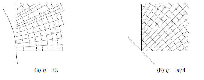
where we have used the abbreviations Uη=1+kcos⁡η​uU_{\eta}=\frac{\sqrt{1+k}}{\cos\eta}u, Vη=1−ksin⁡η​vV_{\eta}=\frac{\sqrt{1-k}}{\sin\eta}v and have written SηS_{\eta} for SS to emphasize the role of the parameter η\eta. As depicted in Figure 1, the distance function SηS_{\eta} is not the distance to any locus within the polytope, but to a virtual locus Sη=0S_{\eta}=0 in the u,vu,v plane that intersects the polytope only at (0,0)(0,0). See Figure 1.

Figure 1. Contour plots of the distance function SηS_{\eta} for two values of η\eta. Solid curve is the virtual locus Sη=0S_{\eta}=0, which touches the polytope only at (0,0)(0,0). Dashed curves are additional level-sets. Thin solid curves are characteristics for SηS_{\eta}, which are geodesics. Exactly one characteristic intersects the origin for each η\eta. We have chosen chirality number k=0.5k=0.5.
Refer to caption

3.2.2. The geodesics based at the origin

Because the virtual locus Sη=0S_{\eta}=0 intersects the polytope only at the origin, it follows that each choice of η\eta allows us to find a single geodesic from the origin. To study these geodesics from the origin, we attempt to solve for characteristics γ˙=∇Sη\dot{\gamma}=\nabla{}S_{\eta} with initial condition γ⁡(0,0)=(0,0)\gamma(0,0)=(0,0). For the gradient of SηS_{\eta} we have

(3.7) ∇Sη=2M​(cos2⁡η+(1+k)​u21+(1+k)​u2+(1−k)​v2​∂∂uCLOSEOPEN+sin2⁡η+(1−k)​v21+(1+k)​u2+(1−k)​v2​∂∂v).\displaystyle\begin{aligned} \nabla{S}_{\eta}&\;=\;\sqrt{\frac{2}{M}}\left(\frac{\sqrt{\cos^{2}\eta+(1+k)u^{2}}}{1+(1+k)u^{2}+(1-k)v^{2}}\frac{\partial}{\partial{u}}\right.\\ &\quad\quad\quad\quad\quad\quad\left.+\frac{\sqrt{\sin^{2}\eta+(1-k)v^{2}}}{1+(1+k)u^{2}+(1-k)v^{2}}\frac{\partial}{\partial{v}}\right).\end{aligned}

With γ⁡(t)=(u⁡(t),v⁡(t))\gamma(t)=(u(t),v(t)), the characteristic equation is the coupled autonomous system

(3.8) d​ud​t=cos2⁡η+(1+k)​u21+(1+k)​u2+(1−k)​v2,d​vd​t=sin2⁡η+(1+k)​v21+(1+k)​u2+(1−k)​v2.\displaystyle\begin{aligned} \quad\frac{du}{dt}&=\frac{\sqrt{\cos^{2}\eta+(1+k)u^{2}}}{1+(1+k)u^{2}+(1-k)v^{2}},\;\frac{dv}{dt}=\frac{\sqrt{\sin^{2}\eta+(1+k)v^{2}}}{1+(1+k)u^{2}+(1-k)v^{2}}.\end{aligned}

This is difficult to solve, but eliminating tt gives

(3.9) d​vd​u=sin2⁡η+(1−k)​v2cos2⁡η+(1+k)​u2,\displaystyle\frac{dv}{du}\;=\;\frac{\sqrt{\sin^{2}\eta+(1-k)v^{2}}}{\sqrt{\cos^{2}\eta+(1+k)u^{2}}},

which separates. At the point (u,v)=(0,0)(u,v)=(0,0) we see d​vd​u=tan⁡η\frac{dv}{du}=\tan\eta, which gives η\eta its geometric meaning: it is the initial angle the geodesic makes with the uu-axis. The solution for initial condition γ⁡(0)=(0,0)\gamma(0)=(0,0) is given explicitly by

(3.10) (Vη+1+Vη2)11−k=(Uη+1+Uη2)11+k\displaystyle\left(V_{\eta}\,+\,\sqrt{1+V_{\eta}{}^{2}}\right)^{\frac{1}{\sqrt{1-k}}}\;=\;\left(U_{\eta}\,+\,\sqrt{1+U_{\eta}{}^{2}}\right)^{\frac{1}{\sqrt{1+k}}}

and again Uη=1+k​ucos⁡ηU_{\eta}=\frac{\sqrt{1+k}\,u}{\cos\eta}, Vη=1−k​vsin⁡ηV_{\eta}=\frac{\sqrt{1-k}\,v}{\sin\eta}. This is the unparameterized geodesic equation.

3.2.3. Geodesic Normal Coordinates

Let R=dist(o,⋅)R=\mathop{\rm dist}(o,\cdot) be the distance function to the origin. If (u,v)(u,v) is an arbitrary point in the first quadrant, we wish to find both the distance R⁡(u,v)R(u,v) to the point and the initial angle η⁡(u,v)\eta(u,v) of the geodesic to that point. We find the initial angle of the geodesic through a given (u,v)(u,v) by solving the unparameterized geodesic equation (3.10) for η\eta:

(3.11) (v​1−ksin⁡η+1+(v​1−ksin⁡η)2)11−k=(u​1+kcos⁡η+1+(u​1+kcos⁡η)2)11+k.\displaystyle\begin{aligned} &\left(\frac{v\sqrt{1-k}}{\sin\eta}+\sqrt{1+\left(\frac{v\sqrt{1-k}}{\sin\eta}\right)^{2}}\right)^{\frac{1}{\sqrt{1-k}}}\\ &\quad\quad\quad\quad=\left(\frac{u\sqrt{1+k}}{\cos\eta}+\sqrt{1+\left(\frac{u\sqrt{1+k}}{\cos\eta}\right)^{2}}\right)^{\frac{1}{\sqrt{1+k}}}.\end{aligned}

This is a non-constructive step. Given uu, vv there is a unique solution η∈[0,π/2]\eta\in[0,\pi/2]. This is because when η\eta varies in [0,π/2][0,\pi/2] with uu and vv fixed, the left-hand side monotonically decreases from ∞\infty and the right-hand side monotonically increases to ∞\infty. Having found η=η⁡(u,v)\eta=\eta(u,v) this way, the distance to (u,v)(u,v) is now easy to determine:

(3.12) R⁡(u,v)=Sη⁡(u,v)​(u,v).\displaystyle R(u,v)\;=\;S_{\eta(u,v)}(u,\,v).

Thus we have described the transition from the isothermal system (u,v)(u,v) to polar geodesic coordinates (R,η)(R,\eta). This transformation is depicted in Figure 2.
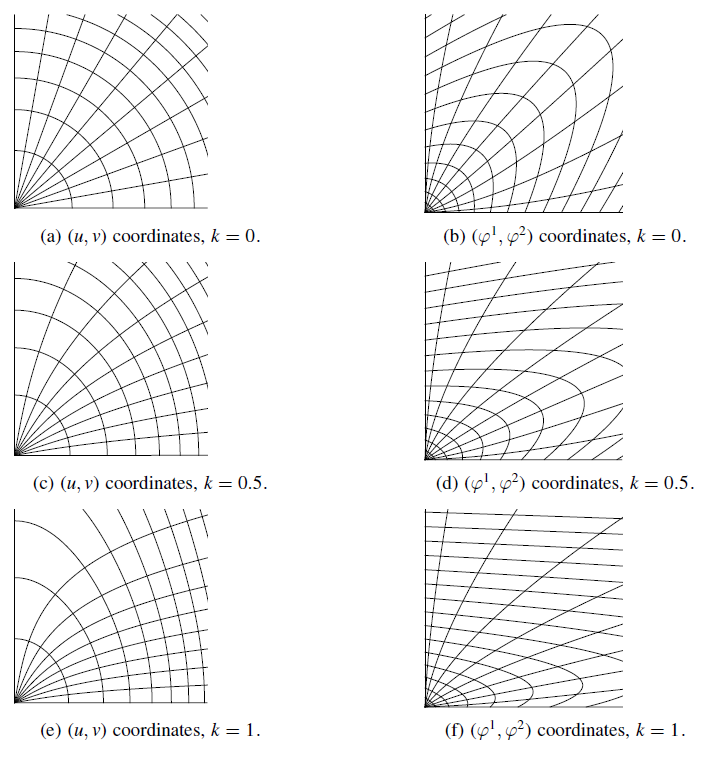
Figure 2. Depictions of geodesic polar coordinates in quadratic normal coordinates and in momentum coordinates. Shown are radial geodesics from the origin, and evenly spaced level-sets of the distance function.
Refer to caption

We must also compute the reverse transformation: given initial angle η\eta and distance RR, we must find (u,v)(u,v). This is equivalent to finding the parametrization for the geodesics described by (3.10). Given (R,η)(R,\eta) we must solve the non-algebraic system

(3.13) (Uη+1+Uη2)11+k=(Vη+1+Vη2)11−k,Sη​(u,v)=R\displaystyle\left(U_{\eta}+\sqrt{1+U_{\eta}{}^{2}}\right)^{\frac{1}{\sqrt{1+k}}}=\left(V_{\eta}+\sqrt{1+V_{\eta}{}^{2}}\right)^{\frac{1}{\sqrt{1-k}}},\;S_{\eta}(u,v)=R

for (u,v)(u,v). To do so, we define an auxiliary function FF by

(3.14) F≜(Uη+1+Uη2)11+k=(Vη+1+Vη2)11−k\displaystyle F\;\triangleq\;\left(U_{\eta}+\sqrt{1+U_{\eta}^{2}}\right)^{\frac{1}{\sqrt{1+k}}}\;=\;\left(V_{\eta}+\sqrt{1+V_{\eta}^{2}}\right)^{\frac{1}{\sqrt{1-k}}}

so that from FF we may determine uu and vv:

(3.15) u⁡(F)=cos⁡η2​1+k​(F1+k−F−1+k),v⁡(F)=sin⁡η2​1−k​(F1−k−F−1−k).\displaystyle\begin{aligned} &u(F)\;=\;\frac{\cos\eta}{2\sqrt{1+k}}\left(F^{\sqrt{1+k}}-F^{-\sqrt{1+k}}\right),\\ &v(F)\;=\;\frac{\sin\eta}{2\sqrt{1-k}}\left(F^{\sqrt{1-k}}-F^{-\sqrt{1-k}}\right).\end{aligned}

Using (3.6) we find that R=Sη​(u,v)R=S_{\eta}(u,v) is precisely

(3.16) R=2M​cos2⁡η2​1+k​[14​(F2​1+k−F−2​1+k)+log⁡F1+k]+2M​sin2⁡η2​1−k​[14​(F2​1−k−F−2​1−k)+log⁡F1−k].\displaystyle\begin{aligned} &R\;=\;\sqrt{\frac{2}{M}}\frac{\cos^{2}\eta}{2\sqrt{1+k}}\left[\frac{1}{4}\left(F^{2\sqrt{1+k}}-F^{-2\sqrt{1+k}}\right)+\log{F}^{\sqrt{1+k}}\right]\\ &\quad\quad+\sqrt{\frac{2}{M}}\frac{\sin^{2}\eta}{2\sqrt{1-k}}\left[\frac{1}{4}\left(F^{2\sqrt{1-k}}-F^{-2\sqrt{1-k}}\right)+\log{F}^{\sqrt{1-k}}\right].\end{aligned}

One then inverts this to obtain FF in terms of RR and η\eta, clearly a non-constructive step. To see that a solution exists and is unique for any choice of η\eta and RR, note that the right-hand side of (3.16), regarded as a function of FF, is monotone and has range (−∞,∞)(-\infty,\infty) as FF varies in (0,∞)(0,\infty). After finding F=F⁡(R,η)F=F(R,\eta) in this way, (3.15) gives u=u⁡(R,η)u=u(R,\eta) and v=v⁡(R,η)v=v(R,\eta).

In Section 3.2.4 we find simple, explicit expressions that approximate uu, vv, and FF as functions of RR and η\eta with good accuracy.

The coordinates (R,η)(R,\eta) are, of course, geodesic normal coordinates centered at (0,0)(0,0). To compute the metric in this system, consider again the unparameterized geodesic equation (3.11), which relates η\eta, uu, and vv. Taking an exterior derivative gives

(3.17) d​u+u​tan⁡η​d​ηcos2⁡η+(1+k)​u2=d​v−v​cot⁡η​d​ηsin2⁡η+(1−k)​v2.\displaystyle\frac{du\,+\,u\tan\eta\,d\eta}{\sqrt{\cos^{2}\eta+(1+k)u^{2}}}\;=\;\frac{dv\,-\,v\cot\eta\,d\eta}{\sqrt{\sin^{2}\eta+(1-k)v^{2}}}.

Since we have |d​u|2=|d​v|2=M2​(1+(1+k)​u2+(1−k)​v2)−1|du|^{2}=|dv|^{2}=\frac{M}{2}(1+(1+k)u^{2}+(1-k)v^{2})^{-1} and ⟨d​u,d​v⟩=0\left<du,dv\right>=0, we can isolate d​ηd\eta and norm to obtain

(3.18) |d​η|2​2M​(u​tan⁡η​sin2⁡η+(1−k)​v2+v​cot⁡η​cos2⁡η+(1+k)​u2)2=1.\displaystyle\quad|d\eta|^{2}\frac{2}{M}\left(u\tan\eta\sqrt{\sin^{2}\eta+(1-k)v^{2}}+v\cot\eta\sqrt{\cos^{2}\eta+(1+k)u^{2}}\right)^{2}=1.

Using (3.15) to write |d​η|2|d\eta|^{2} in terms of RR and η\eta, we obtain, finally, the polytope metric in geodesic normal coordinates:

(3.19) gΣ=d​R⊗d​R+A​(R,η)2​d​η⊗d​η,whereA​(R,η)2=|d​η|−2=[sin2⁡η2​M​1+k(F1+k−F−1+k)(F1−k+F−1−k)+cos2⁡η2​M​1−k(F1+k+F−1+k)(F1−k−F−1−k)]2.\displaystyle\begin{aligned} &g_{\Sigma}\;=\;dR\otimes{d}R\,+\,A(R,\eta)^{2}d\eta\otimes{d}\eta,\quad\text{where}\\ &A(R,\eta)^{2}\;=\;|d\eta|^{-2}\\ &\quad\quad\quad\;\;=\;\left[\frac{\sin^{2}\eta}{2M\sqrt{1+k}}\left(F^{\sqrt{1+k}}-F^{-\sqrt{1+k}}\right)\left(F^{\sqrt{1-k}}+F^{-\sqrt{1-k}}\right)\right.\\ &\quad\quad\quad\quad+\left.\frac{\cos^{2}\eta}{2M\sqrt{1-k}}\left(F^{\sqrt{1+k}}+F^{-\sqrt{1+k}}\right)\left(F^{\sqrt{1-k}}-F^{-\sqrt{1-k}}\right)\right]^{2}.\end{aligned}

3.2.4. Asymptotic approximations of FF and RR

The coordinates (u,v)(u,v) and the auxiliary function FF are functions of the polar coordinates (R,η)(R,\eta). In this section we approximate uu, vv and FF using closed-form expressions. We may approximate the value of FF to within tolerable margins by

(3.20) F~​(R,η)={(8​1+kcos2⁡η​M2​R)12​1+k,0≤η<η0(8​1−ksin2⁡η​M2​R)12​1−k,η0≤η≤π2,η0=sin−1⁡((M2​R)1+k1−k−1(M2​R)1+k1−k−1+6​1+k(8​1−k)1+k1−k).\displaystyle\begin{aligned} &\widetilde{F}(R,\eta)=\begin{cases}\left(\frac{8\sqrt{1+k}}{\cos^{2}\eta}\sqrt{\frac{M}{2}}R\right)^{\frac{1}{2\sqrt{1+k}}},&0\leq\eta<\eta_{0}\\ \left(\frac{8\sqrt{1-k}}{\sin^{2}\eta}\sqrt{\frac{M}{2}}R\right)^{\frac{1}{2\sqrt{1-k}}},&\eta_{0}\;\leq\;\eta\;\leq\;\frac{\pi}{2},\end{cases}\\ &\eta_{0}\;=\;\sin^{-1}\left(\frac{\left(\sqrt{\frac{M}{2}}R\right)^{\sqrt{\frac{1+k}{1-k}}-1}}{\left(\sqrt{\frac{M}{2}}R\right)^{\sqrt{\frac{1+k}{1-k}}-1}+\frac{6\sqrt{1+k}}{(8\sqrt{1-k})^{\sqrt{\frac{1+k}{1-k}}}}}\right).\end{aligned}

where “tolerable margins” means the following.

Lemma 3.1.

Given any values FF, η\eta, define the function ℛ=ℛ⁡(F,η)\mathcal{R}=\mathcal{R}(F,\eta) by

(3.21) ℛ=cos2⁡η2​M​1+k​[14​(F2​1+k−F−2​1+k)+log⁡F1+k]+sin2⁡η2​M​1−k​[14​(F2​1−k−F−2​1−k)+log⁡F1−k].\displaystyle\begin{aligned} &\mathcal{R}\;=\;\frac{\cos^{2}\eta}{\sqrt{2M}\sqrt{1+k}}\left[\frac{1}{4}\left(F^{2\sqrt{1+k}}-F^{-2\sqrt{1+k}}\right)+\log{F}^{\sqrt{1+k}}\right]\\ &\quad\quad+\frac{\sin^{2}\eta}{\sqrt{2M}\sqrt{1-k}}\left[\frac{1}{4}\left(F^{2\sqrt{1-k}}-F^{-2\sqrt{1-k}}\right)+\log{F}^{\sqrt{1-k}}\right].\end{aligned}

If F=F⁡(R,η)F=F(R,\eta) is the auxiliary function of (3.16) then of course the distance function is exactly R=ℛ⁡(F,η)R=\mathcal{R}(F,\eta). Given any ϵ>0\epsilon>0, then for sufficiently large RR we have

(3.22) ℛ​(F~​(R,η),η)R=ℛ​(F~​(R,η),η)ℛ⁡(F⁡(R,η),η)∈[1, 2+ϵ]\displaystyle\frac{\mathcal{R}(\widetilde{F}(R,\eta),\,\eta)}{R}\;=\;\frac{\mathcal{R}(\widetilde{F}(R,\eta),\,\eta)}{\mathcal{R}(F(R,\eta),\eta)}\;\in\;\left[1,\,2+\epsilon\right]

for all η∈[0,π/2]\eta\in[0,\pi/2].

Proof. Apply the first derivative test in the parameter η\eta to learn that the minimum of 1R​ℛ​(F~​(R,η),η)\frac{1}{R}\mathcal{R}(\widetilde{F}(R,\eta),\,\eta) occurs at the endpoints η=0,π/2\eta=0,\pi/2, and that the maximum occurs at the discontinuity point, where the left and right limits are different. Then test these points to learn that the minimum is 11 and the maximum is a bit bigger than 22. ∎

In short, our approximation F~\widetilde{F} for FF gives the correct value of RR to within about a factor of 2. With electronic help, this estimate can be improved with very little use of processing power. Just a single application of Newton’s method—or Householder’s method, which is better adapted for this problem—will bring this estimate to within an arbitrarily close multiple of RR for large RR.

This estimate for FF is valuable in approximating the metric as given in (3.19), but for determining the key asymptotic ratios a direct approximation of RR is preferable. We create approximations for (R,η)(R,\eta) with new coordinates (R~,η~)(\widetilde{R},\widetilde{\eta}) that we call almost polar coordinates, given by

(3.23) R~=1+k2​M​u2+1−k2​M​v2,η~=tan−1⁡(1−k1+k4​vu)\displaystyle\widetilde{R}\;=\;\sqrt{\frac{1+k}{2M}}\,u^{2}+\sqrt{\frac{1-k}{2M}}\,v^{2},\quad\quad\widetilde{\eta}\;=\;\tan^{-1}\left(\sqrt[4]{\frac{1-k}{1+k}}\frac{v}{u}\right)

with inverse transitions

(3.24) u=2​M1+k4​R~​cos⁡η~,v=2​M1−k4​R~​sin⁡η~.\displaystyle u=\sqrt[4]{\frac{2M}{1+k}}\sqrt{\widetilde{R}}\cos\widetilde{\eta},\quad\quad v=\sqrt[4]{\frac{2M}{1-k}}\sqrt{\widetilde{R}}\sin\widetilde{\eta}.

We shall see that the distance function RR and the “almost distance function” R~\widetilde{R} are asymptotically very close together. Unfortunately the angle η\eta and the “almost angle” η~\widetilde{\eta} are not uniformly close together. The following estimate is the best we are able to manage for η~\widetilde{\eta}.

Lemma 3.2.

Assuming R~\widetilde{R} is sufficiently large compared to MM and k∈(0,1)k\in(0,1), then

(3.25) cos⁡η~cos⁡η≥min⁡{12,[(2​M​(1−k)4)1+k1−k1+k]​R~1+k1−k−1}sin⁡η~sin⁡η≥min⁡{12,[(2​M​(1+k)4)1−k1+k1−k]​R~1−k1+k−1}.\displaystyle\begin{aligned} &\frac{\cos\widetilde{\eta}}{\cos\eta}\;\geq\;\min\left\{\frac{1}{\sqrt{2}},\,\left[\frac{\left(\sqrt[4]{2M(1-k)}\right)^{\frac{\sqrt{1+k}}{\sqrt{1-k}}}}{\sqrt{1+k}}\right]\sqrt{\widetilde{R}}^{\frac{\sqrt{1+k}}{\sqrt{1-k}}-1}\right\}\\ &\frac{\sin\widetilde{\eta}}{\sin\eta}\;\geq\;\min\left\{\frac{1}{\sqrt{2}},\,\left[\frac{\left(\sqrt[4]{2M(1+k)}\right)^{\frac{\sqrt{1-k}}{\sqrt{1+k}}}}{\sqrt{1-k}}\right]\sqrt{\widetilde{R}}^{\frac{\sqrt{1-k}}{\sqrt{1+k}}-1}\right\}.\end{aligned}

Indeed it suffices that M⁡(1−k)​R~\sqrt{M(1-k)}\,\widetilde{R} be larger than either of

(3.26) 12​(121+k1−k−1)1−k1+k,12​(121−k1+k−1)1+k1−k.\displaystyle\frac{1}{2}\left(\frac{1}{2^{\sqrt{\frac{1+k}{1-k}}}-1}\right)^{\sqrt{\frac{1-k}{1+k}}},\quad\frac{1}{2}\left(\frac{1}{2^{\sqrt{\frac{1-k}{1+k}}}-1}\right)^{\sqrt{\frac{1+k}{1-k}}}.
Proof.

We start with the first inequality. If already cos⁡η~cos⁡η≥12\frac{\cos\widetilde{\eta}}{\cos\eta}\geq\frac{1}{\sqrt{2}} then the inequality holds immediately, so assume cos⁡η~cos⁡η<12\frac{\cos\widetilde{\eta}}{\cos\eta}<\frac{1}{\sqrt{2}}. Using sin2⁡η~=1−cos2⁡η~>1−12​cos2⁡η=12+12​sin2⁡η\sin^{2}\widetilde{\eta}=1-\cos^{2}\widetilde{\eta}>1-\frac{1}{2}\cos^{2}\eta=\frac{1}{2}+\frac{1}{2}\sin^{2}\eta we obtain sin2⁡η~sin2⁡η>12​1+sin2⁡ηsin2⁡η≥1\frac{\sin^{2}\widetilde{\eta}}{\sin^{2}\eta}>\frac{1}{2}\frac{1+\sin^{2}\eta}{\sin^{2}\eta}\geq 1. Referring to the abbreviations Uη=1+kcos⁡η​uU_{\eta}=\frac{\sqrt{1+k}}{\cos\eta}u and Vη=1−ksin⁡η​vV_{\eta}=\frac{\sqrt{1-k}}{\sin\eta}v, by using sin2⁡η~sin2⁡η>1\frac{\sin^{2}\widetilde{\eta}}{\sin^{2}\eta}>1 and (3.24) we see

(3.27) Vη=v​1−ksin⁡η≥2​M​(1−k)4​R~.\displaystyle V_{\eta}\;=\;\frac{v\sqrt{1-k}}{\sin\eta}\;\geq\;\sqrt[4]{2M(1-k)}\sqrt{\widetilde{R}}.

By (3.14) we express F=(Vη+1+Vη2)11−kF=\left(V_{\eta}+\sqrt{1+V_{\eta}^{2}}\right)^{\frac{1}{\sqrt{1-k}}}, and since Vη+1+Vη2>2​VηV_{\eta}+\sqrt{1+V_{\eta}^{2}}>2V_{\eta} we now have

(3.28) F=(Vη+1+Vη2)11−k>(2​2​M​(1−k)4​R~)11−k.\displaystyle F\;=\;\left(V_{\eta}+\sqrt{1+V_{\eta}^{2}}\right)^{\frac{1}{\sqrt{1-k}}}\;>\;\left(2\sqrt[4]{2M(1-k)}\sqrt{\widetilde{R}}\right)^{\frac{1}{\sqrt{1-k}}}.

As long as we assume 2​M​(1−k)4​R~\sqrt[4]{2M(1-k)}\sqrt{\widetilde{R}} is larger than either of the expressions in (3.26), then we can use this estimate for FF to obtain an estimate for uu. Using (3.15) to express uu in terms of FF, we obtain

(3.29) u​1+kcos⁡η=F1+k−F−1+k>(2​M​(1−k)4​R~)1+k1−k\displaystyle\begin{aligned} \frac{u\sqrt{1+k}}{\cos\eta}\;=\;F^{\sqrt{1+k}}-F^{-\sqrt{1+k}}\;>\;\left(\sqrt[4]{2M(1-k)}\sqrt{\widetilde{R}}\right)^{\frac{\sqrt{1+k}}{\sqrt{1-k}}}\end{aligned}

Finally using the fact that u=R~​cos⁡η~u=\widetilde{R}\cos\widetilde{\eta} gives the stated conclusion.

The second inequality proceeds identically, exchanging vv for uu and so on. ∎

Corollary 3.3 (Estimate for the almost distance function).

Assuming R~\widetilde{R} is sufficiently large (as given by (3.26)), we have

(3.30) R~<R<(1+ϵ⁡(R~))​R~\displaystyle\widetilde{R}\;<\;R\;<\;\left(1+\epsilon(\widetilde{R})\right)\widetilde{R}

where ϵ⁡(R~)→0\epsilon(\widetilde{R})\rightarrow 0 as R~→∞\widetilde{R}\rightarrow\infty.

Proof.

Substituting the transitions u=2​M1+k4​R~​cos⁡η~u=\sqrt[4]{\frac{2M}{1+k}}\sqrt{\tilde{R}}\cos\widetilde{\eta}, v=2​M1−k4​R~​sin⁡η~v=\sqrt[4]{\frac{2M}{1-k}}\sqrt{\tilde{R}}\sin\widetilde{\eta} in the expression R=Sη⁡(u,v)​(u,v)R=S_{\eta(u,v)}(u,v) from (3.6), we obtain

R=R~​cos2⁡(η~)​1+cos2⁡η(1+k)​R~​cos2⁡η~+R~​sin2⁡(η~)​1+sin2⁡η(1−k)​R~​sin2⁡η~+cos2⁡η2​M​(1+k)​log⁡[2​M​(1+k)4​R~​cos⁡η~cos⁡η​(1+cos2⁡η1+k​R~​cos2⁡η~+1)]+sin2⁡η2​M​(1−k)​log⁡[2​M​(1−k)4​R~​sin⁡η~sin⁡η​(1+sin2⁡η1−k​R~​sin2⁡η~+1)].\displaystyle\begin{aligned} &R\;=\;\widetilde{R}\cos^{2}(\widetilde{\eta})\sqrt{1+\frac{\cos^{2}\eta}{(1+k)\widetilde{R}\cos^{2}\widetilde{\eta}}}+\widetilde{R}\sin^{2}(\widetilde{\eta})\sqrt{1+\frac{\sin^{2}\eta}{(1-k)\widetilde{R}\sin^{2}\widetilde{\eta}}}\\ &\quad\quad+\frac{\cos^{2}\eta}{\sqrt{2M(1+k)}}\log\left[\sqrt[4]{2M(1+k)}\frac{\sqrt{\widetilde{R}}\cos\widetilde{\eta}}{\cos\eta}\left(1+\sqrt{\frac{\cos^{2}\eta}{\sqrt{1+k}\widetilde{R}\cos^{2}\widetilde{\eta}}+1}\;\right)\right]\\ &\quad\quad+\frac{\sin^{2}\eta}{\sqrt{2M(1-k)}}\log\left[\sqrt[4]{2M(1-k)}\frac{\sqrt{\widetilde{R}}\sin\widetilde{\eta}}{\sin\eta}\left(1+\sqrt{\frac{\sin^{2}\eta}{\sqrt{1-k}\widetilde{R}\sin^{2}\widetilde{\eta}}+1}\;\right)\right].\end{aligned}

By Lemma 3.2 the values R~​cos2⁡η~cos2⁡η\frac{\sqrt{\widetilde{R}}\cos^{2}\widetilde{\eta}}{\cos^{2}\eta} and R~​sin2⁡η~sin2⁡η\frac{\sqrt{\widetilde{R}}\sin^{2}\widetilde{\eta}}{\sin^{2}\eta} both grow like a positive power of R~\widetilde{R}, namely like R~1+k1−k\sqrt{\widetilde{R}}{}^{\frac{\sqrt{1+k}}{\sqrt{1-k}}} or R~1−k1+k\sqrt{\widetilde{R}}{}^{\frac{\sqrt{1-k}}{\sqrt{1+k}}}, respectively. Consequently both logarithms are positive, and so we obtain R~<R\widetilde{R}<R.

For the upper bound on RR, using Lemma 3.2 again, we see cos2⁡ηR~​cos2⁡η~\frac{\cos^{2}\eta}{\sqrt{\widetilde{R}}\cos^{2}\widetilde{\eta}} and sin2⁡ηR~​sin2⁡η~\frac{\sin^{2}\eta}{\sqrt{\widetilde{R}}\sin^{2}\widetilde{\eta}} decay like a power of R~\widetilde{R}; this means the coefficients on R~​cos2⁡(η~)\tilde{R}\cos^{2}(\widetilde{\eta}) and R~​cos2⁡(η~)\tilde{R}\cos^{2}(\widetilde{\eta}) both approach 1. An easy estimate shows the logarithm terms are bounded from above by a definite multiple of R~​log⁡R~\sqrt{\tilde{R}}\log\widetilde{R}. Thus we conclude

(3.31) 1<RR~≤ 1+ϵ⁡(R~).\displaystyle 1\;<\;\frac{R}{\;\widetilde{R}\;}\;\leq\;1+\epsilon(\widetilde{R}).

∎

3.3. Computation of the asymptotic quantities

We make use of the “almost polar coordinates” (R~,η~)(\widetilde{R},\widetilde{\eta}) to compute the key asymptotic ratios of the generalized Taub-NUT instantons. We note that this section works only for the generalized Taub-NUT metrics because the almost polar coordinates in the two exceptional cases are not given by (3.23). The computations for the two exceptional instantons are deferred to Sections 5 and 6, respectively.

Before computing volumes, we must say a word about the ranges of the coordinates. Certainly R~∈[0,∞)\widetilde{R}\in[0,\infty), η~∈[0,π/2]\widetilde{\eta}\in[0,\pi/2]. But the ranges of θ1\theta_{1}, θ2\theta_{2} are somewhat peculiar:

(3.32) θ1,θ2∈[0,8​π).\displaystyle\theta_{1},\theta_{2}\in[0,\sqrt{8}\pi).

The ranges for θ1\theta_{1}, θ2\theta_{2} must be determined through understanding the Delzant gluing construction, where the requirement is that, near the polytope edges, the tori close up to create smooth manifolds without conical singularities. We examine the situation near a boundary point (u,0)(u,0) on the vv-axis. Consider the 2-manifold determined by fixing uu and θ2\theta_{2}, and varying the coordinates vv and θ1\theta_{1}. On this submanifold, the 4-manifold metric (3.3) restricts to

(3.33) g=[2M(1+(1+k)u2+(1−k)v2)(dv)2+1Mv2​((1+(1+k)​u2)2+(1+k)2​u2​v2)1+(1+k)​u2+(1−k)​v2(dθ1)2]\displaystyle\begin{aligned} g&\;=\;\left[\frac{2}{M}\left(1+(1+k)u^{2}+(1-k)v^{2}\right)(dv)^{2}\right.\\ &\quad\quad\left.+\frac{1}{M}\frac{v^{2}\left(\left(1+(1+k)u^{2}\right)^{2}+(1+k)^{2}u^{2}v^{2}\right)}{1+(1+k)u^{2}+(1-k)v^{2}}\,(d\theta_{1})^{2}\right]\\ \end{aligned}

for fixed uu. Using “big-OO” notation, we write this as

(3.34) g=2​(1+(1+k)​u2)M​[(1+O⁡(v2))​(d​v)2+12​v2​(1+O⁡(v2))​(d​θ1)2]=2​(1+(1+k)​u2)M​[(1+O⁡(v2))​(d​v)2+v2​(1+O⁡(v2))​(d​θ12)2].\displaystyle\begin{aligned} \quad\quad g&\;=\;\frac{2(1+(1+k)u^{2})}{M}\left[\left(1+O(v^{2})\right)(dv)^{2}\,+\,\frac{1}{2}v^{2}(1+O(v^{2}))\,(d\theta_{1})^{2}\right]\\ &\;=\;\frac{2(1+(1+k)u^{2})}{M}\left[\left(1+O(v^{2})\right)(dv)^{2}\,+\,v^{2}(1+O(v^{2}))\,\left(d\frac{\theta_{1}}{\sqrt{2}}\right)^{2}\right].\end{aligned}

Thus, for the central point (v,θ1)=(0,0)(v,\theta_{1})=(0,0) to be a smooth point rather than a cone point, the variable θ1/2\theta_{1}/\sqrt{2} must have range along the circle [0,2​π)[0,2\pi), meaning θ1\theta_{1} ranges along [0,8​π)[0,\sqrt{8}\pi). A similar argument works for the parameterization of θ2\theta_{2}.

The ball B⁡(S)B(S) of radius SS about the origin is the set of points with radius R<SR<S. Likewise let the almost ball A​B​(S)AB(S) of radius SS be

(3.35) A​B​(S)={(R~,η~,θ1,θ2)∈N4|R~<S}.\displaystyle AB(S)\;=\;\left\{\,(\widetilde{R},\widetilde{\eta},\theta_{1},\theta_{2})\in{}N^{4}\;\;\Big|\;\;\widetilde{R}\,<\,S\;\right\}.

By Lemma (3.3), we have A​B​(S)⊂B⁡(S)⊂A​B​(S⁡(1+ϵ))AB(S)\subset{B}(S)\subset{AB}(S(1+\epsilon)), where limS→∞ϵ=0\lim_{S\rightarrow\infty}\epsilon=0, and therefore V​o​l​B​(S)<V​o​l​A​B​(S)<V​o​l​B​(S⁡(1+ϵ))Vol\,B(S)\;<\;Vol\,AB(S)\;<\;Vol\,B(S(1+\epsilon)).

Proposition 3.4.

If k∈(−1,1)k\in(-1,1), then asymptotic volume growth of balls is cubic:

(3.36) limR→∞R−3​VolB⁡(R)=83​π2​12​M​(11−k+11+k).\displaystyle\lim_{R\rightarrow\infty}R^{-3}\,\mathop{\rm Vol}\,B(R)\;=\;\frac{8}{3}\pi^{2}\frac{1}{\sqrt{2M}}\,\left(\frac{1}{\sqrt{1-k}}+\frac{1}{\sqrt{1+k}}\right).
Proof.

In u,v,θ1,θ2u,v,\theta_{1},\theta_{2} coordinates, we can use (3.3) to compute the volume form:

(3.37) d​V​o​l=2M2​u​v​(1+(1+k)​u2+(1−k)​v2)​d​u∧d​v∧d​θ1∧d​θ2.\displaystyle\begin{aligned} &\quad{}dVol=\frac{2}{M^{2}}uv\left(1+(1+k)u^{2}+(1-k)v^{2}\right)\,du\wedge{d}v\wedge{d}\theta_{1}\wedge{d}\theta_{2}.\end{aligned}

Transitioning to almost polar coordinates we obtain

(3.38) d​V​o​l=2M​(1+2​M​(1+k)​R~​cos2⁡η~+2​M​(1−k)​R~​sin2⁡η~)⋅R~​cos⁡η~​sin⁡η~1−k2​d​R~∧d​η~∧d​θ1∧d​θ2.\displaystyle\begin{aligned} &dVol\;=\;\frac{2}{M}\left(1+\sqrt{2M(1+k)}\tilde{R}\cos^{2}\widetilde{\eta}+\sqrt{2M(1-k)}\tilde{R}\sin^{2}\widetilde{\eta}\right)\\ &\quad\quad\quad\quad\quad\quad\quad\quad\quad\quad\cdot\frac{\tilde{R}\cos\widetilde{\eta}\sin\widetilde{\eta}}{\sqrt{1-k^{2}}}\,d\tilde{R}\wedge{d}\widetilde{\eta}\wedge{d}\theta_{1}\wedge{d}\theta_{2}.\end{aligned}

The ranges for the coordinates are η~∈[0,π/2)\widetilde{\eta}\in[0,\pi/2) and θ1,θ2∈[0,8​π)\theta_{1},\theta_{2}\in[0,\sqrt{8}\pi). Integrating along these ranges and integrating R~\tilde{R} from 00 to SS gives

(3.39) VolA​B​(S)=83​π2​S32​M​1−k2​[3​S−1+(2​M​(1+k)+2​M​(1−k))].\displaystyle\mathop{\rm Vol}\,AB(S)=\frac{\frac{8}{3}\pi^{2}S^{3}}{2M\sqrt{1-k^{2}}}\left[3S^{-1}+\left(\sqrt{2M(1+k)}+\sqrt{2M(1-k)}\right)\right].

Using Lemma 3.3 to approximate balls with almost-balls, we have

(3.40) VolB⁡(S)≤83​π2​S32​M​1−k2​[3​S−1+(2​M​(1+k)+2​M​(1−k))]≤VolB⁡(S⁡(1+ϵ⁡(S))).\displaystyle\begin{aligned} \mathop{\rm Vol}\,B(S)&\leq\frac{\frac{8}{3}\pi^{2}S^{3}}{2M\sqrt{1-k^{2}}}\left[3S^{-1}+\left(\sqrt{2M(1+k)}+\sqrt{2M(1-k)}\right)\right]\quad\\ &\leq\mathop{\rm Vol}\,B(S(1+\epsilon(S))).\end{aligned}

so we see that volume growth is indeed cubic when k∈(−1,1)k\in(-1,1). Taking the limit,

(3.41) limS→∞S−3​VolB⁡(S)=83​π2​2​M​(1+k)+2​M​(1−k)2​M​1−k2.\displaystyle\begin{aligned} &\lim_{S\rightarrow\infty}S^{-3}\mathop{\rm Vol}\,B(S)\;=\;\frac{8}{3}\pi^{2}\;\frac{\sqrt{2M(1+k)}+\sqrt{2M(1-k)}}{2M\sqrt{1-k^{2}}}.\end{aligned}

∎

Lemma 3.5.

If KΣK_{\Sigma} is the polytope sectional curvature and k≠0,±1k\neq 0,\pm 1, then KΣ=O⁡(R−2)K_{\Sigma}=O(R^{-2}), except along a single path where KΣ=O⁡(R−3)K_{\Sigma}=O(R^{-3}). In almost polar coordinates,

(3.42) limR~→∞R~2​KΣ=k2​1+k​cos2⁡η~−1−k​sin2⁡η~(1+k​cos2⁡η~+1−k​sin2⁡η~)3.\displaystyle\lim_{\widetilde{R}\rightarrow\infty}\widetilde{R}^{2}{}K_{\Sigma}\;=\;\frac{k}{2}\frac{\sqrt{1+k}\cos^{2}\widetilde{\eta}-\sqrt{1-k}\sin^{2}\widetilde{\eta}}{\left(\sqrt{1+k}\cos^{2}\widetilde{\eta}+\sqrt{1-k}\sin^{2}\widetilde{\eta}\right)^{3}}.

If k=0k=0 then KΣ=O⁡(R−3)K_{\Sigma}=O(R^{-3}) along all paths to infinity.

Proof.

Using the expression (3.2) and the transitions to R~\widetilde{R}, η~\widetilde{\eta} we obtain

(3.43) KΣ=M​−1+k​2​M​R~​(1+k​cos2⁡η~−1−k​sin2⁡η~)(1+2​M​(1+k)​R~​cos2⁡η~+2​M​(1−k)​R~​sin2⁡η~)3=k2​1R~2​−1k​2​M​R~+1+k​cos2⁡η~−1−k​sin2⁡η~(12​M​R~+1+k​cos2⁡η~+1−k​sin2⁡η~)3.\displaystyle\begin{aligned} K_{\Sigma}&\;=\;M\,\frac{-1+k\sqrt{2M}\,\widetilde{R}\left(\sqrt{1+k}\cos^{2}\widetilde{\eta}-\sqrt{1-k}\sin^{2}\widetilde{\eta}\right)}{\left(1+\sqrt{2M(1+k)}\,\widetilde{R}\cos^{2}\widetilde{\eta}+\sqrt{2M(1-k)}\,\widetilde{R}\sin^{2}\widetilde{\eta}\right)^{3}}\\ &\;=\;\frac{k}{2}\frac{1}{{\widetilde{R}}^{2}}\,\frac{-\frac{1}{k\sqrt{2M}\widetilde{R}}+\sqrt{1+k}\cos^{2}\widetilde{\eta}-\sqrt{1-k}\sin^{2}\widetilde{\eta}}{\left(\frac{1}{\sqrt{2M}\widetilde{R}}+\sqrt{1+k}\,\cos^{2}\widetilde{\eta}+\sqrt{1-k}\,\sin^{2}\widetilde{\eta}\right)^{3}}.\end{aligned}

Taking a limit, then, we obtain

(3.44) limR~→∞R~2​KΣ=k2​1+k​cos2⁡η~−1−k​sin2⁡η~(1+k​cos2⁡η~+1−k​sin2⁡η~)3\displaystyle\lim_{\widetilde{R}\rightarrow\infty}\widetilde{R}^{2}K_{\Sigma}\;=\;\frac{k}{2}\frac{\sqrt{1+k}\cos^{2}\widetilde{\eta}-\sqrt{1-k}\sin^{2}\widetilde{\eta}}{\left(\sqrt{1+k}\cos^{2}\widetilde{\eta}+\sqrt{1-k}\sin^{2}\widetilde{\eta}\right)^{3}}

Therefore KΣ=O⁡(R~−2)=O⁡(R−2)K_{\Sigma}=O(\tilde{R}^{-2})=O(R^{-2}) except along a single path which is the path of constant η~\widetilde{\eta} where sin⁡η~cos⁡η~=1+k4/1−k4\frac{\sin\tilde{\eta}}{\cos\tilde{\eta}}=\sqrt[4]{1+k}/\sqrt[4]{1-k}.

When k=0k=0 then (3.43) gives KΣ=O⁡(R−3)K_{\Sigma}=O(R^{-3}) everywhere. ∎

Lemma 3.6.

Let (Σ2,gΣ)(\Sigma^{2},g_{\Sigma}) be a Taub-NUT polytope with k∈[−1,1]k\in[-1,1]. The Ricci potentials are

(3.45) ℛ1=12​1+(1+k)​(u2+v2)1+(1+k)​u2+(1−k)​v2,ℛ2=12​1+(1−k)​(u2+v2)1+(1+k)​u2+(1−k)​v2,\displaystyle\begin{aligned} &\mathcal{R}^{1}\;=\;\frac{1}{\sqrt{2}}\frac{1+(1+k)(u^{2}+v^{2})}{1+(1+k)u^{2}+(1-k)v^{2}},\\ &\mathcal{R}^{2}\;=\;\frac{1}{\sqrt{2}}\frac{1+(1-k)(u^{2}+v^{2})}{1+(1+k)u^{2}+(1-k)v^{2}},\end{aligned}

the norm of Ricci curvature is

(3.46) |Ric|=4​|k|​M(1+(1+k)​u2+(1−k)​v2)2,\displaystyle\begin{aligned} |\mathop{\rm Ric}|&\;=\;\frac{4|k|M}{\left(1+(1+k)u^{2}+(1-k)v^{2}\right)^{2}},\end{aligned}

and we have

(3.47) |Ric|2dVol4=2​u​vM2(1+(1+k)u2+(1−k)v2)du∧dv∧dθ1∧dθ2.\displaystyle\quad\quad\quad|\mathop{\rm Ric}|^{2}dVol_{4}=\frac{2uv}{M^{2}}\left(1+(1+k)u^{2}+(1-k)v^{2}\right)du\wedge{}dv\wedge{}d\theta_{1}\wedge{}d\theta_{2}.
Proof.

From Section 2.3 the Ricci potentials are defined by ℛi=⟨∇φi,∇log⁡x⟩\mathcal{R}^{i}=\left<\nabla\varphi^{i},\,\nabla\log\mathcal{}x\right>; an elementary computation gives (3.45). Using (2.10), we compute |Ric|2dVol4|\mathop{\rm Ric}|^{2}dVol_{4}:

(3.48) |Ric|2dVol4= 4dℛ1∧dℛ2∧dθ1∧dθ2=32​k2​u​v(1+(1+k)​u2+(1−k)​v2)3​d​u∧d​v∧d​θ1∧d​θ2.\displaystyle\begin{aligned} &|\mathop{\rm Ric}|^{2}dVol_{4}\;=\;4\,d\mathcal{R}^{1}\wedge{}d\mathcal{R}^{2}\wedge{}d\theta_{1}\wedge{}d\theta_{2}\\ &\quad\;=\;\frac{32k^{2}uv}{\left(1+(1+k)u^{2}+(1-k)v^{2}\right)^{3}}\,du\wedge{}dv\wedge{}d\theta_{1}\wedge{}d\theta_{2}.\end{aligned}

Using (3.3) we compute d​V​o​l4dVol_{4} in (u,v,θ1,θ2)(u,v,\theta_{1},\theta_{2}) coordinates:

(3.49) d​V​o​l4=2​u​vM2​(1+(1+k)​u2+(1−k)​v2)​d​u∧d​v∧d​θ1∧d​θ2\displaystyle dVol_{4}=\frac{2uv}{M^{2}}\left(1+(1+k)u^{2}+(1-k)v^{2}\right)\,du\wedge{}dv\wedge{}d\theta_{1}\wedge{}d\theta_{2}

so therefore

(3.50) |Ric|2=16​k2​M2(1+(1+k)​u2+(1−k)​v2)4.\displaystyle\begin{aligned} |\mathop{\rm Ric}|^{2}&\;=\;\frac{16k^{2}M^{2}}{\left(1+(1+k)u^{2}+(1-k)v^{2}\right)^{4}}.\end{aligned}

∎

Proposition 3.7 (Curvature Decay Rates).

In the generic case k≠0,±1k\neq 0,\pm 1, we have |Ric|,|W−|=O(R−2)|\mathop{\rm Ric}|,|W^{-}|=O(R^{-2}). In the case k=0k=0 we have |W−|=O⁡(R−3)|W^{-}|=O(R^{-3}).

Proof.

If W=W++W−W=W^{+}+W^{-} is the Weyl tensor, the computation of W−W^{-} from (A.46) and the fact that W+=0W^{+}=0 gives

(3.51) |W|2= 96​|KΣ|2\displaystyle|W|^{2}\;=\;96|K_{\Sigma}|^{2}

so from Lemma 3.5 we obtain the claimed R−2R^{-2} decay rate for |W−||W^{-}|. From Lemma 3.6

(3.52) |Ric|=4​|k|​M(1+(1+k)​u2+(1−k)​v2)2.\displaystyle|\mathop{\rm Ric}|\;=\;\frac{4|k|M}{\left(1+(1+k)u^{2}+(1-k)v^{2}\right)^{2}}.

Using Corollary 3.3 and changing to the almost polar coordinates, we obtain

(3.53) |Ric|=4​k​M(1+2​M​(1+k)​R~​cos2⁡η~+2​M​(1−k)​R~​sin2⁡η~)2.\displaystyle|\mathop{\rm Ric}|\;=\;\frac{4kM}{\left(1+\sqrt{2M(1+k)}\,\widetilde{R}\cos^{2}\widetilde{\eta}+\sqrt{2M(1-k)}\,\widetilde{R}\sin^{2}\widetilde{\eta}\right)^{2}}.

When kk is not 0,1,−10,1,-1 we see that |Ric|=O(R~−2)=O(R−2)|\mathop{\rm Ric}|=O(\tilde{R}^{-2})=O(R^{-2}). We now have that both |Ric||\mathop{\rm Ric}| and |W−||W^{-}| are O⁡(R−2)O(R^{-2}).

When k=0k=0 we have Ric=0\mathop{\rm Ric}=0 and therefore KΣ=O⁡(R−3)K_{\Sigma}=O(R^{-3}) gives |W−|=O⁡(R−3)|W^{-}|=O(R^{-3}). ∎

3.4. L2L^{2} norms

Using the “Ricci potentials” from section 2.3 and the computation of W−W^{-} from the appendix, we can compute the L2L^{2} norms of |Ric||\mathop{\rm Ric}| and |Rm||\mathop{\rm Rm}|.

To evaluate these integral norms on the 4-manifold parameterized by (u,v,θ1,θ2)(u,v,\theta_{1},\theta_{2}), we use the parameterization

(3.54) u,v∈[0,∞)andθ1,θ2∈[0,8​π)\displaystyle u,v\in[0,\infty)\quad\text{and}\quad\theta_{1},\theta_{2}\in[0,\sqrt{8}\pi)

discussed in Section 3.3.

Proposition 3.8.

The L2L^{2} norms of the Ricci and Riemann tensors are

(3.55) L2(Ric)= 32π2k21−k2,L2(W)= 32π21+k21−k2,L2​(Rm)= 32​π2​1+3​k21−k2.\displaystyle\begin{aligned} &L^{2}(\mathop{\rm Ric})\;=\;32\pi^{2}\frac{k^{2}}{1-k^{2}},\quad L^{2}(W)\;=\;32\pi^{2}\frac{1+k^{2}}{1-k^{2}},\\ &\quad\quad\quad\quad L^{2}(\mathop{\rm Rm})\;=\;32\pi^{2}\frac{1+3k^{2}}{1-k^{2}}.\end{aligned}
Proof.

In (3.48) we computed

(3.56) |Ric|2dVol4=32​k2​u​v(1+(1+k)​u2+(1−k)​v2)3​d​u∧d​v∧d​θ1∧d​θ2.\displaystyle\begin{aligned} &|\mathop{\rm Ric}|^{2}dVol_{4}\\ &\quad\quad\;=\;\frac{32k^{2}uv}{\left(1+(1+k)u^{2}+(1-k)v^{2}\right)^{3}}\,du\wedge{d}v\wedge{}d\theta_{1}\wedge{}d\theta_{2}.\end{aligned}

Integrating along θ1,θ2∈[0,8​π)\theta_{1},\theta_{2}\in[0,\sqrt{8}\pi), we have

(3.57) ∫N4|Ric|2dVol4= 8π2∫Σ232​k2​u​v(1+(1+k)​u2+(1−k)​v2)3du∧dv.\displaystyle\begin{aligned} &\quad\int_{N^{4}}|\mathop{\rm Ric}|^{2}dVol_{4}\;=\;8\pi^{2}\int_{\Sigma^{2}}\frac{32k^{2}uv}{\left(1+(1+k)u^{2}+(1-k)v^{2}\right)^{3}}\,du\wedge{d}v.\end{aligned}

Integrating uu, vv from 00 to ∞\infty gives

(3.58) ∫N4|Ric|2dVol4=32​π2​k21−k2.\displaystyle\begin{aligned} &\quad\int_{N^{4}}|\mathop{\rm Ric}|^{2}dVol_{4}\;=\;\frac{32\pi^{2}k^{2}}{1-k^{2}}.\end{aligned}

Using the computation |W−|2=96KΣ2|W^{-}|^{2}=96K_{\Sigma}{}^{2} of (A.46) and also using (3.2) and (3.3) to compute the volume form, we have

(3.59) |W−|2= 96​M2​(−1+k⁡((1+k)​u2−(1−k)​v2)(1+(1+k)​u2+(1−k)​v2)3)2andd​V​o​l4=2​u​vM2​(1+(1+k)​u2+(1−k)​v2)​d​u∧d​v∧d​θ1∧d​θ2\displaystyle\begin{aligned} &|W^{-}|^{2}\;=\;96M^{2}\left(\frac{-1+k\left((1+k)u^{2}-(1-k)v^{2}\right)}{\left(1+(1+k)u^{2}+(1-k)v^{2}\right)^{3}}\right)^{2}\quad\text{and}\\ &dVol_{4}=\frac{2uv}{M^{2}}\left(1+(1+k)u^{2}+(1-k)v^{2}\right)du\wedge{}dv\wedge{}d\theta_{1}\wedge{}d\theta_{2}\end{aligned}

Integrating θ1\theta_{1}, θ2\theta_{2} along [0,8​π)[0,\sqrt{8}\pi) and u,vu,v along [0,∞)[0,\infty) gives L2​(|W−|)=32​π2​1+k21−k2L^{2}(|W^{-}|)=32\pi^{2}\frac{1+k^{2}}{1-k^{2}}.

The value of ∫|Rm|2dVol4\int|\mathop{\rm Rm}|^{2}dVol_{4} follows from the identity |Rm|2=s26+2|Rı​∘ ​c|2+|W|2|\mathop{\rm Rm}|^{2}=\frac{s^{2}}{6}+2|\mathop{\rm R\char 16\relax\makebox[0.0pt]{\raisebox{5.0pt}{\tiny$\circ$\;\,}}c}|^{2}+|W|^{2} and the fact that our manifolds are scalar-flat and half-conformally flat. ∎

The Chern-Gauss-Bonnet formula for the Euler class is χ(N4)=18​π2∫R224−12|Rı​∘ ​c|2+14|W|2\chi(N^{4})=\frac{1}{8\pi^{2}}\int\frac{R^{2}}{24}-\frac{1}{2}|\mathop{\rm R\char 16\relax\makebox[0.0pt]{\raisebox{5.0pt}{\tiny$\circ$\;\,}}c}|^{2}+\frac{1}{4}|W|^{2}. In some presentations the factor of 14\frac{1}{4} on the |W|2|W|^{2} term is not present, which is due to norming WW as an operator ⋀2→⋀2\bigwedge^{2}\rightarrow\bigwedge^{2} instead of as a tensor; see the discussion after Lemma A.9 in the Appendix. Using the L2L^{2} norms of Proposition 3.8 we see immediately that χ⁡(N4)=1\chi(N^{4})=1, as expected.

We remark that the signature of these manifolds is zero, but ∫|W+|2−|W−|2≠0\int|W^{+}|^{2}-|W^{-}|^{2}\neq 0. As a result, Lemma 3.8 can be used to compute η\eta-invariants of various squashed 3-spheres. We do not pursue this further however.

4. Three kinds of Blowdown

The asymptotic geometry of open manifolds, including tangent cones at infinity and blowdown limits, are important in the study of open manifolds. Our investigation of the generalized Taub-NUTs ends with an examination of their blowdown objects, where we find some surprises.

Given a metric gg on a complete 44-manifold N4N^{4}, a Gromov-Hausdorff blowdown limit (colloquially known as a tangent cone at infinity) is a Gromov-Hausdorff limit of the manifold N4N^{4} with metric ϵi2​g\epsilon_{i}^{2}g as ϵi↘0\epsilon_{i}\searrow 0. In general such limits need not exist, and when they exist they need not be unique, and need not even be manifolds.

In this paper the objects have, for the most part, cubic volume growth and quadratic curvature decay |Rm|=O(r−2)|\mathop{\rm Rm}|=O(r^{-2}). Therefore we expect limits to exist, and by computation we find they are unique. The tangent cones at infinity are collapsed as expected, but they are not necessarily 3-dimensional as one might expect.

By (4.3) we see the polytope metric itself converges uniquely under blowdown, but the situation on the full instanton is more complex, as there is a complicating geometric issue. Level-sets of the distance function are spheres. The collapsing field foliates the Hopf tori on these spheres, and this field might be rational or irrational. Since 𝒳1\mathcal{X}^{1} and 𝒳2\mathcal{X}^{2} are the principle rotations on the level-sets and since the collapsing field is 𝒳=(1−k)​𝒳1−(1+k)​𝒳2\mathcal{X}=(1-k)\mathcal{X}^{1}-(1+k)\mathcal{X}^{2}, this Hopf foliation is rational if and only if kk is rational.

In the rational case, the spherical level-sets converge down to 𝕊2\mathbb{S}^{2} with up to two orbifold points, and in the irrational case the spherical level-sets converge down to a line segment (see Example 1.4 (continued) and Example 2.1 on pg 326 of [4]). Therefore when kk is rational the instanton blows down to a complete 3-dimensional stratified orbifold, and when kk is irrational it blows down to a 2-manifold with boundary.

Because this behavior is rather pathological, we choose to modify the usual blowdown process in order to obtain better behavior in the limits. The three kinds of blowdown are as follows. The first is the usual Gromov-Hausdorff blowdown of (N4,g)(N^{4},g) itself, which we have just described. The second and third kinds of blowdown, which we call “generalized blowdowns,” eliminate the pathologies arising from possibly irrational collapsing fields. The second kind of blowdown is performed by “unwrapping” the torus fibers—this is just taking the interior of the polytope crossed with ℝ2\mathbb{R}^{2} instead of with the torus, and simply declining to apply the Delzant gluing process on the boundary. So a new 4-manifold (not geodesically complete) exists with ℝ2\mathbb{R}^{2} fibers instead of torus fibers over each point of the polytope. Then we take the blowdown limit of this object. The metric has a zero eigen-direction on the ℝ2\mathbb{R}^{2} fibers. We throw this direction away so now we have an ℝ1\mathbb{R}^{1}-bundle over the polytope. Finally we compactify the line fibers into circle fibers and so obtain a stratified limiting 3-conifold. This conifold is an orbifold precisely when kk is rational.

For the third kind of “blowdown” limit, we take the blowdown on the polytope Σ2\Sigma^{2} itself without regarding it as part of a larger 4-manifold. This blowdown converges uniquely to a 2-manifold with boundary, and has a Riemannian metric with a curvature singularity at the origin. Still, it has two well-defined momentum functions, so we can artificially perform the Delzant construction and still produce an honest 4-dimensional manifold with a Riemannian metric that has a point-like curvature singularity.

4.1. Metric and coordinate convergence under blowdown

From (3.2) the polytope metric for the generalized Taub-NUTs is

(4.1) gΣ=2M​(1+(1+k)​u2+(1−k)​v2)​(d​u2+d​v2).\displaystyle g_{\Sigma}=\frac{2}{M}\left(1+(1+k)u^{2}+(1-k)v^{2}\right)\left(du^{2}+dv^{2}\right).

The 4-metric is g4=gΣ+Gi​j​d​θi⊗d​θjg_{4}=g_{\Sigma}+G^{ij}d\theta_{i}\otimes{d}\theta_{j} where Gi​jG^{ij} is the matrix from (3.3). Scaling the coordinates by setting u=M/24​u~u=\sqrt[4]{M/2}\,\tilde{u}, v=M/24​v~v=\sqrt[4]{M/2}\,\tilde{v}, the polytope metric becomes

(4.2) gΣ=(2M+(1+k)​u~2+(1−k)​v~2)​(d​u~2+d​v~2),\displaystyle\begin{aligned} g_{\Sigma}&=\left(\sqrt{\frac{2}{M}}+(1+k)\tilde{u}^{2}+(1-k)\tilde{v}^{2}\right)\left(d\tilde{u}^{2}+d\tilde{v}^{2}\right),\end{aligned}

and we can send M→∞M\rightarrow\infty. Both metrics gΣg_{\Sigma} and g4g_{4} converge. We get

(4.3) gΣ=((1+k)​u~2+(1−k)​v~2)​(d​u~2+d​v~2),Gi​j=12​u~2​v~2​(u~2+v~2)(1+k)​u~2+(1−k)​v~2​((1+k)21−k21−k2(1−k)2).\displaystyle\begin{aligned} &g_{\Sigma}=\left((1+k)\tilde{u}^{2}+(1-k)\tilde{v}^{2}\right)\left(d\tilde{u}^{2}+d\tilde{v}^{2}\right),\\ &G^{ij}\;=\;\frac{\frac{1}{2}\tilde{u}^{2}\tilde{v}^{2}(\tilde{u}^{2}+\tilde{v}^{2})}{(1+k)\tilde{u}^{2}+(1-k)\tilde{v}^{2}}\left(\begin{array}[]{cc}(1+k)^{2}&1-k^{2}\\ 1-k^{2}&(1-k)^{2}\end{array}\right).\end{aligned}

Note that det(Gi​j)=0\det(G^{ij})=0. Its zero eigenvector is v→=(1−k)​∂∂θ1−(1+k)​∂∂θ2\vec{v}=(1-k)\frac{\partial}{\partial\theta_{1}}-(1+k)\frac{\partial}{\partial\theta_{2}} and its eigenvector of eigenvalue u~​v~​(u~2+v~2)​((1+k)2+(1−k)2)4​((1+k)​u~2+(1−k)​v~2)\frac{\tilde{u}\tilde{v}(\tilde{u}^{2}+\tilde{v}^{2})((1+k)^{2}+(1-k)^{2})}{4((1+k)\tilde{u}^{2}+(1-k)\tilde{v}^{2})} is v→=(1+k)​∂∂θ1+(1−k)​∂∂θ2\vec{v}=(1+k)\frac{\partial}{\partial\theta_{1}}+(1-k)\frac{\partial}{\partial\theta_{2}}. Setting θ~=12​(1+k2)​((1+k)​θ1+(1−k)​θ2)\tilde{\theta}=\frac{1}{2(1+k^{2})}\left((1+k)\theta_{1}+(1-k)\theta_{2}\right) gives a 3-dimensional metric of

(4.4) g=((1+k)​u~2+(1−k)​v~2)​(d​u~2+d​v~2)+12​u~2​v~2​(u~2+v~2)(1+k)​u~2+(1−k)​v~2​(d​θ~)2.\displaystyle\begin{aligned} \quad&\quad\quad{}g=\left((1+k)\tilde{u}^{2}+(1-k)\tilde{v}^{2}\right)\left(d\tilde{u}^{2}+d\tilde{v}^{2}\right)+\frac{\frac{1}{2}\tilde{u}^{2}\tilde{v}^{2}(\tilde{u}^{2}+\tilde{v}^{2})}{(1+k)\tilde{u}^{2}+(1-k)\tilde{v}^{2}}(d{\tilde{\theta}})^{2}.\end{aligned}

The question of parameterization of θ~\tilde{\theta} can be determined as follows. The field ∂/∂θ~\partial/\partial\tilde{\theta} produces a subgroup of the torus of slope (1+k)/(1−k)(1+k)/(1-k). If k=m/nk=m/n is rational then this subgroup has slope m+n/m−nm+n/m-n, and so, for θ~\tilde{\theta} to obtain consistent values in the limit, it must have parameterization θ~∈[0,2​2​(1+k2)​π/L​C​M​(m+n,m−n))\tilde{\theta}\in[0,2\sqrt{2(1+k^{2})}\pi/LCM(m+n,m-n)). Certainly if kk becomes irrational then the parametrization vanishes and hence the Gromov-Hausdorff limit collapses to a 2-dimensional object with no θ~\tilde{\theta} variable.

In the limit the metric (4.4) no longer produces smooth points at the coordinate axes unless k=0k=0. Imitating the analysis at the beginning of Section 3.3 at the coordinate axes, we can fix a positive value of u~\tilde{u} and examine the 2-dimensional submanifold given by varying v~\tilde{v}, θ~\tilde{\theta}, to obtain the metric

(4.5) g=(1+k)u~2((1+O(v~2))dv~2+12​(1+k)2v~2(1+O(v~2)(dθ~)2).\displaystyle\begin{aligned} &\quad\quad{}g=(1+k)\tilde{u}^{2}\left(\left(1+O(\tilde{v}^{2})\right)d\tilde{v}^{2}+\frac{1}{2(1+k)^{2}}\tilde{v}^{2}(1+O(\tilde{v}^{2})(d{\tilde{\theta}})^{2}\right).\end{aligned}

and we can fix the value of u~\tilde{u} and examine the 2-dimensional submanifold given by varying u~\tilde{u}, θ~\tilde{\theta}, to obtain the metric

(4.6) g=(1−k)v~2((1+O(u~2))du~2+12​(1−k)2u~2(1+O(u~2)(dθ~)2).\displaystyle\begin{aligned} &\quad\quad{}g=(1-k)\tilde{v}^{2}\left(\left(1+O(\tilde{u}^{2})\right)d\tilde{u}^{2}+\frac{1}{2(1-k)^{2}}\tilde{u}^{2}(1+O(\tilde{u}^{2})(d{\tilde{\theta}})^{2}\right).\end{aligned}

When kk is rational we therefore observe a cone angle of 2​π​(1+k2)/(1+k)​L​C​M​(m+n,m−n)2\pi(1+k^{2})/(1+k)LCM(m+n,m-n) along the v~\tilde{v}-axis and a cone angle of2​π​(1+k2)/2​(1−k)​L​C​M​(m+n,m−n)2\pi(1+k^{2})/2(1-k)LCM(m+n,m-n) along the u~\tilde{u}-axis, These expressions are rational, so we observe a stratified orbifold in the limit.

When the collapsing field is irrational, the Gromov-Hausdorff limit does not produce such an object. Following the discussion in Example 1.4 (continued) and Example 2.1 on pg 326 of [4], when the collapsing direction is irrational it collapses the spheres to line segments.

The central observation of the first “generalized blowdown” is that the metric (4.4) makes sense on a 3-dimensional conifold, whether or not it is the result of a Gromov-Hausdorff blowdown. We simply declare (4.4) to be a metric on (u~,v~,θ~)(\tilde{u},\tilde{v},\tilde{\theta}) where u~,v~∈[0,∞)\tilde{u},\tilde{v}\in[0,\infty) and we give θ~\tilde{\theta} the range [0,8​π)[0,\sqrt{8}\pi) whether or not this is the range inherited from the Gromov-Hausdorff blowdown. Of course one may give θ~\tilde{\theta} any other range—this will affect the cone angles but can never make both cone angles equal to 2​π2\pi unless k=0k=0, so can never produce a smooth manifold for k≠0k\neq 0. In the irrational case, both cone angles (along the two axes) cannot be simultaneously made rational, so for irrational kk we can produce a variety of stratified conifolds depending on the parameterization chosen for θ~\tilde{\theta}, but we can never produce an orbifold.

We clearly still have a Killing field 𝒳~=∂/∂θ~\tilde{\mathcal{X}}={\partial}/{\partial\tilde{\theta}}, and we may take a Riemannian quotient along to obtain the quarter-plane polytope again. Its sectional curvature is

(4.7) KΣ=k​(1+k)​u~2−(1−k)​v~2((1+k)​u~2+(1−k)​v~2)3.\displaystyle K_{\Sigma}\;=\;k\frac{(1+k)\tilde{u}^{2}-(1-k)\tilde{v}^{2}}{\left((1+k)\tilde{u}^{2}+(1-k)\tilde{v}^{2}\right)^{3}}.

We see an irremovable curvature singularity at the origin (u~,v~)=(0,0)(\tilde{u},\tilde{v})=(0,0). It is also not difficult to compute the Ricci curvature of the conifold. It is diagonal in (u~,v~,θ~)(\tilde{u},\tilde{v},\tilde{\theta}) coordinates, and is given by

Ric=3(−4​k(1+k)​u~2+(1−k)​v~20004​k(1+k)​u~2+(1−k)​v~20002​k​(1+k)2​u~2​v~2​(u~2−v~2)((1+k)​u~2+(1−k)​v~2)3)\displaystyle\mathop{\rm Ric}{}_{3}=\left(\begin{array}[]{ccc}\frac{-4k}{(1+k)\tilde{u}^{2}+(1-k)\tilde{v}^{2}}&0&0\\ 0&\frac{4k}{(1+k)\tilde{u}^{2}+(1-k)\tilde{v}^{2}}&0\\ 0&0&\frac{2k(1+k)^{2}\tilde{u}^{2}\tilde{v}^{2}(\tilde{u}^{2}-\tilde{v}^{2})}{\left((1+k)\tilde{u}^{2}+(1-k)\tilde{v}^{2}\right)^{3}}\end{array}\right)

One notices immediately that scalar curvature is not zero.

4.2. The second generalized blowdown

The final type of “blowdown” comes out of the recognition that, in either of the two other blowdown processes, we always obtain a metric polytope, and that any such polytope does indeed encode all metric, complex structure, and curvature information for some scalar-flat 4-dimensional instanton, whether or not this 4-dimensional object has anything to do with any form of convergence of other metrics.

Using the expression (3.2) for the moment functions and plugging in u~\tilde{u}, v~\tilde{v}, then sending M→∞M\rightarrow\infty, we have φ~1=1+k2​u~2​v~2\tilde{\varphi}^{1}=\frac{1+k}{2}\tilde{u}^{2}\tilde{v}^{2}, φ~2=1−k2​u~2​v~2\tilde{\varphi}^{2}=\frac{1-k}{2}\tilde{u}^{2}\tilde{v}^{2}, and we see the two rescaled moment functions are multiples of each other. This gives a single moment function, which we set to φ~1=12​u~2​v~2\tilde{\varphi}^{1}=\frac{1}{2}\tilde{u}^{2}\tilde{v}^{2}.

To obtain a second moment function, we perform a very natural renormalization. Consider the function φ~2=−(1−k)​φ1+(1+k)​φ2=−1−kM​v2+1+kM​u2\tilde{\varphi}^{2}=-(1-k)\varphi^{1}+(1+k)\varphi^{2}=-\frac{1-k}{M}v^{2}+\frac{1+k}{M}u^{2}, which clearly coincides with the 0-eigenvector of the scaled metric. To counteract the fact that the eigenvalue is approaching 0, we artificially scale φ~2\tilde{\varphi}^{2} by MM, and in the limit obtain φ~2=−(1−k)​v~2+(1+k)​u~2\tilde{\varphi}^{2}=-(1-k)\tilde{v}^{2}+(1+k)\tilde{u}^{2}. This gives us a second moment function. We note that this renormalization process is directly analogous to the coordinate renormalization of Cheeger-Gromov in the proof of Theorem 2.1 of [4].

Proposition 4.1 (Third type of blowdown).

Blowing down the polytope, the limit is the quarter-plane in (u~,v~)(\tilde{u},\tilde{v})-coordinates. It has natural commuting momentum functions φ~1=12​u~2​v~2\tilde{\varphi}^{1}=\frac{1}{2}\tilde{u}^{2}\tilde{v}^{2}, φ2~=−12​(1+k)​u~2+12​(1−k)​v~2\tilde{\varphi^{2}}=-\frac{1}{2}(1+k)\tilde{u}^{2}+\frac{1}{2}(1-k)\tilde{v}^{2}. These are moment functions on the singular, toric, scalar-flat 4-conifold with a quarter-plane polytope that has metric

(4.12) g4=gΣ+Gi​j​d​θi⊗d​θj,w​h​e​r​egΣ=((1+k)​u~2+(1−k)​v~2)​(d​u~⊗d​u~+d​v~⊗d​v~)(Gi​j)=(u~2​v~2​(u~2+v~2)(1+k)​u~2+(1−k)​v~2−2​k​u~2​v~2(1+k)​u~2+(1−k)​v~2−2​k​u~2​v~2(1+k)​u~2+(1−k)​v~2(1+k)2​u~2+(1−k)2​v~2(1+k)​u~2+(1−k)​v~2)\displaystyle\begin{aligned} &g_{4}\;=\;g_{\Sigma}\;+\;G^{ij}d\theta_{i}\otimes{d}\theta_{j},\quad where\\ &g_{\Sigma}\;=\;\left((1+k)\tilde{u}^{2}+(1-k)\tilde{v}^{2}\right)\left(d\tilde{u}\otimes{d}\tilde{u}+d\tilde{v}\otimes{d}\tilde{v}\right)\\ &(G^{ij})\;=\;\left(\begin{array}[]{cc}\frac{\tilde{u}^{2}\tilde{v}^{2}(\tilde{u}^{2}+\tilde{v}^{2})}{(1+k)\tilde{u}^{2}+(1-k)\tilde{v}^{2}}&\frac{-2k\tilde{u}^{2}\tilde{v}^{2}}{(1+k)\tilde{u}^{2}+(1-k)\tilde{v}^{2}}\\ \frac{-2k\tilde{u}^{2}\tilde{v}^{2}}{(1+k)\tilde{u}^{2}+(1-k)\tilde{v}^{2}}&\frac{(1+k)^{2}\tilde{u}^{2}+(1-k)^{2}\tilde{v}^{2}}{(1+k)\tilde{u}^{2}+(1-k)\tilde{v}^{2}}\end{array}\right)\end{aligned}
Proof.

The transitions from quadratic normal to volumetric normal coordinates are

(4.13) u~=M4x2+y2+y,v~=M4x2+y2−y.\displaystyle\begin{aligned} \tilde{u}=\sqrt[4]{M}\sqrt{\sqrt{x^{2}+y^{2}}+y},\quad\tilde{v}=\sqrt[4]{M}\sqrt{\sqrt{x^{2}+y^{2}}-y}.\end{aligned}

We also scale the volumetric coordinates, setting x=1M​x~x=\frac{1}{\sqrt{M}}\tilde{x}, y=1M​y~y=\frac{1}{\sqrt{M}}\tilde{y}, and obtain

(4.14) u~=x~2+y~2+y~,v~=x~2+y~2−y~12(u~2+v~2)=x~2+y~2,12(u~2−v~2)=y~,u~v~=x~.\displaystyle\begin{aligned} &\tilde{u}=\sqrt{\sqrt{\tilde{x}^{2}+\tilde{y}^{2}}+\tilde{y}},\quad\tilde{v}=\sqrt{\sqrt{\tilde{x}^{2}+\tilde{y}^{2}}-\tilde{y}}\\ &\frac{1}{2}\left(\tilde{u}^{2}+\tilde{v}^{2}\right)=\sqrt{\tilde{x}^{2}+\tilde{y}^{2}},\quad\frac{1}{2}\left(\tilde{u}^{2}-\tilde{v}^{2}\right)=\tilde{y},\quad\tilde{u}\tilde{v}\;=\;\tilde{x}.\end{aligned}

Now we send M→∞M\rightarrow\infty. The two limiting moment functions, in terms of (x~,y~)(\tilde{x},\tilde{y}), are

(4.15) φ~1=12​u~2​v~2=12​x~2,φ~2=−12​(1−k)​v~2+12​(1+k)​u~2=y~+k​x~2+y~2.\displaystyle\begin{aligned} &\tilde{\varphi}^{1}=\frac{1}{2}\tilde{u}^{2}\tilde{v}^{2}=\frac{1}{2}\tilde{x}^{2},\\ &\tilde{\varphi}^{2}=-\frac{1}{2}(1-k)\tilde{v}^{2}+\frac{1}{2}(1+k)\tilde{u}^{2}=\tilde{y}\,+\,k\sqrt{\tilde{x}^{2}+\tilde{y}^{2}}.\end{aligned}

This is obviously a map from the right half-plane in the (x~,y~)(\tilde{x},\tilde{y}) system to the half-plane in φ~1\tilde{\varphi}^{1}-φ~2\tilde{\varphi}^{2} coordinates. We have transitions

A=(x~0k​x~x~2+y~21+k​y~x~2+y~2)\displaystyle A=\left(\begin{array}[]{cc}\tilde{x}&0\\ \frac{k\tilde{x}}{\sqrt{\tilde{x}^{2}+\tilde{y}^{2}}}&1+\frac{k\tilde{y}}{\sqrt{\tilde{x}^{2}+\tilde{y}^{2}}}\end{array}\right)

Using (2.6) the polytope metric in (x~,y~)(\tilde{x},\tilde{y}) and in (u~,v~)(\tilde{u},\tilde{v}) coordinates is

(4.19) gΣ=k​y~+x~2+y~2x~2+y~2​(d​x~⊗d​x~+d​y~⊗d​y~)gΣ=((1+k)​u~2+(1−k)​v~2)​(d​u~⊗d​u~+d​v~⊗d​v~).\displaystyle\begin{aligned} &g_{\Sigma}\;=\;\frac{k\tilde{y}+\sqrt{\tilde{x}^{2}+\tilde{y}^{2}}}{\sqrt{\tilde{x}^{2}+\tilde{y}^{2}}}\left(d\tilde{x}\otimes{d}\tilde{x}+d\tilde{y}\otimes{d}\tilde{y}\right)\\ &g_{\Sigma}\;=\;\left((1+k)\tilde{u}^{2}+(1-k)\tilde{v}^{2}\right)\left(d\tilde{u}\otimes{d}\tilde{u}+d\tilde{v}\otimes{d}\tilde{v}\right).\end{aligned}

The corresponding 4-manifold metric is g4=gΣ+Gi​j​d​θi⊗d​θjg_{4}=g_{\Sigma}+G^{ij}d\theta_{i}\otimes{d}\theta_{j}. ∎

5. The exceptional Taub-NUT

Unfortunately the “almost distance function” R~\widetilde{R} of section 3, so crucial for determining manifold asymptotics, cannot be used when k=±1k=\pm 1. Here we imitate the analysis of Section 3 in the exceptional case, and find a new almost distance function that is adapted to the exceptional case.

5.1. Coordinates

The exceptional Taub-NUT has moment functions, in terms of the volumetric normal coordinates, given by

(5.1) φ1=12​(−y+x2+y2)+α2​x2,φ2=12​(y+x2+y2).\displaystyle\varphi^{1}=\frac{1}{\sqrt{2}}\left(-y+\sqrt{x^{2}+y^{2}}\right)\,+\,\frac{\alpha}{2}x^{2},\;\varphi^{2}=\frac{1}{\sqrt{2}}\left(y+\sqrt{x^{2}+y^{2}}\right).

Simultaneous scaling in the (x,y)(x,y) and (φ1,φ2)(\varphi^{1},\varphi^{2}) coordinates allows us to adjust α\alpha, and we take α=2​2\alpha=2\sqrt{2}, which is M=1M=1. Then (2.6) gives the polytope metric

(5.2) gΣ=1+2​y+2​x2+y2x2+y2​(d​x⊗d​x+d​y⊗d​y).\displaystyle g_{\Sigma}\;=\;\frac{1+2y+2\sqrt{x^{2}+y^{2}}}{\sqrt{x^{2}+y^{2}}}\;\left(dx\otimes{d}x+dy\otimes{d}y\right).

The transitions to (u,v)(u,v) coordinates are

(5.3) u=x2+y2+y,v=x2+y2−y.\displaystyle u=\sqrt{\sqrt{x^{2}+y^{2}}+y},\quad v=\sqrt{\sqrt{x^{2}+y^{2}}-y}.

In these coordinates we may express the moment variables and polytope metric:

(5.4) φ1=12v2(1+u2),φ2=12u2,gΣ=(1+u2)​(d​u⊗d​u+d​v⊗d​v).\displaystyle\begin{aligned} &\varphi^{1}\;=\;\frac{1}{\sqrt{2}}v^{2}(1+u^{2}),\quad\varphi^{2}\;=\;\frac{1}{\sqrt{2}}u^{2},\\ &g_{\Sigma}\;=\;\left(1+u^{2}\right)\left(du\otimes{d}u+dv\otimes{d}v\right).\end{aligned}

The matrix Gi​j=⟨𝒳i,𝒳j⟩G^{ij}=\left<\mathcal{X}^{i},\mathcal{X}^{j}\right> is

(Gi​j)=11+u2​(v2​((1+u2)2+u2​v2)u2​v2u2​v2u2)\displaystyle(G^{ij})\;=\;\frac{1}{1+u^{2}}\left(\begin{array}[]{cc}v^{2}\left((1+u^{2})^{2}+u^{2}v^{2}\right)&u^{2}v^{2}\\ \\ u^{2}v^{2}&u^{2}\end{array}\right)

so we have reconstructed the instanton metric: g4=gΣ+Gi​j​d​θi⊗d​θjg_{4}=g_{\Sigma}+G^{ij}d\theta_{i}\otimes{d}\theta_{j}. It is easy to compute the polytope sectional curvature in (u,v)(u,v) coordinates using (2.6):

(5.9) KΣ=−1−u2(1+u2)3.\displaystyle K_{\Sigma}\;=\;-\frac{1-u^{2}}{(1+u^{2})^{3}}.

Notice that KΣ=−1K_{\Sigma}=-1 along the positive vv axis. Thus the instanton (N4,g4)(N^{4},g_{4}) has |Rm|=O(1)|\mathop{\rm Rm}|=O(1) along all geodesic rays that map to this ray in the polytope; these rays in N4N^{4} constitute a rotationally symmetric 2-dimensional submanifold that is totally geodesic, as it is the zero-set of one of the Killing fields. Using (5.15) below, where we compute geodesics and the distance function RR, this also implies that KΣ=O⁡(R−2)K_{\Sigma}=O(R^{-2}) along all other geodesics based at the origin.

5.2. Distance functions and geodesic normal coordinates

To find distance functions, we imitate the separation trick of Section 3. Setting S⁡(u,v)=f⁡(u)+h⁡(v)S(u,v)=f(u)+h(v) and finding

(5.10) 1=|∇S|2=(fu)2+(hv)21+u2.\displaystyle 1=|\nabla{S}|^{2}\;=\;\frac{(f_{u})^{2}+(h_{v})^{2}}{1+u^{2}}.

Choosing a parameter η∈[0,π/2]\eta\in[0,\pi/2] we have

(5.11) (fu)2+(hv)2=(cos2⁡(η)+u2)+sin2⁡(η)\displaystyle\begin{aligned} &(f_{u})^{2}+(h_{v})^{2}\;=\;\left(\cos^{2}(\eta)+u^{2}\right)\,+\,\sin^{2}(\eta)\end{aligned}

so separating into fu=cos2⁡(η)+u2f_{u}=\sqrt{\cos^{2}(\eta)+u^{2}}, hv=sin⁡(η)h_{v}=\sin(\eta) and integrating gives

(5.12) Sη​(u,v)=cos2⁡η2​(ucos⁡η​1+u2cos2⁡η+log⁡(ucos⁡η+1+u2cos2⁡η))+v​sin⁡(η)\displaystyle\begin{aligned} &\quad\quad S_{\eta}(u,v)=\frac{\cos^{2}\eta}{2}\left(\frac{u}{\cos\eta}\sqrt{1+\frac{u^{2}}{\cos^{2}\eta}}+\log\left(\frac{u}{\cos\eta}+\sqrt{1+\frac{u^{2}}{\cos^{2}\eta}}\right)\right)\\ &\quad\quad\quad\quad\quad\quad+v\sin(\eta)\end{aligned}

For each η\eta, the characteristics of SηS_{\eta} provides one geodesic from the origin, found by solving d​γd​t=∇Sη\frac{d\gamma}{dt}=\nabla{}S_{\eta} with γ⁡(0)=(0,0)\gamma(0)=(0,0). This gives the system

(5.13) d​ud​t=cos2⁡η+u21+u2,d​vd​t=sin⁡η1+u2\displaystyle\frac{du}{dt}=\frac{\sqrt{\cos^{2}\eta+u^{2}}}{1+u^{2}},\quad\quad\frac{dv}{dt}=\frac{\sin\eta}{1+u^{2}}

which is already partially separated, and can be evaluated in closed form. But first, following the process of Section 3, we find the unparameterized geodesic equation. Eliminating the tt parameter from equations (5.13), we have

(5.14) d​vd​u=sin⁡ηcos2⁡η+u2,o​rv=sin⁡(η)​log⁡(ucos⁡η+1+u2cos2⁡η).\displaystyle\begin{aligned} &\frac{dv}{du}\;=\;\frac{\sin\eta}{\sqrt{\cos^{2}\eta+u^{2}}},\;\;\;or\;\\ &v\;=\;\sin(\eta)\,\log\left(\frac{u}{\cos\eta}+\sqrt{1+\frac{u^{2}}{\cos^{2}\eta}}\right).\end{aligned}

Integrating the first equation in (5.13) gives

(5.15) R=12​u​cos2⁡η+u2+2−cos2⁡η2​log⁡(ucos⁡η+1+u2cos2⁡η)=12​u​cos2⁡η+u2+v​1+sin2⁡η2​sin⁡η\displaystyle\begin{aligned} R&=\frac{1}{2}u\sqrt{\cos^{2}\eta+u^{2}}+\frac{2-\cos^{2}\eta}{2}\log\left(\frac{u}{\cos\eta}+\sqrt{1+\frac{u^{2}}{\cos^{2}\eta}}\right)\\ &=\frac{1}{2}u\sqrt{\cos^{2}\eta+u^{2}}+v\frac{1+\sin^{2}\eta}{2\sin\eta}\end{aligned}

and so we have recovered the distance function R=R⁡(u,v)R=R(u,v), which is evaluated explicitly by solving for η=η⁡(u,v)\eta=\eta(u,v) from (5.14), then plugging into (5.15).

We define “almost polar coordinates” (R~,η~)(\tilde{R},\tilde{\eta}) for the exceptional Taub-NUT metric by

(5.16) R~=12u2+v,η~=tan−1(2​v/u),with inversesu=2​cos⁡(η~)​R~,v=sin2⁡(η~)​R~\displaystyle\begin{aligned} &\tilde{R}=\frac{1}{2}u^{2}+v,\;\;\tilde{\eta}=\tan^{-1}(\sqrt{2v}/u),\quad\text{with inverses}\quad\\ &u=\sqrt{2}\cos(\tilde{\eta})\sqrt{\tilde{R}},\;\;v=\sin^{2}(\tilde{\eta})\tilde{R}\end{aligned}

This “almost distance function” on the exceptional Taub-NUT is not as precise as the almost distance function we found on the generalized Taub-NUTs. It approximates the distance function RR only to within a factor of 2\sqrt{2}.

Proposition 5.1 (Almost distance function).

Let R=R⁡(u,v)R=R(u,v) be the distance function and let R~=12​u2+v\tilde{R}=\frac{1}{2}u^{2}+v be the almost distance function. Then for sufficiently large R~\tilde{R}

(5.17) 1≤RR~≤2.\displaystyle 1\;\leq\;\frac{R}{\tilde{R}}\;\leq\;\sqrt{2}.
Proof.

Put u=2​cos⁡(η~)​R~1/2u=\sqrt{2}\cos(\tilde{\eta})\tilde{R}^{1/2}, v=sin2⁡(η~)​R~v=\sin^{2}(\tilde{\eta})\tilde{R}. Using (5.14) and (5.15) and using (5.16) to transition to almost polar coordinates gives

(5.18) R=R~​[cos⁡η~​cos2⁡η2​R~+cos2⁡η~+sin2⁡η~​1+sin2⁡η2​sin⁡η],sin2⁡η~sin⁡η=1R~​[log⁡R~+log⁡(2​cos⁡η~cos⁡η+1R~+2​cos2⁡η~cos2⁡η)].\displaystyle\begin{aligned} &R=\tilde{R}\left[\cos\tilde{\eta}\sqrt{\frac{\cos^{2}\eta}{2\tilde{R}}+\cos^{2}\tilde{\eta}}\;+\;\sin^{2}\widetilde{\eta}\,\frac{1+\sin^{2}\eta}{2\sin\eta}\right],\\ &\frac{\sin^{2}\tilde{\eta}}{\sin\eta}=\frac{1}{\tilde{R}}\left[\log\sqrt{\tilde{R}}+\log\left(\frac{\sqrt{2}\cos\tilde{\eta}}{\cos\eta}+\sqrt{\frac{1}{\tilde{R}}+\frac{2\cos^{2}\tilde{\eta}}{\cos^{2}\eta}}\right)\right].\end{aligned}

From 1sin⁡η≥1\frac{1}{\sin\eta}\geq 1, we have 1+sin2⁡η~2≥1\frac{1+\sin^{2}\tilde{\eta}}{2}\geq 1 and cos2⁡η2​R~+cos2⁡η~≥cos2⁡η~\frac{\cos^{2}\eta}{2\tilde{R}}+\cos^{2}\tilde{\eta}\geq\cos^{2}\tilde{\eta}. Then

(5.19) RR~=cos⁡η~​cos2⁡η2​R~+cos2⁡η~+sin2⁡η~​1+sin2⁡η2​sin⁡η≥cos2⁡η~+sin2⁡η~= 1.\displaystyle\begin{aligned} \frac{R}{\tilde{R}}&\;=\;\cos\tilde{\eta}\sqrt{\frac{\cos^{2}\eta}{2\tilde{R}}+\cos^{2}\tilde{\eta}}\;+\;\sin^{2}\tilde{\eta}\,\frac{1+\sin^{2}\eta}{2\sin\eta}\\ &\;\geq\;\cos^{2}\tilde{\eta}\;+\;{\sin^{2}\tilde{\eta}}\;=\;1.\end{aligned}

The upper bound R/R~≤2R/\tilde{R}\leq\sqrt{2} is slightly more involved. We perform the estimate in two parts: first if cos⁡η≤12\cos\eta\leq\frac{1}{\sqrt{2}} then sin⁡η≥12\sin\eta\geq\frac{1}{\sqrt{2}} and we have simply

(5.20) RR~=cos⁡η~​cos2⁡η2​R~+cos2⁡η~+sin2⁡η~​(1+sin2⁡η2​sin⁡η)≤(1+ϵ⁡(R~))​cos2⁡η~+sin2⁡η~​(1+sin2⁡η2)≤2\displaystyle\begin{aligned} \frac{R}{\tilde{R}}&\;=\;\cos\tilde{\eta}\sqrt{\frac{\cos^{2}\eta}{2\tilde{R}}+\cos^{2}\tilde{\eta}}\;+\;\sin^{2}\tilde{\eta}\left(\frac{1+\sin^{2}\eta}{2\sin\eta}\right)\\ &\;\leq\;(1+\epsilon(\tilde{R}))\cos^{2}\tilde{\eta}\;+\;\sin^{2}\tilde{\eta}\left(\frac{1+\sin^{2}\eta}{\sqrt{2}}\right)\;\leq\;\sqrt{2}\end{aligned}

Then if cos⁡η≥12\cos\eta\geq\frac{1}{\sqrt{2}} we have sin⁡η<12\sin\eta<\frac{1}{\sqrt{2}} so estimating sin2⁡η~sin⁡η\frac{\sin^{2}\tilde{\eta}}{\sin\eta} is tougher. But using the second equation in (5.18) we can estimate

(5.21) sin2⁡η~sin⁡η=R~−1​[log⁡R~+log⁡(2​cos⁡η~cos⁡η+1R~+2​cos2⁡η~cos2⁡η)]≤R~−1​[log⁡R~+log⁡(2​cos⁡η~+1R~+4​cos2⁡η~)]≤ϵ⁡(R~)+(1+ϵ⁡(R~))​log⁡(4​cos⁡η~)≤R~−1​log⁡5\displaystyle\begin{aligned} \frac{\sin^{2}\tilde{\eta}}{\sin\eta}&=\tilde{R}^{-1}\left[\log\sqrt{\tilde{R}}+\log\left(\frac{\sqrt{2}\cos\tilde{\eta}}{\cos\eta}+\sqrt{\frac{1}{\tilde{R}}+\frac{2\cos^{2}\tilde{\eta}}{\cos^{2}\eta}}\right)\right]\\ &\leq\tilde{R}^{-1}\left[\log\sqrt{\tilde{R}}+\log\left(2\cos\tilde{\eta}+\sqrt{\frac{1}{\tilde{R}}+4\cos^{2}\tilde{\eta}}\right)\right]\\ &\leq\epsilon(\tilde{R})+(1+\epsilon(\tilde{R}))\log\left(4\cos\tilde{\eta}\right)\;\leq\;\tilde{R}^{-1}\log 5\\ \end{aligned}

so that

(5.22) RR~=cos⁡η~​cos2⁡η2​R~+cos2⁡η~+sin2⁡η~sin⁡η​1+sin2⁡η2≤cos2⁡η~​1+cos2⁡η2​R~​cos2⁡η~+1R~​1+sin2⁡η2=(1+ϵ⁡(R~))​cos2⁡η~+ϵ⁡(R~).\displaystyle\begin{aligned} \frac{R}{\tilde{R}}&\;=\;\cos\tilde{\eta}\sqrt{\frac{\cos^{2}\eta}{2\tilde{R}}+\cos^{2}\tilde{\eta}}\;+\;\frac{\sin^{2}\tilde{\eta}}{\sin\eta}\frac{1+\sin^{2}\eta}{2}\\ &\;\leq\;\cos^{2}\tilde{\eta}\sqrt{1+\frac{\cos^{2}\eta}{2\tilde{R}\cos^{2}\tilde{\eta}}}+\frac{1}{\tilde{R}}\frac{1+\sin^{2}\eta}{2}\\ &\;=\;(1+\epsilon(\tilde{R}))\,\cos^{2}\tilde{\eta}\,+\,\epsilon(\tilde{R}).\end{aligned}

the right-hand side of (5.22) is certainly smaller than 2\sqrt{2} for large R~\tilde{R}. This, with (5.20), gives the result. ∎

An important question is whether the exceptional Taub-NUT metric is complete, which is unaddressed elsewhere in the literature. Having computed the distance function to the origin, we can show that indeed the metric is complete.

Proposition 5.2.

The exceptional Taub-NUT metric is complete.

Proof.

We first show that there are no critical points of the distance function RR, where R:N4→ℝR:N^{4}\rightarrow\mathbb{R} is the distance to point (u,v,θ1,θ2)=(0,0,0,0)∈N4(u,v,\theta_{1},\theta_{2})=(0,0,0,0)\in{}N^{4}. Recall how R=R⁡(u,v)R=R(u,v) is evaluated: one uses (5.14) to determine η=η⁡(u,v)\eta=\eta(u,v) and then one plugs uu, vv, η\eta in to (5.15). The distance to the origin is 𝒳1\mathcal{X}^{1}, 𝒳2\mathcal{X}^{2} invariant, so R⁡(u,v,θ1,θ2)=R⁡(u,v)R(u,v,\theta_{1},\theta_{2})=R(u,v).

We use a bit of textbook first order PDE theory to establish smoothness of the distance function RR. If the PDE coefficients are smooth (which they are) and characteristics do not cross, then solutions are smooth. But the unparameterized equation (5.14) gives the characteristics, and there is one characteristic for each η∈[0,π/2]\eta\in[0,\pi/2]. To see that characteristics do not cross, we take a partial derivative of (5.14) with respect to the parameter η\eta and see that there are no stable points. Setting

(5.23) ℱ⁡(u,v,η)=vsin⁡(η)−log⁡(ucos⁡η+1+u2cos2⁡η)\displaystyle\mathcal{F}(u,v,\eta)=\frac{v}{\sin(\eta)}-\log\left(\frac{u}{\cos\eta}+\sqrt{1+\frac{u^{2}}{\cos^{2}\eta}}\right)

so that for fixed η\eta, then {ℱ=0}\{\mathcal{F}=0\} defines a characteristic, a computation gives

(5.24) ∂ℱ∂η=−cos⁡ηsin⁡η​vsin⁡η−sin⁡ηcos⁡η​(ucos⁡η)+(1+u2cos2⁡η)−12​u2cos2⁡ηucos⁡η+1+u2cos2⁡η\displaystyle\begin{aligned} &\frac{\partial\mathcal{F}}{\partial\eta}\;=\;-\frac{\cos\eta}{\sin\eta}\frac{v}{\sin\eta}-\frac{\sin\eta}{\cos\eta}\frac{\left(\frac{u}{\cos\eta}\right)+\left(1+\frac{u^{2}}{\cos^{2}\eta}\right)^{-\frac{1}{2}}\frac{u^{2}}{\cos^{2}\eta}}{\frac{u}{\cos\eta}+\sqrt{1+\frac{u^{2}}{\cos^{2}\eta}}}\end{aligned}

which is strictly negative in the range η∈(0,π/2)\eta\in(0,\pi/2). Therefore characteristics do not cross in this range. To see that characteristics do not cross on the axes η=0\eta=0, η=π/2\eta=\pi/2, one looks at (5.14) directly

(5.25) v=sin⁡(η)​log⁡(ucos⁡η+1+u2cos2⁡η)\displaystyle v\;=\;\sin(\eta)\,\log\left(\frac{u}{\cos\eta}+\sqrt{1+\frac{u^{2}}{\cos^{2}\eta}}\right)

and sees that if η≠0,π/2\eta\neq 0,\pi/2, one never has uu or vv equal to zero unless (u,v)=(0,0)(u,v)=(0,0).

Because RR is smooth, there are not critical points of the distance function. This means that each metric ball BR0={R<R0}B_{R_{0}}=\{R<R_{0}\} is diffeomorphic to the Euclidean ball in the tangent space, via the exponential map. But N4N^{4} is exhausted by the increasing union of such balls: N4=⋃R0>0BRN^{4}=\bigcup_{R_{0}>0}B_{R}. Therefore N4N^{4} is complete. ∎

5.3. Volume and curvature computations

The “almost ball” of radius SS, denoted A​B​(S)AB(S), is the set of points in N4N^{4} with R~=v+12​u2≤S\tilde{R}=v+\frac{1}{2}u^{2}\leq{}S. Using detG−1=14​u2​v2\det{G}^{-1}=\frac{1}{4}u^{2}v^{2}, we obtain the 4-manifold volume form d​V​o​l=12​u​v​(1+u2)​d​u∧d​v∧d​θ1∧d​θ2dVol=\frac{1}{2}uv(1+u^{2})du\wedge{d}v\wedge{d}\theta^{1}\wedge{d}\theta^{2}. The almost-ball’s volume is therefore

(5.26) V​o​l​A​B​(R~)= 8​π2​∫02​R~∫0R~−12​u212​u​v​(1+u2)​𝑑v​𝑑u=π23​(R~4+2​R~3).\displaystyle\begin{aligned} \quad\quad\;\;Vol\,AB(\tilde{R})&\;=\;8\pi^{2}\int_{0}^{\sqrt{2\tilde{R}}}\int_{0}^{\tilde{R}-\frac{1}{2}u^{2}}\frac{1}{2}uv(1+u^{2})\,dv\,du\\ &\;=\;\frac{\pi^{2}}{3}\left(\widetilde{R}^{4}+2\widetilde{R}^{3}\right).\end{aligned}
Proposition 5.3.

The exceptional Taub-NUT instanton has quartic asymptotic volume growth: VolB⁡(R)=O⁡(R4)\mathop{\rm Vol}\,B(R)=O(R^{4}).

Proof.

Combine (5.26) with Proposition 5.1. ∎

Next we compute the Ricci potentials and the Ricci pseudo-volume form. Using that 𝒱=D​e​t​g−1=u​v\sqrt{\mathcal{V}}=\sqrt{Det\,g^{-1}}=uv and using the formalism from Section 2.3 we have

(5.27) ℛ1=⟨∇log⁡𝒱,∇φ1⟩=2​1+u2+v21+u2ℛ2=⟨∇log⁡𝒱,∇φ2⟩=2​11+u2.\displaystyle\begin{aligned} \mathcal{R}^{1}&=\left<\nabla\log\mathcal{V},\,\nabla\varphi^{1}\right>=\sqrt{2}\frac{1+u^{2}+v^{2}}{1+u^{2}}\\ \mathcal{R}^{2}&=\left<\nabla\log\mathcal{V},\,\nabla\varphi^{2}\right>=\sqrt{2}\frac{1}{1+u^{2}}.\end{aligned}

Taking exterior derivatives and using (2.10), we have

(5.28) |Ric|2dVol=16​u​v(1+u2)3du∧dv∧dθ1∧dθ2,|Ric|2=16(1+u2)4.\displaystyle\begin{aligned} &|\mathop{\rm Ric}|^{2}dVol\;=\;\frac{16uv}{(1+u^{2})^{3}}\,du\wedge{d}v\wedge{d}\theta^{1}\wedge{d}\theta^{2},\\ &|\mathop{\rm Ric}|^{2}\;=\;\frac{16}{(1+u^{2})^{4}}.\end{aligned}

Integrating over the (u,v)(u,v) quarter-plane clearly gives an infinite value.

Notice that (5.28) gives that |Ric|2=16|\mathop{\rm Ric}|^{2}=16 along u=0u=0. Also notice, using (5.15), that along all other geodesics we have |Ric|=O(R−2)|\mathop{\rm Ric}|=O(R^{-2}).

5.4. A scaled and an unscaled pointed limit

5.4.1. The blowdown

Scaling the metric (5.4) by 1M4\frac{1}{M^{4}} and scaling uu and vv by M{M}, we then send M→∞M\rightarrow\infty to obtain the blowdown polytope metric

(5.29) gΣ=u2​(d​u2+d​v2)\displaystyle g_{\Sigma}\;=\;u^{2}\left(du^{2}+dv^{2}\right)

and the matrix Gi​jG^{ij} converges to

(Gi​j)=12​(v2​(u2+v2)000).\displaystyle(G^{ij})=\frac{1}{2}\left(\begin{array}[]{cc}v^{2}(u^{2}+v^{2})&0\\ \\ 0&0\end{array}\right).

After one throws away the θ2\theta_{2}-direction, this gives a metric on a 3-manifold that is singular along u=0u=0.

Finally we execute the “third” blowdown process. During the blowdown process we scale the θ2\theta_{2} up by M2M^{2}. In the limit we have a 4-manifold metric. The matrix Gi​j=⟨𝒳i,𝒳j⟩G^{ij}=\left<\mathcal{X}^{i},\mathcal{X}^{j}\right> becomes

(Gi​j)=12​(v2​(u2+v2)v2v21).\displaystyle(G^{ij})=\frac{1}{2}\left(\begin{array}[]{cc}v^{2}(u^{2}+v^{2})&v^{2}\\ \\ v^{2}&1\end{array}\right).

The resulting instanton metric g4=gΣ+Gi​j​d​θi⊗d​θjg_{4}=g_{\Sigma}+G^{ij}d\theta_{i}\otimes{d}\theta_{j} is singular along the axis u=0u=0. This “generalized” blowdown has a 2-dimensional submanifold along which we have both topological and curvature singularities. The polytope sectional curvature is KΣ=−u−4K_{\Sigma}=-u^{-4}, so the vv-axis clearly holds singular curvature values.

5.4.2. An unscaled pointed limit

The exceptional Taub-NUT instanton (N4,g4)(N^{4},g_{4}) has rays along which a sectional curvature equals −1-1. A natural question is what happens when we take an unscaled pointed limit along such a ray. We shall see that the resulting limit is the exceptional half-plane instanton.

The sectional curvature is constant along the vv-axis, so we rechoose coordinates to center ourselves farther and farther along this axis. For any A>0A>0 set

(5.38) u~=u,v~=v−A.\displaystyle\tilde{u}=u,\quad\tilde{v}=v-A.

The range of these coordinates is u~∈[0,∞)\tilde{u}\in[0,\infty) and v~∈[−A,∞)\tilde{v}\in[-A,\infty) so in the limit the range is the entire half-plane. In the Gromov-Hausdorff limit, the torus fibers actually become cylinders: the 𝒳1\mathcal{X}^{1} direction becomes infinite, and since the field 𝒳1\mathcal{X}^{1} itself becomes infinitely long, we must renormalize it. For each AA, choose new Killing fields

(5.39) 𝒳~1=12​A​(𝒳1−2​2​A2​𝒳2),𝒳~2=2​𝒳2.\displaystyle\widetilde{\mathcal{X}}^{1}=\frac{1}{2A}\left(\mathcal{X}^{1}-2\sqrt{2}A^{2}\mathcal{X}^{2}\right),\quad\widetilde{\mathcal{X}}^{2}=\sqrt{2}\mathcal{X}^{2}.

The polytope metric converges to

(5.40) gΣ=(1+u~2)​(d​u~2+d​v~2)\displaystyle g_{\Sigma}=\left(1+\tilde{u}^{2}\right)\left(d\tilde{u}^{2}+d\tilde{v}^{2}\right)

and one can check directly that the matrix Gi​jG^{ij} converges to

(Gi​j)=11+u~2​((1+u~2)2+4​u~2​v~22​u~2​v~2​u~2​v~u~2)\displaystyle(G^{ij})=\frac{1}{1+\tilde{u}^{2}}\left(\begin{array}[]{cc}(1+\tilde{u}^{2})^{2}+4\tilde{u}^{2}\tilde{v}^{2}&2\tilde{u}^{2}\tilde{v}\\ \\ 2\tilde{u}^{2}\tilde{v}&\tilde{u}^{2}\end{array}\right)

(we omit the tedious but straightforward computation). Finally, notice that for the new Killing fields in (5.39) we have new moment functions φ~1\tilde{\varphi}^{1}, φ~2\tilde{\varphi}^{2} defined up to a constant. Choosing the constant appropriately, the transitions from old to new moment functions are φ~1=12​A​(φ1−A2​(1+2​2​φ2))\tilde{\varphi}^{1}=\frac{1}{2A}\left(\varphi^{1}-A^{2}(1+2\sqrt{2}\varphi^{2})\right), φ~2=2​φ2\tilde{\varphi}^{2}=\sqrt{2}\varphi^{2}. These functions also converge, and in the limit as A→∞A\rightarrow\infty we obtain

(5.45) φ~1=v~+v~​u~2,φ~2=12​u~2.\displaystyle\tilde{\varphi}^{1}\;=\;\tilde{v}+\tilde{v}\tilde{u}^{2},\quad\tilde{\varphi}^{2}=\frac{1}{2}\tilde{u}^{2}.

Comparing this data to the data laid out in Section 6 we see that this limiting Riemannian manifold is indeed the exceptional half-plane instanton (with the momentum variables switched).

6. The exceptional half-plane instanton

The exceptional half-plane instanton is given by

(6.1) φ1=12​x2,φ2=y+y​x2.\displaystyle\varphi^{1}=\frac{1}{2}x^{2},\quad\quad\varphi^{2}=y+yx^{2}.

Using (2.6) we obtain the polytope metric

(6.2) gΣ=(1+x2)​(d​x⊗d​x+d​y⊗d​y)\displaystyle g_{\Sigma}\;=\;\left(1+x^{2}\right)\left(dx\otimes{d}x+dy\otimes{d}y\right)

and the matrix Gi​j=⟨𝒳i,𝒳j⟩G^{ij}=\left<\mathcal{X}^{i},\mathcal{X}^{j}\right> is

Gi​j=11+x2​(x22​x2​y2​x2​y(1+x2)2+4​x2​y2).\displaystyle G^{ij}\;=\;\frac{1}{1+x^{2}}\left(\begin{array}[]{cc}x^{2}&2x^{2}y\\ \\ 2x^{2}y&(1+x^{2})^{2}+4x^{2}y^{2}\end{array}\right).

One notices the formal similarity with the exceptional Taub-NUT instanton. There are two differences: the domains of the variables, and the size of the torus fibers. Notice that Gi​jG^{ij} for the half-plane and the exceptional Taub-NUT are substantively different: for instance G22G^{22} is never zero, reflecting the fact that the field 𝒳2\mathcal{X}^{2} has no zeros

The formal similarity between this metric and the exceptional Taub-NUT metric allows us to use all of the polytope formalism, except that the domain is now the half-plane instead of the quarter-plane.

We have Ricci potentials ℛ1=11+x2\mathcal{R}^{1}=\frac{1}{1+x^{2}} and ℛ2=2​y1+x2\mathcal{R}^{2}=\frac{2y}{1+x^{2}}. Then from (2.10) the norm-square of Ricci curvature is

(6.7) |Ric|2dVol=16​x(1+x2)3dy∧dx∧dθ1∧dθ2|Ric|2=16(1+x2)4.\displaystyle\begin{aligned} &|\mathop{\rm Ric}|^{2}dVol\;=\;\frac{16x}{(1+x^{2})^{3}}\,dy\wedge{d}x\wedge{d}\theta^{1}\wedge{d}\theta^{2}\\ &|\mathop{\rm Ric}|^{2}\;=\;\frac{16}{(1+x^{2})^{4}}.\end{aligned}

As with the exceptional Taub-NUT we have |Ric|=16|\mathop{\rm Ric}|=16 along geodesics within the 2-dimensional submanifold given by x=0x=0 (which is a totally geodesic submanifold), and we have |Ric|=O(R−2)|\mathop{\rm Ric}|=O(R^{-2}) along all other geodesics.

Proposition 6.1.

The exceptional half-plane instanton is geodesically complete.

Proof.

The half-plane polytope metric g=(1+x2)​(d​x2+d​y2)g=(1+x^{2})(dx^{2}+dy^{2}), x≥0x\geq 0, in volumetric normal coordinates is formally identical to the exceptional Taub-NUT metric g=(1+u2)​(d​u2+d​v2)g=(1+u^{2})(du^{2}+dv^{2}), u,v≥0u,v\geq 0, in quadratic normal coordinates.

Therefore the distance function R⁡(x,y)R(x,y) for the exceptional half-plane will be formally identical to the distance function for the exception Taub-NUT, except that η\eta may take the range η∈[0,π]\eta\in[0,\pi]. After accounting for this, the proof is identical. ∎

A final question of interest is whether or not the exceptional half-plane instanton is the exceptional Taub-NUT. They have different polytopes, but conceivably these bear a relationship to each other like the half-plane and quarter-plane polytopes for flat ℂ×ℂ\mathbb{C}\times\mathbb{C}. That is, perhaps they are the same Riemannian manifold, but one has two rotational fields whereas the other has one rotational and one translational field.

Proposition 6.2.

The exceptional Taub-NUT instanton is not the exceptional half-plane instanton.

Proof.

We prove that the if 𝒳\mathcal{X} is any Killing field on the exceptional Taub-NUT, then necessarily 𝒳\mathcal{X} is a constant-coefficient combination of 𝒳1\mathcal{X}_{1} and 𝒳2\mathcal{X}_{2}. Any such vector field has a zero, whereas the exceptional half-plane has a vector field without a zero—its 𝒳2\mathcal{X}^{2} field. Thus, after proving that any Killing field on the exceptional Taub-NUT is a linear combination of 𝒳1\mathcal{X}^{1}, 𝒳2\mathcal{X}^{2} and therefore has a zero, we have proven that the exceptional Taub-NUT cannot be the exceptional half-plane instanton.

Let 𝒳=Ai𝒳i+Bi∇φi\mathcal{X}=A_{i}\mathcal{X}^{i}+B_{i}\nabla\varphi^{i} be any vector field; we shall compute the Lie derivative ℒ𝒳​g\mathcal{L}_{\mathcal{X}}g where g=GΣ+Gi​j​d​θ⊗d​θjg=G_{\Sigma}+G^{ij}d\theta\otimes{}d\theta_{j} is the exceptional Taub-NUT metric; here gΣ=(1+u2)​(d​u2+d​v2)g_{\Sigma}=(1+u^{2})(du^{2}+dv^{2}) and Gi​jG^{ij} is given by (5.1). By (i) of Lemma A.3 we have θi=Gi​s​J​d​φs\theta_{i}=G_{is}Jd\varphi^{s}, and it is sometimes more convenient to express g4=gΣ+Gi​j​J​d​φi⊗J​d​φjg_{4}=g_{\Sigma}+G_{ij}Jd\varphi^{i}\otimes{}Jd\varphi^{j}.

We first consider the Bi∇φiB_{i}\nabla\varphi^{i} part of the vector field. Using ℒX=ix​d+d​ix\mathcal{L}_{X}=i_{x}d+di_{x} we have

(6.8) ℒBi∇φidφj=d(BiGi​j)=∂(Bi​Gi​j)∂φsdφs\displaystyle\mathcal{L}_{B_{i}\nabla\varphi^{i}}d\varphi^{j}\;=\;d\left(B_{i}G^{ij}\right)\;=\;\frac{\partial(B_{i}G^{ij})}{\partial\varphi^{s}}d\varphi^{s}

and using (v) of Lemma A.3, we have

(6.9) ℒBi∇φiJdφj=iBi∇φidJdφj=−iBi∇φi(∇φj(Gs​t)dφs∧Jdφt)=−Bi∇φj(Gs​t)JdφtGi​s=BiGs​t∇φj(Gi​s)Jdφt\displaystyle\begin{aligned} \mathcal{L}_{B_{i}\nabla\varphi^{i}}Jd\varphi^{j}&\;=\;i_{B_{i}\nabla\varphi^{i}}dJd\varphi^{j}\;=\;-i_{B_{i}\nabla\varphi^{i}}\left(\nabla\varphi^{j}(G_{st})d\varphi^{s}\wedge{}Jd\varphi^{t}\right)\\ &\;=\;-B_{i}\nabla\varphi^{j}(G_{st})Jd\varphi^{t}G^{is}\;=\;B_{i}G_{st}\nabla\varphi^{j}(G^{is})Jd\varphi^{t}\end{aligned}

using the pseudo-Kähler condition, (ii) of Lemma A.3, we have

ℒBi∇φiJdφj=BiGs​t∇φj(Gi​s)Jdφt=BiGs​t∇φs(Gi​j)Jdφt=Bi∂Gi​j∂φtJdφt.\displaystyle\begin{aligned} &\mathcal{L}_{B_{i}\nabla\varphi^{i}}Jd\varphi^{j}\;=\;B_{i}G_{st}\nabla\varphi^{j}(G^{is})Jd\varphi^{t}\;=\;B_{i}G_{st}\nabla\varphi^{s}(G^{ij})Jd\varphi^{t}\;=\;B_{i}\frac{\partial{}G^{ij}}{\partial\varphi^{t}}Jd\varphi^{t}.\end{aligned}

These two facts mean that the Lie derivative ℒBi∇φi\mathcal{L}_{B_{i}\nabla\varphi^{i}} preserves the vector space s​p​a​n​{d​φi⊗d​φj}span\{d\varphi^{i}\otimes{}d\varphi^{j}\} and also the vector space s​p​a​n​{J​d​φi⊗J​d​φj}span\{Jd\varphi^{i}\otimes{}Jd\varphi^{j}\}. Therefore, in block form, we see

ℒBi∇φig4=(Ci​jDi​j)\displaystyle\mathcal{L}_{B_{i}\nabla\varphi^{i}}g_{4}\;=\;\left(\begin{array}[]{c|c}C^{ij}&\\ \hline\cr&D^{ij}\end{array}\right)

where the off-diagonals are 2×22\times 2 zero matrices.

Next we consider the Lie derivatives ℒAiJ∇φidφj\mathcal{L}_{A_{i}J\nabla\varphi^{i}}d\varphi^{j} and ℒAiJ∇φidφj\mathcal{L}_{A_{i}J\nabla\varphi^{i}}d\varphi^{j}. Using ℒAiJ∇φi=iAiJ∇φid+diAiJ∇φi\mathcal{L}_{A_{i}J\nabla\varphi^{i}}=i_{A_{i}J\nabla\varphi^{i}}d+di_{A_{i}J\nabla\varphi^{i}} and the fact that (dφj)(J∇φi)=0(d\varphi^{j})(J\nabla\varphi^{i})=0, we have

(6.13) ℒAiJ∇φidφj= 0.\displaystyle\begin{aligned} \mathcal{L}_{A_{i}J\nabla\varphi^{i}}d\varphi^{j}\;=\;0.\end{aligned}

Using the pseudo-Kähler condition we see

(6.14) ℒAiJ∇φiJdφj=iAiJ∇φidJdφj−d(AiGi​j)=−iAiJ∇φi(∇φj(Gs​t)dφs∧Jdφt)−d(AiGi​j)=Ai​d​(Gi​j)−d⁡(Ai​Gi​j)=−Gi​j​d​Ai\displaystyle\begin{aligned} \mathcal{L}_{A_{i}J\nabla\varphi^{i}}Jd\varphi^{j}&\;=\;i_{A_{i}J\nabla\varphi^{i}}dJd\varphi^{j}-d\left(A_{i}G^{ij}\right)\\ &\;=\;-i_{A_{i}J\nabla\varphi^{i}}\left(\nabla\varphi^{j}(G_{st})d\varphi^{s}\wedge{}Jd\varphi^{t}\right)-d\left(A_{i}G^{ij}\right)\\ &\;=\;A_{i}d(G^{ij})-d\left(A_{i}G^{ij}\right)\;=\;-G^{ij}dA_{i}\end{aligned}

Using the fact that the coefficient matrix Gi​jG^{ij} is invariant under BiJ∇φiB_{i}J\nabla\varphi^{i}, we see that

(6.15) ℒAiJ∇φi(g4)=Gi​jℒAiJ∇φi(Jdφi⊗Jdφj)=−Gi​j​(Gi​s​d​As⊗J​d​φj+J​d​φi⊗(Gj​s​d​As))=−dAj⊗Jdφj−Jdφi⊗dAi.\displaystyle\begin{aligned} \mathcal{L}_{A_{i}J\nabla\varphi^{i}}(g_{4})&\;=\;G_{ij}\mathcal{L}_{A_{i}J\nabla\varphi^{i}}\left(Jd\varphi^{i}\otimes{}Jd\varphi^{j}\right)\\ &\;=\;-G_{ij}\left(G^{is}dA_{s}\otimes{}Jd\varphi^{j}+Jd\varphi^{i}\otimes\left(G^{js}dA_{s}\right)\right)\\ &\;=\;-dA_{j}\otimes{}Jd\varphi^{j}-Jd\varphi^{i}\otimes{}dA_{i}.\end{aligned}

Therefore, in block form, we see

ℒAiJ∇φi(g4)=(Ei​jEj​i)\displaystyle\mathcal{L}_{A_{i}J\nabla\varphi^{i}}(g_{4})\;=\;\left(\begin{array}[]{c|c}&E^{ij}\\ \hline\cr E^{ji}&\end{array}\right)

where the diagonals are blocks of 2×22\times 2 zero matrices.

For X=AiJ∇φi+Bi∇φiX=A_{i}J\nabla\varphi^{i}+B_{i}\nabla\varphi^{i} to be Killing, we must have

(6.19) 0=ℒAiJ∇φi+Bi∇φi(g4)=ℒAiJ∇φi(g4)+ℒBi∇φi(g4)\displaystyle 0\;=\;\mathcal{L}_{A_{i}J\nabla\varphi^{i}+B_{i}\nabla\varphi^{i}}(g_{4})\;=\;\mathcal{L}_{A_{i}J\nabla\varphi^{i}}(g_{4})+\mathcal{L}_{B_{i}\nabla\varphi^{i}}(g_{4})

From the block forms (6) and (6.19), both terms must individually be zero.

Considering the second term, we show that ℒBi∇φig4=0\mathcal{L}_{B_{i}\nabla\varphi^{i}}g_{4}=0 means Bi=0B_{i}=0. Note that the gΣg_{\Sigma} part of the metric (1+u2)​(d​u2+d​v2)(1+u^{2})(du^{2}+dv^{2}) has a single symmetry direction, ∂/∂v\partial/\partial{}v, so the only candidate for Bi∇φiB_{i}\nabla\varphi^{i} is Bi∇φi=∂/∂vB_{i}\nabla\varphi^{i}=\partial/\partial{}v. To check that ∂/∂v\partial/\partial{}v does not fix Gi​j​d​θi⊗d​θjG^{ij}d\theta_{i}\otimes{}d\theta_{j}, note that ℒ∂/∂v​d​θi=d​ℒ∂/∂v​θi=0\mathcal{L}_{\partial/\partial{}v}d\theta^{i}=d\mathcal{L}_{\partial/\partial{}v}\theta^{i}=0, therefore ℒ∂/∂v​(Gi​j​d​θi⊗d​θj)=∂Gi​j∂v​d​θi⊗d​θj\mathcal{L}_{\partial/\partial{}v}\left(G^{ij}d\theta_{i}\otimes{}d\theta_{j}\right)=\frac{\partial{}G^{ij}}{\partial{v}}d\theta_{i}\otimes{}d\theta_{j}. But the matrix ∂Gi​j∂v\frac{\partial{}G^{ij}}{\partial{v}} is not the zero matrix, as a glance at (5.1) can verify. Therefore ℒ∂/∂v​(Gi​j​d​θi⊗d​θj)≠0\mathcal{L}_{\partial/\partial{}v}\left(G^{ij}d\theta_{i}\otimes{}d\theta_{j}\right)\neq 0. We conclude that ℒBi∇φig4=0\mathcal{L}_{B_{i}\nabla\varphi^{i}}g_{4}=0 forces Bi∇φi≠∂/∂vB_{i}\nabla\varphi^{i}\neq\partial/\partial{v} and so Bi∇φi=0B_{i}\nabla\varphi^{i}=0.

Considering the second term, by (6.15) if ℒAiJ∇φi(g4)=0\mathcal{L}_{A_{i}J\nabla\varphi^{i}}(g_{4})=0 then we have

(6.20) 0=d​Aj⊗J​d​φj+J​d​φi⊗d​Ai\displaystyle 0\;=\;dA_{j}\otimes{}Jd\varphi^{j}+Jd\varphi^{i}\otimes{}dA_{i}

which forces d​Aj=0dA_{j}=0 meaning that Ai=c​o​n​s​tA_{i}=const. We conclude that if X=AiJ∇φi+Bi∇φiX=A_{i}J\nabla\varphi^{i}+B_{i}\nabla\varphi^{i} is a Killing field, then it is a constant-coefficient combination of the Killing fields J∇φ1J\nabla\varphi^{1}, J∇φ2J\nabla\varphi^{2}, as claimed. ∎

Appendix A Appendix

We study the Weyl tensor on the generalized Taub-NUT metrics, and to a lesser extent, on toric Kähler 4-manifolds in general. Our analysis centers on a pair of two-forms: the form we call ω−\omega^{-} given by

(A.1) ω−=1d​e​t​(Gi​j)​(d​φ1∧d​φ2+J​d​φ1∧J​d​φ2)\displaystyle\omega^{-}\;=\;\frac{1}{\sqrt{det(G^{ij})}}\left(d\varphi^{1}\wedge{}d\varphi^{2}+Jd\varphi^{1}\wedge{}Jd\varphi^{2}\right)

and the Ricci form ρ=Ric(J⋅,⋅)\rho=Ric(J\cdot,\cdot). We always have ω−∈⋀−\omega^{-}\in\bigwedge^{-} and |ω−|=2|\omega^{-}|=\sqrt{2}. It is well-known that ρ=14​s​ω+ρ0\rho=\frac{1}{4}s\omega+\rho_{0} where ρ0∈⋀−\rho_{0}\in\bigwedge^{-}, so in the scalar-flat case ρ∈⋀−\rho\in\bigwedge^{-}. In this Appendix we prove a general result: ω−\omega^{-} is an eigenform for W−W^{-} in the toric scalar flat case, and a specific result: on generalized Taub-NUTs the Ricci form ρ∈⋀−\rho\in\bigwedge^{-} is an eigenform of W−W^{-}.

Proposition A.1.

Assume (N4,g4,J,𝒳1,𝒳2)(N^{4},g_{4},J,\mathcal{X}^{1},\mathcal{X}^{2}) is a scalar-flat toric Kähler 4-manifold with moment functions φ1\varphi^{1} and φ2\varphi^{2}. Then the length-2\sqrt{2} form ω−\omega^{-} of (A.1) is an eigenform of the Weyl tensor:

(A.2) W−​(ω−)= 2​KΣ​ω−\displaystyle W^{-}(\omega^{-})\;=\;2K_{\Sigma}\,\omega^{-}

where KΣK_{\Sigma} is the Gaussian curvature of the metric polygon (Σ2,gΣ)(\Sigma^{2},g_{\Sigma}) associated to N4N^{4}.

Below we show ρ\rho is orthogonal to ω−\omega^{-}, meaning ω−∧ρ=0\omega^{-}\wedge{}\rho=0. Unless the toric manifold is Einstein, there is a 2-form ρ⟂\rho^{\perp} of length 2\sqrt{2} (unique up to sign) with ρ⟂∈⋀−\rho^{\perp}\in\bigwedge^{-} and ⋀−=spanℝ{ω−,ρ0,ρ⟂}\bigwedge^{-}=span_{\mathbb{R}}\{\omega^{-},\rho_{0},\rho^{\perp}\}.

Proposition A.2.

Assume (M4,g4,J,𝒳1,𝒳2)(M^{4},g_{4},J,\mathcal{X}^{1},\mathcal{X}^{2}) is a generalized Taub-NUT. Then both ρ,ρ⟂∈⋀−\rho,\rho^{\perp}\in\bigwedge{}^{-} are eigenforms of W−W^{-}:

(A.3) W−​(ρ)=−4​KΣ​ρW−​(ρ⟂)= 2​KΣ​ρ⟂.\displaystyle\begin{aligned} &W^{-}(\rho)\;=\;-4K_{\Sigma}\,\rho\\ &W^{-}(\rho^{\perp})\;=\;2K_{\Sigma}\,\rho^{\perp}.\end{aligned}

The Weyl tensor has 2 distinct eigenvalues: 2​KΣ2K_{\Sigma} (double) and −4​KΣ-4K_{\Sigma}. We have

(A.4) W−=KΣ​(ω−⊗ω−−4​ρ|ρ|⊗ρ|ρ|+ρ⟂⊗ρ⟂)\displaystyle W^{-}\;=\;K_{\Sigma}\left(\omega^{-}\otimes\omega^{-}-4\frac{\rho}{|\rho|}\otimes\frac{\rho}{|\rho|}+\rho^{\perp}\otimes\rho^{\perp}\right)

and |W−|2=24​KΣ2|W^{-}|^{2}=24K_{\Sigma}^{2}.

The Weyl tensor on most scalar-flat toric 4-manifolds has 3 distinct eigenvalues, as one would expect; only on the Taub-NUTs does this reduce to 2 eigenvalues.

Before moving on we establish a bit of notation, following [5]. Any 2-tensor γ∈⨂T∗2​N4\gamma\in\bigotimes{}^{2}T^{*}N^{4} can be regarded as a map γ:⋀1→⋀1\gamma:\bigwedge^{1}\rightarrow\bigwedge^{1}, and we may compose two such maps γ\gamma, ϵ\epsilon using the convention

(A.5) (γϵ)=i​jγi​sϵ.sj\displaystyle(\gamma\epsilon){}_{ij}\;=\;\gamma_{is}\,\epsilon{}^{s}{}_{j}.

Any tensor of the form F∈⋀2⊗⋀2F\in\bigwedge^{2}\otimes\bigwedge^{2} is a map F:⋀2→⋀2F:\bigwedge^{2}\rightarrow\bigwedge^{2}; we use the convention

(A.6) F​(ζ)i​j=12​F​ζl​ki​j​k​l\displaystyle F(\zeta)_{ij}\;=\;\frac{1}{2}F{}_{ijkl}\zeta^{lk}

(notice the reversal of indices on ζ\zeta). We sometimes use rr for the symmetric 2-tensor Ric\mathop{\rm Ric}, so we can switch seamlessly between our formulas and those of [5].

A.1. General toric Kähler 4-manifolds

Our first lemma establishes the computational features on toric Kähler 4-manifolds we shall require, and give a short proof of each assertion.

Lemma A.3 (Toric Kähler relations.).

Let N4N^{4} be a toric Kähler manifold (not necessarily scalar-flat) with action potentials φ1\varphi^{1} and φ2\varphi^{2} and angle variables θ1\theta_{1}, θ2\theta_{2} so that {d​φ1,d​θ1,d​φ2,d​θ2}\{d\varphi^{1},d\theta^{1},d\varphi^{2},d\theta^{2}\} is an oriented (but not orthonormal) frame.

i. We have d​φi=−Gi​j​J​d​θjd\varphi^{i}=-G^{ij}Jd\theta_{j}.
ii. We have the “pseudo-Kähler” relations

(A.7) ∇φi​(Gj​k)=∇φj​(Gi​k),and∂∂φi​Gj​k=∂∂φj​Gi​k.\displaystyle\nabla\varphi^{i}(G^{jk})\;=\;\nabla\varphi^{j}(G^{ik}),\quad\text{and}\quad\frac{\partial}{\partial\varphi^{i}}G_{jk}\;=\;\frac{\partial}{\partial\varphi^{j}}G_{ik}.

iii. The integral leaves of the distribution {∇φ1,∇φ2}\{\nabla\varphi^{1},\nabla\varphi^{2}\} are totally geodesic, and therefore have identical intrinsic and extrinsic sectional curvatures, which is KΣK_{\Sigma}.
iv. We have ∇∂∂φk=Γi​jk​d​φj⊗∂∂φk+Γi​jk​J​d​φj⊗J​∂∂φk\nabla\frac{\partial}{\partial\varphi^{k}}=\Gamma_{ij}^{k}d\varphi^{j}\otimes\frac{\partial}{\partial\varphi^{k}}+\Gamma_{ij}^{k}Jd\varphi^{j}\otimes{}J\frac{\partial}{\partial\varphi^{k}} where Γi​jk=12​Gs​k​Gi​j,s.\Gamma_{ij}^{k}=\frac{1}{2}G^{sk}G_{ij,s}.
v. The Hessians ∇2φk\nabla^{2}\varphi^{k} are JJ-invariant. We have

(A.8) ∇∇φk=−Γi​jkdφi⊗∇φj−Γi​jkJdφi⊗J∇φj,∇(J∇φk)=−Γi​jkdφi⊗J∇φj+Γi​jkJdφi⊗∇φj.\displaystyle\begin{aligned} &\nabla\nabla\varphi^{k}\;=\;-\Gamma_{ij}^{k}\,d\varphi^{i}\otimes\nabla\varphi^{j}-\Gamma_{ij}^{k}\,Jd\varphi^{i}\otimes{}J\nabla\varphi^{j},\\ &\nabla\left(J\nabla\varphi^{k}\right)\;=\;-\Gamma_{ij}^{k}\,d\varphi^{i}\otimes{}J\nabla\varphi^{j}+\Gamma_{ij}^{k}\,Jd\varphi^{i}\otimes{}\nabla\varphi^{j}.\end{aligned}

vi. The exterior derivatives d​J​d​φkdJd\varphi^{k} are d​J​d​φk=−2​Γi​jk​d​φi∧J​d​φjdJd\varphi^{k}=-2\Gamma_{ij}^{k}\,d\varphi^{i}\wedge{}Jd\varphi^{j}.
vii. The Kähler form is

(A.9) ω=−d​φi∧d​θi=−Gi​j​d​φi∧J​d​φj.\displaystyle\omega\;=\;-d\varphi^{i}\wedge{}d\theta_{i}\;=\;-G_{ij}\,d\varphi^{i}\wedge{}Jd\varphi^{j}.

viii. The covariant derivative of ω−\omega^{-} has the form

(A.10) ∇ω−∈span{Jdφ1,Jdφ2}⊗⋀−\displaystyle\begin{aligned} \nabla\omega^{-}\;\in\;span\{Jd\varphi^{1},Jd\varphi^{2}\}\otimes\bigwedge{}^{-}\end{aligned}
Proof.

We move down the list of items, providing a short proof for each.
Proof of i. Using ∇φi=J​∂∂θi\nabla\varphi^{i}=J\frac{\partial}{\partial\theta_{i}} we compute

(A.11) Gi​j​J​d​φj​(∂∂θk)=Gi​j​d​φi​(∇φk)=Gi​j​Gj​k=δik\displaystyle G_{ij}Jd\varphi^{j}\left(\frac{\partial}{\partial\theta_{k}}\right)\;=\;G_{ij}d\varphi^{i}\left(\nabla\varphi^{k}\right)\;=\;G_{ij}G^{jk}\;=\;\delta_{i}^{k}

so we conclude that d​θi=Gi​j​J​d​φjd\theta_{i}=G_{ij}Jd\varphi^{j}, as claimed.
Proof of ii. The pseudo-Kähler relations are equivalent to the toric relations [∇φi,∇φj]=0[\nabla\varphi^{i},\nabla\varphi^{j}]=0. For the first relation we have

(A.12) ∇φi​(Gj​k)=⟨∇∇φi∇φj,∇φk⟩+⟨∇φj,∇∇φi∇φk⟩=⟨∇∇φj∇φi,∇φi⟩+⟨∇φi,∇∇φj∇φk⟩=∇φj(Gi​k).\displaystyle\begin{aligned} \nabla\varphi^{i}(G^{jk})&\;=\;\left<\nabla_{\nabla\varphi^{i}}\nabla\varphi^{j},\,\nabla\varphi^{k}\right>+\left<\nabla\varphi^{j},\,\nabla_{\nabla\varphi^{i}}\nabla\varphi^{k}\right>\\ &\;=\;\left<\nabla_{\nabla\varphi^{j}}\nabla\varphi^{i},\,\nabla\varphi^{i}\right>+\left<\nabla\varphi^{i},\,\nabla_{\nabla\varphi^{j}}\nabla\varphi^{k}\right>\;=\;\nabla\varphi^{j}(G^{ik}).\end{aligned}

For the second relations we use ∂∂φi=Gi​u∇φu\frac{\partial}{\partial\varphi^{i}}=G_{iu}\nabla\varphi^{u} and d​Gj​k=−Gj​s​Gk​t​d​Gs​tdG_{jk}=-G_{js}G_{kt}dG^{st}. Then

∂∂φi​Gj​k=−Gi​uGj​sGk​t∇φu(Gs​t)=−Gi​uGj​sGk​t∇φs(Gu​t)=∂∂φjGi​k.\displaystyle\begin{aligned} \frac{\partial}{\partial\varphi^{i}}G_{jk}&=-G_{iu}G_{js}G_{kt}\nabla\varphi^{u}\left(G^{st}\right)=-G_{iu}G_{js}G_{kt}\nabla\varphi^{s}\left(G^{ut}\right)=\frac{\partial}{\partial\varphi^{j}}G_{ik}.\end{aligned}

Proof of iii. To see total geodesy of the integral leaves, we compute in two ways

(A.13) ⟨∇∇φi∇φj,J∇φk⟩=⟨∇J∇φk∇φj,∇φi⟩,and⟨∇∇φi∇φj,J∇φk⟩=⟨∇∇φj∇φi,J∇φk⟩=⟨∇J∇φk∇φi,∇φj⟩\displaystyle\begin{aligned} &\left<\nabla_{\nabla\varphi^{i}}\nabla\varphi^{j},\,J\nabla\varphi^{k}\right>\;=\;\left<\nabla_{J\nabla\varphi^{k}}\nabla\varphi^{j},\,\nabla\varphi^{i}\right>,\quad\text{and}\\ &\left<\nabla_{\nabla\varphi^{i}}\nabla\varphi^{j},\,J\nabla\varphi^{k}\right>\;=\;\left<\nabla_{\nabla\varphi^{j}}\nabla\varphi^{i},\,J\nabla\varphi^{k}\right>\;=\;\left<\nabla_{J\nabla\varphi^{k}}\nabla\varphi^{i},\,\nabla\varphi^{j}\right>\end{aligned}

Summing the two equations gives 2⟨∇∇φi∇φj,J∇φk⟩=J∇φk(Gi​j)2\left<\nabla_{\nabla\varphi^{i}}\nabla\varphi^{j},\,J\nabla\varphi^{k}\right>=J\nabla\varphi^{k}(G^{ij}) which is zero because J∇φkJ\nabla\varphi^{k} is Killing. We conclude that the second fundamental form is zero.
Proof of iv. This follows easily from the textbook formula for Γi​jk\Gamma^{k}_{ij}, using Gi​j,s=Gi​s,jG_{ij,s}=G_{is,j}.
Proof of v To see JJ-invariance of the Hessians, with any fields XX, YY we compute

⟨∇J​X∇φk,JY⟩=−⟨∇J​XJ∇φk,Y⟩Constancy of J=⟨∇YJ∇φk,JX⟩J∇φk is Killing=⟨∇Y∇φk,X⟩Constancy of J=⟨∇X∇φk,Y⟩Symmetry of H​e​s​s​(φk)\displaystyle\begin{array}[]{rll}\left<\nabla_{JX}\nabla\varphi^{k},\,JY\right>&\;=\;-\left<\nabla_{JX}J\nabla\varphi^{k},\,Y\right>&\text{Constancy of $J$}\\ &\;=\;\left<\nabla_{Y}J\nabla\varphi^{k},\,JX\right>&\text{$J\nabla\varphi^{k}$ is Killing}\\ &\;=\;\left<\nabla_{Y}\nabla\varphi^{k},\,X\right>&\text{Constancy of $J$}\\ &\;=\;\left<\nabla_{X}\nabla\varphi^{k},\,Y\right>&\text{Symmetry of $Hess(\varphi^{k})$}\end{array}

The formula for ∇2φi\nabla^{2}\varphi^{i} follows directly from ⟨∂∂φi,∇φk⟩=δik\left<\frac{\partial}{\partial\varphi^{i}},\nabla\varphi^{k}\right>=\delta^{k}_{i} and the fact that ∇∂∂φi\nabla\frac{\partial}{\partial\varphi^{i}}.
Proof vi. Using the computation for ∇J∇φk\nabla{}J\nabla\varphi^{k}, we have

(A.19) d​J​d​φk=Alt(∇J∇φk)=−(Γ[i​j]k​d​φi⊗J​d​φj)+(Γ[i​j]k​J​d​φi⊗d​φj)=−2​Γi​jk​d​φi∧J​d​φj.\displaystyle\begin{aligned} dJd\varphi^{k}&\;=\;Alt(\nabla{}J\nabla\varphi^{k})\\ &\;=\;-\left(\Gamma^{k}_{[ij]}d\varphi^{i}\otimes{}Jd\varphi^{j}\right)+\left(\Gamma^{k}_{[ij]}Jd\varphi^{i}\otimes{}d\varphi^{j}\right)\\ &\;=\;-2\Gamma^{k}_{ij}\,d\varphi^{i}\wedge{}Jd\varphi^{j}.\end{aligned}

Proof vii. Surely ω=−Gi​jdφi∧Jdφj∈⋀+\omega=-G_{ij}d\varphi^{i}\wedge{}Jd\varphi^{j}\in\bigwedge^{+}. Using J​d​φi=Gi​s​d​θsJd\varphi^{i}=G^{is}d\theta_{s} we compute

(A.20) ω(⋅,J⋅)=Gi​j​d​φi⊗d​φj+Gi​j​J​d​φi⊗J​d​φj=Gi​j​d​φi⊗d​φj+Gi​j​d​θi⊗d​θj\displaystyle\begin{aligned} \omega(\cdot,J\cdot)&\;=\;G_{ij}d\varphi^{i}\otimes{}d\varphi^{j}+G_{ij}Jd\varphi^{i}\otimes{}Jd\varphi^{j}\\ &\;=\;G_{ij}d\varphi^{i}\otimes{}d\varphi^{j}+G^{ij}d\theta_{i}\otimes{}d\theta_{j}\end{aligned}

which is precisely the metric g4g_{4}.
Proof of viii . We first show that ∗d​φ1∧d​φ2=−J​d​φ1∧J​d​φ2*d\varphi^{1}\wedge{}d\varphi^{2}=-Jd\varphi^{1}\wedge{}Jd\varphi^{2}. Because the integral leaves are Lagrangian, we have s​p​a​n​{d​φ1,d​φ2}⟂s​p​a​n​{J​d​φ1,J​d​φ2}span\{d\varphi^{1},d\varphi^{2}\}\perp{}span\{Jd\varphi^{1},Jd\varphi^{2}\}. Because |d​φ1∧d​φ2|2=|J​d​φ1∧J​d​φ2|2|d\varphi^{1}\wedge{}d\varphi^{2}|^{2}=|Jd\varphi^{1}\wedge{}Jd\varphi^{2}|^{2} we conclude that ∗(d​φ1∧d​φ2)=±J​d​φ1∧J​d​φ2*(d\varphi^{1}\wedge{}d\varphi^{2})=\pm{}Jd\varphi^{1}\wedge{}Jd\varphi^{2}. To establish the sign, note that an oriented frame is (d​φ1,d​θ1,d​φ1,d​θ2)(d\varphi^{1},d\theta_{1},d\varphi^{1},d\theta_{2}). Because d​θi=−Gi​j​J​d​φjd\theta_{i}=-G_{ij}Jd\varphi^{j} and d​e​t​(−Gi​j)>0det(-G_{ij})>0, the frame (d​φ1,J​d​φ1,d​φ2,J​d​φ2)(d\varphi^{1},Jd\varphi^{1},d\varphi^{2},Jd\varphi^{2}) is oriented. Therefore ∗(d​φ1∧d​φ2)=−J​d​φ1∧J​d​φ2*(d\varphi^{1}\wedge{}d\varphi^{2})=-Jd\varphi^{1}\wedge{}Jd\varphi^{2}, and we conlcude dφ1∧dφ2∓Jdφ1∧Jdφ2∈⋀±d\varphi^{1}\wedge{}d\varphi^{2}\mp{}Jd\varphi^{1}\wedge{}Jd\varphi^{2}\in\bigwedge{}^{\pm}.

Thus ω−∈⋀−\omega^{-}\in\bigwedge{}^{-}. To see |ω−|=2|\omega^{-}|=\sqrt{2}, we compute ω−∧ω−=−2​d​e​t​(Gs​t)−1​d​φ1∧J​d​φ1∧d​φ2∧J​d​φ2=−2​d​V​o​l\omega^{-}\wedge\omega^{-}=-2det(G^{st})^{-1}d\varphi^{1}\wedge{}Jd\varphi^{1}\wedge{}d\varphi^{2}\wedge{}Jd\varphi^{2}=-2dVol.
Proof of viii. Rather than a tedious computation of ∇ω−\nabla\omega^{-}, we take a shortcut. We have

(A.21) ⋀2=span{dφ1∧dφ2,dφ1∧Jdφ1,dφ1∧Jdφ2,dφ2∧Jdφ1,dφ2∧Jdφ2,Jdφ1∧Jdφ2}\displaystyle\begin{aligned} \bigwedge{}^{2}&\;=\;span\left\{d\varphi^{1}\wedge{}d\varphi^{2},\;\;d\varphi^{1}\wedge{}Jd\varphi^{1},\;\;d\varphi^{1}\wedge{}Jd\varphi^{2},\right.\\ &\quad\quad\quad\quad\quad\left.d\varphi^{2}\wedge{}Jd\varphi^{1},\;\;d\varphi^{2}\wedge{}Jd\varphi^{2},\;\;Jd\varphi^{1}\wedge{}Jd\varphi^{2}\right\}\end{aligned}

Then we note that, by total geodesy of the d​φ1d\varphi^{1}-d​φ2d\varphi^{2} leaves,

(A.22) ∇∇φi(d​φ1∧d​φ2)∈s​p​a​n​{d​φ1∧d​φ2}.\displaystyle\nabla_{\nabla\varphi^{i}}(d\varphi^{1}\wedge{}d\varphi^{2})\;\in\;span\{d\varphi^{1}\wedge{}d\varphi^{2}\}.

Using this and the covariant-constanct of JJ we have

(A.23) ∇∇φi(J​d​φ1∧J​d​φ2)∈s​p​a​n​{J​d​φ1∧J​d​φ2}.\displaystyle\nabla_{\nabla\varphi^{i}}(Jd\varphi^{1}\wedge{}Jd\varphi^{2})\;\in\;span\{Jd\varphi^{1}\wedge{}Jd\varphi^{2}\}.

It now follows that ∇∇φiω−∈s​p​a​n​{φ1∧φ2,J​φ1∧J​φ2}.\nabla_{\nabla\varphi^{i}}\omega^{-}\in{}span\{\varphi^{1}\wedge\varphi^{2},\;J\varphi^{1}\wedge{}J\varphi^{2}\}. But the bundle ⋀−\bigwedge{}^{-} is covariant-constant, and therefore

(A.24) ∇∇φiω−∈span{proj⋀−Jdφ1∧Jdφ2}=s​p​a​n​{d​φ1∧d​φ2+J​d​φ1∧J​d​φ2}=s​p​a​n​{ω−}.\displaystyle\begin{aligned} \nabla_{\nabla\varphi^{i}}\omega^{-}&\;\in\;span\{proj_{\bigwedge{}^{-}}Jd\varphi^{1}\wedge{}Jd\varphi^{2}\}\\ &\;=\;span\{d\varphi^{1}\wedge{}d\varphi^{2}+Jd\varphi^{1}\wedge{}Jd\varphi^{2}\}\;=\;span\{\omega^{-}\}.\end{aligned}

But since ω−\omega^{-} has constant length, we have that ⟨∇∇φiω−,ω−⟩=12∇φi|ω−|2=0\left<\nabla_{\nabla\varphi^{i}}\omega^{-},\omega^{-}\right>=\frac{1}{2}\nabla\varphi^{i}|\omega^{-}|^{2}=0. We conclude, as claimed, that ∇∇φiω−=0\nabla_{\nabla\varphi^{i}}\omega^{-}=0 and so

(A.25) ∇ω−∈span{J∇φ1,J∇φ2}⊗⋀−.\displaystyle\begin{aligned} &\nabla\omega^{-}\;\in\;span\{J\nabla\varphi^{1},J\nabla\varphi^{2}\}\otimes\bigwedge{}^{-}.\end{aligned}

∎

Lemma A.4 (Quaterionic Relations).

Assume (N4,g4,J,𝒳1,𝒳2)(N^{4},g_{4},J,\mathcal{X}^{1},\mathcal{X}^{2}) is a scalar-flat toric Kähler 4-manifold; in particular ρ∈⋀−\rho\in\bigwedge^{-}. Then ω−∧ρ=0\omega^{-}\wedge\rho=0. Assuming ρ≠0\rho\neq 0, then, referencing the product given in (A.5), the 2-form

(A.26) ρ⟂=1|ρ|​ω−​ρ\displaystyle\rho^{\perp}=\frac{1}{|\rho|}\omega^{-}\rho

has ρ⟂∈⋀−\rho^{\perp}\in\bigwedge{}^{-} and |ρ⟂|=2|\rho^{\perp}|=\sqrt{2}, and we have the quaterionic relations

(A.27) ω−​ρ|ρ|=ρ⟂,ρ|ρ|​ρ⟂=ω−,ρ⟂​ω−=ρ|ρ|.\displaystyle\omega^{-}\frac{\rho}{|\rho|}=\rho^{\perp},\quad\frac{\rho}{|\rho|}\rho^{\perp}=\omega^{-},\quad\rho^{\perp}\omega^{-}=\frac{\rho}{|\rho|}.

and ω−​ω−=−2​I​d\omega^{-}\omega^{-}=-2Id, ρ​ρ=−|ρ|2​I​d\rho\rho=-|\rho|^{2}Id, ρ⟂​ρ⟂=−2​I​d\rho^{\perp}\rho^{\perp}=-2Id.

Proof.

With ω−\omega^{-} a multiple of d​φ1∧d​φ2+J​d​φ1∧J​d​φ2d\varphi^{1}\wedge{}d\varphi^{2}+Jd\varphi^{1}\wedge{}Jd\varphi^{2} and using ρ=d​ℛi∧d​θi\rho=d\mathcal{R}^{i}\wedge{}d\theta_{i} from §2.3, immediately ω−∧ρ=0\omega^{-}\wedge\rho=0. The quaterionic relations follow from the well-known fact that spanℝ{Id}⊕⋀−span_{\mathbb{R}}\{Id\}\oplus\bigwedge^{-} is algebraically isomorphic to the quaternions. ∎

Lemma A.5.

In the scalar-flat case, the (symmetric) Ricci tensor is anti-invariant under ω−\omega^{-}. Specifically

(A.28) r​ω−+ω−​r= 0,\displaystyle r\omega^{-}\,+\,\omega^{-}r\;=\;0,

which is the same as Ricisωs​j+ωi​sRicsj= 0\mathop{\rm Ric}{}_{i}{}^{s}\omega_{sj}+\omega_{is}\mathop{\rm Ric}{}^{s}{}_{j}\;=\;0.

Proof.

We have Ric=ρω\mathop{\rm Ric}=\rho\omega where ω\omega is the Kähler 2-form. Because ω∈⋀+\omega\in\bigwedge^{+} and ω−∈⋀−\omega^{-}\in\bigwedge^{-} we certainly have that ω\omega and ω−\omega^{-} commute: ω​ω−=ω−​ω\omega\omega^{-}=\omega^{-}\omega. The quaterionic relations of the previous lemma give ρ​ω−=−ω−​ρ\rho\omega^{-}=-\omega^{-}\rho. Using these facts, we compute

(A.29) r​ω−=ρ​ω​ω−=ρ​ω−​ω=−ω−​ρ​ω=−ω−​r.\displaystyle r\omega^{-}=\rho\omega\omega^{-}=\rho\omega^{-}\omega=-\omega^{-}\rho\omega\;=\;-\omega^{-}r.

∎

Lemma A.6.

Referencing the product of (A.6), in the scalar-flat case we have (Ric∧⁣○⁡g)​(ω−)=0\left(\mathop{\rm Ric}\mathop{\makebox{$\wedge$}\hskip-10.0pt\bigcirc}{}g\right)(\omega^{-})=0. As a consequence,

(A.30) Rm(ω−)=W−​(ω−).\displaystyle\mathop{\rm Rm}(\omega^{-})=W^{-}(\omega^{-}).
Proof.

We show that (Ric∧⁣○⁡g)​(ω−)=r​ω−+ω−​r(\mathop{\rm Ric}\mathop{\makebox{$\wedge$}\hskip-10.0pt\bigcirc}{}g)(\omega^{-})=r\omega^{-}+\omega^{-}r. To see this, we use (Ric∧⁣○⁡g)i​j​k​l=ri​l​gj​k+rj​k​gi​l−ri​k​gj​l−rj​l​gi​k(\mathop{\rm Ric}\mathop{\makebox{$\wedge$}\hskip-10.0pt\bigcirc}{}g)_{ijkl}=r_{il}g_{jk}+r_{jk}g_{il}-r_{ik}g_{jl}-r_{jl}g_{ik} and compute

(A.31) (Ric∧⁣○⁡g)​(ω−)i​j=12(ri​lgj​k+rj​kgi​l−ri​kgj​l−rj​lgi​k)(ω−)l​k=12(ri​l(ω−)lj+rj​k(ω−)ik−ri​k(ω−)jk−rj​l(ω−)li)=ri​l(ω−)lj+(ω−)ilrl​j=rω−+ω−r= 0.\displaystyle\begin{aligned} (\mathop{\rm Ric}\mathop{\makebox{$\wedge$}\hskip-9.0pt\bigcirc}{}g)(\omega^{-})_{ij}&\;=\;\frac{1}{2}\left(r_{il}g_{jk}+r_{jk}g_{il}-r_{ik}g_{jl}-r_{jl}g_{ik}\right)(\omega^{-}){}^{lk}\\ &\;=\;\frac{1}{2}\left(r_{il}(\omega^{-}){}^{l}{}_{j}+r_{jk}(\omega^{-})_{i}{}^{k}-r_{ik}(\omega^{-})_{j}{}^{k}-r_{jl}(\omega^{-}){}^{l}{}_{i}\right)\\ &\;=\;r_{il}(\omega^{-})^{l}{}_{j}+(\omega^{-})_{i}{}^{l}r_{lj}\;=\;r\omega^{-}+\omega^{-}r\;=\;0.\end{aligned}

The rest follows from the Riemann tensor decomposition in the scalar-flat Kähler case: Rm=12(Ric∧⁣○g)+W−\mathop{\rm Rm}=\frac{1}{2}\left(\mathop{\rm Ric}\mathop{\makebox{$\wedge$}\hskip-10.0pt\bigcirc}{}g\right)+W^{-}. ∎

Lemma A.7.

Assume (N4,g4,J,𝒳1,𝒳2)(N^{4},g_{4},J,\mathcal{X}^{1},\mathcal{X}^{2}) is a scalar-flat, toric Kähler 4-manifold. Then the form ω−\omega^{-} of (A.1) is an eigenform of both Rm\mathop{\rm Rm} and W−W^{-}. We have

(A.32) Rm(ω−)=W−​(ω−)= 2​KΣ​ω−.\displaystyle\begin{aligned} &\mathop{\rm Rm}(\omega^{-})\;=\;W^{-}(\omega^{-})\;=\;2K_{\Sigma}\omega^{-}.\end{aligned}
Proof.

The JJ-invariance of Rm\mathop{\rm Rm} means Rm(∇φ1,∇φ2,⋅,⋅)=Rm(J∇φ1,J∇φ2,⋅,⋅)\mathop{\rm Rm}(\nabla\varphi^{1},\nabla\varphi^{2},\cdot,\cdot)=\mathop{\rm Rm}(J\nabla\varphi^{1},J\nabla\varphi^{2},\cdot,\cdot), and so Rm(ω−)=2det(Gs​t)−1/2Rm(∇φ1,∇φ2,⋅,⋅)\mathop{\rm Rm}(\omega^{-})=2det(G^{st})^{-1/2}\mathop{\rm Rm}(\nabla\varphi^{1},\nabla\varphi^{2},\cdot,\cdot). By the total geodesy of the distribution s​p​a​n​{∇φ1,∇φ2}span\{\nabla\varphi^{1},\nabla\varphi^{2}\} we have Rm(∇φ1,∇φ2)∇φi∈span{∇φ1,∇φ2}\mathop{\rm Rm}(\nabla\varphi^{1},\nabla\varphi^{2})\nabla\varphi^{i}\in{}span\{\nabla\varphi^{1},\nabla\varphi^{2}\}. Because JJ is covariant-constant, we have Rm(∇φ1,∇φ2)​𝒳i∈s​p​a​n​{𝒳1,𝒳2}\mathop{\rm Rm}(\nabla\varphi^{1},\nabla\varphi^{2})\mathcal{X}_{i}\in{}span\{\mathcal{X}_{1},\mathcal{X}_{2}\}. Thus Rm(∇φ1,∇φ2,∇φi,𝒳j)=0\mathop{\rm Rm}(\nabla\varphi^{1},\nabla\varphi^{2},\nabla\varphi^{i},\mathcal{X}_{j})=0 for any i,ji,j.

Therefore the only non-zero terms in Rm(ω−)\mathop{\rm Rm}(\omega^{-}) are multiples of Rm(∇φ1,∇φ2,∇φ2,∇φ1)\mathop{\rm Rm}(\nabla\varphi^{1},\nabla\varphi^{2},\nabla\varphi^{2},\nabla\varphi^{1}) and Rm(∇φ1,∇φ2,𝒳2,𝒳1)\mathop{\rm Rm}(\nabla\varphi^{1},\nabla\varphi^{2},\mathcal{X}_{2},\mathcal{X}_{1}). By JJ-invariance again, we see Rm(∇φ1,∇φ2,∇φ2,∇φ1)=Rm(∇φ1,∇φ2,𝒳2,𝒳1)=KΣ⋅det(Gs​t)\mathop{\rm Rm}(\nabla\varphi^{1},\nabla\varphi^{2},\nabla\varphi^{2},\nabla\varphi^{1})=\mathop{\rm Rm}(\nabla\varphi^{1},\nabla\varphi^{2},\mathcal{X}_{2},\mathcal{X}_{1})=K_{\Sigma}\cdot\det(G^{st}). Combining terms in the tensor 12Rmi​jk​lω−l​k\frac{1}{2}\mathop{\rm Rm}_{ij}{}^{kl}\omega^{-}{}_{lk} we therefore obtain

(A.33) Rm(ω−)= 2​KΣ​ω−.\displaystyle\mathop{\rm Rm}(\omega^{-})\;=\;2K_{\Sigma}\,\omega^{-}.

In the scalar-flat toric case the Riemann tensor decomposes as Rm=12(Ric∧⁣○g)+W−\mathop{\rm Rm}=\frac{1}{2}(\mathop{\rm Ric}\mathop{\makebox{$\wedge$}\hskip-10.0pt\bigcirc}{}g)+W^{-}. We have shown above that (Ric∧⁣○⁡g)​(ω−)=0(\mathop{\rm Ric}\mathop{\makebox{$\wedge$}\hskip-10.0pt\bigcirc}{}g)(\omega^{-})=0, so W−​(ω−)=2​KΣ​ω−W^{-}(\omega^{-})=2K_{\Sigma}\omega^{-} as claimed. ∎

A.2. Specialization to the Taub-NUT metrics

To explore the Weyl tensor further, we the Derdzinski’s framework of [5]. In the Kähler case Derdzhinski has told us W+=s24​(3​ω⊗ω−2​I​d⋀+)W^{+}=\frac{s}{24}\left(3\omega\otimes\omega-2Id_{\bigwedge^{+}}\right) where ω\omega is the Kähler form. Using (29) of [5] for W−W^{-} we have

(A.34) W−=12​(λ−​ω−⊗ω−+μ−​η−⊗η−+ν−​θ−⊗θ−)\displaystyle W^{-}\;=\;\frac{1}{2}\left(\lambda^{-}\,\omega^{-}\otimes\omega^{-}\,+\,\mu^{-}\,\eta^{-}\otimes\eta^{-}\,+\,\nu^{-}\,\theta^{-}\otimes\theta^{-}\right)

where ω−,η−,θ−∈⋀−\omega^{-},\eta^{-},\theta^{-}\in\bigwedge^{-} are the eigenforms of W−W^{-} of length 2\sqrt{2} and λ−,μ−,ν−∈ℝ\lambda^{-},\mu^{-},\nu^{-}\in\mathbb{R} are the corresponding eigenvalues. The forms ω−\omega^{-}, η−\eta^{-}, θ−\theta^{-} are the length-2\sqrt{2} eigenforms of W−W^{-} with eigenvales λ\lambda, μ\mu, ν\nu. We have the quaternionic relations ω−​η−=θ−\omega^{-}\eta^{-}=\theta^{-} and cyclic permutations. From Proposition A.7 we certainly have λ−=2​KΣ.\lambda^{-}=2K_{\Sigma}. The governing equations are (32) of [5]

∇ω−=b⊗η−−c⊗θ−∇η−=−b⊗ω−+a⊗θ−∇θ−=c⊗ω−−a⊗η−\displaystyle\begin{array}[]{rlll}\nabla\omega^{-}&\;=&\;\;\;\;\,b\otimes\eta^{-}&\,-\;\;c\otimes\theta^{-}\\ \nabla\eta^{-}&\;=\;-b\otimes\omega^{-}&&\,+\;\;a\otimes\theta^{-}\\ \nabla\theta^{-}&\;=\;\;\;\;c\otimes\omega^{-}&\,-\;a\otimes\eta^{-}\end{array}

and (33) of [5]

(A.39) d​a+b∧c=(λ−−s/6)​ω−+(ω−​r+r​ω−)/2d​b+c∧a=(μ−−s/6)​η−+(η−​r+r​η−)/2d​c+a∧b=(ν−−s/6)​θ−+(θ−​r+r​θ−)/2\displaystyle\begin{aligned} &da\,+\,b\wedge{}c\;=\;\left(\lambda^{-}-s/6\right)\omega^{-}\,+\,\left(\omega^{-}{}r+r\omega^{-}\right)/2\\ &db\,+\,c\wedge{}a\;=\;\left(\mu^{-}-s/6\right)\eta^{-}\,+\,\left(\eta^{-}{}r+r\eta^{-}\right)/2\\ &dc\,+\,a\wedge{}b\;=\;\left(\nu^{-}-s/6\right)\theta^{-}\,+\,\left(\theta^{-}{}r+r\theta^{-}\right)/2\end{aligned}

where ss is scalar curvature. From (viii) of Proposition A.3 we certainly have

(A.40) b,c∈span{Jdφ1,Jdφ2}ℛ.\displaystyle b,\,c\;\in\;span{}_{\mathcal{R}}\left\{Jd\varphi^{1},\,Jd\varphi^{2}\right\}.

At this point we are forced to recess from general considerations and conduct computations. Because of our specialization from toric metrics generally to the Taub-NUTs, there is no other way to proceed. In the generalized Taub-NUT case the 1-forms aa, bb, and cc are

(A.41) a=F−1​[2​M​y⋅d​x−2​M​(x+k​x2+y2)⋅d​y]b=F−1[(−2kMy⋅Jdx+2M(kx+x2+y2)⋅Jdy]c=F−1​[J​d​x−1y​(x+2​M​x2+y2​(x+k​x2+y2))⋅J​d​y]\displaystyle\begin{aligned} &a=F^{-1}\left[2My\cdot{}dx-2M\left(x+k\sqrt{x^{2}+y^{2}}\right)\cdot{}dy\right]\\ &b=F^{-1}\left[(-2kMy\cdot{}Jdx+2M(kx+\sqrt{x^{2}+y^{2}})\cdot{}Jdy\right]\\ &c=F^{-1}\left[Jdx-\frac{1}{y}\left(x+2M\sqrt{x^{2}+y^{2}}\left(x+k\sqrt{x^{2}+y^{2}}\right)\right)\cdot{}Jdy\right]\end{aligned}

where F=x2+y2​(1+2​M​(k​x+x2+y2))F=\sqrt{x^{2}+y^{2}}\left(1+2M\left(kx+\sqrt{x^{2}+y^{2}}\right)\right). The length-2\sqrt{2} eigenforms are

(A.42) ω−,η−=2​ρ|ρ|,θ−=ρ⟂.\displaystyle\begin{aligned} \omega^{-},\quad\;\;\eta^{-}=\sqrt{2}\frac{\rho}{|\rho|},\quad\;\;\theta^{-}=\rho^{\perp}.\end{aligned}
Lemma A.8 (The Ricci form).

Assume (N4,g4,J,𝒳1,𝒳2)(N^{4},g_{4},J,\mathcal{X}^{1},\mathcal{X}^{2}) is a generalized Taub-NUT. Letting ρ\rho be the Ricci form, we have covariant derivative

(A.43) ∇(2ρ|ρ|)=−b⊗ω−+a⊗ρ⟂\displaystyle\nabla\left(\sqrt{2}\frac{\rho}{|\rho|}\right)\;=\;-b\otimes\omega^{-}\,+\,a\otimes\rho^{\perp}

where aa and bb are given by (A.41). The Laplacian of ρ\rho is △​ρ=8​KΣ​ρ\triangle\rho=8K_{\Sigma}\rho.

Proof.

Equation (A.43) follows from the formula (3.45) for the Ricci potentials, from which ρ=Ric(J⋅,⋅)\rho=\mathop{\rm Ric}(J\cdot,\cdot) can be found, along with the formula for Γj​ki\Gamma^{i}_{jk}. To compute △​ρ\triangle\rho,

(△​ρ)i​j=gk​l​ρi​j,k​l=gk​l​∂∂xk​∂∂xl​ρi​j−gk​l​∂∂xk​(Γi​ls​ρs​j)−gk​l​∂∂xk​(Γj​ls​ρi​s)−gk​l​Γi​ls​∂∂xk​ρs​j−gk​l​Γj​ls​∂∂xk​ρi​s−gk​l​Γk​ls​∂∂xk​ρi​j+gk​l​Γi​kt​Γt​ls​ρs​j+gk​l​Γj​kt​Γt​ls​ρi​s+2​gk​l​Γi​kt​Γj​ls​ρs​t+gk​l​Γk​lt​Γi​ts​ρs​j+gk​l​Γk​lt​Γj​ts​ρi​s.\displaystyle\begin{aligned} &(\triangle\rho)_{ij}\;=\;g^{kl}\rho_{ij,kl}\;=\;g^{kl}\frac{\partial}{\partial{x}^{k}}\frac{\partial}{\partial{x}^{l}}\rho_{ij}\\ &\;\;-g^{kl}\frac{\partial}{\partial{}x^{k}}\left(\Gamma_{il}^{s}\rho_{sj}\right)-g^{kl}\frac{\partial}{\partial{}x^{k}}\left(\Gamma_{jl}^{s}\rho_{is}\right)-g^{kl}\Gamma_{il}^{s}\frac{\partial}{\partial{}x^{k}}\rho_{sj}-g^{kl}\Gamma_{jl}^{s}\frac{\partial}{\partial{}x^{k}}\rho_{is}-g^{kl}\Gamma^{s}_{kl}\frac{\partial}{\partial{}x^{k}}\rho_{ij}\\ &\;\;+g^{kl}\Gamma^{t}_{ik}\Gamma^{s}_{tl}\rho_{sj}+g^{kl}\Gamma^{t}_{jk}\Gamma^{s}_{tl}\rho_{is}+2g^{kl}\Gamma^{t}_{ik}\Gamma^{s}_{jl}\rho_{st}+g^{kl}\Gamma^{t}_{kl}\Gamma^{s}_{it}\rho_{sj}+g^{kl}\Gamma^{t}_{kl}\Gamma^{s}_{jt}\rho_{is}.\end{aligned}

Fully worked out, this expression has no fewer than 14976 terms with 384 derivative operations, so computer assistance is essential. Using (3.45), (3.2), and (3.3), a short Mathematica code provides the result. ∎

Lemma A.9.

For the generalized Taub-NUT metrics, we have W−​(ρ)=−4​KΣ​ρW^{-}(\rho)=-4K_{\Sigma}\rho. As a consequence we have

(A.44) W−=KΣ​(ω−⊗ω−−4​ρ|ρ|⊗ρ|ρ|+ρ⟂⊗ρ⟂)\displaystyle W^{-}\;=\;K_{\Sigma}\left(\omega^{-}\otimes\omega^{-}-4\frac{\rho}{|\rho|}\otimes\frac{\rho}{|\rho|}+\rho^{\perp}\otimes\rho^{\perp}\right)

and |W−|2= 24​KΣ2|W^{-}|^{2}\;=\;24K_{\Sigma}^{2}.

Proof.

The fact that W−​(ρ)=−4​KΣ​ρW^{-}(\rho)=-4K_{\Sigma}\rho follows directly from the Bochner formula of [11], which is △​ρ=−2​W−​(ρ−)+13​s​ρ\triangle\rho=-2W^{-}(\rho^{-})+\frac{1}{3}s\rho. Because scalar curvature is zero, this gives 8​KΣ​ρ=−2​W−​(ρ)8K_{\Sigma}\rho=-2W^{-}(\rho). The expression for W−W^{-} now follows from the fact that ω−\omega^{-} and ρ\rho are eigenforms so ρ⟂\rho^{\perp} must be the final eigenform. The fact that W−W^{-} is trace free forces W−​(ρ⟂)=2​KΣ​ρ⟂W^{-}(\rho^{\perp})=2K_{\Sigma}\rho^{\perp}.

The expression for |W−|2|W^{-}|^{2} follows from the fact that the three terms in parentheses are mutually orthogonal, combined with |ω−⊗ω−|=4|\omega^{-}\otimes\omega^{-}|=4, |4​ρ⊗ρ|2=16​|ρ|2|4\rho\otimes\rho|^{2}=16|\rho|^{2}, and |ρ⟂⊗ρ⟂|2=4|\rho^{\perp}\otimes\rho^{\perp}|^{2}=4. ∎

Because ω−\omega^{-}, 2​ρ/|ρ|\sqrt{2}\rho/|\rho|, ρ⟂\rho^{\perp} are orthogonal anti self-dual 2-forms of length 2\sqrt{2}, we have I​d⋀−=12​(ω−⊗ω−+2​|ρ|−2​ρ⊗ρ+ρ⟂⊗ρ⟂)Id_{\bigwedge^{-}}=\frac{1}{2}\left(\omega^{-}\otimes\omega^{-}+2|\rho|^{-2}\rho\otimes\rho+\rho^{\perp}\otimes\rho^{\perp}\right) and so we have expression (1.1):

(A.45) W−=KΣ(−4|ρ|−2ρ⊗ρ+ω⊗ω+ρ⟂⊗ρ⟂)=KΣ(−6|ρ|−2ρ⊗ρ+2Id⋀−).\displaystyle\begin{aligned} W^{-}&\;=\;K_{\Sigma}\left(-4|\rho|^{-2}\rho\otimes\rho+\omega\otimes\omega+\rho^{\perp}\otimes\rho^{\perp}\right)\\ &\;=\;K_{\Sigma}\left(-6|\rho|^{-2}\rho\otimes\rho+2Id_{\bigwedge^{-}}\right).\end{aligned}

Remark In Theorem (A.9), following Derdzinski, we used the operator norm for |W−|2|W^{-}|^{2}, where the operator W−:⋀−→⋀−W^{-}:\bigwedge^{-}\rightarrow\bigwedge^{-} is described by (A.6). This is not the standard tensor norm, but 14\frac{1}{4} times the standard tensor norm. Using the tensor norm

(A.46) |W−|t​e​n​s​o​r2=Wi​j​k​l−​Ws​t​u​v−​gi​s​gj​t​gk​u​gl​v,\displaystyle|W^{-}|^{2}_{tensor}=W^{-}_{ijkl}W^{-}_{stuv}g^{is}g^{jt}g^{ku}g^{lv},

we have that |W−|t​e​n​s​o​r2=96​KΣ2|W^{-}|^{2}_{tensor}=96K_{\Sigma}^{2}. This is an important point in Section 3.4.

References

  • [1] M. Abreu, Kähler geometry of toric varieties and extremal metrics, International Journal of Mathematics, 9 (1998) 641–651
  • [2] M. Abreu, Kähler geometry of toric manifolds in symplectic coordinates, Portugaliae Mathematica 67, No. 2 (2010) 121–153
  • [3] M. Abreu and R. Sena-Dias, Scalar-flat Kähler metrics on non-compact symplectic toric 4-manifolds, Annals of Global Analysis and Geometry, 41 No. 2 (2012) 209–239
  • [4] J. Cheeger and M. Gromov, Collapsing Riemannian manifolds while keeping their curvature bounded. I., Journal of Differential Geometry, 23 No. 3 (1986) 309–346
  • [5] A. Derdziński, Self-dual Kähler manifolds and Einstein manifolds of dimension four. Compositio Mathematica 49 no. 3 (1983): 405-433.
  • [6] S. Donaldson, Constant scalar curvature metrics on toric surfaces, Geometric and Functional Analysis, 19 No. 1 (2009) 83–136
  • [7] G. Gibbons and S. Hawking, Gravitational Multi-Instantons, Physics Letters B, 78B (1978) 430–432
  • [8] V. Guillemin, Kähler structures on toric varieties, Journal of Differential Geometry, 40 (1994) 285–309
  • [9] S. Hawking, Gravitational Instantons, Physics Letters A, 60 No. 2 (1977) 81–83
  • [10] P. Kronheimer, The construction of ALE spaces as hyper-Kähler quotients, Journal of Differential Geometry, 29 No. 3 (1989) 665–683
  • [11] C. LeBrun, On the topology of self-dual 4-manifolds, Proceedings of the America Mathematical Society, 98 No. 4 (1986)
  • [12] V. Minerbe, Rigidity for multi-Taub-NUT metrics, Journal für die reine und angewandte Mathematik (Crelles Journal) 2011, no. 656 (2011): 47–58
  • [13] C. Misner, Taub-NUT Space as a Counterexample to Almost Anything. Relativity Theory and Astrophysics. Vol.1: Relativity and Cosmology. Lectures in Applied Mathematics, Vol. 8. Providence, Rhode Island: American Mathematical Society (1967) 160–169
  • [14] E. Newman, L. Tamburino and T. Unti, Empty-space generalization of the Schwarzscild metric, Journal of Mathematical Physics, 4 (1963) 915–923
  • [15] K. Noriaki and I. Toshihiro, On extended Taub-NUT metrics, Journal of Geometry and Physics, 12, No. 1 (1993) 55–75
  • [16] D. Page, Taub-NUT instanton with an horizon, Physics Letters B, 78 No. 2-3 (1978) 249–251
  • [17] R. Sena-Dias, Curvature of scalar-flat Kähler metrics on non-compact symplectic toric 4-manifolds, Differential Geometry and its Applications, 33 (2014) 149– 182
  • [18] A. Taub, Empty space-times admitting a three parameter group of motions, Annals of Mathematics. Second Series 53 (1951) 472–490
  • [19] B. Weber, Classification of polytope metrics and complete scalar flat Kähler 4-manifolds with two symmetries, (to appear)