跳到论文正文
W Papers独立论文阅读器 arXiv:1602.06110 论文正文 计算阅读时间 · 0%
引用这篇论文根据当前论文元数据生成,正式投稿前建议核对。


License: arXiv.org perpetual non-exclusive license
arXiv:1602.06110v2 [math.NT] 27 Jul 2017

Lifting non-ordinary cohomology classes for SL3\mathrm{SL}_{3}

Chris Williams
Abstract

In this paper, we present a generalisation of a theorem of David and Rob Pollack. In [PP09], they give a very general argument for lifting ordinary eigenclasses (with respect to a suitable operator) in the group cohomology of certain arithmetic groups. With slightly tighter conditions, we prove the same result for non-ordinary classes. Pollack and Pollack apply their results to the case of pp-ordinary classes in the group cohomology of congruence subgroups for SL3\mathrm{SL}_{3}, constructing explicit overconvergent classes in this setting. As an application of our results, we give an extension of their results to the case of non-critical slope classes in the same setting.

†† 2000 Mathematics Subject Classification: 11F75 (primary), 11F85 (secondary)

Introduction

Background

Modular symbols are cohomological objects that are powerful computational and theoretical tools in the study of automorphic forms. Classical modular symbols are elements in the cohomology of a locally symmetric space with coefficients in some polynomial space, and in many cases, there are ways of viewing such elements in the group cohomology of certain arithmetic subgroups. For example, to a modular form of weight kk and level Γ0​(N)\Gamma_{0}(N), one can attach an element of the group cohomology H1​(Γ0​(N),Vk−2​(ℂ))\mathrm{H}^{1}(\Gamma_{0}(N),V_{k-2}(\mathbb{C})), where Vk−2​(ℂ)V_{k-2}(\mathbb{C}) is the space of homogeneous polynomials in two variables over ℂ\mathbb{C} of degree k−2k-2. These cohomology groups are equipped with an action of the Hecke operators, and the association of a modular symbol to an automorphic form respects this action. In [Ste94], Glenn Stevens developed the theory of overconvergent modular symbols by replacing the space of polynomials with a much larger space, that of pp-adic distributions. There is a surjective Hecke-equivariant map from this space to the space of classical modular symbols (with pp-adic coefficients). As a map from an infinite dimensional space to a finite dimensional space, this ‘specialisation map’ must necessarily have infinite dimensional kernel, but in the same preprint, Stevens proved his control theorem, which says that upon restriction to the ‘small slope eigenspaces’, this specialisation map in fact becomes an isomorphism. This control theorem – an analogue of Coleman’s small slope classicality theorem – has had important ramifications in number theory, being used to construct pp-adic LL-functions (see [PS11] and [PS12]) and Stark-Heegner points on elliptic curves (see [Dar01] and [DP06]). Such control theorems have now been proved in a variety of other cases, including -- but certainly not limited to -- for compactly supported cohomology classes attached to Hilbert modular forms by Daniel Barrera Salazar in [BS15], for compactly supported cohomology classes attached to Bianchi modular forms in [Wil17], and for ordinary cohomology classes attached to automorphic forms for SL3\mathrm{SL}_{3} by David and Robert Pollack in [PP09]. In the latter, Pollack and Pollack gave a very general argument for explicitly lifting group cohomology eigenclasses (of a suitable operator) in the ordinary case, that is, when the corresponding eigenvalue is a pp-adic unit. This general lifting theorem has been used in a variety of other settings, including in the work of Xevi Guitart and Marc Masdeu in the explicit computation of Darmon points (see [GM14]). Whilst control theorems do exist in wide generality -- for example, Eric Urban has proved a control theorem for quite general reductive groups in [Urb11] – these theorems are rarely constructive when we pass beyond the ordinary case. In this note, we generalise the (constructive) lifting theorem of Pollack and Pollack to non-ordinary classes. To do this, we use an idea of Matthew Greenberg in [Gre07], which the author found invaluable in developing the theory of overconvergent modular symbols over imaginary quadratic fields. In the remainder of the paper, we give an application of this theorem. In particular, we give an extension of the results of Pollack and Pollack over SL3\mathrm{SL}_{3} to explicitly construct overconvergent eigenclasses in the non-critical slope case. There are subtleties in this situation that do not need to be considered in the ordinary case; in particular, whilst Pollack and Pollack lift with respect to the operator UpU_{p} induced by the element

π   .  .  =(1000p000p2),\pi\mathrel{\vbox{\hbox{\scriptsize.}\hbox{\scriptsize.}}}=\begin{pmatrix}1&0&0\\ 0&p&0\\ 0&0&p^{2}\end{pmatrix},

we instead consider the two elements

π1   .  .  =(1000p000p),π2   .  .  =(10001000p),\pi_{1}\mathrel{\vbox{\hbox{\scriptsize.}\hbox{\scriptsize.}}}=\begin{pmatrix}1&0&0\\ 0&p&0\\ 0&0&p\end{pmatrix},\hskip 12.0pt\pi_{2}\mathrel{\vbox{\hbox{\scriptsize.}\hbox{\scriptsize.}}}=\begin{pmatrix}1&0&0\\ 0&1&0\\ 0&0&p\end{pmatrix},

with π1​π2=π\pi_{1}\pi_{2}=\pi. These induce commuting operators Up,1U_{p,1} and Up,2U_{p,2} on the cohomology with Up,1​Up,2=UpU_{p,1}U_{p,2}=U_{p}. We then lift twice; once with respect to the operator Up,1U_{p,1} to a module of ‘partially’ overconvergent coefficients, then with respect to the operator Up,2U_{p,2} to the module of fully overconvergent coefficients used by Pollack and Pollack. In each case, we get a notion of ‘non-critical slope’, and by combining these two notions we get a larger range of ‘non-criticality’ than if we had just considered the operator UpU_{p}. This is similar in spirit to the results of [Wil17], Section 6, where control theorems are proved for GL2\mathrm{GL}_{2} over an imaginary quadratic field in which the prime pp splits as 𝔭​𝔭¯\mathfrak{p}\overline{\mathfrak{p}}. This is done by lifting first to a module of half-overconvergent coefficients with respect to U𝔭U_{\mathfrak{p}}, then to a module of fully overconvergent coefficients with respect to U𝔭¯U_{\overline{\mathfrak{p}}}. We give a very brief summary of the results in the case of SL3\mathrm{SL}_{3}. First, we summarise the set-up:

Notation 0.1:
  • (i)

    Let λ=(k1,k2,0)\lambda=(k_{1},k_{2},0) be a dominant algebraic weight of the torus T⊂GL3/ℚT\subset\mathrm{GL}_{3}/\mathbb{Q}, and let Γ⊂Γ0​(p)\Gamma\subset\Gamma_{0}(p) be a congruence subgroup of SL3\mathrm{SL}_{3}.

  • (ii)

    Let L/ℚpL/\mathbb{Q}_{p} be a finite extension with ring of integers 𝒪L\mathcal{O}_{L}.

  • (iii)

    Let Vλ​(𝒪L)V_{\lambda}(\mathcal{O}_{L}) be the (finite-dimensional) space of classical coefficients over 𝒪L\mathcal{O}_{L}, to be defined in Section 4.2.

  • (iv)

    Let Vλ⋆V_{\lambda}^{\star} denote VλV_{\lambda} with a twisted action, as defined in Definition 4.12.

  • (v)

    Let 𝔻λ​(𝒪L)\mathbb{D}_{\lambda}(\mathcal{O}_{L}) be the (infinite-dimensional) space of overcovergent coefficients over 𝒪L\mathcal{O}_{L}, to be defined in Section 4.3.

  • (vi)

    Let ρλ:Hr​(Γ,𝔻λ​(𝒪L))→Hr​(Γ,Lλ​(𝒪L)CLOSE\rho_{\lambda}:\mathrm{H}^{r}(\Gamma,\mathbb{D}_{\lambda}(\mathcal{O}_{L}))\rightarrow\mathrm{H}^{r}(\Gamma,L_{\lambda}(\mathcal{O}_{L}) be the specialisation map on the cohomology at λ\lambda, where Lλ​(𝒪L)   .  .  =Im⁡(𝔻λ​(𝒪L))⊂Vλ⋆​(L)L_{\lambda}(\mathcal{O}_{L})\mathrel{\vbox{\hbox{\scriptsize.}\hbox{\scriptsize.}}}=\mathrm{Im}(\mathbb{D}_{\lambda}(\mathcal{O}_{L}))\subset V_{\lambda}^{\star}(L) is the image of specialisation on the coefficients, to be defined in Section 4.4.2.

Then, in Theorem 5.13, we prove:

Theorem.

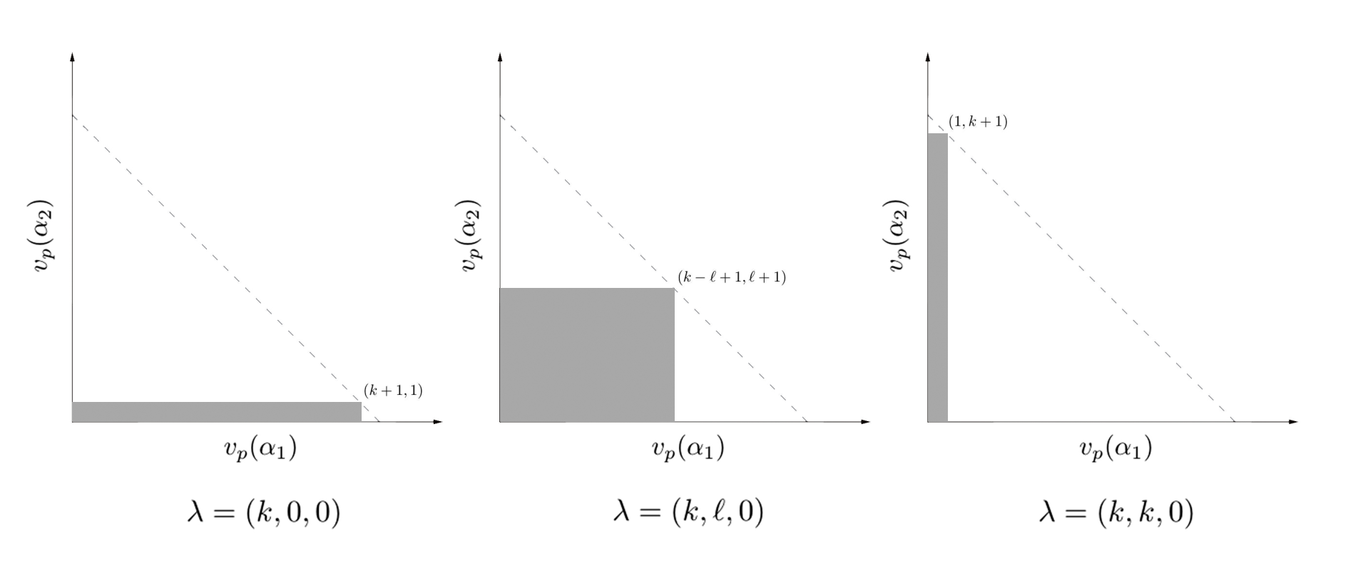
Suppose α1,α2∈𝒪L\alpha_{1},\alpha_{2}\in\mathcal{O}_{L} with vp​(α1)<k1−k2+1v_{p}(\alpha_{1})<k_{1}-k_{2}+1 and vp​(α2)<k2+1.v_{p}(\alpha_{2})<k_{2}+1. Then the restriction

ρλ:Hr​(Γ,𝔻λ​(𝒪L))Up,i=αi→∼Hr​(Γ,Lλ​(𝒪L)Up,i=αiCLOSE\rho_{\lambda}:\mathrm{H}^{r}(\Gamma,\mathbb{D}_{\lambda}(\mathcal{O}_{L}))^{U_{p,i}=\alpha_{i}}\xrightarrow{\,\smash{\raisebox{-1.959pt}{$\scriptstyle\sim$}}\,}\mathrm{H}^{r}(\Gamma,L_{\lambda}(\mathcal{O}_{L})^{U_{p,i}=\alpha_{i}}

of the specialisation map to the simultaneous αi\alpha_{i}-eigenspaces of the Up,iU_{p,i} operators is an isomorphism.

Figure 1: Graphic showing range of lifting for fixed k1=kk_{1}=k and varying k2k_{2} (with dotted line vp​(α1)+vp​(α2)=k+2v_{p}(\alpha_{1})+v_{p}(\alpha_{2})=k+2)

Refer to caption

Summary of argument

We give a brief summary of the argument we use to prove the general lifting theorem. The major component in the proof is showing that the specialisation map is surjective, in the process constructing an explicit lift of any element of the target space. Suppose we start with spaces DD and VV, with actions of a group Γ\Gamma and an operator UU, and suppose that UU also acts naturally on the group cohomology of these spaces. Suppose moreover that we have a surjection pr:D→V\mathrm{pr}:D\rightarrow V that is equivariant with respect to the action of Γ\Gamma and UU, inducing a map ρ\rho on the cohomology. We also assume that we can find a filtration D⊃F0​D⊃F1​D⊃⋯D\supset F^{0}D\supset F^{1}D\supset\cdots such that if we define AN​D   .  .  =D/FN​DA^{N}D\mathrel{\vbox{\hbox{\scriptsize.}\hbox{\scriptsize.}}}=D/F^{N}D, then we have A0​D=VA^{0}D=V. We also suppose that, among other conditions, we have D≅lim←AN​DD\cong\lim_{\leftarrow}A^{N}D. We then start with a UU-eigenclass ϕ0∈H1​(Γ,A0​D)\phi_{0}\in\mathrm{H}^{1}(\Gamma,A^{0}D) with eigenvalue α\alpha. Further assume that α\alpha is an algebraic integer (and hence can be thought of as living in the ring of integers of a finite extension of ℚp\mathbb{Q}_{p}).

  • (i)

    First suppose that ϕ0\phi_{0} is ordinary at pp, that is, suppose α\alpha is a pp-adic unit. Then we take a cocycle φ0\varphi_{0} representing ϕ0\phi_{0}, and lift it to any cochain φ1~:Γ→D\widetilde{\varphi_{1}}:\Gamma\rightarrow D. As α\alpha is a unit, we can apply the operator α−1​U\alpha^{-1}U to this cochain. The magic is that φ1   .  .  =φ1~|α−1​U​(mod​F1​D)\varphi_{1}\mathrel{\vbox{\hbox{\scriptsize.}\hbox{\scriptsize.}}}=\widetilde{\varphi_{1}}|\alpha^{-1}U\hskip 2.0pt(\mathrm{mod}\hskip 2.0ptF^{1}D) is an A1​DA^{1}D-valued cocycle that is independent of choices, and thus defines a canonical lift of ϕ0\phi_{0} to a UU-eigensymbol ϕ1∈H1​(Γ,A1​D)\phi_{1}\in\mathrm{H}^{1}(\Gamma,A^{1}D). Continuing in this vein, we get compatible classes ϕN∈H1​(Γ,AN​D)\phi_{N}\in\mathrm{H}^{1}(\Gamma,A^{N}D) for each NN, and thus an eigenclass in the inverse limit Φ∈H1​(Γ,D)\Phi\in\mathrm{H}^{1}(\Gamma,D) that maps to ϕ0\phi_{0} under ρ\rho.

  • (ii)

    For more general α\alpha, we need a subtler argument. We would like to be able to apply the operator α−1​U\alpha^{-1}U, but since α\alpha need not be a unit, we must strengthen our assumptions. In particular, we need the following:

    • (a)

      A stronger condition on the filtration; namely, if μ∈FN​D,\mu\in F^{N}D, then μ|U∈α​FN+1​D.\mu|U\in\alpha F^{N+1}D.

    • (b)

      An additional piece of data; namely, a Γ\Gamma- and UU-stable submodule DαD^{\alpha} of DD such that if μ∈Dα\mu\in D^{\alpha}, we have μ|U∈α​D\mu|U\in\alpha D.

    The benefit of this is that we can make sense of the operator α−1​U\alpha^{-1}U on cochains that have values in DαD^{\alpha}. We can run morally the same argument as above in this case. Unfortunately, the details of the argument become considerably more technical.

It is natural to ask when such conditions are satisfied. Condition (b) is relatively weak, and it seems reasonable to expect that a submodule DαD^{\alpha} satisfying this condition exists in wider generality; in particular, when DD is a module of pp-adic distributions on a finite number of variables, DαD^{\alpha} can be defined by imposing a simple condition on the low degree moments. Condition (a), however, is stronger, and leads to the notion of small slope. To illustrate this, consider the following examples of cases where such filtrations exist:

  • •

    One can find suitable filtrations in the cases of modular symbols attached to modular forms of weight k+2k+2 over ℚ\mathbb{Q} (see [Gre07]). In this case, condition (a) is satisfied only if vp​(α)<k+1v_{p}(\alpha)<k+1, that is, if the modular form has small slope at pp.

  • •

    A similar result is given for modular forms over an imaginary quadratic field KK in [Wil17]. In the case of weight (k,k)(k,k), and p​𝒪K=𝔭​𝔭¯p\mathcal{O}_{K}=\mathfrak{p}\overline{\mathfrak{p}} split, the natural filtrations for U𝔭U_{\mathfrak{p}} and U𝔭¯U_{\overline{\mathfrak{p}}} satisfy condition (a) (with respect to α𝔭\alpha_{\mathfrak{p}} and α𝔭¯\alpha_{\overline{\mathfrak{p}}}) only if vp​(α𝔭),vp​(α𝔭¯)<k+1.v_{p}(\alpha_{\mathfrak{p}}),v_{p}(\alpha_{\overline{\mathfrak{p}}})<k+1. A more detailed description of these results is given in Section 3.

Structure

In the first section, we describe the set-up of the theorem and the precise properties we require of our filtrations. In the second, we give a proof of our main theorem. In the third, we summarise the case of GL2\mathrm{GL}_{2} over an imaginary quadratic field. In the fourth, we set up the case of SL3\mathrm{SL}_{3} by giving the relevant definitions of the various coefficient spaces and specialisation maps, and finally, in the fifth section, we define the filtrations we require in this case before stating the results for SL3\mathrm{SL}_{3}.

Acknowledgements

I would like to thank Marc Masdeu for encouraging me to publish the lifting theorem contained in this paper. I am also indebted to David Loeffler, as ever, for his very helpful suggestions as I worked on applying this theorem to the case of non-critical slope eigenclasses for SL3\mathrm{SL}_{3}. The author was supported by an EPSRC DTG doctoral grant at the University of Warwick.

1 Setup

Notation 1.1:

Suppose that we have:

  • (i)

    A monoid Σ\Sigma,

  • (ii)

    A group Γ≤Σ\Gamma\leq\Sigma,

  • (iii)

    A ring RR and a right R⁡[Σ]R[\Sigma]-module DD,

  • (iv)

    An R⁡[Σ]R[\Sigma]-stable filtration of DD, given by D⊃ℱ0​D⊃ℱ1​D⊃⋯,D\supset\mathcal{F}^{0}D\supset\mathcal{F}^{1}D\supset\cdots, such that if we define 𝒜N​D   .  .  =D/ℱN​D\mathcal{A}^{N}D\mathrel{\vbox{\hbox{\scriptsize.}\hbox{\scriptsize.}}}=D/\mathcal{F}^{N}D, then we have

    lim⟵𝒜N​D=D,\lim\limits_{\longleftarrow}\mathcal{A}^{N}D=D,

    and where the ℱN​D\mathcal{F}^{N}D have trivial intersection, and

  • (v)

    For some fixed α∈R\alpha\in R, a right Σ\Sigma-stable submodule DαD^{\alpha} of DD, with Vα   .  .  =Im⁡(Dα→𝒜0​D).V^{\alpha}\mathrel{\vbox{\hbox{\scriptsize.}\hbox{\scriptsize.}}}=\mathrm{Im}(D^{\alpha}\rightarrow\mathcal{A}^{0}D).

Note that for each γ∈Σ\gamma\in\Sigma such that Γ\Gamma and γ−1​Γ​γ\gamma^{-1}\Gamma\gamma are commensurable, and any Γ\Gamma-module 𝔻\mathbb{D}, we have an operator UγU_{\gamma} on the cohomology group Hr​(Γ,𝔻)\mathrm{H}^{r}(\Gamma,\mathbb{D}) defined in the usual way, that is, by the composition of the maps

Hr​(Γ,𝔻)→resHr​(Γ∩γ−1​Γ​γ,𝔻)→γHr​(Γ∩γ​Γ​γ−1,𝔻)→coresHr​(Γ,𝔻).\mathrm{H}^{r}(\Gamma,\mathbb{D})\mathrel{\mathop{\xrightarrow{\hskip 28.45274pt}}^{\text{res}}}\mathrm{H}^{r}(\Gamma\cap\gamma^{-1}\Gamma\gamma,\mathbb{D})\mathrel{\mathop{\xrightarrow{\hskip 28.45274pt}}^{\gamma}}\mathrm{H}^{r}(\Gamma\cap\gamma\Gamma\gamma^{-1},\mathbb{D})\mathrel{\mathop{\xrightarrow{\hskip 28.45274pt}}^{\text{cores}}}\mathrm{H}^{r}(\Gamma,\mathbb{D}).
Theorem 1.2.

Suppose that α\alpha is a non-zero element of RR, that DαD^{\alpha} and VαV^{\alpha}and their corresponding cohomology groups have trivial RR-torsion, and that for some π∈Σ\pi\in\Sigma, we have

  • (a)

    If μ∈Dα\mu\in D^{\alpha}, then μ|π∈α​D\mu|\pi\in\alpha D, and

  • (b)

    If μ∈ℱN​D,\mu\in\mathcal{F}^{N}D, then μ|π∈α​ℱN+1​D.\mu|\pi\in\alpha\mathcal{F}^{N+1}D.

Then the restriction of the natural map ρ:Hr​(Γ,Dα)→Hr​(Γ,Vα)\rho:\mathrm{H}^{r}(\Gamma,D^{\alpha})\rightarrow\mathrm{H}^{r}(\Gamma,V^{\alpha}) to the α\alpha-eigenspaces of the UπU_{\pi} operator is an isomorphism.

Remark:

This result is very similar to Theorem 3.1 of [PP09]; their conditions are slightly weaker, but their conclusion requires α\alpha to be a unit. In their case, they do not require the condition on trivial RR-torsion, and then prove that there is a unique eigenlift Φ\Phi of an eigensymbol ϕ\phi that has AnnR​(Φ)=AnnR​(ϕ)\mathrm{Ann}_{R}(\Phi)=\mathrm{Ann}_{R}(\phi). For simplicity, we have imposed this condition to ensure these annihilators are trivial. In the cases we consider, these conditions are satisfied.

We have natural Σ\Sigma-equivariant projection maps

prN:D⟶𝒜N​D\mathrm{pr}^{N}:D\longrightarrow\mathcal{A}^{N}D

that induce Σ\Sigma-equivariant maps

ρN:Hr​(Γ,D)⟶Hr​(Γ,𝒜N​D),\rho^{N}:\mathrm{H}^{r}(\Gamma,D)\longrightarrow\mathrm{H}^{r}(\Gamma,\mathcal{A}^{N}D),

(and hence ρ   .  .  =ρ0:Hr​(Γ,Dα)→Hr​(Γ,Vα)\rho\mathrel{\vbox{\hbox{\scriptsize.}\hbox{\scriptsize.}}}=\rho^{0}:\mathrm{H}^{r}(\Gamma,D^{\alpha})\rightarrow\mathrm{H}^{r}(\Gamma,V^{\alpha}) by restriction) as well as maps prM,N:𝒜M​D→𝒜N​D\mathrm{pr}^{M,N}:\mathcal{A}^{M}D\rightarrow\mathcal{A}^{N}D for M≥NM\geq N that similarly induce maps ρM,N.\rho^{M,N}. Thus we have an inverse system, and we have

lim⟵Hr​(Γ,𝒜N​D)=Hr​(Γ,D).\displaystyle\lim\limits_{\longleftarrow}\mathrm{H}^{r}(\Gamma,\mathcal{A}^{N}D)=\mathrm{H}^{r}(\Gamma,D).

First we pass to a filtration where the Σ\Sigma-action is nicer. Define ℱN​Dα=ℱN​D∩Dα.\mathcal{F}^{N}D^{\alpha}=\mathcal{F}^{N}D\cap D^{\alpha}. This is a Σ\Sigma-stable filtration of DαD^{\alpha}, since DαD^{\alpha} is Σ\Sigma-stable. It’s immediate that if μ∈ℱN​Dα,\mu\in\mathcal{F}^{N}D^{\alpha}, then μ|π∈α​ℱN+1​Dα.\mu|\pi\in\alpha\mathcal{F}^{N+1}D^{\alpha}. Define 𝒜N​Dα=Dα/ℱN​Dα\mathcal{A}^{N}D^{\alpha}=D^{\alpha}/\mathcal{F}^{N}D^{\alpha}, so that we have the following (where the vertical maps are injections): {diagram} Again, we see that

lim⟵Hr​(Γ,𝒜N​Dα)=Hr​(Γ,Dα).\displaystyle\lim\limits_{\longleftarrow}\mathrm{H}^{r}(\Gamma,\mathcal{A}^{N}D^{\alpha})=\mathrm{H}^{r}(\Gamma,D^{\alpha}). (1)
Notation:

(The UU operator at the level of cochains). In [PP09], a description of the U=UπU=U_{\pi} operator at the level of cochains is given. In particular, they take an explicit free resolution

⋯→δ3F2→δ2F1→δ1F0→d0ℤ⟶0\cdots\mathrel{\mathop{\xrightarrow{\hskip 28.45274pt}}^{\delta_{3}}}F_{2}\mathrel{\mathop{\xrightarrow{\hskip 28.45274pt}}^{\delta_{2}}}F_{1}\mathrel{\mathop{\xrightarrow{\hskip 28.45274pt}}^{\delta_{1}}}F_{0}\mathrel{\mathop{\xrightarrow{\hskip 28.45274pt}}^{d_{0}}}\mathbb{Z}\longrightarrow 0

of ℤ\mathbb{Z} by right ℤ⁡[Γ]\mathbb{Z}[\Gamma]-modules; then, for a right ℤ⁡[Γ]\mathbb{Z}[\Gamma]-module 𝔻\mathbb{D}, they use this to explicitly write down the spaces Cr​(Γ,𝔻)   .  .  =HomΓ​(Fr,𝔻)C^{r}(\Gamma,\mathbb{D})\mathrel{\vbox{\hbox{\scriptsize.}\hbox{\scriptsize.}}}=\mathrm{Hom}_{\Gamma}(F_{r},\mathbb{D}) of cochains, Zr(Γ,𝔻)   .  .  =Ker(dr:Cr(Γ,𝔻)→Cr+1(Γ,𝔻)Z^{r}(\Gamma,\mathbb{D})\mathrel{\vbox{\hbox{\scriptsize.}\hbox{\scriptsize.}}}=\mathrm{Ker}(d_{r}:C^{r}(\Gamma,\mathbb{D})\rightarrow C^{r+1}(\Gamma,\mathbb{D}) of cocycles, and Br​(Γ,𝔻)   .  .  =dr−1​(Γ,𝔻)B^{r}(\Gamma,\mathbb{D})\mathrel{\vbox{\hbox{\scriptsize.}\hbox{\scriptsize.}}}=d_{r-1}(\Gamma,\mathbb{D}) of coboundaries, where drd_{r} is the obvious map induced by δr\delta_{r}. Then the group cohomology is defined as Hr​(Γ,𝔻)   .  .  =Zr​(Γ,𝔻)/Br​(Γ,𝔻)\mathrm{H}^{r}(\Gamma,\mathbb{D})\mathrel{\vbox{\hbox{\scriptsize.}\hbox{\scriptsize.}}}=Z^{r}(\Gamma,\mathbb{D})/B^{r}(\Gamma,\mathbb{D}).

Now, F∗π→ℤ→0F_{*}^{\pi}\rightarrow\mathbb{Z}\rightarrow 0 is a free resolution of ℤ⁡[π−1​Γ​π]\mathbb{Z}[\pi^{-1}\Gamma\pi]-modules, and as 𝔽∗→ℤ→0\mathbb{F}_{*}\rightarrow\mathbb{Z}\rightarrow 0 is also a free resolution of ℤ⁡[π−1​Γ​π]\mathbb{Z}[\pi^{-1}\Gamma\pi]-modules, there is a ℤ⁡[π−1​Γ​π]\mathbb{Z}[\pi^{-1}\Gamma\pi]-complex map τ∗\tau_{*} from F∗F_{*} to F∗πF_{*}^{\pi} lifting the identity map on ℤ\mathbb{Z}.

Pick a set {πi}\{\pi_{i}\} of coset representatives for Γ​π\Gamma\pi in Γ​π​Γ\Gamma\pi\Gamma, noting that this is finite by commensurability. Then define U:Hom⁡(Fr,D)→Hom⁡(Fr,D)U:\mathrm{Hom}(F_{r},D)\rightarrow\mathrm{Hom}(F_{r},D) at the level of cochains by

(φ|U)​(fr)   .  .  =∑iφ⁡(τr​(fr⋅πi−1))⋅π​πi,φ∈Hom⁡(Fr,D),fr∈Fr.(\varphi|U)(f_{r})\mathrel{\vbox{\hbox{\scriptsize.}\hbox{\scriptsize.}}}=\sum_{i}\varphi(\tau_{r}(f_{r}\cdot\pi_{i}^{-1}))\cdot\pi\pi_{i},\hskip 12.0pt\varphi\in\mathrm{Hom}(F_{r},D),f_{r}\in F_{r}.

Pollack and Pollack prove (in Lemma 3.2) that this induces a map of chain complexes and hence a map of cohomology groups. In fact, this map is nothing other than UπU_{\pi} as defined above.

Definition.

(UU-eigensymbols of eigenvalue α\alpha). Since 𝒜N​Dα\mathcal{A}^{N}D^{\alpha} may have non-trivial α\alpha-torsion, we should make the statement “UπU_{\pi}-eigensymbol in Hr​(Γ,𝒜N​Dα)\mathrm{H}^{r}(\Gamma,\mathcal{A}^{N}D^{\alpha})” more precise. By condition (a) of 1.2, if μ∈Dα\mu\in D^{\alpha}, then μ|π∈α​D\mu|\pi\in\alpha D. We can thus consider π\pi as a map from DαD^{\alpha} to DD in a natural way, and define another map VπV_{\pi} from DαD^{\alpha} to DD by setting

x|Vπ=y, where x|π=αy.x|V_{\pi}=y,\hskip 12.0pt\text{ where }x|\pi=\alpha y.

We see we have a formal equality of maps α​Vπ=π\alpha V_{\pi}=\pi from DαD^{\alpha} to DD. Thus we get an operator

V   .  .  =Vπ:Hr​(Γ,Dα)⟶Hr​(Γ,D)V\mathrel{\vbox{\hbox{\scriptsize.}\hbox{\scriptsize.}}}=V_{\pi}:\mathrm{H}^{r}(\Gamma,D^{\alpha})\longrightarrow\mathrm{H}^{r}(\Gamma,D)

on the cohomology, so that we have an equality of operators α​V=U\alpha V=U as operators on Hr​(Γ,Dα)\mathrm{H}^{r}(\Gamma,D^{\alpha}). There is also a canonical operator

ε:Hr​(Γ,Dα)⟶Hr​(Γ,D)\varepsilon:\mathrm{H}^{r}(\Gamma,D^{\alpha})\longrightarrow\mathrm{H}^{r}(\Gamma,D)

induced by the inclusion Dα→DD^{\alpha}\rightarrow D. We see that if ϕ∈Hr​(Γ,Dα)\phi\in\mathrm{H}^{r}(\Gamma,D^{\alpha}) satsifies ϕ|U=α​ϕ\phi|U=\alpha\phi, then ε⁡(ϕ)=ϕ|V\varepsilon(\phi)=\phi|V as elements of Hr​(Γ,D)\mathrm{H}^{r}(\Gamma,D).

Remark:

The reason we don’t simply just define V=α−1​UπV=\alpha^{-1}U_{\pi} is that ‘dividing by α\alpha’ is not in general a well-defined notion on DD.

It is easy to see that for each NN, VV gives rise to an operator VN:𝒜N​Dα→𝒜N​DV_{N}:\mathcal{A}^{N}D^{\alpha}\rightarrow\mathcal{A}^{N}D. Denote the canonical map Hr​(Γ,𝒜N​Dα)→Hr​(Γ,𝒜N​D)\mathrm{H}^{r}(\Gamma,\mathcal{A}^{N}D^{\alpha})\rightarrow\mathrm{H}^{r}(\Gamma,\mathcal{A}^{N}D) by εN\varepsilon_{N}. We say an element φN∈Hr​(Γ,𝒜N​Dα)\varphi_{N}\in\mathrm{H}^{r}(\Gamma,\mathcal{A}^{N}D^{\alpha}) is a UU-eigensymbol of eigenvalue α\alpha if εN​(φN)=φN|VN\varepsilon_{N}(\varphi_{N})=\varphi_{N}|V_{N} as elements of Hr​(Γ,𝒜N​D)\mathrm{H}^{r}(\Gamma,\mathcal{A}^{N}D). Henceforth, when we talk about UU-eigensymbols, it shall be assumed that the eigenvalue is α\alpha.

2 Proof of Theorem 1.2

Proof.

(Theorem 1.2). We first prove surjectivity. Take a UU-eigensymbol ϕ0\phi_{0} of eigenvalue α\alpha in Hr​(Γ,Vα)=Hr​(Γ,𝒜0​Dα)\mathrm{H}^{r}(\Gamma,V^{\alpha})=\mathrm{H}^{r}(\Gamma,\mathcal{A}^{0}D^{\alpha}). Suppose there exists a lift ϕN∈Hr​(Γ,𝒜N+1​Dα)\phi_{N}\in\mathrm{H}^{r}(\Gamma,\mathcal{A}^{N+1}D^{\alpha}) of ϕ0\phi_{0} to a UU-eigensymbol for some NN. We prove that we can canonically lift ϕN\phi_{N} to some ϕN+1\phi_{N+1}, and thus we will be done by induction and equation (1), as we have constructed an element in the inverse limit. We prove this in a series of claims.

Take a cocycle φN\varphi_{N} representing ϕN\phi_{N}, and lift it to a cochain φ∈CΓ​(Fr,Dα)\varphi\in C_{\Gamma}(F_{r},D^{\alpha}). We apply VV at the level of cochains, obtaining a cochain φ|V:Fn→D\varphi|V:F_{n}\rightarrow D. Define a cochain

τN+1:Fn⟶𝒜N+1​D\tau_{N+1}:F_{n}\longrightarrow\mathcal{A}^{N+1}D

by composing this with the reduction map. This is in fact a cocycle; as φN\varphi_{N} is a cocycle, d​φd\varphi takes values in ℱN​Dα\mathcal{F}^{N}D^{\alpha}, and thus as we have d⁡(φ|V)=(d​φ)|Vd(\varphi|V)=(d\varphi)|V taking values in ℱN+1​D\mathcal{F}^{N+1}D (by properties of VV), it follows that d​τN+1=0d\tau_{N+1}=0. Thus τN+1\tau_{N+1} represents some cohomology class [τN+1]D∈Hr​(Γ,𝒜N+1​D).[\tau_{N+1}]_{D}\in\mathrm{H}^{r}(\Gamma,\mathcal{A}^{N+1}D).

Claim 2.1.

The cohomology class [τN+1]D[\tau_{N+1}]_{D} is independent of choices.

Proof.

Suppose we take a different cochain φ~\widetilde{\varphi} lifting a different cocycle φN~\widetilde{\varphi_{N}} to a cochain taking values in DαD^{\alpha}. Then [ρN​(φ−φ~)]Dα=0[\rho^{N}(\varphi-\widetilde{\varphi})]_{D^{\alpha}}=0, where ρN\rho^{N} is the natural reduction map, as φN\varphi_{N} and φN~\widetilde{\varphi_{N}} both represent ϕN\phi_{N}. Thus [φ−φ~]Dα∈Hr​(Γ,Dα)[\varphi-\widetilde{\varphi}]_{D^{\alpha}}\in\mathrm{H}^{r}(\Gamma,D^{\alpha}) is represented by a cocycle ψ\psi taking values in ℱN​Dα\mathcal{F}^{N}D^{\alpha}. Therefore [φ−φ~]Dα|V[\varphi-\widetilde{\varphi}]_{D^{\alpha}}|V is represented by ψ|V\psi|V, which by examining the explicit action of UU on cochains we see to take values in ℱN+1​D\mathcal{F}^{N+1}D. After reduction (mod ℱN+1​D\mathcal{F}^{N+1}D), we see that

[τN+1]D−[ρN+1​(φ~|V)]D=[ρN+1​(ψ|V)]D=0,[\tau_{N+1}]_{D}-[\rho^{N+1}(\widetilde{\varphi}|V)]_{D}=[\rho^{N+1}(\psi|V)]_{D}=0,

which is the result. ∎

Claim 2.2.

There exists a cocycle representing [τN+1]D[\tau_{N+1}]_{D} taking values in the smaller space 𝒜N+1​Dα\mathcal{A}^{N+1}D^{\alpha}.

Proof.

As ϕN\phi_{N} is a UU-eigensymbol, we know that as cocycles, φN\varphi_{N} and τN   .  .  =ρN​(φ|V)\tau_{N}\mathrel{\vbox{\hbox{\scriptsize.}\hbox{\scriptsize.}}}=\rho^{N}(\varphi|V) determine the same cohomology class in Hr​(Γ,𝒜N​D)\mathrm{H}^{r}(\Gamma,\mathcal{A}^{N}D). Thus there exists some coboundary bN∈Br​(Γ,𝒜N​D)b_{N}\in B^{r}(\Gamma,\mathcal{A}^{N}D) such that φN=τN+bN\varphi_{N}=\tau_{N}+b_{N}. Then by definition bN=d⁡(cN)b_{N}=d(c_{N}) for some cN∈Cr−1​(Γ,𝒜N​D)c_{N}\in C^{r-1}(\Gamma,\mathcal{A}^{N}D). Lift cNc_{N} arbitrarily to a cochain cN+1∈Cr−1​(Γ,𝒜N+1)c_{N+1}\in C^{r-1}(\Gamma,\mathcal{A}^{N+1}), and define bN+1   .  .  =d⁡(cN+1)∈Br​(Γ,𝒜N+1​D)b_{N+1}\mathrel{\vbox{\hbox{\scriptsize.}\hbox{\scriptsize.}}}=d(c_{N+1})\in B^{r}(\Gamma,\mathcal{A}^{N+1}D). Then

ρN+1,N​(τN+1+bN+1)=τN+bN=φN∈Zr​(Γ,𝒜N​Dα).\rho^{N+1,N}(\tau_{N+1}+b_{N+1})=\tau_{N}+b_{N}=\varphi_{N}\in Z^{r}(\Gamma,\mathcal{A}^{N}D^{\alpha}).

Therefore it follows that φN+1   .  .  =τN+1+bN+1\varphi_{N+1}\mathrel{\vbox{\hbox{\scriptsize.}\hbox{\scriptsize.}}}=\tau_{N+1}+b_{N+1} takes values in the smaller space 𝒜N+1​Dα\mathcal{A}^{N+1}D^{\alpha}. As τN+1+bN+1∈Zr​(Γ,𝒜N+1​D)\tau_{N+1}+b_{N+1}\in Z^{r}(\Gamma,\mathcal{A}^{N+1}D), it follows that φN+1∈Zr​(Γ,Dα)\varphi_{N+1}\in Z^{r}(\Gamma,D^{\alpha}). Thus φN+1\varphi_{N+1} is the required cocycle to prove the claim.

∎

Define ϕN+1   .  .  =[φN+1]Dα∈Hr​(Γ,𝒜N+1​Dα)\phi_{N+1}\mathrel{\vbox{\hbox{\scriptsize.}\hbox{\scriptsize.}}}=[\varphi_{N+1}]_{D^{\alpha}}\in\mathrm{H}^{r}(\Gamma,\mathcal{A}^{N+1}D^{\alpha}) to be the 𝒜N+1​Dα\mathcal{A}^{N+1}D^{\alpha}-valued cohomology class determined by φN+1\varphi_{N+1}.

Claim 2.3.

The cohomology class ϕN+1\phi_{N+1} is independent of all choices.

Proof.

Suppose we choose a different preimage cN~\widetilde{c_{N}} of bNb_{N} under dd, leading to a different cN+1~\widetilde{c_{N+1}} and bN+1~\widetilde{b_{N+1}}, and thus a different φN+1~\widetilde{\varphi_{N+1}}. Then

φN+1−φN+1~=bN+1−bN+1~=d⁡(cN+1−cN+1~).\varphi_{N+1}-\widetilde{\varphi_{N+1}}=b_{N+1}-\widetilde{b_{N+1}}=d(c_{N+1}-\widetilde{c_{N+1}}).

As φN+1−φN+1~\varphi_{N+1}-\widetilde{\varphi_{N+1}} takes values in 𝒜N+1​Dα\mathcal{A}^{N+1}D^{\alpha}, so must cN+1−cN+1~c_{N+1}-\widetilde{c_{N+1}}; hence bN+1−bN+1~∈Br​(Γ,𝒜N+1​Dα)b_{N+1}-\widetilde{b_{N+1}}\in B^{r}(\Gamma,\mathcal{A}^{N+1}D^{\alpha}), so that

[φN+1]Dα=[φN+1~]Dα∈Hr​(Γ,𝒜N+1​Dα).[\varphi_{N+1}]_{D^{\alpha}}=[\widetilde{\varphi_{N+1}}]_{D^{\alpha}}\in\mathrm{H}^{r}(\Gamma,\mathcal{A}^{N+1}D^{\alpha}).

Thus they also determine the same cohomology class, namely [τN+1]D[\tau_{N+1}]_{D}, in Hr​(Γ,𝒜N+1​D).\mathrm{H}^{r}(\Gamma,\mathcal{A}^{N+1}D). As the cohomology class [τN+1]D[\tau_{N+1}]_{D} is also uniquely determined by Claim 2.1, we’re done. ∎

Claim 2.4.

ϕN+1\phi_{N+1} is a UU-eigensymbol with eigenvalue α\alpha.

Proof.

It’s clear that the representative φN+1\varphi_{N+1} of ϕN+1\phi_{N+1} is a lift of φN\varphi_{N}, by definition. Thus any lift φ\varphi of φN+1\varphi_{N+1} to a cochain taking values in DαD^{\alpha} is also a lift of φN\varphi_{N}, and accordingly, it follows that

ϕN+1|VN+1   .  .  =[ρN+1​(φ|V)]D=[τN+1]D.\phi_{N+1}|V_{N+1}\mathrel{\vbox{\hbox{\scriptsize.}\hbox{\scriptsize.}}}=[\rho^{N+1}(\varphi|V)]_{D}=[\tau_{N+1}]_{D}.

Also by definition, φN+1\varphi_{N+1} and τN+1\tau_{N+1} represent the same elements of Hr​(Γ,𝒜N+1​D)\mathrm{H}^{r}(\Gamma,\mathcal{A}^{N+1}D), so that ε⁡(ϕN+1)=[τN+1]D\varepsilon(\phi_{N+1})=[\tau_{N+1}]_{D}. Combining the two equalities gives ε⁡(ϕN+1)=ϕN+1|VN+1\varepsilon(\phi_{N+1})=\phi_{N+1}|V_{N+1}, which is the required result. ∎

Thus we obtain surjectivity. Take some UU-eigensymbol ϕ0∈Hr​(Γ,Vα)=Hr​(Γ,𝒜0​Dα)\phi_{0}\in\mathrm{H}^{r}(\Gamma,V^{\alpha})=\mathrm{H}^{r}(\Gamma,\mathcal{A}^{0}D^{\alpha}), and for each N∈ℕN\in\mathbb{N}, lift it to a UU-eigensymbol ϕN\phi_{N} using the above method. Then we obtain an element of the inverse limit lim←Hr​(Γ,𝒜N​Dα),\lim_{\leftarrow}\mathrm{H}^{r}(\Gamma,\mathcal{A}^{N}D^{\alpha}), which we know is isomorphic in a natural way to Hr​(Γ,Dα)\mathrm{H}^{r}(\Gamma,D^{\alpha}). This element is thus a UU-eigensymbol that maps to ϕ0\phi_{0} under the specialisation map.

It remains to prove injectivity. Suppose ϕ∈ker⁡(ρ)\phi\in\ker(\rho); we aim to show that ϕ=0\phi=0. Consider the exact sequence

0⟶ℱ0​Dα⟶Dα⟶Vα⟶0.0\longrightarrow\mathcal{F}^{0}D^{\alpha}\longrightarrow D^{\alpha}\longrightarrow V^{\alpha}\longrightarrow 0.

This leads to a long exact sequence of cohomology

⋯Hr(Γ,ℱ0Dα)⟶Hr(Γ,Dα)→ρHr(Γ,Vα)⟶⋯,\cdots\mathrm{H}^{r}(\Gamma,\mathcal{F}^{0}D^{\alpha})\longrightarrow\mathrm{H}^{r}(\Gamma,D^{\alpha})\mathrel{\mathop{\xrightarrow{\hskip 28.45274pt}}^{\rho}}\mathrm{H}^{r}(\Gamma,V^{\alpha})\longrightarrow\cdots,

and accordingly any element of ker⁡(ρ)\ker(\rho) must lie in the image of Hr​(Γ,ℱ0​Dα)\mathrm{H}^{r}(\Gamma,\mathcal{F}^{0}D^{\alpha}). This is the same as saying ϕ\phi can be represented by a cocycle φ\varphi taking values in ℱ0​Dα\mathcal{F}^{0}D^{\alpha}. We now conclude using:

Claim 2.5.

Let ϕ∈Hr​(Γ,Dα)\phi\in\mathrm{H}^{r}(\Gamma,D^{\alpha}) be represented by a cocycle φ\varphi taking values in ℱ0​Dα\mathcal{F}^{0}D^{\alpha}. If ϕ\phi is a UU-eigensymbol, then ϕ=0\phi=0.

Proof.

We consider ε⁡(ϕ)=[φ]D\varepsilon(\phi)=[\varphi]_{D}, which is also a UU-eigensymbol. It thus makes sense to apply the operator VV to [φ]D[\varphi]_{D}, for which it is a fixed point. By condition (b) of Theorem 1.2, the VV operator takes ℱN​D\mathcal{F}^{N}D to ℱN+1​D\mathcal{F}^{N+1}D; therefore, as [φ]D[\varphi]_{D} is represented by φ|VN\varphi|V^{N} for any NN (by the eigensymbol property), we see that for each NN, the symbol [φ]D[\varphi]_{D} is represented by a cocycle taking values in ℱN​D\mathcal{F}^{N}D. But the intersection of the ℱN​D\mathcal{F}^{N}D is trivial by assumption. Thus ε⁡(ϕ)=[φ]D\varepsilon(\phi)=[\varphi]_{D} is 0.

It remains to prove that the map ε\varepsilon is injective. We now know that φ\varphi is a coboundary in Cn​(Γ,D)C^{n}(\Gamma,D), so that there exists some c∈Cn−1​(Γ,D)c\in C^{n-1}(\Gamma,D) with φ=d⁡(c)\varphi=d(c). But as φ\varphi takes values in DαD^{\alpha}, it follows that cc must also take values in DαD^{\alpha}. Thus φ\varphi is also a coboundary in Cn​(Γ,Dα)C^{n}(\Gamma,D^{\alpha}), and ϕ=[φ]Dα=0\phi=[\varphi]_{D^{\alpha}}=0, as required. ∎

This completes the proof of Theorem 1.2. ∎

3 Application to GL2×GL2\mathrm{GL}_{2}\times\mathrm{GL}_{2}

As an example of where this theorem applies, we give a brief summary of the case of GL2×GL2\mathrm{GL}_{2}\times\mathrm{GL}_{2}, which is conceptually easier to understand than the case of SL3\mathrm{SL}_{3}. In particular, we present the results in a concrete setting in the style of [Wil17], where these results were first proved. Recall the set-up:

Notation:

Let KK be an imaginary quadratic field with ring of integers 𝒪K\mathcal{O}_{K}, and let pp be a rational prime that splits as 𝔭​𝔭¯\mathfrak{p}\overline{\mathfrak{p}} in KK. Let Γ⊂Γ0​(p)⊂SL2​(𝒪K)\Gamma\subset\Gamma_{0}(p)\subset\mathrm{SL}_{2}(\mathcal{O}_{K}) be a congruence subgroup. Let Σ\Sigma denote the set of complex embeddings of KK, and let λ=(k,k)∈Z⁡[Σ]\lambda=(k,k)\in Z[\Sigma] be a weight, where kk is non-negative. Let L/ℚpL/\mathbb{Q}_{p} be a finite extension with ring of integers 𝒪L\mathcal{O}_{L}.

3.1 Coefficient Modules

Definition 3.1.

Let Vk​(𝒪L)   .  .  =Symk​(𝒪L2)V_{k}(\mathcal{O}_{L})\mathrel{\vbox{\hbox{\scriptsize.}\hbox{\scriptsize.}}}=\mathrm{Sym}^{k}(\mathcal{O}_{L}^{2}) be the space of homogeneous polynomials in two variables of degree kk over 𝒪L\mathcal{O}_{L}.

We can identify Vk​(𝒪L)⊗Vk​(𝒪L)V_{k}(\mathcal{O}_{L})\otimes V_{k}(\mathcal{O}_{L}) with a space of polynomial functions on 𝒪K⊗ℤℤp\mathcal{O}_{K}\otimes_{\mathbb{Z}}\mathbb{Z}_{p} in a natural way.

Definition 3.2.

Let 𝔸k​(𝒪L)   .  .  =𝒪L​⟨z⟩\mathbb{A}_{k}(\mathcal{O}_{L})\mathrel{\vbox{\hbox{\scriptsize.}\hbox{\scriptsize.}}}=\mathcal{O}_{L}\langle z\rangle be the Tate algebra over 𝒪L\mathcal{O}_{L}, that is, the space of power series in one variable whose coefficients tend to zero as the degree tends to infinity.

Remark:

For ease of notation, we will henceforth drop 𝒪L\mathcal{O}_{L} from the notation. All tensor products are over 𝒪L\mathcal{O}_{L}.

Let Σ0​(p)⊂M2​(𝒪L)∩GL2​(L)\Sigma_{0}(p)\subset M_{2}(\mathcal{O}_{L})\cap\mathrm{GL}_{2}(L) be the set of matrices that are upper-triangular modulo pp. In particular, we have Γ⊂Σ0​(p)\Gamma\subset\Sigma_{0}(p). Then 𝔸k\mathbb{A}_{k} has a natural left action of Σ0​(p)\Sigma_{0}(p), depending on kk (justifying the notation), given by

(abcd)⋅f⁡(z)=(a+c​z)k​f​(b+d​za+c​z).\begin{pmatrix}a&b\\ c&d\end{pmatrix}\cdot f(z)=(a+cz)^{k}f\left(\frac{b+dz}{a+cz}\right).

This action preserves the subspace VkV_{k} and hence gives rise to component-wise actions of Σ0​(p)2\Sigma_{0}(p)^{2} on Vk⊗VkV_{k}\otimes V_{k}, Vk⊗𝔸kV_{k}\otimes\mathbb{A}_{k} and 𝔸k⊗𝔸k\mathbb{A}_{k}\otimes\mathbb{A}_{k}. Accordingly, we get right actions of Σ0​(p)2\Sigma_{0}(p)^{2} on their corresponding topological duals Vk∗⊗Vk∗V_{k}^{*}\otimes V_{k}^{*}, Vk∗⊗𝔻kV_{k}^{*}\otimes\mathbb{D}_{k} and 𝔻k​⊗^​𝔻k\mathbb{D}_{k}\widehat{\otimes}\mathbb{D}_{k} respectively. By dualising the inclusions, we get Σ0​(p)2\Sigma_{0}(p)^{2}-equivariant surjections

𝔻k​⊗^​𝔻k→pr2Vk∗⊗𝔻k→pr1Vk∗⊗Vk∗,\mathbb{D}_{k}\widehat{\otimes}\mathbb{D}_{k}\mathrel{\mathop{\xrightarrow{\hskip 28.45274pt}}^{\mathrm{pr}_{2}}}V_{k}^{*}\otimes\mathbb{D}_{k}\mathrel{\mathop{\xrightarrow{\hskip 28.45274pt}}^{\mathrm{pr}_{1}}}V_{k}^{*}\otimes V_{k}^{*},

that induce maps

H1​(Γ,𝔻k​⊗^​𝔻k)→ρ2H1​(Γ,Vk∗⊗𝔻k)→ρ1H1​(Γ,Vk∗⊗Vk∗)\mathrm{H}^{1}(\Gamma,\mathbb{D}_{k}\widehat{\otimes}\mathbb{D}_{k})\mathrel{\mathop{\xrightarrow{\hskip 28.45274pt}}^{\rho_{2}}}\mathrm{H}^{1}(\Gamma,V_{k}^{*}\otimes\mathbb{D}_{k})\mathrel{\mathop{\xrightarrow{\hskip 28.45274pt}}^{\rho_{1}}}\mathrm{H}^{1}(\Gamma,V_{k}^{*}\otimes V_{k}^{*})

on the cohomology. We define filtrations as follows:

Definition 3.3.
  • (i)

    Let NN be an integer and define ℱN​𝔻k   .  .  ={μ∈𝔻k:μ⁡(zr)∈πLN−r​𝒪L}\mathcal{F}^{N}\mathbb{D}_{k}\mathrel{\vbox{\hbox{\scriptsize.}\hbox{\scriptsize.}}}=\{\mu\in\mathbb{D}_{k}:\mu(z^{r})\in\pi_{L}^{N-r}\mathcal{O}_{L}\}, where πL\pi_{L} is a uniformiser in 𝒪L\mathcal{O}_{L}. Then define

    ℱN​[Vk∗⊗𝔻k]   .  .  =Vk∗⊗ℱN​𝔻k.\mathcal{F}^{N}[V_{k}^{*}\otimes\mathbb{D}_{k}]\mathrel{\vbox{\hbox{\scriptsize.}\hbox{\scriptsize.}}}=V_{k}^{*}\otimes\mathcal{F}^{N}\mathbb{D}_{k}.

    This is Σ0​(p)\Sigma_{0}(p)-stable by arguments in [Gre07] and [Wil17]. Now define

    FN​[Vk∗⊗𝔻k]   .  .  =ℱN​[Vk∗⊗𝔻k]∩ker⁡(pr1),F^{N}[V_{k}^{*}\otimes\mathbb{D}_{k}]\mathrel{\vbox{\hbox{\scriptsize.}\hbox{\scriptsize.}}}=\mathcal{F}^{N}[V_{k}^{*}\otimes\mathbb{D}_{k}]\cap\ker(\mathrm{pr}_{1}),

    which is also Σ0​(p)\Sigma_{0}(p)-stable as pr1\mathrm{pr}_{1} is Σ0​(p)\Sigma_{0}(p)-equivariant.

  • (ii)

    Similarly, define FN​[𝔻k​⊗^​𝔻k]   .  .  =(ℱN​𝔻k​⊗^​𝔻k)∩ker⁡(pr2),F^{N}[\mathbb{D}_{k}\widehat{\otimes}\mathbb{D}_{k}]\mathrel{\vbox{\hbox{\scriptsize.}\hbox{\scriptsize.}}}=(\mathcal{F}^{N}\mathbb{D}_{k}\widehat{\otimes}\mathbb{D}_{k})\cap\ker(\mathrm{pr}_{2}), which again is Σ0​(p)\Sigma_{0}(p)-stable.

Let α∈𝒪L\alpha\in\mathcal{O}_{L} and let π𝔭   .  .  =[(1001),(100p)]\pi_{\mathfrak{p}}\mathrel{\vbox{\hbox{\scriptsize.}\hbox{\scriptsize.}}}=[\left(\begin{smallmatrix}1&0\\ 0&1\end{smallmatrix}\right),\left(\begin{smallmatrix}1&0\\ 0&p\end{smallmatrix}\right)] and π𝔭¯   .  .  =[(100p),(1001)]∈Σ0​(p)2.\pi_{\overline{\mathfrak{p}}}\mathrel{\vbox{\hbox{\scriptsize.}\hbox{\scriptsize.}}}=[\left(\begin{smallmatrix}1&0\\ 0&p\end{smallmatrix}\right),\left(\begin{smallmatrix}1&0\\ 0&1\end{smallmatrix}\right)]\in\Sigma_{0}(p)^{2}. First, we have:

Lemma 3.4.

Suppose vp​(α)<k+1v_{p}(\alpha)<k+1. Then we have

  • (i)

    If μ∈FN​[Vk∗⊗𝔻k]\mu\in F^{N}[V_{k}^{*}\otimes\mathbb{D}_{k}], then μ|π𝔭∈α​FN+1​[Vk∗⊗𝔻k].\mu|\pi_{\mathfrak{p}}\in\alpha F^{N+1}[V_{k}^{*}\otimes\mathbb{D}_{k}].

  • (ii)

    If μ∈FN​[𝔻k​⊗^​𝔻k]\mu\in F^{N}[\mathbb{D}_{k}\widehat{\otimes}\mathbb{D}_{k}], then μ|π𝔭¯∈α​FN+1​[𝔻k​⊗^​𝔻k].\mu|\pi_{\overline{\mathfrak{p}}}\in\alpha F^{N+1}[\mathbb{D}_{k}\widehat{\otimes}\mathbb{D}_{k}].

We then define the analogue of the module DαD^{\alpha} as follows:

Definition 3.5.
  • (i)

    Define 𝔻kα   .  .  ={μ∈𝔻k:μ⁡(zr)∈α​p−r​𝒪L}\mathbb{D}_{k}^{\alpha}\mathrel{\vbox{\hbox{\scriptsize.}\hbox{\scriptsize.}}}=\{\mu\in\mathbb{D}_{k}:\mu(z^{r})\in\alpha p^{-r}\mathcal{O}_{L}\}, and then define

    [Vk∗⊗𝔻k]α   .  .  =Vk∗⊗𝔻kα.[V_{k}^{*}\otimes\mathbb{D}_{k}]^{\alpha}\mathrel{\vbox{\hbox{\scriptsize.}\hbox{\scriptsize.}}}=V_{k}^{*}\otimes\mathbb{D}_{k}^{\alpha}.
  • (ii)

    Similarly, define [𝔻k​⊗^​𝔻k]α   .  .  =𝔻kα​⊗^​𝔻k[\mathbb{D}_{k}\widehat{\otimes}\mathbb{D}_{k}]^{\alpha}\mathrel{\vbox{\hbox{\scriptsize.}\hbox{\scriptsize.}}}=\mathbb{D}_{k}^{\alpha}\widehat{\otimes}\mathbb{D}_{k}.

Lemma 3.6.
  • (i)

    If μ∈[Vk∗⊗𝔻k]α\mu\in[V_{k}^{*}\otimes\mathbb{D}_{k}]^{\alpha}, then μ|π𝔭∈α​Vk∗⊗𝔻k.\mu|\pi_{\mathfrak{p}}\in\alpha V_{k}^{*}\otimes\mathbb{D}_{k}.

  • (ii)

    If μ∈[𝔻k​⊗^​𝔻k]α\mu\in[\mathbb{D}_{k}\widehat{\otimes}\mathbb{D}_{k}]^{\alpha}, then μ|π𝔭¯∈α​𝔻k​⊗^​𝔻k.\mu|\pi_{\overline{\mathfrak{p}}}\in\alpha\mathbb{D}_{k}\widehat{\otimes}\mathbb{D}_{k}.

Accordingly, we can lift using Theorem 1.2, first along ρ1\rho_{1} using the operator U𝔭U_{\mathfrak{p}} induced by π𝔭\pi_{\mathfrak{p}}, and secondly along ρ2\rho_{2} using the operator U𝔭¯U_{\overline{\mathfrak{p}}} induced by π𝔭¯\pi_{\overline{\mathfrak{p}}}. In particular, we have:

Theorem 3.7.

Let α𝔭,α𝔭¯∈𝒪L\alpha_{\mathfrak{p}},\alpha_{\overline{\mathfrak{p}}}\in\mathcal{O}_{L} with vp​(α1),vp​(α2)<k+1.v_{p}(\alpha_{1}),v_{p}(\alpha_{2})<k+1. Then the restriction of the map ρ   .  .  =ρ2​ρ1\rho\mathrel{\vbox{\hbox{\scriptsize.}\hbox{\scriptsize.}}}=\rho_{2}\rho_{1} to the simultaneous α𝔭\alpha_{\mathfrak{p}} and α𝔭¯\alpha_{\overline{\mathfrak{p}}} eigenspaces of the U𝔭U_{\mathfrak{p}} and U𝔭¯U_{\overline{\mathfrak{p}}} operators respectively is an isomorphism.

Remarks:
  • (i)

    In [Wil17], these results are used to construct pp-adic LL-functions for automorphic forms for GL2\mathrm{GL}_{2} over an imaginary quadratic field, in the spirit of [PS11]. In particular, we associate to such an automorphic form a canonical element in the overconvergent cohomology, from which we can very naturally build a ray class distribution that interpolates LL-values of the automorphic form. It would be interesting to know if similar results existed in the case of SL3\mathrm{SL}_{3}.

  • (ii)

    In the interests of transition to the case of SL3\mathrm{SL}_{3}, we can rephrase the above definitions in a more abstract way. In particular, let G   .  .  =ResK/ℚ​GL2G\mathrel{\vbox{\hbox{\scriptsize.}\hbox{\scriptsize.}}}=\mathrm{Res}_{K/\mathbb{Q}}\mathrm{GL}_{2}, with Borel subgroup BB and opposite Borel BoppB^{\mathrm{opp}}. Define TT to be the torus, and note we can view λ\lambda as a dominant weight for TT, and that Vk⊗VkV_{k}\otimes V_{k} is the representation of GL2\mathrm{GL}_{2} of highest weight λ\lambda with respect to BoppB^{\mathrm{opp}}. Note that for an extension L/ℚpL/\mathbb{Q}_{p}, we have G⁡(L)≅GL2​(L)×GL2​(L)G(L)\cong\mathrm{GL}_{2}(L)\times\mathrm{GL}_{2}(L). Then 𝔸k​⊗^​𝔸k\mathbb{A}_{k}\widehat{\otimes}\mathbb{A}_{k} is the ring of analytic functions on B⁡(L)B(L) that transform like λ\lambda under multiplication by elements of T⁡(L)T(L), whilst Vk⊗𝔸kV_{k}\otimes\mathbb{A}_{k} is the ring of analytic functions on B⁡(L)B(L) that transform like λ\lambda under multiplication by elements of GL2​(L)×Tℚ​(L)\mathrm{GL}_{2}(L)\times T_{\mathbb{Q}}(L), where Tℚ​(L)T_{\mathbb{Q}}(L) is the torus of diagonal matrices in the algebraic group GL2/ℚ\mathrm{GL}_{2}/\mathbb{Q}. In particular, the definitions in the following section are a natural analogue of the theory described concretely above.

4 Overconvergent modular symbols for SL3\mathrm{SL}_{3}

We now apply the results above to give a generalisation of the lifting theorem for SL3\mathrm{SL}_{3} of Pollack and Pollack in [PP09]. We first recall the setting, and also develop the notion of ‘partially overconvergent’ modular symbols for SL3\mathrm{SL}_{3}.

4.1 Notation

We recall the setting; where possible, we keep to the notation used by Pollack and Pollack in [PP09] for clarity. For further details, the reader is directed to their paper. Let GG be the algebraic group GL3/ℚ\mathrm{GL}_{3}/\mathbb{Q}, and denote by BB (resp. BoppB^{\mathrm{opp}}) its Borel subgroup of upper-triangular (resp. lower-triangular) matrices, with TT and NN (resp. NoppN^{\mathrm{opp}}) the subgroups of BB (resp. BoppB^{\mathrm{opp}}) consisting of the diagonal and unipotent matrices respectively. Note that B=T​NB=TN. Let pp be a prime, let Γ0​(p)\Gamma_{0}(p) be the subgroup of SL3​(ℤ)\mathrm{SL}_{3}(\mathbb{Z}) of matrices that are upper-triangular modulo pp, and let Γ\Gamma be a congruence subgroup of SL3​(ℤ)\mathrm{SL}_{3}(\mathbb{Z}) contained in Γ0​(p)\Gamma_{0}(p).

4.2 Classical coefficient modules

Let λ\lambda be a dominant algebraic character of the torus TT, which can be seen as an element λ=(k1,k2,k3)∈ℤ3.\lambda=(k_{1},k_{2},k_{3})\in\mathbb{Z}^{3}. Let VλV_{\lambda} be the (unique) representation of GG with highest weight λ\lambda with respect to BoppB^{\mathrm{opp}}; for example, when λ=(k,0,0)\lambda=(k,0,0), we see that Vλ​(A)V_{\lambda}(A) is nothing but Symk​(A3)\mathrm{Sym}^{k}(A^{3}), for a suitable coefficient module AA.

Remark:

We will restrict to the case where λ=(k1,k2,0)\lambda=(k_{1},k_{2},0), rescaling by the determinant, since this slightly simplifies the calculations. Indeed, any such weight can be written in the form λ=(k1+v,k2+v,v)\lambda=(k_{1}+v,k_{2}+v,v), and then Vλ≅Vλ′⊗detvV_{\lambda}\cong V_{\lambda^{\prime}}\otimes\det^{v}, where λ′=(k1,k2,0)\lambda^{\prime}=(k_{1},k_{2},0). All of our main results then go through in the general case with only slight modification, and indeed, the range of ‘non-criticality’ for the slope for λ′\lambda^{\prime} is the same as that for λ\lambda scaled by vv in each component.

4.3 Overconvergent coefficient modules

We denote by ℂp\mathbb{C}_{p} the completion of fixed algebraic closure of ℚp\mathbb{Q}_{p}, and write 𝒪ℂp\mathcal{O}_{\mathbb{C}_{p}} for its ring of integers. We now define two different overconvergent coefficient modules corresponding to two different parabolic subgroups of SL3\mathrm{SL}_{3}.

4.3.1 Overconvergent with respect to T=SL13T=\mathrm{SL}_{1}^{3}

We first look at the case where we consider the parabolic subgroup T=SL1×SL1×SL1.T=\mathrm{SL}_{1}\times\mathrm{SL}_{1}\times\mathrm{SL}_{1}. This identically mirrors the work of Pollack and Pollack in [PP09]. In particular, let ℐ\mathcal{I} denote the subgroup of G⁡(𝒪ℂp)G(\mathcal{O}_{\mathbb{C}_{p}}) of matrices that are upper-triangular modulo the maximal ideal of 𝒪ℂp\mathcal{O}_{\mathbb{C}_{p}}. We consider continuous function f:B⁡(𝒪ℂp)→𝒪ℂpf:B(\mathcal{O}_{\mathbb{C}_{p}})\rightarrow\mathcal{O}_{\mathbb{C}_{p}} satisfying the condition

f⁡(t​b)=λ⁡(t)​f​(b),t∈T⁡(𝒪ℂp),b∈B⁡(𝒪ℂp)f(tb)=\lambda(t)f(b),\hskip 12.0ptt\in T(\mathcal{O}_{\mathbb{C}_{p}}),b\in B(\mathcal{O}_{\mathbb{C}_{p}}) (2)

We note that any such function is determined by its restriction to N⁡(𝒪ℂp)N(\mathcal{O}_{\mathbb{C}_{p}}), and that we can identify N⁡(𝒪ℂp)N(\mathcal{O}_{\mathbb{C}_{p}}) with 𝒪ℂp3\mathcal{O}_{\mathbb{C}_{p}}^{3} by identifying

(1xy01z001)⟷(x,y,z)∈𝒪ℂp3.\begin{pmatrix}1&x&y\\ 0&1&z\\ 0&0&1\end{pmatrix}\longleftrightarrow(x,y,z)\in\mathcal{O}_{\mathbb{C}_{p}}^{3}.

We write f⁡(x,y,z)f(x,y,z) for the image of this matrix under ff. Let L/ℚpL/\mathbb{Q}_{p} be a finite extension with ring of integers 𝒪L\mathcal{O}_{L}. We say that such a function ff is LL-rigid analytic if, for (x,y,z)∈N⁡(𝒪ℂp)(x,y,z)\in N(\mathcal{O}_{\mathbb{C}_{p}}), we can write ff in the form

f⁡(x,y,z)=∑r,s,t≥0cr​s​t​xr​ys​zt,f(x,y,z)=\sum_{r,s,t\geq 0}c_{rst}x^{r}y^{s}z^{t},

where cr​s​t∈Lc_{rst}\in L tends to 00 as r+s+t→∞r+s+t\rightarrow\infty. Alternatively, this occurs if and only if f⁡(x,y,z)∈L⁡⟨x,y,z⟩f(x,y,z)\in L\langle x,y,z\rangle, the Tate algebra in three variables over LL. Writing 𝒪L\mathcal{O}_{L} for the ring of integers of LL, there is likewise an integral version with cr​s​t∈𝒪L.c_{rst}\in\mathcal{O}_{L}.

Remark:

Henceforth, we will state all definitions and results in terms of coefficients in 𝒪L\mathcal{O}_{L}, since in the sequel we use this integrality in an essential way to define filtrations. We could easily instead state the definitions using LL in place of 𝒪L\mathcal{O}_{L}.

Definition 4.1.
  • (i)

    Write 𝔸λ​(𝒪L)\mathbb{A}_{\lambda}(\mathcal{O}_{L}) for the space of 𝒪L\mathcal{O}_{L}-rigid analytic functions on B⁡(𝒪ℂp)B(\mathcal{O}_{\mathbb{C}_{p}}) that satisfy equation (2).

  • (ii)

    Let 𝔻λ​(𝒪L)\mathbb{D}_{\lambda}(\mathcal{O}_{L}) denote the topological dual

    𝔻λ​(𝒪L)   .  .  =Homcts​(𝔸λ​(𝒪L),𝒪L)\mathbb{D}_{\lambda}(\mathcal{O}_{L})\mathrel{\vbox{\hbox{\scriptsize.}\hbox{\scriptsize.}}}=\mathrm{Hom}_{\mathrm{cts}}(\mathbb{A}_{\lambda}(\mathcal{O}_{L}),\mathcal{O}_{L})

    (resp. Homcts​(𝔸λ​(𝒪L),𝒪L)\mathrm{Hom}_{\mathrm{cts}}(\mathbb{A}_{\lambda}(\mathcal{O}_{L}),\mathcal{O}_{L})), the space of rigid analytic distributions on B⁡(𝒪ℂp)B(\mathcal{O}_{\mathbb{C}_{p}}) of weight λ\lambda.

In an abuse of notation, we write xr​ys​ztx^{r}y^{s}z^{t} for the unique extension to B⁡(𝒪ℂp)B(\mathcal{O}_{\mathbb{C}_{p}}) of the function on N⁡(𝒪ℂp)N(\mathcal{O}_{\mathbb{C}_{p}}) that sends

(1xy01z001)⟼xr​ys​zt,\begin{pmatrix}1&x&y\\ 0&1&z\\ 0&0&1\end{pmatrix}\longmapsto x^{r}y^{s}z^{t},

and note that any μ∈𝔻λ​(𝒪L)\mu\in\mathbb{D}_{\lambda}(\mathcal{O}_{L}) is uniquely determined by its values at xr​ys​ztx^{r}y^{s}z^{t} for r,s,t≥0r,s,t\geq 0. Pollack and Pollack call this function fr​s​tf_{rst}.

4.3.2 Overconvergent with respect to P   .  .  =SL1×SL2P\mathrel{\vbox{\hbox{\scriptsize.}\hbox{\scriptsize.}}}=\mathrm{SL}_{1}\times\mathrm{SL}_{2}

We now define a different module of overconvergent coefficients. This is, in a sense, a smaller module of coefficients, and will play the role of ‘half-overconvergent’ coefficients in the following. Let P=SL1×SL2⊂SL3P=\mathrm{SL}_{1}\times\mathrm{SL}_{2}\subset\mathrm{SL}_{3}. If λ=(k1,k2,0)\lambda=(k_{1},k_{2},0) with k1≥k2k_{1}\geq k_{2}, we get an associated representation

Wλ​(A)   .  .  =detk1⊗Symk2​(A2)W_{\lambda}(A)\mathrel{\vbox{\hbox{\scriptsize.}\hbox{\scriptsize.}}}=\mathrm{det}^{k_{1}}\otimes\hskip 1.0pt\mathrm{Sym}^{k_{2}}(A^{2})

of P⁡(A)=SL1​(A)×SL2​(A)P(A)=\mathrm{SL}_{1}(A)\times\mathrm{SL}_{2}(A), for suitable AA. We can replace BB with the larger subgroup B1B_{1} of matrices that are block lower-triangular with respect to this parabolic subgroup – that is, matrices that are zero in the (2,1)(2,1) and (3,1)(3,1) entries – and consider the space of functions f:B1​(𝒪ℂp)⟶Wλ​(𝒪ℂp)f:B_{1}(\mathcal{O}_{\mathbb{C}_{p}})\longrightarrow W_{\lambda}(\mathcal{O}_{\mathbb{C}_{p}}) satisfying the condition

f⁡(t​g)=λ⁡(t)​f​(g)∀t∈P⁡(𝒪ℂp),g∈B1​(𝒪ℂp),where ​λ​(t)∈GL⁡(Wλ).f(tg)=\lambda(t)f(g)\hskip 12.0pt\forall t\in P(\mathcal{O}_{\mathbb{C}_{p}}),g\in B_{1}(\mathcal{O}_{\mathbb{C}_{p}}),\hskip 20.0pt\text{where }\lambda(t)\in\mathrm{GL}(W_{\lambda}).

Note that any such function is entirely determined by its restriction to B⁡(𝒪ℂp)B(\mathcal{O}_{\mathbb{C}_{p}}), and indeed by its values on the subgroup

{(1xy010001)∈B1(𝒪ℂp)},\left\{\begin{pmatrix}1&x&y\\ 0&1&0\\ 0&0&1\end{pmatrix}\in B_{1}(\mathcal{O}_{\mathbb{C}_{p}})\right\},

by a similar argument to before. We say such a function is 𝒪L\mathcal{O}_{L}-rigid analytic if it is an element of 𝒪L​⟨x,y⟩⊗LWλ​(L)\mathcal{O}_{L}\langle x,y\rangle\otimes_{L}W_{\lambda}(L).

Definition 4.2.

Write 𝔸λP​(𝒪L)\mathbb{A}_{\lambda}^{P}(\mathcal{O}_{L}) for the space of 𝒪L\mathcal{O}_{L}-rigid analytic functions on B1​(𝒪ℂp)B_{1}(\mathcal{O}_{\mathbb{C}_{p}}) that transform like λ\lambda under elements of PP.

Proposition 4.3.

Let f∈𝔸λP​(𝒪L)f\in\mathbb{A}_{\lambda}^{P}(\mathcal{O}_{L}). For g∈Bg\in B, let Pg​(X,Y)   .  .  =f⁡(g)∈Wλ​(𝒪L),P_{g}(X,Y)\mathrel{\vbox{\hbox{\scriptsize.}\hbox{\scriptsize.}}}=f(g)\in W_{\lambda}(\mathcal{O}_{L}), where we consider elements of WλW_{\lambda} as homogeneous polynomials of degree k2k_{2} in two variables over 𝒪L\mathcal{O}_{L}. Define a function

f′:B⁡(𝒪ℂp)⟶𝒪ℂpf^{\prime}:B(\mathcal{O}_{\mathbb{C}_{p}})\longrightarrow\mathcal{O}_{\mathbb{C}_{p}}

by f′​(g)=Pg​(0,1)f^{\prime}(g)=P_{g}(0,1). Then f′∈𝔸λ​(𝒪L)f^{\prime}\in\mathbb{A}_{\lambda}(\mathcal{O}_{L}). Moreover, the association f↦f′f\mapsto f^{\prime} gives an isomorphism

𝔸λP​(𝒪L)→∼{f⁡(x,y,z)=∑r,s,t≥0αr,s,t​xr​ys​zt∈𝔸λ​(𝒪L):αr,s,t=0​ for ​t>k2}.\mathbb{A}_{\lambda}^{P}(\mathcal{O}_{L})\xrightarrow{\,\smash{\raisebox{-1.959pt}{$\scriptstyle\sim$}}\,}\bigg\{f(x,y,z)=\sum_{r,s,t\geq 0}\alpha_{r,s,t}x^{r}y^{s}z^{t}\in\mathbb{A}_{\lambda}(\mathcal{O}_{L}):\alpha_{r,s,t}=0\text{ for }t>k_{2}\bigg\}.
Proof.

Firstly, note that f′f^{\prime} is rigid analytic in three variables. In particular, let

g   .  .  =(1xy010001)andPg(X,Y)=∑t=1k2∑r,s≥0αr,s,txrysXtYk2−t,g\mathrel{\vbox{\hbox{\scriptsize.}\hbox{\scriptsize.}}}=\begin{pmatrix}1&x&y\\ 0&1&0\\ 0&0&1\end{pmatrix}\hskip 12.0pt\text{and}\hskip 12.0ptP_{g}(X,Y)=\sum_{t=1}^{k_{2}}\sum_{r,s\geq 0}\alpha_{r,s,t}x^{r}y^{s}X^{t}Y^{k_{2}-t},

using rigidity of ff. Then consider

g′   .  .  =(1xy01z001)=(10001z001)​(1xy010001).g^{\prime}\mathrel{\vbox{\hbox{\scriptsize.}\hbox{\scriptsize.}}}=\begin{pmatrix}1&x&y\\ 0&1&z\\ 0&0&1\end{pmatrix}=\begin{pmatrix}1&0&0\\ 0&1&z\\ 0&0&1\end{pmatrix}\begin{pmatrix}1&x&y\\ 0&1&0\\ 0&0&1\end{pmatrix}.

Recall that GL2​(L)\mathrm{GL}_{2}(L) acts on Wλ​(L)W_{\lambda}(L) by w|(abcd)​(X,Y)=w⁡(b​Y+d​X,a​Y+c​X),w|\left(\begin{smallmatrix}a&b\\ c&d\end{smallmatrix}\right)(X,Y)=w(bY+dX,aY+cX), so that

f′​(x,y,z)=Pg′​(0,1)=Pg​(X+z,Y)|X=0,Y=1=Pg​(z,1)=∑t=1k2∑r,s≥0αr,s,t​xr​ys​zt.f^{\prime}(x,y,z)=P_{g^{\prime}}(0,1)=P_{g}(X+z,Y)\bigg|_{X=0,Y=1}=P_{g}(z,1)=\sum_{t=1}^{k_{2}}\sum_{r,s\geq 0}\alpha_{r,s,t}x^{r}y^{s}z^{t}. (3)

The rigidity follows. Now we show that f′f^{\prime} transforms under TT as λ\lambda. Let g∈B⁡(𝒪ℂp)g\in B(\mathcal{O}_{\mathbb{C}_{p}}) and t=(t1,t2,t3)∈T⁡(𝒪ℂp)t=(t_{1},t_{2},t_{3})\in T(\mathcal{O}_{\mathbb{C}_{p}}). Then compute

Pt​g​(X,Y)=f⁡(t​g)​(X,Y)=t1k1​f​(g)​(t3​X,t2​Y)=t1k1​Pg​(t3​X,t2​Y).P_{tg}(X,Y)=f(tg)(X,Y)=t_{1}^{k_{1}}f(g)(t_{3}X,t_{2}Y)=t_{1}^{k_{1}}P_{g}(t_{3}X,t_{2}Y).

Accordingly, we have

f′​(t​g)=Pt​g​(0,1)=t1k1​Pg​(0,t2)=t1k1​t2k2​Pg​(0,1)=λ⁡(t)​f′​(g),\displaystyle f^{\prime}(tg)=P_{tg}(0,1)=t_{1}^{k_{1}}P_{g}(0,t_{2})=t_{1}^{k_{1}}t_{2}^{k_{2}}P_{g}(0,1)=\lambda(t)f^{\prime}(g),

as required. Finally, it remains to show that the map induces the stated isomorphism. From equation (3), it is clear that f′=0f^{\prime}=0 if and only if f=0f=0, so that the association f↦f′f\mapsto f^{\prime} is injective. It is also clear that the image is the right-hand side of the isomorphism. This completes the proof. ∎

Definition 4.4.
  • (i)

    From now on, in an abuse of notation using this isomorphism, we write 𝔸λP​(𝒪L)\mathbb{A}_{\lambda}^{P}(\mathcal{O}_{L}) for this subspace of 𝔸λ​(𝒪L)\mathbb{A}_{\lambda}(\mathcal{O}_{L}).

  • (ii)

    Let 𝔻λP​(𝒪L)\mathbb{D}^{P}_{\lambda}(\mathcal{O}_{L}) denote the topological dual

    𝔻λP​(𝒪L)   .  .  =Homcts​(𝔸λP​(𝒪L),𝒪L),\mathbb{D}^{P}_{\lambda}(\mathcal{O}_{L})\mathrel{\vbox{\hbox{\scriptsize.}\hbox{\scriptsize.}}}=\mathrm{Hom}_{\mathrm{cts}}(\mathbb{A}^{P}_{\lambda}(\mathcal{O}_{L}),\mathcal{O}_{L}),

    the space of rigid analytic distributions on B⁡(𝒪ℂp)B(\mathcal{O}_{\mathbb{C}_{p}}) of weight λ\lambda over 𝒪L\mathcal{O}_{L}.

Note that by dualising the inclusion 𝔸λP​(𝒪L)⊂𝔸λ​(𝒪L)\mathbb{A}_{\lambda}^{P}(\mathcal{O}_{L})\subset\mathbb{A}_{\lambda}(\mathcal{O}_{L}), we get a surjective map

prλ2:𝔻λ​(𝒪L)⟶𝔻λP​(𝒪L),\mathrm{pr}_{\lambda}^{2}:\mathbb{D}_{\lambda}(\mathcal{O}_{L})\longrightarrow\mathbb{D}_{\lambda}^{P}(\mathcal{O}_{L}),

where the notation will become clear in the sequel.

Remark 4.5:

Note that 𝔻λP​(𝒪L)\mathbb{D}_{\lambda}^{P}(\mathcal{O}_{L}) is, in a sense, ‘partially’ overconvergent, in the sense that it is overconvergent in the variables x,yx,y and classical in zz. In the next section, we will introduce operators

π1   .  .  =(1000p000p)andπ2   .  .  =(10001000p),\pi_{1}\mathrel{\vbox{\hbox{\scriptsize.}\hbox{\scriptsize.}}}=\begin{pmatrix}1&0&0\\ 0&p&0\\ 0&0&p\end{pmatrix}\hskip 12.0pt\text{and}\hskip 12.0pt\pi_{2}\mathrel{\vbox{\hbox{\scriptsize.}\hbox{\scriptsize.}}}=\begin{pmatrix}1&0&0\\ 0&1&0\\ 0&0&p\end{pmatrix},

whose product is the element π\pi considered by Pollack and Pollack in [PP09]. We will ultimately lift a classical modular symbol to one that takes values in 𝔻λP​(𝒪L)\mathbb{D}_{\lambda}^{P}(\mathcal{O}_{L}) using π1\pi_{1}, and then lift this further to a symbol that takes values in the space 𝔻λ​(𝒪L)\mathbb{D}_{\lambda}(\mathcal{O}_{L}) of fully overconvergent coefficients using π2\pi_{2}.

4.4 The action of Σ\Sigma and specialisation

4.4.1 The weight λ\lambda action

Let 𝒳\mathscr{X} denote the image of the Iwahori group ℐ\mathcal{I} in Nopp​(𝒪ℂp)\G⁡(𝒪ℂp)N^{\mathrm{opp}}(\mathcal{O}_{\mathbb{C}_{p}})\backslash G(\mathcal{O}_{\mathbb{C}_{p}}) under the natural embedding, and note that we can identify 𝒳\mathscr{X} with B⁡(𝒪ℂp)B(\mathcal{O}_{\mathbb{C}_{p}}) in a natural way. Let

I   .  .  =ℐ∩SL3​(ℤ).I\mathrel{\vbox{\hbox{\scriptsize.}\hbox{\scriptsize.}}}=\mathcal{I}\cap\mathrm{SL}_{3}(\mathbb{Z}).

(Note that I=Γ0​(p)I=\Gamma_{0}(p) in this setting, though we retain the notation for ease of comparison with Pollack and Pollack.) We also define π1\pi_{1} and π2\pi_{2} as in Remark 4.5, and let Σ\Sigma be the semigroup generated by II, π1\pi_{1} and π2\pi_{2}. Note that II acts on Nopp​(𝒪ℂp)\G⁡(𝒪ℂp)N^{\mathrm{opp}}(\mathcal{O}_{\mathbb{C}_{p}})\backslash G(\mathcal{O}_{\mathbb{C}_{p}}) by right multiplication, and as π\pi normalises NoppN^{\mathrm{opp}}, we also have a right action of π\pi on this space by

Nopp​(𝒪ℂp)​g|π=Nopp​(𝒪ℂp)​π−1​g​π.N^{\mathrm{opp}}(\mathcal{O}_{\mathbb{C}_{p}})g|\pi=N^{\mathrm{opp}}(\mathcal{O}_{\mathbb{C}_{p}})\pi^{-1}g\pi.

Thus we have an action of Σ\Sigma on this space. This action preserves 𝒳\mathscr{X} and hence gives rise to a right action of Σ\Sigma on B⁡(𝒪ℂp)B(\mathcal{O}_{\mathbb{C}_{p}}). This in turn gives a left action of Σ\Sigma on 𝔸λ​(𝒪L)\mathbb{A}_{\lambda}(\mathcal{O}_{L}) by γ⋅f⁡(b)=f⁡(b|γ),\gamma\cdot f(b)=f(b|\gamma), and dually a right action of Σ\Sigma on 𝔻λ​(𝒪L)\mathbb{D}_{\lambda}(\mathcal{O}_{L}) by μ|γ⁡(f)=μ⁡(γ⋅f).\mu|\gamma(f)=\mu(\gamma\cdot f). In [PP09], Lemma 2.1, Pollack and Pollack give an explicit description of this action. We recap their results:

Lemma 4.6.
  • (i)

    Let λ=(k1,k2,0)\lambda=(k_{1},k_{2},0). For γ∈I\gamma\in I, the weight λ\lambda action of γ\gamma on f∈𝔸λ​(𝒪L)f\in\mathbb{A}_{\lambda}(\mathcal{O}_{L}) is given by

    OPEN(γ​f))​(x,y,z)=\displaystyle(\gamma f))(x,y,z)= (a11+a21x+a31y)k1−k2(m33−m13y−m23z+m13xz)k2×\displaystyle(a_{11}+a_{21}x+a_{31}y)^{k_{1}-k_{2}}(m_{33}-m_{13}y-m_{23}z+m_{13}xz)^{k_{2}}\times
    f⁡(a12+a22​x+a32​ya11+a21​x+a31​y,a13+a23​x+a33​ya11+a21​x+a31​yCLOSE,\displaystyle f\bigg(\frac{a_{12}+a_{22}x+a_{32}y}{a_{11}+a_{21}x+a_{31}y},\frac{a_{13}+a_{23}x+a_{33}y}{a_{11}+a_{21}x+a_{31}y},
    OPEN−m32+m12​y+m22​z−m12​x​zm33−m13​y−m23​z+m13​x​z),\displaystyle\hskip 100.0pt\frac{-m_{32}+m_{12}y+m_{22}z-m_{12}xz}{m_{33}-m_{13}y-m_{23}z+m_{13}xz}\bigg),

    where γ=(ai​j)\gamma=(a_{ij}) and mi​jm_{ij} is the (i,j)(i,j)th minor of γ\gamma.

  • (ii)

    We have

    π1⋅f⁡(x,y,z)=f⁡(p​x,p​y,z)\pi_{1}\cdot f(x,y,z)=f(px,py,z)

    and

    π2⋅f⁡(x,y,z)=f⁡(x,p​y,p​z).\pi_{2}\cdot f(x,y,z)=f(x,py,pz).
Proof.

For part (i), see [PP09], Lemma 2.1. For part (ii), this is easily checked by computing

π1−1​(1xy01z001)​π1=(1p​xp​y01z001).\pi_{1}^{-1}\begin{pmatrix}1&x&y\\ 0&1&z\\ 0&0&1\end{pmatrix}\pi_{1}=\begin{pmatrix}1&px&py\\ 0&1&z\\ 0&0&1\end{pmatrix}.

The case of π2\pi_{2} is done similarly. ∎

Proposition 4.7.

The action of Σ\Sigma preserves the subspace 𝔸λP​(𝒪L)\mathbb{A}_{\lambda}^{P}(\mathcal{O}_{L}) of 𝔸λ​(𝒪L)\mathbb{A}_{\lambda}(\mathcal{O}_{L}).

Proof.

The space 𝔸λP​(𝒪L)\mathbb{A}_{\lambda}^{P}(\mathcal{O}_{L}) is the span of the functions xr​ys​ztx^{r}y^{s}z^{t} with t≤k2t\leq k_{2} (under suitable restrictions on the coefficients). So it suffices to show that γ⋅xr​ys​zt\gamma\cdot x^{r}y^{s}z^{t} lies in this span. But from Lemma 4.6 above, this is clear. ∎

Corollary 4.8.

The map 𝔻λ​(𝒪L)→𝔻λP​(𝒪L)\mathbb{D}_{\lambda}(\mathcal{O}_{L})\rightarrow\mathbb{D}_{\lambda}^{P}(\mathcal{O}_{L}) given by dualising the inclusion is equivariant with respect to the action of Σ\Sigma.

4.4.2 Specialisation to weight λ\lambda

We want to exhibit a map from overconvergent to classical coefficients, which we’ll call specialisation to weight λ\lambda. To this end, let vλv_{\lambda} be a highest weight vector in Vλ​(𝒪L)V_{\lambda}(\mathcal{O}_{L}) (which we take to be a right representation of GG). More precisely, this is an element satisfying

vλ|t=λ(t)vλ∀t∈T(𝒪L),vλ|n=vλ∀n∈Nopp(𝒪L).v_{\lambda}|t=\lambda(t)v_{\lambda}\hskip 4.0pt\forall t\in T(\mathcal{O}_{L}),\hskip 12.0ptv_{\lambda}|n=v_{\lambda}\hskip 4.0pt\forall n\in N^{\mathrm{opp}}(\mathcal{O}_{L}).

In particular, we can define a map

fλ:G⁡(𝒪L)\displaystyle f_{\lambda}:G(\mathcal{O}_{L}) ⟶Vλ​(𝒪L)\displaystyle\longrightarrow V_{\lambda}(\mathcal{O}_{L})
g\displaystyle g ⟼vλ|g.\displaystyle\longmapsto v_{\lambda}|g.

Since we have invariance under NoppN^{\mathrm{opp}}, this function descends to Nopp\GN^{\mathrm{opp}}\backslash G. We can then restrict this function to (the 𝒪L\mathcal{O}_{L}-points of) 𝒳\mathscr{X}.

Lemma 4.9.

Let λ=(k1,k2,0)∈ℤ3.\lambda=(k_{1},k_{2},0)\in\mathbb{Z}^{3}. Then Vλ​(𝒪L)V_{\lambda}(\mathcal{O}_{L}) can be realised as a subrepresentation of Symk1​(𝒪L3)⊗Symk2​(𝒪L3)\mathrm{Sym}^{k_{1}}(\mathcal{O}_{L}^{3})\otimes\mathrm{Sym}^{k_{2}}(\mathcal{O}_{L}^{3}), and the highest weight vector is

vλ=∑i=0k2(−1)i​(k1i)​Xk1−i​Yi⊗Ui​Vk2−i,v_{\lambda}=\sum_{i=0}^{k_{2}}(-1)^{i}\begin{pmatrix}k_{1}\\ i\end{pmatrix}X^{k_{1}-i}Y^{i}\otimes U^{i}V^{k_{2}-i},

where a general element has form ∑P⁡(X,Y,Z)⊗Q⁡(U,V,W).\sum P(X,Y,Z)\otimes Q(U,V,W).

Proof.

See [PP09], Remark 2.4.3. ∎

Proposition 4.10.

We have fλ|𝒳∈𝔸λP​(𝒪L)⊗Vλ​(𝒪L)f_{\lambda}\bigg|_{\mathscr{X}}\in\mathbb{A}^{P}_{\lambda}(\mathcal{O}_{L})\otimes V_{\lambda}(\mathcal{O}_{L}).

Proof.

We explicitly compute vλ|gv_{\lambda}|g, where

g=(1xy01z001).g=\begin{pmatrix}1&x&y\\ 0&1&z\\ 0&0&1\end{pmatrix}.

We see that this is equal to

vλ|g=∑i=1k2(−1)i​(k2i)​(X+x​Y+y​Z)k1−i​(Y+z​Z)i⊗(U+x​V+y​W)i​(V+z​W)k2−i.v_{\lambda}|g=\sum_{i=1}^{k_{2}}(-1)^{i}\begin{pmatrix}k_{2}\\ i\end{pmatrix}(X+xY+yZ)^{k_{1}-i}(Y+zZ)^{i}\otimes(U+xV+yW)^{i}(V+zW)^{k_{2}-i}. (4)

It’s easy to see from this that the coefficient of each monomial is an element of 𝔸λP​(𝒪L)\mathbb{A}_{\lambda}^{P}(\mathcal{O}_{L}) (and in particular that the maximal degree of zz in this expression is k2k_{2}), and we conclude the result. ∎

For a distribution μ∈𝔻λP​(𝒪L)\mu\in\mathbb{D}^{P}_{\lambda}(\mathcal{O}_{L}), define an ‘evaluation at 𝔸λP​(𝒪L)⊗Vλ​(𝒪L)\mathbb{A}^{P}_{\lambda}(\mathcal{O}_{L})\otimes V_{\lambda}(\mathcal{O}_{L})’ map by setting

μ⁡(f⊗v)=μ⁡(f)⊗v∈Vλ​(𝒪L).\mu(f\otimes v)=\mu(f)\otimes v\in V_{\lambda}(\mathcal{O}_{L}).

In particular, we can evaluate at fλf_{\lambda}.

Definition 4.11.

Define the specialisation map at weight λ\lambda to be the map

prλ1:𝔻λP​(𝒪L)⟶Vλ​(𝒪L)\mathrm{pr}_{\lambda}^{1}:\mathbb{D}^{P}_{\lambda}(\mathcal{O}_{L})\longrightarrow V_{\lambda}(\mathcal{O}_{L})

given by evaluation at fλ∈𝔸λP​(𝒪L)⊗Vλ​(𝒪L).f_{\lambda}\in\mathbb{A}^{P}_{\lambda}(\mathcal{O}_{L})\otimes V_{\lambda}(\mathcal{O}_{L}).

This map is II-equivariant, but not πi\pi_{i}-equivariant. As in [PP09], we introduce a twisted action of πi\pi_{i} to get around this.

Definition 4.12.

Define a (right) action of Σ\Sigma on Vλ​(L)V_{\lambda}(L) by

v⋆γ\displaystyle v\star\gamma =v|γ,γ∈I,\displaystyle=v|\gamma,\hskip 4.0pt\gamma\in I,
v⋆πi\displaystyle v\star\pi_{i} =λ​(πi)−1​v|πi.\displaystyle=\lambda(\pi_{i})^{-1}v|\pi_{i}.

Let Vλ⋆​(L)V_{\lambda}^{\star}(L) denote the module Vλ​(L)V_{\lambda}(L) with this twisted action.

Then we see that:

Lemma 4.13.

The map prλ1:𝔻λP​(L)⟶Vλ⋆​(L)\mathrm{pr}_{\lambda}^{1}:\mathbb{D}^{P}_{\lambda}(L)\longrightarrow V_{\lambda}^{\star}(L) is Σ\Sigma-equivariant.

Definition 4.14.

Let Lλ​(𝒪L)   .  .  =prλ1​(𝔻λP​(𝒪L))⊂Vλ⋆​(L).L_{\lambda}(\mathcal{O}_{L})\mathrel{\vbox{\hbox{\scriptsize.}\hbox{\scriptsize.}}}=\mathrm{pr}_{\lambda}^{1}(\mathbb{D}_{\lambda}^{P}(\mathcal{O}_{L}))\subset V_{\lambda}^{\star}(L). Note that this is stable under the ⋆\star-action of Σ\Sigma since prλ1\mathrm{pr}_{\lambda}^{1} is Σ\Sigma-equivariant.

We have an action of Γ⊂I\Gamma\subset I on these coefficient spaces. In particular, we can define the group cohomology of these coefficient spaces, and then note that, for each integer rr, the map prλ1\mathrm{pr}_{\lambda}^{1} induces a map

ρλ1   .  .  =ρλ1​(r):Hr​(Γ,𝔻λP​(𝒪L))⟶Hr​(Γ,Lλ​(𝒪L)).\rho_{\lambda}^{1}\mathrel{\vbox{\hbox{\scriptsize.}\hbox{\scriptsize.}}}=\rho_{\lambda}^{1}(r):\mathrm{H}^{r}(\Gamma,\mathbb{D}^{P}_{\lambda}(\mathcal{O}_{L}))\longrightarrow\mathrm{H}^{r}(\Gamma,L_{\lambda}(\mathcal{O}_{L})).

These spaces come equipped with the natural Hecke action on cohomology, and the action of the UpU_{p} operator is given by the matrix π=π1​π2\pi=\pi_{1}\pi_{2}.

5 Filtrations and control theorems for SL3\mathrm{SL}_{3}

We recall what we have done so far. For a weight λ=(k1,k2,0)∈ℤ3\lambda=(k_{1},k_{2},0)\in\mathbb{Z}^{3}, we defined a space Lλ​(𝒪L)L_{\lambda}(\mathcal{O}_{L}) of classical coefficients, a space 𝔻λP​(𝒪L)\mathbb{D}_{\lambda}^{P}(\mathcal{O}_{L}) of partially overconvergent coefficients, and a space 𝔻λ​(𝒪L)\mathbb{D}_{\lambda}(\mathcal{O}_{L}) of fully overconvergent coefficients (where 𝔻λ​(𝒪L)\mathbb{D}_{\lambda}(\mathcal{O}_{L}) is as defined in [PP09]). We also defined maps prλi\mathrm{pr}_{\lambda}^{i} between these coefficient modules, and these induce maps

Hr​(Γ,𝔻λ​(𝒪L))→ρλ2Hr​(Γ,𝔻λP​(𝒪L))→ρλ1Hr​(Γ,Lλ​(𝒪L))\mathrm{H}^{r}(\Gamma,\mathbb{D}_{\lambda}(\mathcal{O}_{L}))\mathrel{\mathop{\xrightarrow{\hskip 28.45274pt}}^{\rho_{\lambda}^{2}}}\mathrm{H}^{r}(\Gamma,\mathbb{D}_{\lambda}^{P}(\mathcal{O}_{L}))\mathrel{\mathop{\xrightarrow{\hskip 28.45274pt}}^{\rho_{\lambda}^{1}}}\mathrm{H}^{r}(\Gamma,L_{\lambda}(\mathcal{O}_{L}))

on the cohomology. In this section, we prove that if we restrict to the simultaneous small-slope eigenspaces of the operators on the cohomology given by π1\pi_{1} and π2\pi_{2}, the composition ρλ\rho_{\lambda} of these maps is an isomorphism. For posterity, we give the definition of small slope now.

Definition 5.1.

Let Up,iU_{p,i} be the operator on the cohomology induced by the element πi\pi_{i} of Remark 4.5, for i=1,2i=1,2. We call these operators the Hecke operators at pp.

Definition 5.2.

Let ϕ\phi be an eigensymbol at pp (with classical or overconvergent coefficients) of weight λ=(k1,k2,0)\lambda=(k_{1},k_{2},0), and write Up,i​ϕ=αi​ϕU_{p,i}\phi=\alpha_{i}\phi for i=1,2i=1,2. We say said to be small slope at pp if

vp​(α1)<k1−k2+1andvp​(α2)<k2+1.v_{p}(\alpha_{1})<k_{1}-k_{2}+1\hskip 12.0pt\text{and}\hskip 12.0ptv_{p}(\alpha_{2})<k_{2}+1.

In particular, we will show that the restriction of ρλ\rho_{\lambda} to the small slope subspaces is an isomorphism. We use two applications of Theorem 1.2 to prove this.

5.1 Lifting to partially overconvergent coefficients

We now define a filtration on the modules 𝔻λP​(𝒪L)\mathbb{D}_{\lambda}^{P}(\mathcal{O}_{L}) that allows us to apply Theorem 1.2.

5.1.1 Filtrations on 𝔻λP​(𝒪L)\mathbb{D}_{\lambda}^{P}(\mathcal{O}_{L})

Definition 5.3.

Define

FN​𝔻λP​(𝒪L)   .  .  ={μ∈𝔻λP​(𝒪L):μ⁡(xr​ys​zt)∈πLN−(r+s)​𝒪L}.F^{N}\mathbb{D}_{\lambda}^{P}(\mathcal{O}_{L})\mathrel{\vbox{\hbox{\scriptsize.}\hbox{\scriptsize.}}}=\left\{\mu\in\mathbb{D}_{\lambda}^{P}(\mathcal{O}_{L}):\mu(x^{r}y^{s}z^{t})\in\pi_{L}^{N-(r+s)}\mathcal{O}_{L}\right\}.
Proposition 5.4.

The filtration FN​𝔻λP​(𝒪L)F^{N}\mathbb{D}_{\lambda}^{P}(\mathcal{O}_{L}) is stable under the action of Σ\Sigma.

Proof.

Let μ∈FN​𝔻λP​(𝒪L).\mu\in F^{N}\mathbb{D}_{\lambda}^{P}(\mathcal{O}_{L}). We know that, for γ=(ai​j)∈I\gamma=(a_{ij})\in I, we have

γ⋅xr​ys​zt=\displaystyle\gamma\cdot x^{r}y^{s}z^{t}= (a12+a22​x+a32​y)r​(a13+a23​x+a33​y)s\displaystyle(a_{12}+a_{22}x+a_{32}y)^{r}(a_{13}+a_{23}x+a_{33}y)^{s}
×(−m32+m22​z−(m12​z)​x+m12​y)t​(a11+a21​x+a31​y)k1−k2−r−s\displaystyle\times(-m_{32}+m_{22}z-(m_{12}z)x+m_{12}y)^{t}(a_{11}+a_{21}x+a_{31}y)^{k_{1}-k_{2}-r-s}
×(m33−m23​z−(m13​z)​x−m13​y)k2−t,\displaystyle\hskip 60.0pt\times(m_{33}-m_{23}z-(m_{13}z)x-m_{13}y)^{k_{2}-t},

where mi​jm_{ij} is the (i,j)(i,j)th minor of γ\gamma, using Lemma 4.6. Write this as

μ|γ⁡(xr​ys​zt)=∑a,b≥0βa​b​(z)​xa​yb,\mu|\gamma(x^{r}y^{s}z^{t})=\sum_{a,b\geq 0}\beta_{ab}(z)x^{a}y^{b},

where βa​b​(z)\beta_{ab}(z) is a polynomial in zz of degree at most tt. Then note that pp divides the terms a21,a31,a32,m12,m13,a_{21},a_{31},a_{32},m_{12},m_{13}, and m23m_{23}, whilst the terms a11,a22,a33,m22a_{11},a_{22},a_{33},m_{22} and m33m_{33} are all pp-adic units. In particular, we examine the pp-divisibility conditions on the coefficients βa​b​(z)\beta_{ab}(z). Any monomial xa​ybx^{a}y^{b} coming from the first bracket in this expression has coefficient divisible by pa+b−rp^{a+b-r}, since p|a32p|a_{32}. Similarly, any such monomial in the second bracket has coefficient divisible by pa+b−sp^{a+b-s}. Moreover, since in the remaining three brackets pp divides the coefficient of both xx and yy before expanding, we see that any monomial including xa​ybx^{a}y^{b} in the expanded expression is divisible by pa+bp^{a+b}. Accordingly, by combining this, we see that pa+b−(r+s)|βa​b​(z)p^{a+b-(r+s)}|\beta_{ab}(z). Since we already know that μ⁡(xa​yb​zc)∈πLN−(a+b)​𝒪L\mu(x^{a}y^{b}z^{c})\in\pi_{L}^{N-(a+b)}\mathcal{O}_{L} for any c≤tc\leq t, we now see that

μ⁡(βa​b​(z)​xa​yb)∈pa+b−(r+s)​πLN−(a+b)​𝒪L⊂πLN−(r+s)​𝒪L,\mu(\beta_{ab}(z)x^{a}y^{b})\in p^{a+b-(r+s)}\pi_{L}^{N-(a+b)}\mathcal{O}_{L}\subset\pi_{L}^{N-(r+s)}\mathcal{O}_{L},

as required. Since π1\pi_{1} and π2\pi_{2} act on such monomials by multiplying by a non-negative power of pp, they also preserve the filtration. Thus the filtration is stable under the action of Σ\Sigma. ∎

We actually need a slightly finer filtration.

Definition 5.5.

Define

ℱN​𝔻λP​(𝒪L)   .  .  =FN​𝔻λP​(𝒪L)∩ker⁡(prλ1).\mathcal{F}^{N}\mathbb{D}_{\lambda}^{P}(\mathcal{O}_{L})\mathrel{\vbox{\hbox{\scriptsize.}\hbox{\scriptsize.}}}=F^{N}\mathbb{D}_{\lambda}^{P}(\mathcal{O}_{L})\cap\ker(\mathrm{pr}_{\lambda}^{1}).

Since prλ1\mathrm{pr}_{\lambda}^{1} is Σ\Sigma-equivariant, this filtration is also Σ\Sigma-stable. The crux of our argument is then:

Proposition 5.6.

Suppose μ∈ker⁡(prλ1).\mu\in\ker(\mathrm{pr}_{\lambda}^{1}). Then

μ⁡(xr​ys​zt)=0for all ​r+s≤k1−k2,0≤t≤k2.\mu(x^{r}y^{s}z^{t})=0\hskip 12.0pt\text{for all }r+s\leq k_{1}-k_{2},\hskip 4.0pt0\leq t\leq k_{2}.
Proof.

We explicitly examine the map prλ1\mathrm{pr}_{\lambda}^{1}. Earlier, in equation (4), we gave a formula for the expression fλ​(x,y,z)f_{\lambda}(x,y,z). If μ∈ker⁡(prλ1)\mu\in\ker(\mathrm{pr}_{\lambda}^{1}), then in particular μ⁡(fλ​(x,y,z))=0\mu(f_{\lambda}(x,y,z))=0. We consider the monomials including the term Uk2U^{k_{2}}, keeping the notation of previously. Such a term can occur only for i=k2i=k_{2}, so that these terms all appear in

(−1)k2​(X+x​Y+z​Z)k2−k1​(Y+z​Z)k2⊗Uk2.(-1)^{k_{2}}(X+xY+zZ)^{k_{2}-k_{1}}(Y+zZ)^{k_{2}}\otimes U^{k_{2}}.

By expanding out this bracket, and considering the coefficients of each monomial, we see that we have μ⁡(xr​ys​zt)=0\mu(x^{r}y^{s}z^{t})=0 for at least the range of r,sr,s and tt specified by the proposition. ∎

Remark:

Note that, for general λ\lambda, this condition on r+sr+s is optimal. In particular, consider λ=(k,1,0)\lambda=(k,1,0), for some integer k≥1k\geq 1. Then if μ∈ker⁡(ρλ1)\mu\in\ker(\rho_{\lambda}^{1}), then we do not necessarily have μ⁡(xk)=0\mu(x^{k})=0, so in particular we can’t say anything general about the values μ⁡(xr​ys)\mu(x^{r}y^{s}) where r+s>k−1r+s>k-1.

This filtration satisfies the conditions of Theorem 1.2, as we see by:

Lemma 5.7.

Let μ∈ℱN​𝔻λP​(𝒪L)\mu\in\mathcal{F}^{N}\mathbb{D}_{\lambda}^{P}(\mathcal{O}_{L}), and let α∈𝒪L\alpha\in\mathcal{O}_{L} with vp​(α)<k1−k2+1v_{p}(\alpha)<k_{1}-k_{2}+1. Then

μ|π1∈α​ℱN+1​𝔻λP​(𝒪L).\mu|\pi_{1}\in\alpha\mathcal{F}^{N+1}\mathbb{D}_{\lambda}^{P}(\mathcal{O}_{L}).
Proof.

We have μ|π1​(xr​ys​zt)=pr+s​μ​(xr​ys​zt)\mu|\pi_{1}(x^{r}y^{s}z^{t})=p^{r+s}\mu(x^{r}y^{s}z^{t}). From Proposition 5.6, we see that if r+s≤k1−k2r+s\leq k_{1}-k_{2}, we have μ⁡(xr​ys​zt)=0\mu(x^{r}y^{s}z^{t})=0. In particular, from this, we have

μ|π1​(xr​ys​zt)∈pk1−k2+1​πLN−(r+s)​𝒪L.\mu|\pi_{1}(x^{r}y^{s}z^{t})\in p^{k_{1}-k_{2}+1}\pi_{L}^{N-(r+s)}\mathcal{O}_{L}.

As vp​(α)<k1−k2+1v_{p}(\alpha)<k_{1}-k_{2}+1, and it must be divisible by an integral power of πL\pi_{L}, we have pk1−k2+1∈α​πL​𝒪Lp^{k_{1}-k_{2}+1}\in\alpha\pi_{L}\mathcal{O}_{L}, so that

μ|π1​(xr​ys​zt)∈α​πL1+N−(r+s)​𝒪L.\mu|\pi_{1}(x^{r}y^{s}z^{t})\in\alpha\pi_{L}^{1+N-(r+s)}\mathcal{O}_{L}.

Thus μ∈α​ℱN+1​𝔻λP​(𝒪L)\mu\in\alpha\mathcal{F}^{N+1}\mathbb{D}_{\lambda}^{P}(\mathcal{O}_{L}), as required. ∎

5.1.2 A submodule of 𝔻λP​(𝒪L)\mathbb{D}_{\lambda}^{P}(\mathcal{O}_{L})

We require one further definition before we can apply Theorem 1.2; namely, a submodule of 𝔻λP​(𝒪L)\mathbb{D}_{\lambda}^{P}(\mathcal{O}_{L}) that will play the role of DαD^{\alpha} in condition (v) in Notation 1.1.

Definition 5.8.

Let α∈𝒪L\alpha\in\mathcal{O}_{L}. Define

𝔻λP,α​(𝒪L)   .  .  ={μ∈𝔻λP​(𝒪L):μ⁡(xr​ys​zt)∈α​p−(r+s)​𝒪L}.\mathbb{D}_{\lambda}^{P,\alpha}(\mathcal{O}_{L})\mathrel{\vbox{\hbox{\scriptsize.}\hbox{\scriptsize.}}}=\left\{\mu\in\mathbb{D}_{\lambda}^{P}(\mathcal{O}_{L}):\mu(x^{r}y^{s}z^{t})\in\alpha p^{-(r+s)}\mathcal{O}_{L}\right\}.
Proposition 5.9.

The subspace 𝔻λP,α​(𝒪L)\mathbb{D}_{\lambda}^{P,\alpha}(\mathcal{O}_{L}) is stable under the action of Σ\Sigma.

Proof.

Let μ∈𝔻λP​(𝒪L)\mu\in\mathbb{D}_{\lambda}^{P}(\mathcal{O}_{L}) and γ∈I\gamma\in I, and recall the proof of Proposition 5.4, and in particular, the computation

μ|γ⁡(xr​ys​zt)=∑a,b≥0μ⁡(βa​b​(z)​xa​yb),\mu|\gamma(x^{r}y^{s}z^{t})=\sum_{a,b\geq 0}\mu(\beta_{ab}(z)x^{a}y^{b}),

where pa+b−(r+s)|βa​b​(z)p^{a+b-(r+s)}|\beta_{ab}(z). Now take μ\mu to be in the smaller space 𝔻λP,α​(𝒪L)\mathbb{D}_{\lambda}^{P,\alpha}(\mathcal{O}_{L}). Then μ⁡(βa​b​(z)​xa​yb∈pa+b−(r+s)​α​p−(a+b)​𝒪L=α​p−(r+s)CLOSE.\mu(\beta_{ab}(z)x^{a}y^{b}\in p^{a+b-(r+s)}\alpha p^{-(a+b)}\mathcal{O}_{L}=\alpha p^{-(r+s)}. Thus μ|γ∈𝔻λP,α​(𝒪L)\mu|\gamma\in\mathbb{D}_{\lambda}^{P,\alpha}(\mathcal{O}_{L}), as required. As π1\pi_{1} and π2\pi_{2} act on monomials by multiplying by non-negative powers of pp, stability in this case is clear. ∎

Lemma 5.10.

Suppose μ∈𝔻λP,α​(𝒪L)\mu\in\mathbb{D}_{\lambda}^{P,\alpha}(\mathcal{O}_{L}). Then

μ|π1∈α​𝔻λP​(𝒪L).\mu|\pi_{1}\in\alpha\mathbb{D}_{\lambda}^{P}(\mathcal{O}_{L}).
Proof.

Consider μ|π1​(xr​ys​zt)=pr+s​μ​(xr​ys​zt)\mu|\pi_{1}(x^{r}y^{s}z^{t})=p^{r+s}\mu(x^{r}y^{s}z^{t}). Since μ∈𝔻λP,α​(𝒪L)\mu\in\mathbb{D}_{\lambda}^{P,\alpha}(\mathcal{O}_{L}), we see that μ|π1​(xr​ys​zt)∈α​𝒪L,\mu|\pi_{1}(x^{r}y^{s}z^{t})\in\alpha\mathcal{O}_{L}, and the result immediately follows. ∎

5.1.3 Summary and results

We can now apply Theorem 1.2 to the small slope subspace in this situation. In particular, in the set-up of this theorem, let D=𝔻λP​(𝒪L)D=\mathbb{D}_{\lambda}^{P}(\mathcal{O}_{L}) and Dα=𝔻λP,α​(𝒪L)D^{\alpha}=\mathbb{D}_{\lambda}^{P,\alpha}(\mathcal{O}_{L}). Then we have written down a filtration of this space that satisfies the conditions of Theorem 1.2. In particular, we have all the objects of Notation 1.1 (i)-(v), and then we’ve shown condition (a) of the theorem in Lemma 5.10 and condition (b) in Lemma 5.7. So we’ve proved:

Proposition 5.11.

Let α∈𝒪L\alpha\in\mathcal{O}_{L} with vp​(α)<k1−k2+1.v_{p}(\alpha)<k_{1}-k_{2}+1. Let 𝔻λP​(𝒪L)\mathbb{D}_{\lambda}^{P}(\mathcal{O}_{L}) be the module of partially overconvergent coefficients defined in Section 4.3, and let Lλ​(𝒪L)=prλ1​(𝔻λP​(𝒪L))L_{\lambda}(\mathcal{O}_{L})=\mathrm{pr}_{\lambda}^{1}(\mathbb{D}_{\lambda}^{P}(\mathcal{O}_{L})). Then the restriction

ρλ1:Hr​(Γ,𝔻λP​(𝒪L))Up,1=α→∼Hr​(Γ,Lλ​(𝒪L))Up,1=α\rho_{\lambda}^{1}:\mathrm{H}^{r}(\Gamma,\mathbb{D}_{\lambda}^{P}(\mathcal{O}_{L}))^{U_{p,1}=\alpha}\xrightarrow{\,\smash{\raisebox{-1.959pt}{$\scriptstyle\sim$}}\,}\mathrm{H}^{r}(\Gamma,L_{\lambda}(\mathcal{O}_{L}))^{U_{p,1}=\alpha}

of ρλ1\rho_{\lambda}^{1} to the α\alpha-eigenspaces of the Up,1U_{p,1} operator is an isomorphism.

5.2 From partial to fully overconvergent coefficients

We now change direction and focus on the action of the Up,2U_{p,2} operator induced from π2\pi_{2}. In particular, by applying the theorem again with the Up,2U_{p,2} operator, we can lift from partial to fully overconvergent coefficients. As the results are very similar to, and in many cases simpler than, those above, we present the material here in less detail. Define a filtration on 𝔻λ​(𝒪L)\mathbb{D}_{\lambda}(\mathcal{O}_{L}) by

ℱN​𝔻λ​(𝒪L)   .  .  ={μ∈𝔻λ​(𝒪L):μ⁡(xr​ys​zt)∈πLN−t​𝒪L}∩ker⁡(prλ2).\mathcal{F}^{N}\mathbb{D}_{\lambda}(\mathcal{O}_{L})\mathrel{\vbox{\hbox{\scriptsize.}\hbox{\scriptsize.}}}=\left\{\mu\in\mathbb{D}_{\lambda}(\mathcal{O}_{L}):\mu(x^{r}y^{s}z^{t})\in\pi_{L}^{N-t}\mathcal{O}_{L}\right\}\cap\ker(\mathrm{pr}_{\lambda}^{2}).

This is Σ\Sigma-stable by a very similar argument to previously. We also define, for α∈𝒪L\alpha\in\mathcal{O}_{L},

𝔻λα​(𝒪L)   .  .  ={μ∈𝔻λ​(𝒪L):μ⁡(xr​ys​zt)∈α​p−t​𝒪L},\mathbb{D}_{\lambda}^{\alpha}(\mathcal{O}_{L})\mathrel{\vbox{\hbox{\scriptsize.}\hbox{\scriptsize.}}}=\left\{\mu\in\mathbb{D}_{\lambda}(\mathcal{O}_{L}):\mu(x^{r}y^{s}z^{t})\in\alpha p^{-t}\mathcal{O}_{L}\right\},

which is also easily seen to be Σ\Sigma-stable and satisfies the conditions required of DαD^{\alpha} in Theorem 1.2. When vp​(α)<k2+1,v_{p}(\alpha)<k_{2}+1, we see that if μ∈ℱN​𝔻λ​(𝒪L)\mu\in\mathcal{F}^{N}\mathbb{D}_{\lambda}(\mathcal{O}_{L}), then μ|π2∈α​ℱN+1​𝔻λ​(𝒪L)\mu|\pi_{2}\in\alpha\mathcal{F}^{N+1}\mathbb{D}_{\lambda}(\mathcal{O}_{L}), again by a similar argument before after studying the kernel of prλ2\mathrm{pr}_{\lambda}^{2}. Putting this together and using Theorem 1.2, we get:

Proposition 5.12.

Let α∈𝒪L\alpha\in\mathcal{O}_{L} with vp​(α)<k2+1v_{p}(\alpha)<k_{2}+1. Let 𝔻λ​(𝒪L)\mathbb{D}_{\lambda}(\mathcal{O}_{L}) and 𝔻λP​(𝒪L)\mathbb{D}_{\lambda}^{P}(\mathcal{O}_{L}) be the modules of fully and partially overconvergent coefficients respectively, as defined in Section 4.3. Then the restriction

ρλ2:Hr​(Γ,𝔻λ​(𝒪L))Up,2=α→∼Hr​(Γ,𝔻λP​(𝒪L))Up,2=α\rho_{\lambda}^{2}:\mathrm{H}^{r}(\Gamma,\mathbb{D}_{\lambda}(\mathcal{O}_{L}))^{U_{p,2}=\alpha}\xrightarrow{\,\smash{\raisebox{-1.959pt}{$\scriptstyle\sim$}}\,}\mathrm{H}^{r}(\Gamma,\mathbb{D}_{\lambda}^{P}(\mathcal{O}_{L}))^{U_{p,2}=\alpha}

of ρλ2\rho_{\lambda}^{2} to the α\alpha-eigenspaces of the Up,2U_{p,2} operator is an isomorphism.

5.3 Summary of results

We can combine the results of Propositions 5.11 and 5.12 to obtain the following constructive non-critical slope control theorem for SL3\mathrm{SL}_{3}.

Theorem 5.13.

Consider the set-up of Notation 0.1 in the Introduction. In particular, let λ=(k1,k2,0)\lambda=(k_{1},k_{2},0) be a dominant algebraic weight, and let α1,α2∈𝒪L\alpha_{1},\alpha_{2}\in\mathcal{O}_{L} with vp​(α1)<k1−k2+1v_{p}(\alpha_{1})<k_{1}-k_{2}+1 and vp​(α2)<k2+1.v_{p}(\alpha_{2})<k_{2}+1. Then the restriction

ρλ:Hr​(Γ,𝔻λ​(𝒪L))Up,i=αi→Hr​(Γ,Lλ​(𝒪L))Up,i=αi\rho_{\lambda}:\mathrm{H}^{r}(\Gamma,\mathbb{D}_{\lambda}(\mathcal{O}_{L}))^{U_{p,i}=\alpha_{i}}\rightarrow\mathrm{H}^{r}(\Gamma,L_{\lambda}(\mathcal{O}_{L}))^{U_{p,i}=\alpha_{i}}

of the specialisation map to the simultaneous αi\alpha_{i}-eigenspaces of the Up,iU_{p,i} operators, for i=1,2i=1,2, is an isomorphism.

Proof.

This is an immediate consequence of the two propositions. Indeed, both ρλ1\rho_{\lambda}^{1} and ρλ2\rho_{\lambda}^{2} are Σ\Sigma-equivariant, so that a partial lift of a simultaneous Up,1U_{p,1} and Up,2U_{p,2} eigensymbol will likewise be a simultaneous eigensymbol, that can hence be lifted further to fully overconvergent coefficients. ∎

References

  • [BS15] Daniel Barrera Salazar. Overconvergent cohomology of Hilbert modular varieties and pp-adic LL-functions. Ann. I. Fourier, 2015. To appear.
  • [Dar01] Henri Darmon. Integration on ℋp×ℋ\mathcal{H}_{p}\times\mathcal{H} and arithmetic applications. Ann. of Math., 154:589–639, 2001.
  • [DP06] Henri Darmon and Rob Pollack. The efficient calculation of Stark-Heegner points via overconvergent modular symbols. Israel J. Math., 153:319 – 354, 2006.
  • [GM14] Xavier Guitart and Marc Masdeu. Overconvergent cohomology and quaternionic Darmon points. J. Lond. Math. Soc., 90 (2):495 – 524, 2014.
  • [Gre07] Matthew Greenberg. Lifting modular symbols of non-critical slope. Israel J. Math., 161:141–155, 2007.
  • [PP09] David Pollack and Robert Pollack. A construction of rigid analytic cohomology classes for congruence subgroups of SL3​(ℤ)\mathrm{SL}_{3}(\mathbb{Z}). Canad. J. Math., 61:674–690, 2009.
  • [PS11] Robert Pollack and Glenn Stevens. Overconvergent modular symbols and pp-adic LL-functions. Annales Scientifique de l’Ecole Normale Superieure, 2011.
  • [PS12] Robert Pollack and Glenn Stevens. Critical slope pp-adic LL-functions. J. Lond. Math. Soc., 2012.
  • [Ste94] Glenn Stevens. Rigid analytic modular symbols. Preprint, 1994.
  • [Urb11] Eric Urban. Eigenvarieties for reductive groups. Ann. of Math., 174:1695 – 1784, 2011.
  • [Wil17] Chris Williams. PP-adic LL-functions of Bianchi modular forms. Proc. Lond. Math. Soc., 114 (4):614 – 656, 2017.