跳到论文正文
W Papers独立论文阅读器 arXiv:1602.06093 论文正文 计算阅读时间 · 0%
引用这篇论文根据当前论文元数据生成,正式投稿前建议核对。


License: arXiv.org perpetual non-exclusive license
arXiv:1602.06093v3 [math.DS] 04 Jun 2018

Self-organisation in cellular automata with coalescent particles: Qualitative and quantitative approaches

Benjamin Hellouin de Menibus Address: Andrés Bello University and Centro de Modelamiento Matemático (Universidad de Chile), Santiago. Email address: benjamin.hellouin@gmail.com URL: http://mat-unab.cl/˜hellouin/ and Mathieu Sablik Address: Aix Marseille Université, CNRS, Centrale Marseille, I2M UMR 7373
13453, Marseille, France
Email address: sablik@univ-amu.fr URL: http://www.i2m.univ-amu.fr/˜sablik/
Abstract.

This article introduces new tools to study self-organisation in a family of simple cellular automata which contain some particle-like objects with good collision properties (coalescence) in their time evolution. We draw an initial configuration at random according to some initial shift-ergodic measure, and use the limit measure to describe the asymptotic behaviour of the automata.

We first take a qualitative approach, i.e. we obtain information on the limit measure(s). We prove that only particles moving in one particular direction can persist asymptotically. This provides some previously unknown information on the limit measures of various deterministic and probabilistic cellular automata: 33 and 44-cyclic cellular automata (introduced by Fisch, 1990), one-sided captive cellular automata (introduced by Theyssier, 2004), the majority-traffic cellular automaton, a self stabilisation process towards a discrete line (introduced by Regnault and Remila, 2015)…

In a second time we restrict our study to to a subclass, the gliders cellular automata. For this class we show quantitative results, consisting in the asymptotic law of some parameters: the entry times (generalising [KFD11]), the density of particles and the rate of convergence to the limit measure.

Key words and phrases:
Cellular automata, Particles, limit measures, Brownian motion

1. Introduction

A cellular automaton is a complex system defined by a local rule which acts synchronously and uniformly on a configuration space. These simple models exhibit a wide variety of dynamical behaviour and even in the one-dimensional case (the focus of this article) they are not completely understood. Formally, given a finite alphabet 𝒜\mathcal{A}, a configuration is an element of the set 𝒜ℤ\mathcal{A}^{\mathbb{Z}}. This set is compact for the product topology. A cellular automaton F:𝒜ℤ→𝒜ℤF:\mathcal{A}^{\mathbb{Z}}\to\mathcal{A}^{\mathbb{Z}} is defined by a local function f:𝒜[−r,r]→𝒜f:\mathcal{A}^{[-r,r]}\to\mathcal{A}, for some radius r>0r>0, which acts synchronously and uniformly on every cell of the configuration:

F​(x)i=f⁡(x[i−r,i+r])​ for all ​x∈𝒜ℤ​ and ​i∈ℤ.F(x)_{i}=f(x_{[i-r,i+r]})\textrm{ for all }x\in\mathcal{A}^{\mathbb{Z}}\textrm{ and }i\in\mathbb{Z}.

Equivalently, cellular automata can be defined as continuous functions that commute with the shift map σ\sigma defined by σ​(x)i=xi+1\sigma(x)_{i}=x_{i+1} for all x∈𝒜ℤx\in\mathcal{A}^{\mathbb{Z}} and i∈ℤi\in\mathbb{Z}.

Even though cellular automata have been introduced by J. Von Neumann [vN56], the impulsion for their systematic study was given by the work of S. Wolfram [Wol84]. He instigated a systematic study of elementary cellular automata, which are the cellular automata defined on the alphabet {0,1}\{0,1\} with radius 11 (there are 223=2562^{2^{3}}=256 such cellular automata; to each of them we associate a number #​n\#n). In particular he proposed a classification according to the observation of the space-time diagrams produced by the time evolution of cellular automata starting from a random configuration.

One of these classes corresponds to a particular form of self-organisation: from a random configuration, after a short transitional regime, regions consisting in a simple repeated pattern emerge and grow in size, while the boundaries between them persist under the action of the cellular automaton and can be followed from an instant to the next. Therefore their movement (time evolution) can be defined inductively, and in this case we call these boundaries particles. In the simplest case, these particles evolve at constant speed and are annihilated when colliding with other particles; however, they can sometimes exhibit a periodic behaviour or even perform a random walk, and the collisions may give birth to new particles following some more or less complicated rules.

This type of behaviour was first observed empirically in elementary cellular automata #18, #122, #126, #146, and #182 [Gra83, Gra84], then #54, #62, #184 [BNR91], etc. The interest for these automata stems from their dynamics that appeared neither too simple nor too chaotic, giving hope to better understand their underlying structure. In Figure 1, we show the space-time diagrams of a sample of such automata iterated on a (uniform) random configuration.

Roughly speaking, studying particles in cellular automata requires two steps:

  • •

    identifying and describing the particles, usually as finite words;

  • •

    describing the particle dynamics and understanding its effect on the properties of the CA.

Historically, this study was often performed on individual or small groups of similar-looking CA, and the first step was done in a case-by-case manner. See for example [Fis90b, Fis90a] for the 3-state cyclic automaton, [BF95, BF05] for Rule #​184\#184 and other automata with similar dynamics, [Gra84, EN92] for Rule #​18\#18…Other works such as [Elo94] skip the first step and study particle dynamics in an abstract manner, deducing dynamical properties of automata by making assumptions on the dynamics of their particles. This approach was used successfully on probabilistic cellular automata simulating traffic jams, generalising standard stochastic processes such as the TASEP [GG01].

The first general formalism of particles in cellular automata was introduced by M. Pivato: homogeneous regions correspond to words from a subshift Σ\Sigma and particles are defects in a configuration of Σ\Sigma. He developed some invariants to characterise the persistence of a defect [Piv07a, Piv07c] and he described the different possible dynamics of propagation of a defect [Piv07b].

In the present work we focus on the second step first. More precisely, we are interested in how the existence of some particle set with good dynamical properties affects the typical asymptotic behaviour. Then we apply this general framework to a variety of examples, finding the sets of particles by Pivato’s methods or otherwise, to explain the self-organisation that is observed experimentally.

Let us define more formally what we mean by typical asymptotic behaviour. Starting from a σ\sigma-invariant measure μ∈ℳσ​(𝒜ℤ)\mu\in\mathcal{M}_{\sigma}(\mathcal{A}^{\mathbb{Z}}) (i.e. μ⁡(σ−1​(U))=μ⁡(U)\mu(\sigma^{-1}(U))=\mu(U) for all Borel set UU), we consider the iteration of a cellular automaton FF on this measure:

F∗:ℳσ​(𝒜ℤ)⟶ℳσ​(𝒜ℤ)μ⟼F∗​μ where ​F∗​μ​(U)=μ⁡(F−1​(U))​ for all Borel ​U.\begin{array}[]{rcccl}F_{\ast}:&\mathcal{M}_{\sigma}(\mathcal{A}^{\mathbb{Z}})&\longrightarrow&\mathcal{M}_{\sigma}(\mathcal{A}^{\mathbb{Z}})&\\ &\mu&\longmapsto&F_{\ast}\mu&\textrm{ where }F_{\ast}\mu(U)=\mu(F^{-1}(U))\textrm{ for all Borel }U.\end{array}

We then study the asymptotic properties of the sequence (F∗t​μ)t∈ℕ(F_{\ast}^{t}\mu)_{t\in\mathbb{N}}, and particularly the set of cluster points called the μ\mu-limit measures set. Sometimes, we are only able to provide information on the μ\mu-limit set, introduced in [KM00], which is the union of the supports of all limit measures. Equivalently, it is the set of configurations containing only patterns whose probability to appear in the space-time diagram does not tend to zero as time tends to infinity.

When studying typical asymptotic behaviour in this sense, it is unreasonable to expect a general result since a wide variety of limit measures can be reached in the general case [HdMS13] and any nontrivial property of the μ\mu-limit set is undecidable [Del11]. That is why we consider restricted cases for the dynamics of the particles. To determine the μ\mu-limit set in some cases, P. Kůrka suggests an approach based on particle weight function which assigns weights to certain words [Kůr03]. However, this method does not cover any case when a defect can remain in the μ\mu-limit set. Hence we aim at a more general approach, in terms of particle dynamics as well as initial measures.

One of our main motivations for this study is the class of captive cellular automata, where the local rule cannot make a colour appear if it is not already present in the neighbourhood. These automata were introduced by G. Theyssier in [The04] for their algebraic properties, but he also noticed an interesting phenomenon: when drawing a captive cellular automaton at random (fixed alphabet and neighbourhood), most captive automata exhibited the type of self-organised behaviour described above. Any kind of general result regarding self-organisation of captive cellular automata remains a challenging open problem.

This article is divided into two main sections, corresponding to improved versions of results previously published in conferences [HdMS11, HdMS12]. In Section 2, we present a qualitative result generalised from [HdMS11] with an improved formalism, shorter proofs and a new application to probabilistic cellular automata (Section 2.7). Then, in Section 3, we refine our approach on a subclass to obtain some quantitative results. Sections 3.1 to 3.3 were published in [HdMS12]; we correct some inaccuracies in the proofs and extend the study to other parameters.

Qualitative approach

In Section 2, we prove a qualitative result: for any initial σ\sigma-ergodic measure μ\mu, assuming particles have good collision properties (coalescence), only particles moving in one particular direction can persist aymptotically. We introduce our own formalism of particle system in Section 2.1 so as to be able to describe the dynamics of the particles, and Section 2.4 is dedicated to the proof itself. Section 2.5 presents a simplified version of Pivato’s formalism which is by far the simplest way to find such a particle system in most examples.

We spend Section 2.6 on various examples of automata where this result can be applied:

Section 2.6.1:

we characterise the μ\mu-limit set of the “traffic” automaton (rule #​184\#184), a simple case that may clarify the formalism. The results were known for initial Bernoulli measures [BF95, BF05] but our method applies for every σ\sigma-ergodic measure.

Section 2.6.2:

we consider the family of nn-cyclic cellular automata introduced in [Fis90a, Fis90b]. Using our method, we go further in the study of these simple automata: in particular, for n=3n=3 or 44, we show that the limit measure is unique and is a convex combination of Dirac measures supported by uniform configurations.

Section 2.6.3:

we characterise the μ\mu-limit set of all one-sided captive cellular automata. This is a first step to the study of asymptotic behaviour of captive cellular automata.

Section 2.6.4:

last, we apply our formalism to a cellular automaton where the particles do not have a linear speed but instead perform random walks by drawing randomness from the initial measure.

However, our results are not general enough to apply to defects of a sofic subshift that can have a particle-like behaviour, such as in Rule #​18\#18 (see the bottom right picture in Figure 1 and [EN92]), or to more complicated particle systems such as those observed in general captive cellular automata.

Finally, in Section 2.7, we generalise our method to probabilistic cellular automata. As an application, we partially describe limit measures of the probabilistic majority-traffic cellular automaton proposed by N. Fatès in [Fat13] as a candidate to solve the density classification problem. This complements the approach of [BFMM13] which characterises invariant measures. Another application proposed in Section 2.7.3 presents a generalisation to the infinite line of a self stabilisation process toward a discrete line proposed in [RR15].

Quantitative approach

In Section 3, we improve the previous qualitative results with a quantitative approach, considering the time evolution of some parameters when the particle dynamics are very simple. This research direction was inspired by [KFD11], where the authors consider the waiting time before a particle crosses the central column (called entry time). Using the same approach as in [BF95, KM00], we show that the behaviour of these automata can be described by a random walk process (Section 3.1), and we approximate this process by a Brownian motion using scale invariance (Section 3.3). Thanks to this tool, we answer negatively a conjecture proposed in [KFD11] by determining the correct asymptotic law for the entry time of a particle in the central column (Section 3.2). We then use the same approach on various natural parameters such as the density of particles at time tt (Section 3.4) or the rate of convergence to the limit measure (Section 3.5). This generalises some known results on initial Bernoulli measures from [KFD11] and [BF05], in particular relaxing the conditions on the initial measures. In Section 3.6, we exhibit various examples with similar dynamics on which these results apply.

In all the article, space-time diagrams were produced using the Sage mathematical software [S+12] and follow the convention □=0,■=1,■=2,■=3\square=0,\blacksquare=1,{\color[rgb]{1,0,0}\blacksquare}=2,{\color[rgb]{0,0,1}\blacksquare}=3.

Cases with quantitative results (Section 3) (-1,1)-gliders CA (Sec. 3.1) Rule 184 or traffic rule (Sec. 2.6.1) 3-state cyclic CA (Sec. 2.6.2)
Cases with qualitative result (Section 2) Refer to caption Refer to caption Refer to caption
(0,1)-gliders CA (Sec. 3.1) One-sided captive CA (Sec. 2.6.3) One-sided captive CA (Sec. 2.6.3)
Refer to caption Refer to caption Refer to caption
4-state cyclic CA (Sec. 2.6.2) 5-state cyclic CA (Sec. 2.6.2) Random walk CA (Sec. 2.6.4)
Refer to caption Refer to caption Refer to caption
Prob. CA (Sec. 2.7) Majority-traffic PCA (Sec. 2.7.2) Self-stabilisation of the line (Sec. 2.7.3) Generic one-sided captive PCA
Refer to caption Refer to caption Refer to caption
Generic captive CA Generic captive CA Generic captive CA
Unknown cases Refer to caption Refer to caption Refer to caption
Generic captive CA Generic captive CA Rule 18
Refer to caption Refer to caption Refer to caption
Figure 1. Space-time diagrams of some cellular automata with particles, starting from a configuration drawn uniformly at random.

2. Particle-based organisation: qualitative results

In this section, we take a qualitative approach to self-organisation: that is, we assume some properties on the dynamics of the particles of some cellular automaton and try to deduce properties of its μ\mu-limit measures set, with no regard to how fast this organisation takes place.

2.1. Particles

2.1.1. Definition of symbolic systems

Given a finite alphabet 𝒜\mathcal{A}, a word is a finite sequence of elements of 𝒜\mathcal{A}. Denote by 𝒜∗=⋃n𝒜n\mathcal{A}^{\ast}=\bigcup_{n}\mathcal{A}^{n} the set of all words where 𝒜0\mathcal{A}^{0} is the empty word ε\varepsilon. An infinite sequence indexed by ℤ\mathbb{Z} is called a configuration. The set of configurations 𝒜ℤ\mathcal{A}^{\mathbb{Z}} is a compact set for the product topology. For a word u∈𝒜∗u\in\mathcal{A}^{\ast} the cylinder [u][u] is the set of configurations where uu appears at the position 00, and for U⊂𝒜∗U\subset\mathcal{A}^{\ast} we have [U]=⋃u∈U[u][U]=\bigcup_{u\in U}[u]. Cylinders are a clopen basis of the topology.

On 𝒜ℤ\mathcal{A}^{\mathbb{Z}} we define the shift map σ​(x)i=xi+1\sigma(x)_{i}=x_{i+1} for all x∈𝒜ℤx\in\mathcal{A}^{\mathbb{Z}} and i∈ℤi\in\mathbb{Z}. A subshift is a closed σ\sigma-invariant subset of 𝒜ℤ\mathcal{A}^{\mathbb{Z}}. Equivalently, a subshift can be defined by a set of forbidden patterns ℱ⊂𝒜∗\mathcal{F}\subset\mathcal{A}^{\ast} as the set of configurations where no pattern of ℱ\mathcal{F} appears. If ℱ\mathcal{F} is finite, we call the corresponding subshift a subshift of finite type or SFT. The radius of an SFT Σ\Sigma is the smallest ℓ\ell such that Σ\Sigma can be defined by a set of forbidden patterns in 𝒜ℓ\mathcal{A}^{\ell}. The language of a subshift Σ\Sigma is defined as ℒn​(Σ)={u∈𝒜n:Σ∩[u]≠∅}\mathcal{L}_{n}(\Sigma)=\{u\in\mathcal{A}^{n}\ :\ \Sigma\cap[u]\neq\emptyset\} and ℒ⁡(Σ)=⋃n∈ℕℒn​(Σ)\mathcal{L}(\Sigma)=\bigcup_{n\in\mathbb{N}}\mathcal{L}_{n}(\Sigma). A SFT is σ\sigma-transitive if for any two patterns u,v∈ℒ⁡(Σ)u,v\in\mathcal{L}(\Sigma), there exists w∈𝒜∗w\in\mathcal{A}^{\ast} such that u​w​v∈ℒ⁡(Σ)uwv\in\mathcal{L}(\Sigma).

Given two finite alphabets 𝒜\mathcal{A} and ℬ\mathcal{B}, a morphism from 𝒜ℤ\mathcal{A}^{\mathbb{Z}} to ℬℤ\mathcal{B}^{\mathbb{Z}} is a continuous function π:𝒜ℤ→ℬℤ\pi:\mathcal{A}^{\mathbb{Z}}\to\mathcal{B}^{\mathbb{Z}} which commutes with the shift (i.e. σ⁡(π⁡(x))=π⁡(σ⁡(x))\sigma(\pi(x))=\pi(\sigma(x)) for all x∈𝒜ℤx\in\mathcal{A}^{\mathbb{Z}}). Equivalently a morphism can be defined by a local map f:𝒜𝒩→ℬf:\mathcal{A}^{\mathcal{N}}\to\mathcal{B} where 𝒩⊂ℤ\mathcal{N}\subset\mathbb{Z} is a finite set called the neighbourhood such that

π​(x)i=f⁡(xi+𝒩)​ for all x∈𝒜ℤ and i∈ℤ.\pi(x)_{i}=f(x_{i+\mathcal{N}})\textrm{ for all $x\in\mathcal{A}^{\mathbb{Z}}$ and $i\in\mathbb{Z}$.}

The radius of π\pi is the minimal r∈ℕr\in\mathbb{N} such that π\pi admits a local map with 𝒩⊂[−r,r]\mathcal{N}\subset[-r,r]. A cellular automaton is a morphism from 𝒜ℤ\mathcal{A}^{\mathbb{Z}} to itself, that is, the input and the output are defined on the same alphabet. In particular a cellular automaton can be iterated and it makes sense to study its dynamics.

2.1.2. Particle system

Definition 1 (Particle system).

Let F:𝒜ℤ→𝒜ℤF:\mathcal{A}^{\mathbb{Z}}\to\mathcal{A}^{\mathbb{Z}} be a cellular automaton. A particle system for FF is a triplet (𝒫,π,ϕ)(\mathcal{P},\pi,\phi), where:

  • •

    𝒫\mathcal{P} is a finite set of elements called particles;

  • •

    π:𝒜ℤ↦(𝒫∪{0})ℤ\pi:\mathcal{A}^{\mathbb{Z}}\mapsto(\mathcal{P}\cup\{0\})^{\mathbb{Z}} is a morphism identifying the presence of particles at each position; The set of positions that carry particles on xx is denoted by Part𝒫,π​(x)={k∈ℤ:π​(x)k∈𝒫}\textrm{Part}_{\mathcal{P},\pi}(x)=\{k\in\mathbb{Z}:\pi(x)_{k}\in\mathcal{P}\} (we omit 𝒫\mathcal{P} and π\pi when they are clear from the context);

  • •

    ϕ:𝒜ℤ×ℤ↦2ℤ\phi:\mathcal{A}^{\mathbb{Z}}\times\mathbb{Z}\mapsto 2^{\mathbb{Z}} (where 2ℤ2^{\mathbb{Z}} denotes the set of subsets of ℤ\mathbb{Z}) is a function called the update function that describes the movement and/or offsprings of each particle after one iteration of FF;

such that the following conditions are satisfied for all x∈𝒜ℤx\in\mathcal{A}^{\mathbb{Z}} and k∈ℤk\in\mathbb{Z}:

Locality:

There is a constant r>0r>0 (the radius of the system) such that ϕ⁡(x,k)⊂[k−r,k+r]\phi(x,k)\subset[k-r,k+r].

The particles cannot “jump” arbitrarily far; the radius does not depend on xx and kk.

Redistribution:

⋃k∈Part​(x)ϕ⁡(x,k)=Part​(F​(x))⋃k∉Part​(x)ϕ⁡(x,k)=∅\begin{array}[]{rl}\bigcup_{k\in\textrm{Part}(x)}\phi(x,k)&=\textrm{Part}(F(x))\\ \bigcup_{k\notin\textrm{Part}(x)}\phi(x,k)&=\emptyset\end{array}.

The particle in F⁡(x)F(x) are exactly the offsprings of particles of xx, and non-particles do not have offsprings.

Disjunction:

k<k′⇒ϕ⁡(x,k)=ϕ⁡(x,k′)​ or ​max⁡ϕ⁡(x,k)<min⁡ϕ⁡(x,k′)k<k^{\prime}\Rightarrow\phi(x,k)=\phi(x,k^{\prime})\text{ or }\max\phi(x,k)<\min\phi(x,k^{\prime}).

Two particles either do not interact (in which case they cannot cross), or they share the same set of offsprings.

The four conditions ensure that the update function accurately describes the time evolution of the particles. Notice that since the morphism and update function are defined locally, the conditions can be checked algorithmically by simple enumeration of patterns up to a certain length.

In the context of a fixed particle system for FF, we use shorthands for the composition of the update function, defined inductively:

ϕt​(x,k)=⋃k′∈ϕ⁡(x,k)ϕt−1​(F⁡(x),k′),\phi^{t}(x,k)=\bigcup_{k^{\prime}\in\phi(x,k)}\phi^{t-1}(F(x),k^{\prime}),

and a notion of pre-image (with an abuse of notation):

ϕx−1​(A)={k∈ℤ|ϕ⁡(x,k)∩A≠∅}.\phi_{x}^{-1}(A)=\{k\in\mathbb{Z}\ |\ \phi(x,k)\cap A\neq\emptyset\}.

If ϕ⁡(x,k)\phi(x,k) is a singleton, we use “ϕ⁡(x,k)\phi(x,k)” instead of “the only member of ϕ⁡(x,k)\phi(x,k)” as an abuse of notation.

2.1.3. Coalescence

We postpone the discussion on how to find a particle system in a given cellular automaton to Section 2.5. We now look for assumptions on the dynamics of the particles that let us deduce that some particles disappear asymptotically. Simulations suggest that this is the case when the particles are forced to collide, and that these collisions are destructive in the sense that the total number of particles decreases; thus we introduce the notion of coalescence.

Definition 2 (Coalescence).

Let F:𝒜ℤ→𝒜ℤF:\mathcal{A}^{\mathbb{Z}}\to\mathcal{A}^{\mathbb{Z}} be a cellular automaton, and (𝒫,π,ϕ)(\mathcal{P},\pi,\phi) a particle system for FF. This particle system is coalescent if, for every x∈𝒜ℤx\in\mathcal{A}^{\mathbb{Z}} and k∈Part​(x)k\in\textrm{Part}(x), the particle has one of the two following behaviours:

Progression:

|ϕ⁡(x,k)|=|ϕx−1​(ϕ⁡(x,k))|=1|\phi(x,k)|=|\phi_{x}^{-1}(\phi(x,k))|=1, and π​(x)k=π​(F⁡(x))ϕ⁡(x,k)\pi(x)_{k}=\pi(F(x))_{\phi(x,k)}

(the particle persists and its type does not change), or

Destructive interaction:

|ϕ⁡(x,k)|<|ϕx−1​(ϕ⁡(x,k))||\phi(x,k)|<|\phi_{x}^{-1}(\phi(x,k))|

(particles collide and generate strictly fewer particles (possibly 0); or a single particle disappears).

Progressing and interacting particles of a configuration x∈𝒜ℤx\in\mathcal{A}^{\mathbb{Z}} are denoted by Prog𝒫,π,ϕ​(x)\textrm{Prog}_{\mathcal{P},\pi,\phi}(x) and Inter𝒫,π,ϕ​(x)\textrm{Inter}_{\mathcal{P},\pi,\phi}(x), respectively, and 𝒫,π\mathcal{P},\pi and ϕ\phi are omitted when the particle system is clear from the context. k∈Prog𝒫,π,ϕ​(x)k\in\textrm{Prog}_{\mathcal{P},\pi,\phi}(x) is the case when we use “ϕ⁡(x,k)\phi(x,k)” to mean “the only member of the singleton ϕ⁡(x,k)\phi(x,k)”.

2.2. Probability measures and μ\mu-limit sets

The μ\mu-limit set was introduced in [KM00] to describe the asymptotic behaviour corresponding to empirical observations. It consists in the patterns whose probability to appear does not tend to 0 when the initial point is chosen at random. To define it formally, let us introduce some notations.

Denote by ℳσ​(𝒜ℤ)\mathcal{M}_{\sigma}(\mathcal{A}^{\mathbb{Z}}) the set of σ\sigma-invariant probability measures on 𝒜ℤ\mathcal{A}^{\mathbb{Z}} (i.e. measures μ\mu such that μ⁡(σ−1​(U))=μ⁡(U)\mu(\sigma^{-1}(U))=\mu(U) for any Borel set UU). A measure is σ\sigma-ergodic if every σ\sigma-invariant Borel set has measure 00 or 11, and we denote by ℳσ−erg​(𝒜ℤ)\mathcal{M}_{\sigma-\textrm{erg}}(\mathcal{A}^{\mathbb{Z}}) the set of σ\sigma-ergodic probability measures. [Wal82] gives a good introduction to ergodic probability measures.

Examples

The Bernoulli measure λ(pa)a∈𝒜\lambda_{(p_{a})_{a\in\mathcal{A}}} associated with a sequence (pa)a∈𝒜(p_{a})_{a\in\mathcal{A}} of elements of [0,1][0,1] whose sum is 11 is defined by λ(pa)a∈𝒜​([u])=pu0​pu1​…​pu|u|−1\lambda_{(p_{a})_{a\in\mathcal{A}}}([u])=p_{u_{0}}p_{u_{1}}\dots p_{u_{|u|-1}} for all u∈𝒜∗u\in\mathcal{A}^{\ast}. If all the elements of (pa)a∈𝒜(p_{a})_{a\in\mathcal{A}} have the same value 1|A|\frac{1}{|A|} we call it the uniform Bernoulli measure and denote it by λ\lambda. For any finite word u∈𝒜∗u\in\mathcal{A}^{\ast}, define δu^\widehat{\delta_{u}} as the unique σ\sigma-invariant probability measure supported by the σ\sigma-periodic configuration uωω{}^{\omega}u^{\omega} and its translations.

Given a cellular automaton F:𝒜ℤ→𝒜ℤF:\mathcal{A}^{\mathbb{Z}}\to\mathcal{A}^{\mathbb{Z}} and an initial measure μ∈ℳσ​(𝒜ℤ)\mu\in\mathcal{M}_{\sigma}(\mathcal{A}^{\mathbb{Z}}), we define the measure F∗​μF_{\ast}\mu by F∗​μ​(U)=μ⁡(F−1​(U))F_{\ast}\mu(U)=\mu(F^{-1}(U)) for any Borel set UU. Since FF commutes with σ\sigma, one has F∗​μ∈ℳσ​(𝒜ℤ)F_{\ast}\mu\in\mathcal{M}_{\sigma}(\mathcal{A}^{\mathbb{Z}}). Moreover if μ∈ℳσ−erg​(𝒜ℤ)\mu\in\mathcal{M}_{\sigma-\textrm{erg}}(\mathcal{A}^{\mathbb{Z}}), then F∗​μ∈ℳσ−erg​(𝒜ℤ)F_{\ast}\mu\in\mathcal{M}_{\sigma-\textrm{erg}}(\mathcal{A}^{\mathbb{Z}}) as well. This allows to define the following action:

F∗:ℳσ​(𝒜ℤ)⟶ℳσ​(𝒜ℤ)μ⟼F∗​μ.\begin{array}[]{rccc}F_{\ast}:&\mathcal{M}_{\sigma}(\mathcal{A}^{\mathbb{Z}})&\longrightarrow&\mathcal{M}_{\sigma}(\mathcal{A}^{\mathbb{Z}})\\ &\mu&\longmapsto&F_{\ast}\mu.\end{array}

We consider the set of cluster points of the sequence (F∗t​μ)t∈ℕ(F_{\ast}^{t}\mu)_{t\in\mathbb{N}} called the μ\mu-limit measures set and denoted by 𝒱⁡(F,μ)\mathcal{V}(F,\mu). The closure of the union of the supports of these measures is called the μ\mu-limit set and it is denoted by Λμ​(F)\Lambda_{\mu}(F). Equivalently, it can be defined as the subshift

Λμ(F)={x∈𝒜ℤ:∀i,j∈ℤ,F∗tμ([x[i,j]])↛0}.\Lambda_{\mu}(F)=\left\{x\in\mathcal{A}^{\mathbb{Z}}\ :\ \forall i,j\in\mathbb{Z},\ F_{\ast}^{t}\mu([x_{[i,j]}])\nrightarrow 0\right\}.

See [KM00] for all basic examples. The μ\mu-limit (measures) set has been also well studied for two classes of cellular automata : automata exhibiting particle-like behaviour ([Fis90a, BF05] and many others) and automata with an algebraic structure ([Lin84] and others).

2.3. Evoution of the density of particles for coalescent systems

Define the frequency with which the pattern uu appears in the configuration xx as

Freq(u,x)=lim supn→∞Card​{i∈[−n,n]:x[i,i+|u|−1]=u}2​n+1.\textrm{Freq}(u,x)=\limsup_{n\to\infty}\frac{\textrm{Card}\{i\in[-n,n]:x_{[i,i+|u|-1]}=u\}}{2n+1}.

Similarly we define Freq​(S,x)\textrm{Freq}(S,x) where SS is a set of patterns.

We introduce the following notations for all the subsequent proofs. For n∈ℕn\in\mathbb{N}, let 𝐁n\mathbf{B}_{n} be the set [−n,n]⊂ℤ[-n,n]\subset\mathbb{Z}. Let F:𝒜ℤ→𝒜ℤF:\mathcal{A}^{\mathbb{Z}}\to\mathcal{A}^{\mathbb{Z}} be a cellular automaton. In the context of a fixed particle system (𝒫,π,ϕ)(\mathcal{P},\pi,\phi), the densities of particles in a configuration x∈𝒜ℤx\in\mathcal{A}^{\mathbb{Z}} are defined by:

for p∈𝒫,𝒟p(x)=Freq(p,π(x))and𝒟(x)=Freq(𝒫,π(x));\mbox{for }p\in\mathcal{P},\ \mathcal{D}_{p}(x)=\textrm{Freq}(p,\pi(x))\quad\mbox{and}\quad\mathcal{D}(x)=\textrm{Freq}(\mathcal{P},\pi(x));
𝒟Prog​(x)=lim supt→∞12​t+1​|Prog​(x)∩𝐁t| and similarly for ​𝒟Inter​(x),\mathcal{D}_{\textrm{Prog}}(x)=\limsup_{t\to\infty}\frac{1}{2t+1}|\textrm{Prog}(x)\cap\mathbf{B}_{t}|\quad\mbox{ and similarly for }\mathcal{D}_{\textrm{Inter}}(x),

the last two definitions applying only if the particle system is coalescent.

For μ∈ℳσ−erg​(𝒜ℤ)\mu\in\mathcal{M}_{\sigma-\textrm{erg}}(\mathcal{A}^{\mathbb{Z}}), by Birkhoff’s ergodic theorem, the lim sup\limsup can be replaced by a simple limit in the definition of frequency for μ\mu-almost all configurations. This implies for example that 𝒟⁡(x)=∑p∈𝒫𝒟p​(x)\mathcal{D}(x)=\sum_{p\in\mathcal{P}}\mathcal{D}_{p}(x) for μ\mu-almost all xx.

First of all, the following proposition clarifies how controlling the frequency of interactions gives us information about the evolution of the density of the different kinds of particles.

Proposition 1 (Evolution of densities).

Let F:𝒜ℤ→𝒜ℤF:\mathcal{A}^{\mathbb{Z}}\to\mathcal{A}^{\mathbb{Z}} be a cellular automaton, μ∈ℳσ−erg​(𝒜ℤ)\mu\in\mathcal{M}_{\sigma-\textrm{erg}}(\mathcal{A}^{\mathbb{Z}}), (𝒫,π,ϕ)(\mathcal{P},\pi,\phi) a coalescent particle system for FF, and rr the radius of the update function ϕ\phi. Then, for μ\mu-almost all x∈𝒜ℤx\in\mathcal{A}^{\mathbb{Z}}:

  1. (1)

    𝒟⁡(F⁡(x))≤𝒟⁡(x)−1r+1​𝒟Inter​(x)\mathcal{D}(F(x))\leq\mathcal{D}(x)-\frac{1}{r+1}\mathcal{D}_{\textrm{Inter}}(x);

  2. (2)

    ∀p∈𝒫,𝒟p​(F⁡(x))≤𝒟p​(x)+𝒟Inter​(x)\forall p\in\mathcal{P},\mathcal{D}_{p}(F(x))\leq\mathcal{D}_{p}(x)+\mathcal{D}_{\textrm{Inter}}(x).

Lemma 1.
  1. (1)

    For all xx and kk:

    |ϕ⁡(x,k)|+|ϕx−1​(ϕ⁡(x,k))|≤2​r+2,|\phi(x,k)|+|\phi_{x}^{-1}(\phi(x,k))|\leq 2r+2,
  2. (2)

    which implies when k∈Inter​(x)k\in\textrm{Inter}(x):

    |ϕ⁡(x,k)|≤rr+1​|ϕx−1​(ϕ⁡(x,k))|.|\phi(x,k)|\leq\frac{r}{r+1}|\phi_{x}^{-1}(\phi(x,k))|.
Proof.

(of Lemma 1) Take i≤i′i\leq i^{\prime}, resp. j≤j′j\leq j^{\prime}, the extremal points of |ϕ⁡(x,k)||\phi(x,k)| and |ϕx−1​(ϕ⁡(x,k))||\phi_{x}^{-1}(\phi(x,k))| respectively. By locality of the update function, we have:

|ϕ⁡(x,k)|+|ϕx−1​(ϕ⁡(x,k))|≤(i′−i+1)+(j′−j+1)=(i′−j)+(j′−i)+2≤2​r+2.|\phi(x,k)|+|\phi_{x}^{-1}(\phi(x,k))|\leq(i^{\prime}-i+1)+(j^{\prime}-j+1)=(i^{\prime}-j)+(j^{\prime}-i)+2\leq 2r+2.

The proof is illustrated in Figure 2.

xxF⁡(x)F(x)ϕx−1​(ϕ⁡(x,k))\phi_{x}^{-1}(\phi(x,k))ϕ⁡(x,k)\phi(x,k)≤r\leq r≤r\leq r
Figure 2. Visual proof that |ϕ⁡(x,k)|+|ϕx−1​(ϕ⁡(x,k))|≤2​r+2|\phi(x,k)|+|\phi_{x}^{-1}(\phi(x,k))|\leq 2r+2.

If furthermore k∈Inter​(x)k\in\textrm{Inter}(x), since the particle system is coalescent, we have |ϕ⁡(x,k)|<|ϕx−1​(ϕ⁡(x,k))||\phi(x,k)|<|\phi_{x}^{-1}(\phi(x,k))|. The maximum of the ratio |ϕ⁡(x,k)||ϕx−1​(ϕ⁡(x,k))|\frac{|\phi(x,k)|}{|\phi_{x}^{-1}(\phi(x,k))|} is then reached on |ϕ⁡(x,k)|=r|\phi(x,k)|=r, |ϕx−1​(ϕ⁡(x,k))|=r+1|\phi_{x}^{-1}(\phi(x,k))|=r+1. ∎

We continue the proof of Proposition 1

Proof.

(1) By the redistribution property of the update function, we have Part​(F⁡(x))=⋃k∈Part​(x)ϕ⁡(x,k)\textrm{Part}(F(x))=\bigcup_{k\in\textrm{Part}(x)}\phi(x,k). Furthermore, by locality,

∀x∈𝒜ℤ,∀n∈ℕ,Part​(F⁡(x))∩𝐁n⊆\displaystyle\forall x\in\mathcal{A}^{\mathbb{Z}},\ \forall n\in\mathbb{N},\ \textrm{Part}(F(x))\cap\mathbf{B}_{n}\subseteq ⋃k∈Part​(x)∩𝐁n+rϕ⁡(x,k)\displaystyle\bigcup_{k\in\textrm{Part}(x)\cap\mathbf{B}_{n+r}}\phi(x,k)
⊆\displaystyle\subseteq ⋃k∈Prog​(x)∩𝐁n+rϕ(x,k)⊔⋃k∈Inter​(x)∩𝐁n+rϕ(x,k),\displaystyle\bigcup_{k\in\textrm{Prog}(x)\cap\mathbf{B}_{n+r}}\phi(x,k)\quad\sqcup\bigcup_{k\in\textrm{Inter}(x)\cap\mathbf{B}_{n+r}}\phi(x,k),

where ⊔\sqcup denotes a disjoint union. The second line is obtained by coalescence: since Part​(x)=Prog​(x)⊔Inter​(x)\textrm{Part}(x)=\textrm{Prog}(x)\sqcup\textrm{Inter}(x), particles in F⁡(x)F(x) are either images of progressing particles or of interacting particles. By disjunction:

∀x∈𝒜ℤ,|⋃k∈Prog​(x)∩𝐁n+rϕ⁡(x,k)|\displaystyle\forall x\in\mathcal{A}^{\mathbb{Z}},\ \left|\bigcup_{k\in\textrm{Prog}(x)\cap\mathbf{B}_{n+r}}\phi(x,k)\right| =|Prog​(x)∩𝐁n+r|\displaystyle=|\textrm{Prog}(x)\cap\mathbf{B}_{n+r}|
and ∀x∈𝒜ℤ,|⋃k∈Inter​(x)∩𝐁n+rϕ⁡(x,k)|\displaystyle\mbox{and }\quad\forall x\in\mathcal{A}^{\mathbb{Z}},\ \left|\bigcup_{k\in\textrm{Inter}(x)\cap\mathbf{B}_{n+r}}\phi(x,k)\right| ≤rr+1​|ϕx−1​(⋃k∈Inter​(x)∩𝐁n+rϕ⁡(x,k))|\displaystyle\leq\frac{r}{r+1}\left|\phi_{x}^{-1}\left(\bigcup_{k\in\textrm{Inter}(x)\cap\mathbf{B}_{n+r}}\phi(x,k)\right)\right|
≤rr+1​|Inter​(x)∩𝐁n+2​r|.\displaystyle\leq\frac{r}{r+1}\left|\textrm{Inter}(x)\cap\mathbf{B}_{n+2r}\right|.

This first equality is because progressing particles are “one-to-one”. The second inequality is by Lemma 1 and by locality. It follows:

∀x∈𝒜ℤ,|Part​(F⁡(x))∩𝐁n|≤|Prog​(x)∩𝐁n+r|+rr+1​|Inter​(x)∩𝐁n+2​r|.\forall x\in\mathcal{A}^{\mathbb{Z}},\ |\textrm{Part}(F(x))\cap\mathbf{B}_{n}|\leq|\textrm{Prog}(x)\cap\mathbf{B}_{n+r}|+\frac{r}{r+1}\left|\textrm{Inter}(x)\cap\mathbf{B}_{n+2r}\right|.

Then, passing to the limit:

For μ-almost all ​x∈𝒜ℤ,𝒟⁡(F⁡(x))≤𝒟Prog​(x)+rr+1​𝒟Inter​(x)=𝒟⁡(x)−1r+1​𝒟Inter​(x).\textrm{For $\mu$-almost all }x\in\mathcal{A}^{\mathbb{Z}},\ \mathcal{D}(F(x))\leq\mathcal{D}_{\textrm{Prog}}(x)+\frac{r}{r+1}\mathcal{D}_{\textrm{Inter}}(x)=\mathcal{D}(x)-\frac{1}{r+1}\mathcal{D}_{\textrm{Inter}}(x).

(2) Similarly, for any particle p∈𝒫p\in\mathcal{P}, one has for all x∈𝒜ℤx\in\mathcal{A}^{\mathbb{Z}} and n∈ℕn\in\mathbb{N}:

{k∈𝐁n|π​(F⁡(x))k=p}⊆⋃k∈Part​(x)∩𝐁n+rϕ⁡(x,k)(locality).\{k\in\mathbf{B}_{n}\ |\ \pi(F(x))_{k}=p\}\subseteq\bigcup_{k\in\textrm{Part}(x)\cap\mathbf{B}_{n+r}}\phi(x,k)\quad\mbox{(locality)}.

For k∈Prog​(x)k\in\textrm{Prog}(x), if π​(F⁡(x))ϕ⁡(x,k)=p\pi(F(x))_{\phi(x,k)}=p, then by definition of coalescence π​(x)k=p\pi(x)_{k}=p. For μ\mu-almost all xx, using Part​(x)=Prog​(x)⊔Inter​(x)\textrm{Part}(x)=\textrm{Prog}(x)\sqcup\textrm{Inter}(x), we conclude that 𝒟p​(F⁡(x))≤𝒟p​(x)+𝒟i​n​t​e​r​(x)\mathcal{D}_{p}(F(x))\leq\mathcal{D}_{p}(x)+\mathcal{D}_{inter}(x) by passing to the limit. ∎

2.4. A particle-based self-organisation result

We state our main result. A simple version (Corollary 1) states that in a coalescent particle system with a σ\sigma-ergodic initial measure, if all particles can be assigned a speed, then only particles with one fixed speed may survive asymptotically. The more general result is designed to handle more difficult cases such as particles performing random walks, as in the last example of Section 2.6.

Definition 3 (Clashing).

Let F:𝒜ℤ→𝒜ℤF:\mathcal{A}^{\mathbb{Z}}\to\mathcal{A}^{\mathbb{Z}} be a cellular automaton, (𝒫,π,ϕ)(\mathcal{P},\pi,\phi) a coalescent particle system for FF, and 𝒫1\mathcal{P}_{1} and 𝒫2\mathcal{P}_{2} two subsets of 𝒫\mathcal{P}. We say that 𝒫1\mathcal{P}_{1} clashes with 𝒫2\mathcal{P}_{2} μ\mu-almost surely if, for every n∈ℕ∗n\in\mathbb{N}^{\ast} and μ\mu-almost all x∈𝒜ℤx\in\mathcal{A}^{\mathbb{Z}},

π​(x)0∈𝒫1​ and ​π​(x)n∈𝒫2⟹∃t∈ℕ,ϕt​(x,0)∈Inter​(Ft​(x))​ or ​ϕt​(x,n)∈Inter​(Ft​(x))\pi(x)_{0}\in\mathcal{P}_{1}\mbox{ and }\pi(x)_{n}\in\mathcal{P}_{2}\Longrightarrow\exists t\in\mathbb{N},\phi^{t}(x,0)\in\textrm{Inter}(F^{t}(x))\mbox{ or }\phi^{t}(x,n)\in\textrm{Inter}(F^{t}(x))

The abuse of notation in the last line is justified by the fact that, if the images ϕt​(x,k)\phi^{t}(x,k) (k=0,nk=0,n) are not in interaction for all t′<tt^{\prime}<t, then ϕt​(x,k)\phi^{t}(x,k) is still a singleton.

The intuition behind clashing particles is the following: if two clashing particles are present with positive frequency, then at least one of them end up almost surely in interaction with positive frequency, decreasing the global frequency of particles. This is why they cannot both persist asymptotically. Note that clashing is oriented left to right: intuitively, particles with speed +1+1 clash with particles with speed −1-1, but the converse is not true.

Theorem 1 (Main qualitative result).

Let F:𝒜ℤ→𝒜ℤF:\mathcal{A}^{\mathbb{Z}}\to\mathcal{A}^{\mathbb{Z}} be a cellular automaton, μ\mu an initial σ\sigma-ergodic measure and (𝒫,π,ϕ)(\mathcal{P},\pi,\phi) a coalescent particle system for FF where 𝒫\mathcal{P} can be partitioned into sets 𝒫1​…​𝒫n\mathcal{P}_{1}\dots\mathcal{P}_{n} such that, for every i<ji<j, 𝒫i\mathcal{P}_{i} clashes with 𝒫j\mathcal{P}_{j} μ\mu-almost surely.

Then:

  1. (1)

    All particles appearing in the μ\mu-limit set belong to the same subset, i.e.

    ∃i∈[1,n],∀p∈𝒫,p∈ℒ⁡(π⁡(Λμ​(F)))⇒p∈𝒫i.\exists i\in[1,n],\ \forall p\in\mathcal{P},\ p\in\mathcal{L}(\pi(\Lambda_{\mu}(F)))\Rightarrow p\in\mathcal{P}_{i}.
  2. (2)

    If furthermore there exists a jj such that 𝒫j\mathcal{P}_{j} clashes with itself μ\mu-almost surely, then this subset of particles does not appear in the μ\mu-limit set, i.e.

    ∀p∈𝒫,p∈ℒ⁡(π⁡(Λμ​(F)))⇒p∉𝒫j.\forall p\in\mathcal{P},\ p\in\mathcal{L}(\pi(\Lambda_{\mu}(F)))\Rightarrow p\notin\mathcal{P}_{j}.

We introduce the notion of speed which is less general but easier to handle than the notion of clashing.

Definition 4 (Speed).

Let FF be a cellular automaton and (𝒫,π,ϕ)(\mathcal{P},\pi,\phi) be a particle system for FF.

A particle p∈𝒫p\in\mathcal{P} has speed 𝐯∈ℤ\bm{v\in\mathbb{Z}} if for any configuration x∈𝒜ℤx\in\mathcal{A}^{\mathbb{Z}} and k∈ℤk\in\mathbb{Z} such that π​(x)k=p\pi(x)_{k}=p, we have one of the following:

Eventual interaction:

∃t,ϕt​(x,k)∈Inter​(Ft​(x))\exists t,\phi^{t}(x,k)\in\textrm{Inter}(F^{t}(x));

Progression at speed vv:

∀t,ϕt​(x,k)∈Prog​(Ft​(x))\forall t,\phi^{t}(x,k)\in\textrm{Prog}(F^{t}(x)) and ϕt​(x,k)−kt​→t→∞​v\frac{\phi^{t}(x,k)-k}{t}\underset{t\to\infty}{\to}v.

Corollary 1 (Version with speedy particles).

Let F:𝒜ℤ→𝒜ℤF:\mathcal{A}^{\mathbb{Z}}\to\mathcal{A}^{\mathbb{Z}} be a cellular automaton, μ\mu an initial σ\sigma-ergodic measure and (𝒫,π,ϕ)(\mathcal{P},\pi,\phi) a coalescent particle system for FF.

If each particle p∈𝒫p\in\mathcal{P} has speed vp∈ℝv_{p}\in\mathbb{R},then there is a speed v∈ℝv\in\mathbb{R} such that:

∀p∈𝒫,p∈ℒ⁡(π⁡(Λμ​(F)))⇒vp=v.\forall p\in\mathcal{P},p\in\mathcal{L}(\pi(\Lambda_{\mu}(F)))\Rightarrow v_{p}=v.
Proof of Theorem 1.

For the first point, Let i=1,j=2i=1,\,j=2 for clarity and let p1∈𝒫1,p2∈𝒫2p_{1}\in\mathcal{P}_{1},p_{2}\in\mathcal{P}_{2} be two particles. We show that they cannot both appear in the μ\mu-limit set.

First we study the behaviour of the sequences of density of particles. For all x∈𝒜ℤx\in\mathcal{A}^{\mathbb{Z}}, by Proposition 1(1), (𝒟⁡(Ft​(x)))t∈ℕ(\mathcal{D}(F^{t}(x)))_{t\in\mathbb{N}} is a decreasing sequence of positive reals and admits a limit d∞​(x)d_{\infty}(x). In particular 𝒟Inter​(x)→0\mathcal{D}_{\textrm{Inter}}(x)\to 0. Applying Birkhoff’s theorem to π∗​F∗t​μ\pi_{\ast}F_{\ast}^{t}\mu for any tt, we get that 𝒟⁡(Ft​(x))=π∗​F∗t​μ​([𝒫])\mathcal{D}(F^{t}(x))=\pi_{\ast}F_{\ast}^{t}\mu([\mathcal{P}]) for μ\mu-almost all xx (recall that [𝒫]=⋃p∈𝒫[p][\mathcal{P}]=\bigcup_{p\in\mathcal{P}}[p]). In particular there is a real d∞d_{\infty} such that d∞​(x)=d∞d_{\infty}(x)=d_{\infty} for μ\mu-almost all xx.

For x∈𝒜ℤx\in\mathcal{A}^{\mathbb{Z}}, we define 𝒟𝒫i​(x)=Freq​(𝒫i,π⁡(x))\mathcal{D}_{\mathcal{P}_{i}}(x)=\textrm{Freq}(\mathcal{P}_{i},\pi(x)); we prove that this sequence also admits a limit. By Proposition 1(2), we have:

For ​i∈{1,2},supn∈ℕ|𝒟𝒫i​(Ft+n​(x))−𝒟𝒫i​(Ft​(x))|≤∑n=0∞𝒟Inter​(Ft+n​(x)).\mbox{For }i\in\{1,2\},\ \sup_{n\in\mathbb{N}}|\mathcal{D}_{\mathcal{P}_{i}}(F^{t+n}(x))-\mathcal{D}_{\mathcal{P}_{i}}(F^{t}(x))|\leq\sum_{n=0}^{\infty}\mathcal{D}_{\textrm{Inter}}(F^{t+n}(x)).

To prove that (𝒟𝒫i​(Ft​(x)))t∈ℕ(\mathcal{D}_{\mathcal{P}_{i}}(F^{t}(x)))_{t\in\mathbb{N}} is a Cauchy sequence, we need to show that ∑t∈ℕ𝒟Inter​(Ft​(x))<+∞\sum_{t\in\mathbb{N}}\mathcal{D}_{\textrm{Inter}}(F^{t}(x))<+\infty. By Proposition 1(1), we have:

∑t∈ℕ𝒟Inter​(Ft​(x))≤(r+1)​(∑t∈ℕ𝒟⁡(Ft​(x))−𝒟⁡(Ft+1​(x)))≤(r+1)​(𝒟⁡(x)−d∞​(x))<+∞.\sum_{t\in\mathbb{N}}\mathcal{D}_{\textrm{Inter}}(F^{t}(x))\leq(r+1)\left(\sum_{t\in\mathbb{N}}\mathcal{D}(F^{t}(x))-\mathcal{D}(F^{t+1}(x))\right)\leq(r+1)(\mathcal{D}(x)-d_{\infty}(x))<+\infty.

Thus (𝒟𝒫i​(Ft​(x)))t∈ℕ(\mathcal{D}_{\mathcal{P}_{i}}(F^{t}(x)))_{t\in\mathbb{N}} is a Cauchy sequence and admits a limit di​(x)≠0d_{i}(x)\neq 0. Using again Birkhoff’s theorem, we have that (𝒟𝒫i​(Ft​(x)))t∈ℕ=(π∗​F∗t​μ​([𝒫i]))t∈ℕ(\mathcal{D}_{\mathcal{P}_{i}}(F^{t}(x)))_{t\in\mathbb{N}}=(\pi_{\ast}F_{\ast}^{t}\mu([\mathcal{P}_{i}]))_{t\in\mathbb{N}} for μ\mu-almost all xx, and therefore there is a real did_{i} such that di​(x)=did_{i}(x)=d_{i} for μ\mu-almost all xx.

Assume that pi∈ℒ⁡(π⁡(Λμ​(F)))p_{i}\in\mathcal{L}(\pi(\Lambda_{\mu}(F))) for i=1,2i=1,2. This implies di>0d_{i}>0 for i=1,2i=1,2. Since clashing particles generate interactions, we show that this contradicts the fact that ∑𝒟Inter​(Ft​(x))<+∞\sum\mathcal{D}_{\textrm{Inter}}(F^{t}(x))<+\infty for all xx.

Fix ε<d1⋅d2r+3\varepsilon<\frac{d_{1}\cdot d_{2}}{r+3} and TT large enough such that for t≥T,π∗​F∗t​μ​([𝒫])−d∞<εt\geq T,\ \pi_{\ast}F_{\ast}^{t}\mu([\mathcal{P}])-d_{\infty}<\varepsilon and |π∗​F∗t​μ​([𝒫i])−di|<ε|\pi_{\ast}F_{\ast}^{t}\mu([\mathcal{P}_{i}])-d_{i}|<\varepsilon for i∈{1,2}i\in\{1,2\}. By Birkhoff’s ergodic theorem applied on π∗​F∗T​μ\pi_{\ast}F_{\ast}^{T}\mu, we have:

1K​∑k=0Kπ∗​F∗T​μ​([p1]0∩[p2]k)​⟶K→∞​π∗​F∗T​μ​([p1])⋅π∗​F∗T​μ​([p2]).\frac{1}{K}\sum_{k=0}^{K}\pi_{\ast}F_{\ast}^{T}\mu\left([p_{1}]_{0}\cap[p_{2}]_{k}\right)\underset{K\to\infty}{\longrightarrow}\pi_{\ast}F_{\ast}^{T}\mu([p_{1}])\cdot\pi_{\ast}F_{\ast}^{T}\mu([p_{2}]).

Note that [p1]0∩[p2]k[p_{1}]_{0}\cap[p_{2}]_{k} are words containing clashing particles positioned so that they will generate an interaction. We have π∗​F∗T​μ​([p1])⋅π∗​F∗T​μ​([p2])≥(d1−ε)⋅(d2−ε)≥d1⋅d2−2​ε\pi_{\ast}F_{\ast}^{T}\mu([p_{1}])\cdot\pi_{\ast}F_{\ast}^{T}\mu([p_{2}])\geq(d_{1}-\varepsilon)\cdot(d_{2}-\varepsilon)\geq d_{1}\cdot d_{2}-2\varepsilon. By Birkhoff’s theorem, this means that for μ\mu-almost all x∈𝒜ℤx\in\mathcal{A}^{\mathbb{Z}}, words belonging in ⋃kVk\bigcup_{k}V_{k} where Vk=p1​(𝒫∪{0})k−1​p2⊂(𝒫∪{0})∗V_{k}=p_{1}(\mathcal{P}\cup\{0\})^{k-1}p_{2}\subset(\mathcal{P}\cup\{0\})^{\ast} have frequency at least d1⋅d2−2​εd_{1}\cdot d_{2}-2\varepsilon in π​FT​(x)\pi F^{T}(x).

Since 𝒫1\mathcal{P}_{1} and 𝒫2\mathcal{P}_{2} clash μ\mu-almost surely, any occurrence of VkV_{k} yields a future interaction: that is, Freq​(⋃kVk,π​FT​(x))≤∑t=T∞𝒟Inter​(Ft​(x))\textrm{Freq}\left(\bigcup_{k}V_{k},\pi F^{T}(x)\right)\leq\sum_{t=T}^{\infty}\mathcal{D}_{\textrm{Inter}}(F^{t}(x)). We show the contradiction:

For μ-almost all ​x∈𝒜ℤ,𝒟⁡(FT​(x))−d∞\displaystyle\textrm{For $\mu$-almost all }x\in\mathcal{A}^{\mathbb{Z}},\ \mathcal{D}(F^{T}(x))-d_{\infty} ≥1r+1​∑t=T∞𝒟Inter​(Ft​(x))\displaystyle\geq\frac{1}{r+1}\sum_{t=T}^{\infty}\mathcal{D}_{\textrm{Inter}}(F^{t}(x)) Proposition 1(i)
≥1r+1​(d1⋅d2−2​ε)>ε,\displaystyle\geq\frac{1}{r+1}(d_{1}\cdot d_{2}-2\varepsilon)>\varepsilon,

which is a contradiction with the definition of ε\varepsilon. To prove the second point, apply the same proof to two particles in 𝒫j\mathcal{P}_{j}. ∎

Proof of Corollary 1.

Consider the set of speeds {vp:p∈𝒫}\{v_{p}\ :\ p\in\mathcal{P}\} and order it as v1>v2>⋯>vnv_{1}>v_{2}>\dots>v_{n}. Now partition the set of particles into (𝒫vi)0≤i≤n(\mathcal{P}_{v_{i}})_{0\leq i\leq n} where 𝒫vi\mathcal{P}_{v_{i}} is the set of particles with speed viv_{i}, and apply the Theorem 1.

We check the hypothesis of Theorem 1: for any i<ji<j, 𝒫vi\mathcal{P}_{v_{i}} clashes with 𝒫vj\mathcal{P}_{v_{j}} μ\mu-almost surely. Let pi∈𝒫vip_{i}\in\mathcal{P}_{v_{i}} and pj∈𝒫vjp_{j}\in\mathcal{P}_{v_{j}}, and x∈𝒜ℤx\in\mathcal{A}^{\mathbb{Z}} such that π​(x)0=pi\pi(x)_{0}=p_{i} and π​(x)n=pj\pi(x)_{n}=p_{j} for some n∈ℕ∗n\in\mathbb{N}^{\ast}. If both particles satisfy the second property in the definition of speed (Progression at speed vv), then for some tt large enough we have ϕt​(x,0)>ϕt​(x,n)\phi^{t}(x,0)>\phi^{t}(x,n), which is forbidden by coalescence since two particles in progression cannot cross. Thus at some time tt we have either ϕt​(x,0)∈Inter​(Ft​(x))\phi^{t}(x,0)\in\textrm{Inter}(F^{t}(x)) or ϕt​(x,n)∈Inter​(Ft​(x))\phi^{t}(x,n)\in\textrm{Inter}(F^{t}(x)). ∎

2.5. Pivato’s defect formalism

Before giving a series of examples where this result can be used to describe the typical asymptotic behaviour of a cellular automaton, we present the formalism introduced by Pivato in [Piv07a, Piv07c] that defines particles as defects with respect to a FF-invariant subshift Σ\Sigma. Indeed, this formalism gives us an easier way to find the particle systems in our examples.

Intuitively, the FF-invariant subshift describes the homogeneous regions that persist under the action of FF in the space-time diagram, and defects are the borders between these regions. This allows us to define 𝒫\mathcal{P} and π\pi in a way that corresponds to the intuition, even though it gives no information on the dynamics of the particles (the update function ϕ\phi).

2.5.1. Defects

For a cellular automaton FF, consider Σ\Sigma a FF-invariant subshift. The defect field of x∈𝒜ℤx\in\mathcal{A}^{\mathbb{Z}} with respect to Σ\Sigma is defined as:

ℱxΣ:ℤ→ℕ∪{∞}k↦max⁡{n∈ℕ:xk+[−⌊n−12⌋,⌈n−12⌉]∈ℒn​(Σ)},\mathcal{F}^{\Sigma}_{x}:\begin{array}[]{ccl}\mathbb{Z}&\to&\mathbb{N}\cup\{\infty\}\\ k&\mapsto&\displaystyle\max\left\{n\in\mathbb{N}:x_{k+[-\lfloor\frac{n-1}{2}\rfloor,\lceil\frac{n-1}{2}\rceil]}\in\mathcal{L}_{n}(\Sigma)\right\}\end{array},

where the result is possibly 00 or ∞\infty if the set is empty or infinite. Intuitively, this function returns the size of the largest word admissible for Σ\Sigma centred on the cell kk. A defect in a configuration xx relative to Σ\Sigma is a local minimum of ℱxΣ\mathcal{F}^{\Sigma}_{x}. Then the interval [k,l][k,l] between two defects forms a homogeneous region in the sense that x[k+1,l]∈ℒ⁡(Σ)x_{[k+1,l]}\in\mathcal{L}(\Sigma).

However, it is not true that we can always make a correspondence between defects and a finite set of words (forbidden patterns), so as to obtain a finite set of particles and a morphism. This is the case only when the set of forbidden patterns is finite, that is, when Σ\Sigma is a SFT. In this case, a defect corresponds to the centre of the occurrence of a forbidden word. This is a limitation of our result.

The examples given in Figure 1 suggest that defects can usually be classified using one of these approaches:

  • •

    Regions correspond to different subshifts and defects behave according to their surrounding regions (interfaces - e.g. cyclic automaton);

  • •

    Regions correspond to the same periodic subshift and defects correspond to a “phase change” (dislocations - e.g. rule 184 automaton).

2.5.2. Interfaces

Assume that Σ\Sigma is a SFT and can be decomposed as a disjoint union Σ1⊔⋯⊔Σn\Sigma_{1}\sqcup\dots\sqcup\Sigma_{n} of FF-invariant σ\sigma-transitive SFTs (the domains). Intuitively, the region between two defects belongs to the language of (at least) one of the domains; we classify each defect according to which domain the regions surrounding it on the left and on the right correspond to. Since each domain is FF-invariant, this classification is conserved under the action of FF for non-interacting defects.

Formally, since the different domains (Σk)k∈[1,n](\Sigma_{k})_{k\in[1,n]} are disjoint SFTs, there is a length α>0\alpha>0 such that (ℒα​(Σk))k∈[1,n](\mathcal{L}_{\alpha}(\Sigma_{k}))_{k\in[1,n]} are disjoint (if two subshifts share arbitrarily long words, they share a configuration by closure). In particular, if u∈ℒα​(Σ)u\in\mathcal{L}_{\alpha}(\Sigma), then there is a unique kk such that u∈ℒ⁡(Σk)u\in\mathcal{L}(\Sigma_{k}): we say that uu belongs to the domain kk. Thus, for a given configuration, we can assign a choice of a domain to each homogeneous region between two consecutive defects, and this choice is unique if this region is larger than α\alpha cells.

17151311020405030122 242523210204061−01-00−20-22−02-0ℱa​(x)\mathcal{F}_{a}(x)xxdomain……
Figure 3. Interfaces between monochromatic domains, marked by slanted patterns. To each interface corresponds a domain change, marked by a red line.

Defects relative to such an SFT are called interface defects and can be classified according to the domain of the surrounding regions. Let 𝒫={pi​j:(i,j)∈[1,n]2}\mathcal{P}=\{p_{ij}\ :\ (i,j)\in[1,n]^{2}\} be the set of particles. Define the morphism π:𝒜ℤ→(𝒫∪{0})ℤ\pi:\mathcal{A}^{\mathbb{Z}}\to(\mathcal{P}\cup\{0\})^{\mathbb{Z}} of radius max⁡(⌈r/2⌉,α)\max(\lceil r/2\rceil,\alpha), where rr is the radius of Σ\Sigma, in the following way. For x∈𝒜ℤx\in\mathcal{A}^{\mathbb{Z}} and k∈ℤk\in\mathbb{Z}:

  • •

    if xk+[−⌊r2⌋,⌈r2⌉]∈ℒ⁡(Σ)x_{k+[-\lfloor\frac{r}{2}\rfloor,\lceil\frac{r}{2}\rceil]}\in\mathcal{L}(\Sigma), then π​(x)k=0\pi(x)_{k}=0;

  • •

    else, let {u1=x[k−m,k]​ where ​m=max⁡{ℓ≤α:x[k−ℓ,k]∈ℒ⁡(Σ)}u2=x[k+1,k+m]​ where ​m=max⁡{ℓ≤α:x[k+1,k+ℓ]∈ℒ⁡(Σ)}di​ a domain to which ​ui​ belongs ​(i∈{1,2})\left\{\begin{array}[]{l}u_{1}=x_{[k-m,k]}$ where $m=\max\{\ell\leq\alpha\ :\ x_{[k-\ell,k]}\in\mathcal{L}(\Sigma)\}\\ u_{2}=x_{[k+1,k+m]}$ where $m=\max\{\ell\leq\alpha\ :\ x_{[k+1,k+\ell]}\in\mathcal{L}(\Sigma)\}\\ d_{i}\mbox{ a domain to which }u_{i}\mbox{ belongs }(i\in\{1,2\})\end{array}\right.

    and put π​(x)k=pd1​d2\pi(x)_{k}=p_{d_{1}d_{2}}.

The domain choice (choice of did_{i}) is unique when domains contain at least α\alpha cells; otherwise, the choice between the possible did_{i} is arbitrary, or fixed beforehand. Notice that the first check requires radius at least ⌈r2⌉\lceil\frac{r}{2}\rceil and the second check requires radius at least α\alpha.

2.5.3. Dislocations

Contrary to interface defects that mark a change between languages of different SFT, dislocation defects mark a “change of phase” inside a single SFT.

Let Σ\Sigma be a σ\sigma-transitive SFT of order r>1r>1. We say that Σ\Sigma is PP-periodic if there exists a partition V1,…,VPV_{1},\dots,V_{P} of ℒr−1​(Σ)\mathcal{L}_{r-1}(\Sigma) such that

a1⋯ar∈ℒr(Σ)⇔∃i∈ℤ/Pℤ,a1⋯ar−1∈Vi and a2⋯ar∈Vi+1.a_{1}\cdots a_{r}\in\mathcal{L}_{r}(\Sigma)\quad\Leftrightarrow\quad\exists i\in\mathbb{Z}/P\mathbb{Z},\ a_{1}\cdots a_{r-1}\in V_{i}\mbox{ and }a_{2}\cdots a_{r}\in V_{i+1}.

The period of Σ\Sigma is the maximal P∈ℕP\in\mathbb{N} such that Σ\Sigma is PP-periodic. For example, the orbit of a finite word u∈𝒜∗u\in\mathcal{A}^{\ast}, defined as {σk(∞u∞):k∈ℤ}\{\sigma^{k}(\mathstrut^{\infty}u^{\infty}):k\in\mathbb{Z}\} is a periodic SFT of period at most |u||u|.

We thus associate to each x∈Σx\in\Sigma its phase φ⁡(x)∈ℤ/P​ℤ\varphi(x)\in\mathbb{Z}/P\mathbb{Z} such that x[0,r−2]∈Vφ⁡(x)x_{[0,r-2]}\in V_{\varphi(x)}. Obviously, φ⁡(σk​(x))=φ⁡(x)+kmodp\varphi(\sigma^{k}(x))=\varphi(x)+k\mod p. For x∈𝒜ℤx\in\mathcal{A}^{\mathbb{Z}}, we say that an homogeneous region [a,b][a,b] (i.e. a region such that x[a,b]∈Σx_{[a,b]}\in\Sigma) is in phase kk if ∃y∈Σ,φ⁡(y)=k,x[a,b]=y[a,b]\exists y\in\Sigma,\varphi(y)=k,x_{[a,b]}=y_{[a,b]}. If b−a>r−2b-a>r-2, the phase of a region is unique and means x[a,a+r−2]∈Vk+amodpx_{[a,a+r-2]}\in V_{k+a\mod p}.

1715131102040605030112141513110204061−01-00−10-10−10-1ℱa​(x)\mathcal{F}_{a}(x)xxphase……
Figure 4. Dislocations in the chequerboard subshift (P=2P=2), marked by slanted patterns. Red lines show the visual intuition of a change of phase, with the surrounding local phases.

As we can see in Figure 4, the finite word corresponding to a defect (here 0000 or 1111) does not depend only on the phase of the surrounding region but also on the position of the defect. More precisely, since φ⁡(σ⁡(x))=φ⁡(x)+1\varphi(\sigma(x))=\varphi(x)+1, a defect in position jj with a region in phase ff to its left and a defect in position 00 with a region in phase f+jmodPf+j\mod P to its left “observe” the same finite word to their left.

Therefore, we define for each defect its local phases. Assume a defect is in position jj surrounded by homogeneous regions [i,j][i,j] and [j,k][j,k] in phase φℓ\varphi_{\ell} and φr\varphi_{r}, respectively. Then its left local phase (resp. right local phase) is φℓ+jmodP\varphi_{\ell}+j\mod P, resp. φr+jmodP\varphi_{r}+j\mod P.

Now we classify the defects according to the local phase of the surrounding regions. Let 𝒫={pi​j:(i,j)∈ℤ/P​ℤ2}\mathcal{P}=\{p_{ij}\ :\ (i,j)\in\mathbb{Z}/P\mathbb{Z}^{2}\} be the set of particles. Since defects correspond to the centre of occurrences of forbidden words and the phase of a region can be locally distinguished, the morphism π:𝒜ℤ→(𝒫∪{0})\pi:\mathcal{A}^{\mathbb{Z}}\to(\mathcal{P}\cup\{0\}) of order 2​r−22r-2 is defined exactly as in the interface case. The choice of local phase is unique if the region is larger than r−1r-1 cells.

In the general case, those two formalisms can be mixed by fixing a decomposition Σ=⨆i∈𝒜Σi\Sigma=\bigsqcup_{i\in\mathcal{A}}\Sigma_{i} where some of the Σi\Sigma_{i} have nonzero periods. We can classify defects according to the domains and local phase of the surrounding regions in a similar manner. Except for the arbitrary choices for small regions, obtaining the set of particles and the morphism from the SFT decomposition can be done in an automatic way.

2.6. Examples

2.6.1. Rule 184

We consider the rule #​184\#184 or “traffic” automaton F184:{0,1}ℤ→{0,1}ℤF_{184}:\{0,1\}^{\mathbb{Z}}\to\{0,1\}^{\mathbb{Z}} defined by the following local rule: f184​(x−1​x0​x1)=1f_{184}(x_{-1}x_{0}x_{1})=1 if and only if x0​x1=11x_{0}x_{1}=11 or x−1​x0=10x_{-1}x_{0}=10.

The time evolution of this automaton can be seen as a road where the symbol 11 represent vehicles and the symbol 00 an empty space. The vehicles move forward if the cell in front of them is empty and stay put otherwise. In this context, the rule #​184\#184 has been very well studied, especially in the case of initial Bernoulli measures [BF95, BF05]. We use this example mostly as a simple case to better understand the formalism, although our method has the advantage to hold for more general probability measures.

Proposition 2.

Let F184F_{184} be the traffic automaton and μ∈ℳσ−erg\mu\in\mathcal{M}_{\sigma-\textrm{erg}}. Then:

μ⁡([00])>μ⁡([11])\displaystyle\mu([00])>\mu([11]) ⇒11∉ℒ⁡(Λμ​(F184));\displaystyle\Rightarrow 11\notin\mathcal{L}(\Lambda_{\mu}(F_{184}));
μ⁡([00])<μ⁡([11])\displaystyle\mu([00])<\mu([11]) ⇒00∉ℒ⁡(Λμ​(F184));\displaystyle\Rightarrow 00\notin\mathcal{L}(\Lambda_{\mu}(F_{184}));
μ⁡([00])=μ⁡([11])\displaystyle\mu([00])=\mu([11]) ⇒F184∗tμ→δ01^.\displaystyle\Rightarrow F_{184\ast}^{t}\mu\to\widehat{\delta_{01}}.
Refer to caption

→\begin{array}[]{c}\to\end{array}Refer to caption

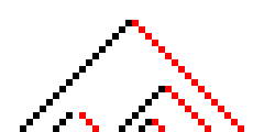
Figure 5. Particle system for the traffic automaton.
Proof.

We consider the chequerboard SFT Σ={∞(01)∞,∞(10)∞}\Sigma=\{\mathstrut^{\infty}(01)^{\infty},\mathstrut^{\infty}(10)^{\infty}\}, which is 22-periodic and F184F_{184}-invariant. Using the dislocation formalism, we define the phases φ(∞(01)∞)=0\varphi(\mathstrut^{\infty}(01)^{\infty})=0 and φ(∞(10)∞)=1\varphi(\mathstrut^{\infty}(10)^{\infty})=1, obtaining a set of particles defined by their local phases {p01,p10}\{p_{01},p_{10}\}. The corresponding morphism of order r=2r=2 is defined by the local rule:

00→p0111→p10otherwise→0.\begin{array}[]{ccc}00&\to&p_{01}\\ 11&\to&p_{10}\\ \mbox{otherwise}&\to&0\end{array}.

Indeed, consider x∈𝒜ℤx\in\mathcal{A}^{\mathbb{Z}} with a defect x01=00x_{01}=00. The phase of the 00 in position 00 is 00 and the phase of the 00 in position 11 is 11, so this corresponds to a particle p01p_{01}. Changing the position of the defect would not change the particle since the local phase would be modified accordingly.

The update function is defined in the intuitive manner: with p01p_{01} evolving at speed +1+1 and p10p_{10} at speed −1-1 and both particles being sent to ∅\emptyset in case of collision.

∀x∈𝒜ℤ,∀k∈ℤ,ϕ⁡(x,k)={{k−1}if ​π​(x)k=p10​ and ​π​(x)k−2≠p01{k+1}if ​π​(x)k=p01​ and ​π​(x)k+2≠p10∅OPENotherwise (and in particular if ​π​(x)k=0)\forall x\in\mathcal{A}^{\mathbb{Z}},\forall k\in\mathbb{Z},\phi(x,k)=\left\{\begin{array}[]{cl}\{k-1\}&\mbox{if }\pi(x)_{k}=p_{10}\mbox{ and }\pi(x)_{k-2}\neq p_{01}\\ \{k+1\}&\mbox{if }\pi(x)_{k}=p_{01}\mbox{ and }\pi(x)_{k+2}\neq p_{10}\\ \emptyset&\text{otherwise (and in particular if }\pi(x)_{k}=0)\end{array}\right.

We now check that the particle system satisfies all necessary conditions. To do that, one should verify that the update function is defined properly, that is:

∀x∈𝒜ℤ,∀k∈ℤ,π​(F⁡(x))k−1=p10\displaystyle\forall x\in\mathcal{A}^{\mathbb{Z}},\ \forall k\in\mathbb{Z},\ \pi(F(x))_{k-1}=p_{10} ⇔F​(x){k−1,k}=11\displaystyle\Leftrightarrow F(x)_{\{k-1,k\}}=11
⇔x[k−2,k+1]∈{1011,0111,1111}\displaystyle\Leftrightarrow x_{[k-2,k+1]}\in\{1011,0111,1111\}
⇔π​(x)k=p10​ and ​π​(x)k+2≠p01,\displaystyle\Leftrightarrow\pi(x)_{k}=p_{10}\mbox{ and }\pi(x)_{k+2}\neq p_{01},

and similarly for p01p_{01}. This type of proof can become tedious due to the high number of cases but can be automated by straightforward enumeration, here of all patterns of length 44. The different conditions follow from this property:

Locality:

Obvious by definition of ϕ\phi.

Redistribution:

The claim can be restated as π​(F⁡(x))k+1=p10⇔π​(x)k=p10\pi(F(x))_{k+1}=p_{10}\Leftrightarrow\pi(x)_{k}=p_{10} and ϕ⁡(x,k)={k+1}\phi(x,k)=\{k+1\}, and similarly for p01p_{01}. The first condition follows. Since ϕ⁡(x,k)=∅\phi(x,k)=\emptyset when k∉Part​(x)k\notin\textrm{Part}(x) by definition of ϕ\phi, the second condition follows.

Disjunction:

For k<k′k<k^{\prime}, to have ϕ⁡(x,k)>ϕ⁡(x,k′)\phi(x,k)>\phi(x,k^{\prime}), the only way would be to have π​(x)k′=p01\pi(x)_{k^{\prime}}=p_{01}, π​(x)k=p10\pi(x)_{k}=p_{10} and k′=k+1k^{\prime}=k+1. In that case, by definition, ϕ⁡(x,k)=ϕ⁡(x,k′)=∅\phi(x,k)=\phi(x,k^{\prime})=\emptyset.

Coalescence and speeds:

Obvious by definition of ϕ\phi.

Therefore we can apply Corollary 1 and only one type of particle remains in Λμ​(F184)\Lambda_{\mu}(F_{184}).

Furthermore, since the collisions are of the form p01+p10→∅p_{01}+p_{10}\to\emptyset, it is clear that for all x∈𝒜ℤx\in\mathcal{A}^{\mathbb{Z}}, 𝒟p01​(F184​(x))−𝒟p01​(x)=𝒟p10​(F184​(x))−𝒟p10​(x)\mathcal{D}_{p_{01}}(F_{184}(x))-\mathcal{D}_{p_{01}}(x)=\mathcal{D}_{p_{10}}(F_{184}(x))-\mathcal{D}_{p_{10}}(x). Therefore, which particle remains is decided according to whether μ⁡([00])>μ⁡([11])\mu([00])>\mu([11]) or the opposite, both particles disappearing in case of equality. The third case follows from the fact that if 00,11∉ℒ⁡(Λμ​(F184))00,11\notin\mathcal{L}(\Lambda_{\mu}(F_{184})), then Λμ(F184)={∞01∞,∞10∞}\Lambda_{\mu}(F_{184})=\{\mathstrut^{\infty}01^{\infty},\mathstrut^{\infty}10^{\infty}\} which support a unique measure δ01^\widehat{\delta_{01}}. ∎

2.6.2. nn-state cyclic automaton

The nn-state cyclic automaton CnC_{n} is a cellular automaton defined on the alphabet 𝒜=ℤ/n​ℤ\mathcal{A}=\mathbb{Z}/n\mathbb{Z} by the local rule

cn​(xi−1,xi,xi+1)={xi+1if ​xi−1=xi+1​ or ​xi+1=xi+1;xiotherwise.c_{n}(x_{i-1},x_{i},x_{i+1})=\left\{\begin{array}[]{ll}x_{i}+1&\mbox{if }x_{i-1}=x_{i}+1\mbox{ or }x_{i+1}=x_{i}+1;\\ x_{i}&\mbox{otherwise.}\end{array}\right.

See Figure 1 for an example of space-time diagram.

This automaton was introduced by [Fis90b]. In this paper, the author shows that for all Bernoulli measure μ\mu, the set [i]0[i]_{0} (for i∈𝒜i\in\mathcal{A}) is a μ\mu-attractor iff n≥5n\geq 5: that is, μ({x∈𝒜ℤ:∃T∈ℕ,∀t≥T,Ftx∈[i]})>0\mu(\{x\in\mathcal{A}^{\mathbb{Z}}\ :\ \exists T\in\mathbb{N},\forall t\geq T,F^{t}x\in[i]\})>0 for all ii. Simulations starting from a random configuration suggest the following: for n=3n=3 or 44, monochromatic regions keep increasing in size; for n≥5n\geq 5, we observe the convergence to a fixed point where small regions are delimited by vertical lines. We use the main result to explain this observation.

Proposition 3.

Define:

u+\displaystyle u_{+} ={a​b∈𝒜2:(b−a)modn=+1};\displaystyle=\{ab\in\mathcal{A}^{2}:(b-a)\mod n=+1\};
u−\displaystyle u_{-} ={a​b∈𝒜2:(b−a)modn=−1};\displaystyle=\{ab\in\mathcal{A}^{2}:(b-a)\mod n=-1\};
u0\displaystyle u_{0} ={a​b∈𝒜2:(b−a)modn∉{−1,0,1}}.\displaystyle=\{ab\in\mathcal{A}^{2}:(b-a)\mod n\notin\{-1,0,1\}\}.

Then, for any measure μ∈ℳσ−erg​((ℤ/n​ℤ)ℤ)\mu\in\mathcal{M}_{\sigma-\textrm{erg}}((\mathbb{Z}/n\mathbb{Z})^{\mathbb{Z}}), only one of those three sets may intersect the language of Λμ​(Cn)\Lambda_{\mu}(C_{n}).

If furthermore μ\mu is a Bernoulli measure, then the persisting set can only be u0u_{0}.

Proof.

We consider the interface defects relatively to the decomposition Σ=⨆i∈𝒜Σi\Sigma=\bigsqcup_{i\in\mathcal{A}}\Sigma_{i}, where Σi={∞i∞}\Sigma_{i}=\{\mathstrut^{\infty}i^{\infty}\}. Σ\Sigma is a CnC_{n}-invariant SFT of radius r=2r=2, and defects are exactly transitions between colours. Thus we define 𝒫={pa​b:ab∈𝒜2,a≠b}\mathcal{P}=\{p_{ab}\ :\ ab\in\mathcal{A}^{2},a\neq b\}. One cell is enough to distinguish the domains (α=1\alpha=1) and we obtain a morphism π\pi of radius 22 defined by the local rule:

𝒜2→𝒫∪{0}a⋅a↦0a⋅b↦pa​bfor all ​a,b∈𝒜.\begin{array}[]{ccc}\mathcal{A}^{2}&\to&\mathcal{P}\cup\{0\}\\ a\cdot a&\mapsto&0\\ a\cdot b&\mapsto&p_{ab}\end{array}\quad\quad\mbox{for all }a,b\in\mathcal{A}.

Simulations suggest that pa​bp_{ab} evolves at constant speed +1+1 if a​b∈u+ab\in u_{+}, −1-1 if a​b∈u−ab\in u_{-} and 00 if a​b∈u0ab\in u_{0}. Particles progress at their assigned speed unless they meet another particle, in which case they interact according to the following chemistry:

  • •

    pa​b+pb​a→∅p_{ab}+p_{ba}\to\emptyset (if pa​bp_{ab} has speed +1);

  • •

    pa​b+pb​c→pa​cp_{ab}+p_{bc}\to p_{ac} (if pa​bp_{ab} and pb​cp_{bc} have speeds (+1,0)(+1,0) or (0,−1)(0,-1), only when n≥4n\geq 4), or

  • •

    pa​b+pb​c+pc​d→pa​dp_{ab}+p_{bc}+p_{cd}\to p_{ad}. (if pa​b,pb​cp_{ab},p_{bc} and pc​dp_{cd} have speeds +1,0,−1+1,0,-1 respectively, which is only possible for n=4n=4).

We group together the particles of same speed, writing p+={pa​b:a​b∈u+}p_{+}=\{p_{ab}\ :\ ab\in u_{+}\} and p−p_{-} and p0p_{0} similarly. Formally, for x∈𝒜ℤx\in\mathcal{A}^{\mathbb{Z}} and k∈ℤk\in\mathbb{Z} the update function is defined as:

ϕ⁡(x,k)={{k+1}if ​π​(x)k∈p+​ and ​{π​(x)k+1∈p+, orπ​(x)k+1∉𝒫​ and ​π​(x)k+2∉p−;{k−1}if ​π​(x)k∈p−​ and ​{π​(x)k−1∈p−, orπ​(x)k−1∉𝒫​ and ​π​(x)k−2∉p+;{k}if ​π​(x)k∈p0​ and ​π​(x)k+1∉p−​ and ​π​(x)k−1∉p+∅OPENotherwise (and in particular if ​π​(x)k=0).\phi(x,k)=\left\{\begin{array}[]{cl}\{k+1\}&\mbox{if }\pi(x)_{k}\in p_{+}\mbox{ and }\left\{\begin{array}[]{c}\pi(x)_{k+1}\in p_{+},\mbox{ or}\\ \pi(x)_{k+1}\notin\mathcal{P}\mbox{ and }\pi(x)_{k+2}\notin p_{-}\end{array}\right.;\\ \{k-1\}&\mbox{if }\pi(x)_{k}\in p_{-}\mbox{ and }\left\{\begin{array}[]{c}\pi(x)_{k-1}\in p_{-},\mbox{ or}\\ \pi(x)_{k-1}\notin\mathcal{P}\mbox{ and }\pi(x)_{k-2}\notin p_{+};\end{array}\right.\\ \{k\}&\mbox{if }\pi(x)_{k}\in p_{0}\mbox{ and }\pi(x)_{k+1}\notin p_{-}\mbox{ and }\pi(x)_{k-1}\notin p_{+}\\ \emptyset&\text{otherwise (and in particular if }\pi(x)_{k}=0).\end{array}\right.

As previously, we can check that the update function actually describes the dynamics of the particles. For all x∈ℤx\in\mathbb{Z}, we check that:

π​(F⁡(x))1∈p+\displaystyle\pi(F(x))_{1}\in p_{+} ⇔F​(x){1,2}=a​bwith ​a=b+1\displaystyle\Leftrightarrow F(x)_{\{1,2\}}=ab\quad\mbox{with }a=b+1
⇔x[0,3]∈{a​b​b​cwhere ​c≠aa​b​c​_where ​b=c+1d​a​c​bwhere ​d≠a+1​ and ​c=b−1\displaystyle\Leftrightarrow x_{[0,3]}\in\left\{\begin{array}[]{ll}abbc&\mbox{where }c\neq a\\ abc\_&\mbox{where }b=c+1\\ dacb&\mbox{where }d\neq a+1\mbox{ and }c=b-1\end{array}\right.
⇔{π​(x)0∈p+​ and ​π​(x)1∉𝒫​ and ​π​(x)2∉p−, or π​(x)1∈p0​ and ​π​(x)2∈p−​ with good chemistry ​(pa,a−2+pa−2,a−1→pa,a−1)\displaystyle\Leftrightarrow\left\{\begin{array}[]{ll}\pi(x)_{0}\in p_{+}\mbox{ and }\pi(x)_{1}\notin\mathcal{P}\mbox{ and }\pi(x)_{2}\notin p_{-},\mbox{ or }\\ \pi(x)_{1}\in p_{0}\mbox{ and }\pi(x)_{2}\in p_{-}\mbox{ with good chemistry }(p_{a,a-2}+p_{a-2,a-1}\to p_{a,a-1})\end{array}\right.

and so on for other particle types, from which we deduce the hypotheses of Corollary 1. Since [p+]=π⁡([u+])[p_{+}]=\pi([u_{+}]) and so on, we obtain the result.

If μ\mu is a Bernoulli measure: Consider the “mirror” map γ⁡((ak)k∈ℤ)=(a−k)k∈ℤ\gamma((a_{k})_{k\in\mathbb{Z}})=(a_{-k})_{k\in\mathbb{Z}}. γ\gamma is continuous, and thus measurable. We have μ⁡(γ⁡([u]))=μ⁡([u−1])=μ⁡([u])\mu(\gamma([u]))=\mu([u^{-1}])=\mu([u]), where (u1⋯un)−1=un⋯u1(u_{1}\cdots u_{n})^{-1}=u_{n}\cdots u_{1}. But π​(x)k∈p+⇔π​(γ⁡(x))−k∈p−\pi(x)_{k}\in p_{+}\Leftrightarrow\pi(\gamma(x))_{-k}\in p_{-}, and conversely; since F∘γ=γ∘FF\circ\gamma=\gamma\circ F, all measures F∗t​μF_{\ast}^{t}\mu are γ\gamma-invariant, and thus no particle in p+p_{+} or p−p_{-} can persist in ℒ​(π​(Λμ​(F)))\mathcal{L}(\pi(\Lambda_{\mu}(F))) (since otherwise, the symmetrical particle would persist too). ∎

For small values of nn or particular initial measures, this proposition can be refined in the following manner:

𝒏=𝟑\bm{n=3}:

p0p_{0} is empty. Given the combinatorics of collisions, where a particle in p+p_{+} can only disappear by colliding with a particle in p−p_{-}, we see that particles in p+p_{+} persist if and only if π∗​μ​([p+])>π∗​μ​([p−])\pi_{\ast}\mu([p_{+}])>\pi_{\ast}\mu([p_{-}]), and symmetrically. In the equality case (in particular, for any Bernoulli measure), no defect can persist in the μ\mu-limit set, which means that Λμ​(F)\Lambda_{\mu}(F) is a set of monochromatic configurations.

𝒏=𝟒\bm{n=4}:

If μ\mu is a Bernoulli measure, the result of [Fis90b] shows that [i]0[i]_{0} cannot be a μ\mu-attractor for any ii. In other words, for μ\mu-almost all xx, Ft​(x)F^{t}(x) does not converge, which means that particles in p+p_{+} or p−p_{-} cross the central column infinitely often (even though their probability to appear tends to 00). This could not happen if particles in p0p_{0} were persisting in π​(Λμ​(F))\pi(\Lambda_{\mu}(F)), and thus Λμ​(F)\Lambda_{\mu}(F) is a set of monochromatic configurations.

𝒏≥𝟓\bm{n\geq 5}:

If μ\mu is a nondegenerate Bernoulli measure, the result of [Fis90b] shows that [i]0[i]_{0} is a μ\mu-attractor for all ii. This means that some particles in p0p_{0} persist in π​(Λμ​(F))\pi(\Lambda_{\mu}(F)), and any configuration of Λμ​(F)\Lambda_{\mu}(F) contains only homogeneous regions separated by vertical lines.

For n=3n=3 or 44, since Λμ​(F)\Lambda_{\mu}(F) is a set of monochromatic configurations we deduce that the sequence (Fn​μ)n∈ℕ(F^{n}\mu)_{n\in\mathbb{N}} converges to a convex combination of Dirac measures. However this method does not give any insight as to the coefficient of each component. As shown in [HdM14], if μ\mu is a Bernoulli measure then

C3∗tμ⟶t→∞μ([2])δ0^+μ([0])δ1^+μ([1])δ2^.C_{3\ast}^{t}\mu\underset{t\to\infty}{\longrightarrow}\mu([2])\widehat{\delta_{0}}+\mu([0])\widehat{\delta_{1}}+\mu([1])\widehat{\delta_{2}}.

The problem is open for the 4-cyclic cellular automaton.

2.6.3. One-sided captive cellular automata

We consider the family of captive cellular automata F:𝒜ℤ→𝒜ℤF:\mathcal{A}^{\mathbb{Z}}\to\mathcal{A}^{\mathbb{Z}} of neighbourhood {0,1}\{0,1\}, which means that the local rule f:𝒜{0,1}→𝒜f:\mathcal{A}^{\{0,1\}}\to\mathcal{A} satisfies f⁡(a0​a1)∈{a0,a1}f(a_{0}a_{1})\in\{a_{0},a_{1}\}. See Figure 1 for an example of space-time diagram.

Proposition 4.

Let FF be a one-sided captive automaton and μ∈ℳσ−erg​(𝒜ℤ)\mu\in\mathcal{M}_{\sigma-\textrm{erg}}(\mathcal{A}^{\mathbb{Z}}). Define:

u+\displaystyle u_{+} ={ab∈𝒜2:a≠b,f(a,b)=a}\displaystyle=\{ab\in\mathcal{A}^{2}\ :\ a\neq b,\ f(a,b)=a\}
u−\displaystyle u_{-} ={ab∈𝒜2:a≠b,f(a,b)=b}\displaystyle=\{ab\in\mathcal{A}^{2}\ :\ a\neq b,\ f(a,b)=b\}

Then either u+∩ℒ⁡(Λμ​(F))=∅u_{+}\cap\mathcal{L}(\Lambda_{\mu}(F))=\emptyset or u−∩ℒ⁡(Λμ​(F))=∅u_{-}\cap\mathcal{L}(\Lambda_{\mu}(F))=\emptyset.

If moreover, for all a,b∈𝒜a,b\in\mathcal{A}, the local rule satisfies f⁡(a​b)=f⁡(b​a)f(ab)=f(ba) and μ\mu is a Bernoulli measure, then Λμ(F)⊆{∞a∞:a∈𝒜}\Lambda_{\mu}(F)\subseteq\{\mathstrut^{\infty}a^{\infty}\ :\ a\in\mathcal{A}\} (no particle remains).

Proof.

We consider the interface defects relative to the decomposition Σ=⨆i∈𝒜Σi\Sigma=\bigsqcup_{i\in\mathcal{A}}\Sigma_{i} where Σi={∞i∞}\Sigma_{i}=\{\mathstrut^{\infty}i^{\infty}\} and obtain the same particles 𝒫\mathcal{P} and morphism π\pi as the nn-state cyclic automata. pa​bp_{ab} evolve at speed −1-1 if f⁡(a,b)=bf(a,b)=b and 00 if f⁡(a,b)=af(a,b)=a, and we define p−1p_{-1} and p0p_{0} accordingly. The update function is defined as follows:

∀x∈𝒜ℤ,∀k∈ℤ,ϕ⁡(x,k)={{k}if ​π​(x)k∈p0​ and ​π​(x)k+1∉p−1{k−1}if ​π​(x)k∈p−1​ and ​π​(x)k−1∉p0∅otherwise\forall x\in\mathcal{A}^{\mathbb{Z}},\ \forall k\in\mathbb{Z},\ \phi(x,k)=\left\{\begin{array}[]{cl}\{k\}&\text{if }\pi(x)_{k}\in p_{0}\mbox{ and }\pi(x)_{k+1}\notin p_{-1}\\ \{k-1\}&\text{if }\pi(x)_{k}\in p_{-1}\mbox{ and }\pi(x)_{k-1}\notin p_{0}\\ \emptyset&\text{otherwise}\end{array}\right.

As in the two previous examples, we check by enumeration of cases that the update function describes the particle dynamics on all words of length 3:

∀x∈𝒜ℤ,∀k∈ℤ,F​(x)k∈p0\displaystyle\forall x\in\mathcal{A}^{\mathbb{Z}},\ \forall k\in\mathbb{Z},\ F(x)_{k}\in p_{0} ⇔F​(x)[k,k+1]=a​b​ where ​a≠b​ and ​f​(a,b)=a\displaystyle\Leftrightarrow F(x)_{[k,k+1]}=ab\mbox{ where }a\neq b\mbox{ and }f(a,b)=a
⇔x[k,k+1]=a​b​c​ where ​b=c​ or ​f​(b,c)=b\displaystyle\Leftrightarrow x_{[k,k+1]}=abc\mbox{ where }b=c\mbox{ or }f(b,c)=b
⇔π​(x)k∈p0​ and ​π​(x)k+1∉p−1\displaystyle\Leftrightarrow\pi(x)_{k}\in p_{0}\mbox{ and }\pi(x)_{k+1}\notin p_{-1}

and deduce the properties of locality, redistribution, disjunction, coalescence and speed from there. The main result implies the theorem.

If μ\mu is a Bernoulli measure: Then μ\mu is invariant under the mirror map γ\gamma and F∘γ=γ∘FF\circ\gamma=\gamma\circ F by hypothesis. As in the previous example, we conclude that no particle can persist in Λμ​(F)\Lambda_{\mu}(F). ∎

2.6.4. An automaton performing random walks

Let FF be defined on the alphabet 𝒜=(ℤ/2​ℤ)2\mathcal{A}=(\mathbb{Z}/2\mathbb{Z})^{2} on the neighbourhood {−2,…,2}\{-2,\dots,2\} by the local rule ff defined as follows:

f:(a−2,b−2),…,(a2,b2)↦(a−2+a2,c)​ where ​c=1​ if ​(a−1,b−1)=(1,1)​ or ​(a0,b0)=(0,1);0​ otherwise.f:(a_{-2},b_{-2}),\dots,(a_{2},b_{2})\mapsto(a_{-2}+a_{2},c)\mbox{ where }c=\begin{array}[]{l}1\mbox{ if }(a_{-1},b_{-1})=(1,1)\mbox{ or }(a_{0},b_{0})=(0,1);\\ 0\mbox{ otherwise.}\end{array}

Intuitively, the first layer performs addition mod 22 at distance 2, while the ones on the second layer behave as particles, moving right if the first layer contains a 1 and not moving if it contains a 0. Two colliding particles simply merge.

Refer to caption
Figure 6. Automaton performing random walks iterated on the uniform measure. ■\blacksquare is a particle, while the second layer is represented by □\square (0) or ■{\color[rgb]{0.5,0.5,0.5}\blacksquare} (1).
Proposition 5.

Let ν∈ℳσ−erg​((ℤ/2​ℤ)ℤ)\nu\in\mathcal{M}_{\sigma-\textrm{erg}}((\mathbb{Z}/2\mathbb{Z})^{\mathbb{Z}}) and μ=λ×ν\mu=\lambda\times\nu, where λ\lambda is the uniform measure on (ℤ/2​ℤ)ℤ(\mathbb{Z}/2\mathbb{Z})^{\mathbb{Z}}. Then F∗t​μ​⟶t→∞​λ×δ0^F_{\ast}^{t}\mu\underset{t\to\infty}{\longrightarrow}\lambda\times\widehat{\delta_{0}}.

Proof.

Pivato’s formalism is not necessary here. Consider the set of particles 𝒫={1}\mathcal{P}=\{1\} and the morphism π\pi that is the projection on the second layer. The update function is defined as:

∀x∈𝒜ℤ,∀k∈ℤ,ϕ⁡(x,k)={{k+1}if ​xk=(1,1);{k}if ​xk=(0,1);∅otherwise.\forall x\in\mathcal{A}^{\mathbb{Z}},\ \forall k\in\mathbb{Z},\ \phi(x,k)=\left\{\begin{array}[]{cc}\{k+1\}&\mbox{if }x_{k}=(1,1);\\ \{k\}&\mbox{if }x_{k}=(0,1);\\ \emptyset&\mbox{otherwise.}\end{array}\right.

Checking locality, redistribution, disjunction and coalescence is trivial here. Intuitively, each particle performs a random walk with independent steps and bias 12\frac{1}{2}. Thus Corollary 1 is not sufficient to conclude, and we need to use the general result of Theorem 1 by proving that {1}\{1\} clashes with itself.

Writing (akt,bkt)=Ft​(x)k(a_{k}^{t},b_{k}^{t})=F^{t}(x)_{k}, we have akt=∑n=0t(tn)​ak−2​t+4​n0mod2a_{k}^{t}=\sum_{n=0}^{t}\binom{t}{n}a_{k-2t+4n}^{0}\mod 2 by straightforward induction. Now take some configuration xx with a particle at position kk and consider ϕt​(x,k)\phi^{t}(x,k) the walk performed by the particle. First we prove that the particle performs a random walk as claimed above. We have:

ϕt+1​(x,k)−ϕt​(x,k)\displaystyle\phi^{t+1}(x,k)-\phi^{t}(x,k) =aϕt​(x,k)t\displaystyle=a^{t}_{\phi^{t}(x,k)}
=(∑n=0t(nt)​aϕt​(x,k)−2​t+4​n0)mod2\displaystyle=\left(\sum_{n=0}^{t}\binom{n}{t}a_{\phi^{t}(x,k)-2t+4n}^{0}\right)\mod 2
=(aϕt​(x,k)−2​t0+∑n=1t−1(nt)​aϕt​(x,k)−2​t+4​n0+aϕt​(x,k)+2​t0)mod2.\displaystyle=\left(a_{\phi^{t}(x,k)-2t}^{0}+\sum_{n=1}^{t-1}\binom{n}{t}a_{\phi^{t}(x,k)-2t+4n}^{0}+a_{\phi^{t}(x,k)+2t}^{0}\right)\mod 2.

In the last line, we isolated the leftmost and rightmost term. Since ϕt​(x,k)−2​t\phi^{t}(x,k)-2t is strictly decreasing and ϕt​(x,k)+2​t\phi^{t}(x,k)+2t is strictly increasing in tt, these terms do not appear in any ϕt′+1​(x,k)−ϕt′​(x,k)\phi^{t^{\prime}+1}(x,k)-\phi^{t^{\prime}}(x,k) for t′<tt^{\prime}<t. Therefore, if xx is drawn according to a Bernoulli measure, the value of aϕt​(x,k)±2​t0a_{\phi^{t}(x,k)\pm 2t}^{0} is independent of the value of all ϕt′+1​(x,k)−ϕt′​(x,k)\phi^{t^{\prime}+1}(x,k)-\phi^{t^{\prime}}(x,k) for t′<tt^{\prime}<t.

Formally, the behaviour of ϕt′​(x,k)\phi^{t^{\prime}}(x,k) (for t′≤tt^{\prime}\leq t) only depends on the random variables {an0:ϕt​(x,k)−2​t+1≤n≤ϕt​(x,k)+2​t−1}\{a_{n}^{0}\ :\ \phi^{t}(x,k)-2t+1\leq n\leq\phi^{t}(x,k)+2t-1\}. Let UU be any event in the sigma-algebra generated by these variables. Then we have:

μ⁡(ϕt+1​(x,k)−ϕt​(x,k)=0|U)=\displaystyle\mu\left(\phi^{t+1}(x,k)-\phi^{t}(x,k)=0\ |\ U\right)= μ⁡(aϕt​(x,k)−2​t0=0∧∑n=1t(nt)​aϕt​(x,k)−2​t+4​n0=0|U)\displaystyle\ \mu\left(a_{\phi^{t}(x,k)-2t}^{0}=0\wedge\sum_{n=1}^{t}\binom{n}{t}a_{\phi^{t}(x,k)-2t+4n}^{0}=0\ |\ U\right)
+μ⁡(aϕt​(x,k)−2​t0=1∧∑n=1t(nt)​aϕt​(x,k)−2​t+4​n0=1|U)\displaystyle+\mu\left(a_{\phi^{t}(x,k)-2t}^{0}=1\wedge\sum_{n=1}^{t}\binom{n}{t}a_{\phi^{t}(x,k)-2t+4n}^{0}=1\ |\ U\right)
=\displaystyle= μ⁡(aϕt​(x,k)−2​t0=0)⋅μ⁡(∑n=1t(nt)​aϕt​(x,k)−2​t+4​n0=0|U)\displaystyle\ \mu\left(a_{\phi^{t}(x,k)-2t}^{0}=0\right)\cdot\mu\left(\sum_{n=1}^{t}\binom{n}{t}a_{\phi^{t}(x,k)-2t+4n}^{0}=0\ |\ U\right)
+μ(aϕt​(x,k)−2​t0=1)⋅μ(∑n=1t(nt)aϕt​(x,k)−2​t+4​n0=1|U)\displaystyle+\mu\left(a_{\phi^{t}(x,k)-2t}^{0}=1\right)\cdot\mu\left(\sum_{n=1}^{t}\binom{n}{t}a_{\phi^{t}(x,k)-2t+4n}^{0}=1\ |\ U\right)
=\displaystyle= 12,\displaystyle\ \frac{1}{2},

where the second step is by independence of the leftmost term from all the other variables, and the third step uses μ⁡(aϕt​(x,k)−2​t0=0)=12\mu\left(a_{\phi^{t}(x,k)-2t}^{0}=0\right)=\frac{1}{2} since μ\mu is the uniform Bernoulli measure on the first component. We proved that (ϕt​(x,k))t∈ℕ(\phi^{t}(x,k))_{t\in\mathbb{N}} is a random walk with independent steps and bias 12\frac{1}{2}.

To apply the theorem, we now prove that the particle clashes with itself. Note that the random walks performed by different particles are not independent; however, we prove that they are pairwise independent.

Let k∈ℕk\in\mathbb{N}. We prove that, when xx is chosen according to μk\mu_{k} the conditional measure of μ\mu relative to the event π​(x)0=π​(x)k=1\pi(x)_{0}=\pi(x)_{k}=1, ϕt​(x,k)−ϕt​(x,0)\phi^{t}(x,k)-\phi^{t}(x,0) performs an unbiased and independent random walk with a “death condition” on 0 (particle collision). Consider the evolution of ϕt​(x,k)−ϕt​(x,0)\phi^{t}(x,k)-\phi^{t}(x,0) at each step:

δt​(x)\displaystyle\delta_{t}(x) =(ϕt+1​(x,k)−ϕt​(x,k))−(ϕt+1​(x,0)−ϕt​(x,0))\displaystyle=(\phi^{t+1}(x,k)-\phi^{t}(x,k))-(\phi^{t+1}(x,0)-\phi^{t}(x,0))
=(∑n=0t(nt)​aϕt​(x,k)−2​t+4​n0mod2)⏟T​1−(∑n=0t(nt)​aϕt​(x,0)−2​t+4​n0mod2)⏟T​2\displaystyle=\underbrace{\left(\sum_{n=0}^{t}\binom{n}{t}a_{\phi^{t}(x,k)-2t+4n}^{0}\mod 2\right)}_{T1}-\underbrace{\left(\sum_{n=0}^{t}\binom{n}{t}a_{\phi^{t}(x,0)-2t+4n}^{0}\mod 2\right)}_{T2}

Note that the leftmost term of T1 is independent from T2 and all the past values of ϕt+1​(x,k)−ϕt​(x,k)\phi^{t+1}(x,k)-\phi^{t}(x,k); similarly, the rightmost term of T2 is independent from T1 and all past values of ϕt+1​(x,0)−ϕt​(x,0)\phi^{t+1}(x,0)-\phi^{t}(x,0). By the same argument as above, T1 and T2 are each worth 00 or 11 with probability 12\frac{1}{2} independently of each other and of all values of δt′\delta_{t^{\prime}} for t′<tt^{\prime}<t. We conclude that δt\delta_{t} takes values −1,0,+1-1,0,+1 with probability 14,12,14\frac{1}{4},\frac{1}{2},\frac{1}{4} respectively independently of all values of δt′\delta_{t^{\prime}} for t′<tt^{\prime}<t.

Therefore ϕt​(x,k)−ϕt​(x,0)\phi^{t}(x,k)-\phi^{t}(x,0) performs an unbiased and independent random walk. This implies that μk({x:∀t,ϕt(x,k)>ϕt(x,0)})=0\mu_{k}(\{x\ :\ \forall t,\phi^{t}(x,k)>\phi^{t}(x,0)\})=0 (standard result in one-dimensional random walks). Since particles cannot cross, they almost surely end up being in interaction, and therefore {1}\{1\} clashes with itself μ\mu-almost surely. Applying the theorem, we find that no particle can remain in Λμ​(F)\Lambda_{\mu}(F).

More precisely, if we write πi\pi_{i} the morphism projecting on the ii-th coordinate, π2∗F∗tμ→δ0^\pi_{2\ast}F_{\ast}^{t}\mu\to\widehat{\delta_{0}}. Since the addition mod 2 automaton is surjective, it leaves the uniform measure invariant. Therefore π1∗F∗tμ=λ\pi_{1\ast}F_{\ast}^{t}\mu=\lambda, and we conclude that F∗t​μ→λ×δ0^F_{\ast}^{t}\mu\to\lambda\times\widehat{\delta_{0}}. ∎

2.7. Probabilistic cellular automata

2.7.1. Adaptation of our formalism for probabilistic cellular automata

This approach can be adapted to non-deterministic cellular automata, and in particular probabilistic cellular automata. We use here a generalised version of the standard definition.

Definition 5.

Let 𝒜\mathcal{A} be a finite alphabet and 𝒩⊂ℤ\mathcal{N}\subset\mathbb{Z}. We define a map that applies a bi-infinite sequence of local rules to a configuration componentwise:

Φ𝒩:(𝒜𝒜𝒩)ℤ×𝒜ℤ→𝒜ℤ((fi)i∈ℤ,(xi)i∈ℤ)↦(fi((xi+r)r∈𝒩)i∈ℤ.\Phi_{\mathcal{N}}:\begin{array}[]{rl}(\mathcal{A}^{\mathcal{A}^{\mathcal{N}}})^{\mathbb{Z}}\times\mathcal{A}^{\mathbb{Z}}&\to\mathcal{A}^{\mathbb{Z}}\\ ((f_{i})_{i\in\mathbb{Z}},(x_{i})_{i\in\mathbb{Z}})&\mapsto(f_{i}((x_{i+r})_{r\in\mathcal{N}})_{i\in\mathbb{Z}}.\end{array}
Definition 6 (Generalised probabilistic cellular automata).

A generalised probabilistic cellular automaton F~\tilde{F} on the alphabet 𝒜\mathcal{A} with neighbourhood 𝒩\mathcal{N} is defined by a measure on bi-infinite sequence of local rules ν∈ℳσ​((𝒜𝒜𝒩)ℤ)\nu\in\mathcal{M}_{\sigma}((\mathcal{A}^{\mathcal{A}^{\mathcal{N}}})^{\mathbb{Z}}).

For a configuration x∈𝒜ℤx\in\mathcal{A}^{\mathbb{Z}}, F~:𝒜ℤ→ℳσ​(𝒜ℤ)\tilde{F}:\mathcal{A}^{\mathbb{Z}}\to\mathcal{M}_{\sigma}(\mathcal{A}^{\mathbb{Z}}) is then defined as:

For any Borel set ​U,F~​(x)​(U)=∫(𝒜𝒜𝒩)ℤ1U​(Φ𝒩​(f,x))​𝑑ν​(f).\mbox{For any Borel set }U,\ \tilde{F}(x)(U)=\int_{(\mathcal{A}^{\mathcal{A}^{\mathcal{N}}})^{\mathbb{Z}}}1_{U}(\Phi_{\mathcal{N}}(f,x))\mathrm{d}\nu(f).

A deterministic cellular automaton FF defined by a local rule ff corresponds in this formalism to a Dirac ν=δf^\nu=\widehat{\delta_{f}} (in which case the image measure is a Dirac on the image configuration), and usual probabilistic cellular automata correspond to the case where ν\nu is a Bernoulli measure; in other words, the local rule that applies at each coordinate is drawn independently among a finite set of local rules 𝒜𝒩→𝒜\mathcal{A}^{\mathcal{N}}\to\mathcal{A}.

Definition 7 (Action on the space of measures).

A generalised probabilistic cellular automaton defined by a measure ν∈ℳσ​((𝒜𝒜𝒩)ℤ)\nu\in\mathcal{M}_{\sigma}((\mathcal{A}^{\mathcal{A}^{\mathcal{N}}})^{\mathbb{Z}}) extends naturally to an action F~∗:ℳσ​(𝒜ℤ)→ℳσ​(𝒜ℤ)\tilde{F}_{\ast}:\mathcal{M}_{\sigma}(\mathcal{A}^{\mathbb{Z}})\to\mathcal{M}_{\sigma}(\mathcal{A}^{\mathbb{Z}}) by defining

F~∗​μ​(U)=∫𝒜ℤ∫(𝒜𝒜𝒩)ℤ1U​(Φ𝒩​(f,x))​𝑑ν​(f)​𝑑μ​(x).\tilde{F}_{\ast}\mu(U)=\int_{\mathcal{A}^{\mathbb{Z}}}\int_{(\mathcal{A}^{\mathcal{A}^{\mathcal{N}}})^{\mathbb{Z}}}1_{U}(\Phi_{\mathcal{N}}(f,x))\mathrm{d}\nu(f)\mathrm{d}\mu(x).

The μ\mu-limit measures set of F~\tilde{F}, 𝒱⁡(F~,μ)\mathcal{V}(\tilde{F},\mu), is the set of cluster points of the sequence (F~∗t​μ)t∈ℕ(\tilde{F}_{\ast}^{t}\mu)_{t\in\mathbb{N}}, and the μ\mu-limit set can be defined as

Λμ​(F~)=⋃η∈𝒱⁡(F~,μ)supp​η¯.\Lambda_{\mu}(\tilde{F})=\overline{\bigcup_{\eta\in\mathcal{V}(\tilde{F},\mu)}\mathrm{supp}\ \eta}.

The definitions of a particle system extend directly, except that the update function also depends on the choice of the local rules as well as on the configuration. Therefore we write ϕ⁡(x,n,(fi))\phi(x,n,(f_{i})) instead of ϕ⁡(x,n)\phi(x,n), where x∈𝒜ℤ,n∈ℤx\in\mathcal{A}^{\mathbb{Z}},n\in\mathbb{Z} and (fi)∈(𝒜𝒜𝒩)ℤ(f_{i})\in(\mathcal{A}^{\mathcal{A}^{\mathcal{N}}})^{\mathbb{Z}}, and the composition notation is simplified as follows (inductively):

ϕt​(x,n,(fk)0≤k<t)=⋃m∈ϕ⁡(x,n,f1)ϕt−1​(Φ𝒩​(f1,x),m,(fk)1≤k<t),\phi^{t}\left(x,n,(f^{k})_{0\leq k<t}\right)=\bigcup_{m\in\phi(x,n,f^{1})}\phi^{t-1}\left(\Phi_{\mathcal{N}}(f^{1},x),m,(f^{k})_{1\leq k<t}\right),

where each ft∈(𝒜𝒜𝒩)ℤf^{t}\in(\mathcal{A}^{\mathcal{A}^{\mathcal{N}}})^{\mathbb{Z}} is a bi-infinite sequence of local rules.

A particle system is said to be coalescent ν\nu-almost surely if the coalescence conditions hold for all x∈𝒜ℤx\in\mathcal{A}^{\mathbb{Z}} and ν\nu-almost every f∈(𝒜𝒜𝒩)ℤf\in(\mathcal{A}^{\mathcal{A}^{\mathcal{N}}})^{\mathbb{Z}}, and a particle p∈𝒫p\in\mathcal{P} has speed vv ν∞\nu^{\infty}-almost surely if the speed conditions hold for ν∞\nu^{\infty}-almost every sequence (ft)t∈ℕ(f^{t})_{t\in\mathbb{N}}, where ν∞\nu^{\infty} is the product measure (i.e. each ftf^{t} is drawn independently according to ν\nu). The clashing conditions are extended similarly.

Theorem 2 (Qualitative result for probabilistic automata).

Let F~:𝒜ℤ→ℳσ​(𝒜ℤ)\tilde{F}:\mathcal{A}^{\mathbb{Z}}\to\mathcal{M}_{\sigma}(\mathcal{A}^{\mathbb{Z}}) be a probabilistic cellular automaton defined by ν∈ℳσ​((𝒜𝒜𝒩)ℤ)\nu\in\mathcal{M}_{\sigma}((\mathcal{A}^{\mathcal{A}^{\mathcal{N}}})^{\mathbb{Z}}), μ\mu an initial σ\sigma-ergodic measure and (𝒫,π,ϕ)(\mathcal{P},\pi,\phi) a ν∞\nu^{\infty}-almost surely coalescent particle system for F~\tilde{F} where 𝒫\mathcal{P} can be partitioned into sets 𝒫1​…​𝒫n\mathcal{P}_{1}\dots\mathcal{P}_{n} such that, for any i<ji<j, 𝒫i\mathcal{P}_{i} clashes with 𝒫j\mathcal{P}_{j} μ,ν∞\mu,\nu^{\infty}-almost surely.

Then all particles appearing in the μ\mu-limit set belong to the same subset, i.e. there exists an ii such that

∀p∈𝒫,p∈ℒ⁡(π⁡(Λμ​(F)))⇒p∈𝒫i.\forall p\in\mathcal{P},\ p\in\mathcal{L}(\pi(\Lambda_{\mu}(F)))\Rightarrow p\in\mathcal{P}_{i}.

If furthermore there exists a jj such that 𝒫j\mathcal{P}_{j} clashes with itself μ,ν∞\mu,\nu^{\infty}-almost surely, then this set of particles does not appear in the μ\mu-limit set, i.e.

∀p∈𝒫,p∈ℒ⁡(π⁡(Λμ​(F)))⇒p∉𝒫j.\forall p\in\mathcal{P},\ p\in\mathcal{L}(\pi(\Lambda_{\mu}(F)))\Rightarrow p\notin\mathcal{P}_{j}.
Corollary 2 (Main result with speedy particles - probabilistic automata).

Let F~:𝒜ℤ→𝒜ℤ\tilde{F}:\mathcal{A}^{\mathbb{Z}}\to\mathcal{A}^{\mathbb{Z}} be a probabilistic cellular automaton defined by ν∈ℳσ​((𝒜𝒜𝒩)ℤ)\nu\in\mathcal{M}_{\sigma}((\mathcal{A}^{\mathcal{A}^{\mathcal{N}}})^{\mathbb{Z}}), μ\mu an initial σ\sigma-ergodic measure and (𝒫,π,ϕ)(\mathcal{P},\pi,\phi) a ν∞\nu^{\infty}-almost surely coalescent particle system for F~\tilde{F}. Assume that each particle p∈𝒫p\in\mathcal{P} has speed vp∈ℝv_{p}\in\mathbb{R} ν∞\nu^{\infty}-almost surely, then there is a speed v∈ℝv\in\mathbb{R} such that:

∀p∈𝒫,p∈ℒ⁡(π⁡(Λμ​(F)))⇒vp=v.\forall p\in\mathcal{P},\ p\in\mathcal{L}(\pi(\Lambda_{\mu}(F)))\Rightarrow v_{p}=v.

The proof of these statements are exactly the same as the proofs of Theorem 1 and Corollary 1, except that every statement in the proof holds ν∞\nu^{\infty}-almost surely.

This Theorem and Corollary can be applied for different probabilistic cellular automata, for example when we mix two one sided captive CA (see Figure 7). We are going to detail two examples from the literature and obtain new information about its limit measures (Section 2.7.2 and 2.7.3).

Refer to caption
Figure 7. Example of probabilistic cellular automata where the update of each cell is chosen between two one sided captive CA.

2.7.2. Example: Majority-traffic PCA

For any real p∈[0,1]p\in[0,1], consider the probabilistic automaton F~\tilde{F} on the alphabet {0,1}\{0,1\} defined on the neighbourhood 𝒩={−1,0,1}\mathcal{N}=\{-1,0,1\} by local rules drawn independently between the traffic rule (rule #184 defined in Section 2.6.1) with probability pp and the majority rule (rule #232 where F​(x)i=1F(x)_{i}=1 if and only if x−1+x0+x1≥2x_{-1}+x_{0}+x_{1}\geq 2) with probability 1−p1-p. This corresponds to the case where ν\nu is a Bernoulli measure.

This automaton was introduced by Fatès in [Fat13] as a candidate to solve the density classification problem.

Refer to caption Refer to caption Refer to caption
p=14p=\frac{1}{4} p=12p=\frac{1}{2} p=34p=\frac{3}{4}
Figure 8. Dynamics of the traffic-majority automaton iterated on the initial measure Ber⁡(35,25)\mathrm{Ber}(\frac{3}{5},\frac{2}{5}). Density classification is more efficient with pp close to 1.

In [BFMM13], the authors completely describe the invariant measures of this PCA. In the continuity of the rest of the article, we are interested in the convergence properties of all σ\sigma-ergodic initial measure. None of these two results imply the other.

Proposition 6 (Prop. 5.5 in [BFMM13]).

For any pp in [0,1][0,1], the set of F~\tilde{F}-invariant measures is the set of convex combinations of δ0^,δ1^\widehat{\delta_{0}},\widehat{\delta_{1}} and δ01^\widehat{\delta_{01}}.

Proposition 7.

Let μ∈ℳσ−erg​(𝒜ℤ)\mu\in\mathcal{M}_{\sigma-\textrm{erg}}(\mathcal{A}^{\mathbb{Z}}) and pp be a real in [0,1][0,1]. Then

Λμ(F~)⊂{∞0∞,∞1∞,∞(01)∞,∞(10)∞}.\Lambda_{\mu}(\tilde{F})\subset\{\mathstrut^{\infty}0^{\infty},\mathstrut^{\infty}1^{\infty},\mathstrut^{\infty}(01)^{\infty},\mathstrut^{\infty}(10)^{\infty}\}.

As a consequence, any μ\mu-limit measure of (F~∗t​μ)t∈ℕ(\tilde{F}^{t}_{\ast}\mu)_{t\in\mathbb{N}} is a convex combination of δ0^,δ1^\widehat{\delta_{0}},\widehat{\delta_{1}} and δ01^\widehat{\delta_{01}}.

Proof.

The cases p=0,1p=0,1 correspond to deterministic automata and can be treated easily.

The visual intuition suggests to consider interface defects according to the decomposition Σ0⊔Σ1⊔Σ2\Sigma_{0}\sqcup\Sigma_{1}\sqcup\Sigma_{2}, where Σ0={∞0∞}\Sigma_{0}=\{\mathstrut^{\infty}0^{\infty}\}, Σ1={∞1∞}\Sigma_{1}=\{\mathstrut^{\infty}1^{\infty}\} (monochromatic subshifts) and Σ2={∞(01)∞,∞(10)∞}\Sigma_{2}=\{\mathstrut^{\infty}(01)^{\infty},\mathstrut^{\infty}(10)^{\infty}\} (chequerboard subshift), since those SFTs are invariant under the action of both rules. The set of particles would be 𝒫={pi,j:i≠j∈{0,1,2}}\mathcal{P}=\{p_{i,j}:i\neq j\in\{0,1,2\}\}.

However, as Figure 9 shows, the particle p10p_{10} can “explode” and give birth to two particles p12p_{12} and p20p_{20}, contradicting the condition of coalescence. To solve this problem, we tweak the particle system by replacing each particle p10p_{10} by one particle p12p_{12} and one particle p20p_{20}.

[Uncaptioned image] “explosion”p12p_{12}p20p_{20}p02+p20=∅p_{02}+p_{20}=\emptysetp02+p21=p01p_{02}+p_{21}=p_{01}p01p_{01}
Figure 9. Fatès’ traffic-majority probabilistic automaton, with p=34p=\frac{3}{4}.

The corresponding morphism π\pi is defined on the neighbourhood {0,…,3}\{0,\dots,3\} by the local rule:

0011↦p01110​_↦p120010↦p02100​_↦p201011↦p21otherwise↦0\begin{array}[]{cccccc}0011&\mapsto&p_{01}&\quad 110\_&\mapsto&p_{12}\\ 0010&\mapsto&p_{02}&\quad 100\_&\mapsto&p_{20}\\ 1011&\mapsto&p_{21}&\quad\mbox{otherwise}&\mapsto&0\end{array}

where the wildcards _\_ can take both values.

Empirically, the particle behaviour without interactions is as follows. Regardless of the rule that is applied, p01,p02p_{01},p_{02} and p21p_{21} move at a constant speed 00, +1+1 and −1-1 respectively. A particle p12p_{12} moves at speed −1-1 if rule #​184\#184 is applied at its position and at speed +1+1 otherwise (independent random walk with bias 1−2​p1-2p), except if a particle p20p_{20} prevents its movement to the right, in which case it does not move. The particle p20p_{20} behaves symmetrically. As an abuse of notation, we denote for easier reading π​(x)0=p12−\pi(x)_{0}=p_{12}^{-} if π​(x)0=p12\pi(x)_{0}=p_{12} and fk=#​184f_{k}=\#184 and so on.

Particle interactions are of the form pi​j+pj​i→∅p_{ij}+p_{ji}\to\emptyset, pi​j+pj​k+pk​i→∅p_{ij}+p_{jk}+p_{ki}\to\emptyset, or pi​j+pj​k→pi​kp_{ij}+p_{jk}\to p_{ik}, although some of these can not happen. Interactions involve particles at distance at most 3.

Formally, we prove through exhaustive case enumeration of all patterns of length 7 and possible local rules that:

π​(F⁡(x))0=p01⟺\displaystyle\pi(F(x))_{0}=p_{01}\ \Longleftrightarrow (π​(x)0=p01​ and ​π​(x)−1≠p20+​ and ​π​(x)2≠p12−)\displaystyle\ (\pi(x)_{0}=p_{01}\mbox{ and }\pi(x)_{-1}\neq p_{20}^{+}\mbox{ and }\pi(x)_{2}\neq p_{12}^{-}) p01​ moves at speed 0\displaystyle p_{01}\textrm{ moves at speed $0$}
or ​(π​(x)−1=p02​ and ​π​(x)1=p21)\displaystyle\mbox{ or }(\pi(x)_{-1}=p_{02}\mbox{ and }\pi(x)_{1}=p_{21}) p02+p21→p01\displaystyle p_{02}+p_{21}\to p_{01}
π​(F⁡(x))0=p02⟺\displaystyle\pi(F(x))_{0}=p_{02}\ \Longleftrightarrow (π​(x)−1=p02​ and ​π​(x)1∉{p21,p20−})\displaystyle\ (\pi(x)_{-1}=p_{02}\mbox{ and }\pi(x)_{1}\notin\{p_{21},p_{20}^{-}\}) p02​ moves at speed +1\displaystyle p_{02}\textrm{ moves at speed $+1$}
or ​(π​(x)0=p01​ and ​π​(x)2=p12−​ and ​π​(x)−1≠p20+)\displaystyle\mbox{ or }(\pi(x)_{0}=p_{01}\mbox{ and }\pi(x)_{2}=p_{12}^{-}\mbox{ and }\pi(x)_{-1}\neq p_{20}^{+}) p01+p12→p02\displaystyle p_{01}+p_{12}\to p_{02}
π​(F⁡(x))0=p12⟺\displaystyle\pi(F(x))_{0}=p_{12}\ \Longleftrightarrow (π​(x)−1=p12+​ and ​π​(x)0∉{p21,p20−})\displaystyle\ (\pi(x)_{-1}=p_{12}^{+}\mbox{ and }\pi(x)_{0}\notin\{p_{21},p_{20}^{-}\}) p12+​ moves at speed +1\displaystyle p_{12}^{+}\textrm{ moves at speed $+1$}
or ​(π​(x)0=p12+​ and ​π​(x)1=p20−)\displaystyle\mbox{ or }(\pi(x)_{0}=p_{12}^{+}\mbox{ and }\pi(x)_{1}=p_{20}^{-}) p12+​ is blocked\displaystyle p_{12}^{+}\textrm{ is blocked}
or ​(π​(x)1=p12−​ and ​π​(x)−1≠p01)\displaystyle\mbox{ or }(\pi(x)_{1}=p_{12}^{-}\mbox{ and }\pi(x)_{-1}\neq p_{01}) p12−​ moves at speed −1\displaystyle p_{12}^{-}\textrm{ moves at speed $-1$}
π​(F⁡(x))0=p20⟺\displaystyle\pi(F(x))_{0}=p_{20}\ \Longleftrightarrow (π​(x)−1=p20+​ and ​π​(x)1≠p01)\displaystyle\ (\pi(x)_{-1}=p_{20}^{+}\mbox{ and }\pi(x)_{1}\neq p_{01}) p20+​ moves at speed +1\displaystyle p_{20}^{+}\textrm{ moves at speed $+1$}
or ​(π​(x)0=p20−​ and ​π​(x)−1=p12+)\displaystyle\mbox{ or }(\pi(x)_{0}=p_{20}^{-}\mbox{ and }\pi(x)_{-1}=p_{12}^{+}) p20−​ is blocked\displaystyle p_{20}^{-}\textrm{ is blocked}
or ​(π​(x)1=p20−​ and ​π​(x)−1≠p02​ and ​π​(x)0=p12+)\displaystyle\mbox{ or }(\pi(x)_{1}=p_{20^{-}}\mbox{ and }\pi(x)_{-1}\neq p_{02}\mbox{ and }\pi(x)_{0}=p_{12}^{+}) p20−​ moves at speed −1\displaystyle p_{20}^{-}\textrm{ moves at speed $-1$}
π​(F⁡(x))0=p21⟺\displaystyle\pi(F(x))_{0}=p_{21}\ \Longleftrightarrow (π​(x)1=p21​ and ​π​(x)−1≠p02​ and ​π​(x)0≠p12+)\displaystyle\ (\pi(x)_{1}=p_{21}\mbox{ and }\pi(x)_{-1}\neq p_{02}\mbox{ and }\pi(x)_{0}\neq p_{12}^{+}) p21​ moves at speed −1\displaystyle p_{21}\textrm{ moves at speed $-1$}
or ​(π​(x)−1=p20+​ and ​π​(x)0=p01​ and ​π​(x)2≠p12−)\displaystyle\mbox{ or }(\pi(x)_{-1}=p_{20}^{+}\mbox{ and }\pi(x)_{0}=p_{01}\mbox{ and }\pi(x)_{2}\neq p_{12}^{-}) p20+p01→p21\displaystyle p_{20}+p_{01}\to p_{21}
π​(F⁡(x))0=0\displaystyle\pi(F(x))_{0}=0\qquad in all other cases (including other possible interactions)

Using this statement, it is straightforward though tedious to define formally the update function, and the various conditions of locality, disjunction, particle control, surjectivity and coalescence are proved similarly to the previous examples.

Assume p≥12p\geq\frac{1}{2}. We show that no particle can remain asymptotically by applying the main result on the sets (𝒫i)0≤i≤4(\mathcal{P}_{i})_{0\leq i\leq 4}: {p02}\{p_{02}\}, {p20}\{p_{20}\}, {p01}\{p_{01}\}, {p12}\{p_{12}\} and {p21}\{p_{21}\}. We need only to show the clashes relative to the second and fourth sets since all other clashes are consequences of the speed of these particles.

Let k∈ℕk\in\mathbb{N} and xx be such that π​(x)0=p02\pi(x)_{0}=p_{02} and π​(x)k∈{p12,p20}\pi(x)_{k}\in\{p_{12},p_{20}\}. Since p02p_{02} progresses at speed 1, the distance ϕt​(x,k)−ϕt​(x,0)\phi^{t}(x,k)-\phi^{t}(x,0) cannot increase, and it decreases by at least one with probability pp (respectively 1−p1-p). It is clear that the particles end up in interaction ν∞\nu^{\infty}-almost surely. Showing that p12p_{12} and p20p_{20} clash with p21p_{21} is symmetric.

Let xx be such that π​(x)0=p20\pi(x)_{0}=p_{20} and π​(x)k=p01\pi(x)_{k}=p_{01}. As long as there are no interactions, the distance ϕt​(x,k)−ϕt​(x,0)=−ϕt​(x,0)\phi^{t}(x,k)-\phi^{t}(x,0)=-\phi^{t}(x,0) performs an independent random walk of bias 2​p−12p-1, where a increasing step is sometimes replaced by a constant step. Such a random walk reaches 00 ν∞\nu^{\infty}-almost surely, which shows that the particles end up in interaction. The clashes between p01p_{01} and p12p_{12}, and between {p20}\{p_{20}\} and {p12}\{p_{12}\}, are proved in a similar manner. The same proof holds for p≤12p\leq\frac{1}{2} by exchanging the roles of p20p_{20} and p12p_{12}.

Applying Theorem 2, we conclude that only one particle pi​jp_{ij} can remain in the μ\mu-limit set. This result can be improved further: consider Vk={x∈Λμ​(F):π​(x)k=pi​j}V_{k}=\{x\in\Lambda_{\mu}(F):\pi(x)_{k}=p_{ij}\}. Configurations in VkV_{k} are of the form y⋅zy\cdot z, where y∈𝒜]−∞,k]y\in\mathcal{A}^{]-\infty,k]} is admissible for Σi\Sigma_{i} and z∈𝒜[k+1,+∞[z\in\mathcal{A}^{[k+1,+\infty[} is admissible for Σj\Sigma_{j}; in particular, they contain only one particle. For any measure η∈𝒱⁡(F~,μ)\eta\in\mathcal{V}(\tilde{F},\mu), η⁡(Vk)\eta(V_{k}) is independent from kk by σ\sigma-invariance, and η⁡(⋃kVk)=∑kη⁡(Vk)≤1\eta\left(\bigcup_{k}V_{k}\right)=\sum_{k}\eta(V_{k})\leq 1 by disjunction of the (Vk)k∈ℤ(V_{k})_{k\in\mathbb{Z}}. Consequently, η⁡(Vk)=0\eta(V_{k})=0, which means Vk∉supp⁡(η)V_{k}\notin\mathrm{supp}(\eta). We conclude that no particle remain in the μ\mu-limit set, or in other words, Λμ​(F)⊂Σ0∪Σ1∪Σ2\Lambda_{\mu}(F)\subset\Sigma_{0}\cup\Sigma_{1}\cup\Sigma_{2}. ∎

2.7.3. Example: Approximation of a line

A finite word of {0,1}∗\{0,1\}^{\ast} can be seen as a finite curve in ℤ2\mathbb{Z}^{2} taking its origin in (0,0)(0,0), moving right on a 00 and up on a 11. In [RR15], the authors introduce for any α∈ℚ∩[0,1]\alpha\in\mathbb{Q}\cap[0,1] a random process that, starting from a finite word w∈{0,1}∗w\in\{0,1\}^{\ast} whose frequency of symbols 11 is α\alpha, organises bits through local flips to obtain asymptotically a discrete segment of slope α\alpha.

We adapt these processes so that the flips are performed in parallel and on an infinite configuration, which gives a probabilistic cellular automaton for every slope α∈ℚ∩[0,1]\alpha\in\mathbb{Q}\cap[0,1]. We consider the action of this PCA on any initial σ\sigma-ergodic measure satisfying μ⁡([1])=α\mu([1])=\alpha. Using Theorem 2, we show that the sequence of measures converges towards the measure supported by a periodic configuration representing a discrete line of slope α\alpha. To simplify the presentation, we consider here that α=12\alpha=\frac{1}{2}; the method can be easily generalised to other slopes.

Define the following local rules:

  • •

    ii is the identity;

  • •

    r⁡(x−2,x−1,x0,x1)={x0 if ​x−2​x−1​x0​x1=0101​ or ​1010,x−1 otherwise;r(x_{-2},x_{-1},x_{0},x_{1})=\begin{cases}x_{0}&\text{ if }x_{-2}x_{-1}x_{0}x_{1}=0101\textrm{ or }1010,\\ x_{-1}&\text{ otherwise};\end{cases}

  • •

    ℓ⁡(x−1,x0,x1,x2)={x0 if ​x−1​x0​x1​x2=0101​ or ​1010,x1 otherwise.\ell(x_{-1},x_{0},x_{1},x_{2})=\begin{cases}x_{0}&\text{ if }x_{-1}x_{0}x_{1}x_{2}=0101\textrm{ or }1010,\\ x_{1}&\text{ otherwise}.\end{cases}

Let F~line\tilde{F}_{\textrm{line}} be a probabilistic cellular automaton (represented in Figure 10) defined by a σ\sigma-ergodic measure ν∈ℳσ​({g0,g1,g−1}ℤ)\nu\in\mathcal{M}_{\sigma}(\{g_{0},g_{1},g_{-1}\}^{\mathbb{Z}}) whose support is the subshift of finite type defined by the set of forbidden patterns

{i​r,ℓ​ℓ,ℓ​i,r​r,r​ℓ}.\{ir,\ \ell\ell,\ \ell i,\ rr,\ r\ell\}.

To put it more simply, any time the local rules in two consecutive cells are ℓ\ell and rr (which happens with positive probability), the probabilistic CA permutes these two letters, except if they are at the centre of a four-letter words 10101010 or 01010101. In any other situation, it acts as the identity.

Proposition 8.

Let μ∈ℳσ−erg​(𝒜ℤ)\mu\in\mathcal{M}_{\sigma-\textrm{erg}}(\mathcal{A}^{\mathbb{Z}}). Then:

μ⁡([00])>μ⁡([11])\displaystyle\mu([00])>\mu([11]) ⇒11∉Λμ​(F~line);\displaystyle\Rightarrow 11\notin\Lambda_{\mu}(\tilde{F}_{\textrm{line}});
μ⁡([00])<μ⁡([11])\displaystyle\mu([00])<\mu([11]) ⇒00∉Λμ​(F~line);\displaystyle\Rightarrow 00\notin\Lambda_{\mu}(\tilde{F}_{\textrm{line}});
μ⁡([00])=μ⁡([11])\displaystyle\mu([00])=\mu([11]) ⇒F~linet​μ→δ01^.\displaystyle\Rightarrow\tilde{F}_{\textrm{line}}^{t}\mu\to\widehat{\delta_{01}}.
Proof.

We consider the dislocation defects with regards to the chequerboard SFT Σ={∞(01)∞,∞(10)∞}\Sigma=\{\mathstrut^{\infty}(01)^{\infty},\mathstrut^{\infty}(10)^{\infty}\}. As in Section 2.6.1, we obtain the particles 11↦p0111\mapsto p_{01} and 00↦p1000\mapsto p_{10}. A particle p10p_{10} at position 00 moves at speed +2+2 if ℓ\ell is applied at position 11, at speed −2-2 if ℓ\ell is applied on position −1-1, and at speed 00 otherwise. The particle p01p_{01} is symmetrical and they annihilate on contact. Indeed, we check by straightforward case enumeration that:

π​(F~line​(x))0=p10\displaystyle\pi(\tilde{F}_{\textrm{line}}(x))_{0}=p_{10} ⇔F~line​(x)[0,1]=00\displaystyle\Leftrightarrow\tilde{F}_{\textrm{line}}(x)_{[0,1]}=00
⇔{x[0,1]=00 and ​f−1,x−1≠(ℓ,1),(f1,x2)≠(ℓ,1)x[−2,−1]=00 and ​f−1=ℓ,x1=0x[2,3]=00 and ​f1=ℓ,x0=0\displaystyle\Leftrightarrow\left\{\begin{array}[]{ll}x_{[0,1]}=00&\mbox{ and }f_{-1},\ x_{-1}\neq(\ell,1),\ (f_{1},x_{2})\neq(\ell,1)\\ x_{[-2,-1]}=00&\mbox{ and }f_{-1}=\ell,\ x_{1}=0\\ x_{[2,3]}=00&\mbox{ and }f_{1}=\ell,\ x_{0}=0\end{array}\right.
⇔{π​(x)0=p10 at speed ​0π​(x)−2=p10 at speed +2​ and ​π​(x)0≠p10π​(x)2=p10 at speed −2​ and ​π​(x)0≠p10,\displaystyle\Leftrightarrow\left\{\begin{array}[]{ll}\pi(x)_{0}=p_{10}&\mbox{ at speed }0\\ \pi(x)_{-2}=p_{10}&\mbox{ at speed }+2\mbox{ and }\pi(x)_{0}\neq p_{10}\\ \pi(x)_{2}=p_{10}&\mbox{ at speed }-2\mbox{ and }\pi(x)_{0}\neq p_{10}\end{array}\right.,

and similarly for p01p_{01}. From this we deduce the various hypotheses of theorem, including ν∞\nu^{\infty}-almost sure clashing which stems from the fact that particles perform random walks. The exact statement of the proposition follows through the same arguments as in Section 2.6.1; in particular, the third case corresponds to the discrete line of slope 12\frac{1}{2}.∎

Refer to caption
Figure 10. Example of a space-time diagram of F~line\tilde{F}_{\textrm{line}}, where ν\nu is the Markov measure maximising the entropy of the subshift of finite type defined by the forbidden patterns {f0​f−1,f1​f1,f1​f0,f−1​f−1,f−1​f1}\{f_{0}f_{-1},\ f_{1}f_{1},\ f_{1}f_{0},\ f_{-1}f_{-1},\ f_{-1}f_{1}\}.

3. Particle-based organisation: quantitative results

For some cellular automata with simple defect dynamics, the previous results can be refined with a quantitative approach: that is, to determine the asymptotic distribution of random variables related to the particles. In [KFD11], P. Kůrka, E. Formenti and A. Dennunzio considered Tn​(x)T_{n}(x), the entry time after time nn on the initial configuration xx, which is the waiting time before a particle appears in a given position after time nn. They restricted their study to a gliders automaton, which is a cellular automaton on 3 states: a background state and two particles evolving at speeds 0 and -1 that annihilate on contact. Thus, we have one entry time for each type of particle (Tn+​(x)T_{n}^{+}(x) and Tn−​(x)T_{n}^{-}(x)). When the initial configuration is drawn according to the Bernoulli measure of parameters (12,0,12)(\frac{1}{2},0,\frac{1}{2}), which means that each cell contains, independently, a particle of each type with probability 12\frac{1}{2}, they proved that:

∀α∈ℝ+,μ⁡(Tn−​(x)n≤α)​⟶n→∞​2π​arctan⁡α.\forall\alpha\in\mathbb{R}^{+},\penalty\ \mu\left(\frac{T_{n}^{-}(x)}{n}\leq\alpha\right)\underset{n\to\infty}{\longrightarrow}\frac{2}{\pi}\arctan\sqrt{\alpha}.

They also suggested to develop formal tools in order to be able to handle more complex automata, starting with the (−1,1)(-1,1) symmetric case.

In Section 3.2, we extend this result to allow arbitrary values for the particle speeds v−v_{-} and v+v_{+}, and relax the conditions on the initial measure to some mixing conditions. Then, when v−<0v_{-}<0 and v+≥0v_{+}\geq 0, we have:

∀α∈ℝ+,μ⁡(Tn−​(x)n≤α)​⟶n→∞​2π​arctan⁡(−v−​αv+−v−+v+​α),\forall\alpha\in\mathbb{R}^{+},\penalty\ \mu\left(\frac{T_{n}^{-}(x)}{n}\leq\alpha\right)\underset{n\to\infty}{\longrightarrow}\frac{2}{\pi}\arctan\left(\sqrt{\frac{-v_{-}\alpha}{v_{+}-v_{-}+v_{+}\alpha}}\right),

and symmetrically if we exchange ++ and −-. The proof relies on the fact that the behaviour of gliders automata can be characterised by some random walk process; this idea was introduced by V. Belitsky and P. Ferrari in [BF95] and was already used in [KM00] and [KFD11]. In our case, a particle appearing in a position corresponds to a minimum between two concurrent random walks. The new tool here is that under α\alpha-mixing conditions, we rescale this process and approximate it with a Brownian motion. Thus we obtain the explicit asymptotic distribution of entry times.

This method, consisting in associating a random walk to each gliders automata and studying this random walk using scale invariance, is not limited to this particular conjecture concerning entry times. Indeed, we see in the next two sections that it can be used to study the asymptotic behaviour of two other, arguably more natural, parameters: the particle density at time tt and the rate of convergence to the limit measure. However, we obtain only an upper bound instead of an explicit asymptotic distribution. There is no doubt this method can be adapted to other parameters in a similar way.

Furthermore, these results can be extended to other automata with similar behaviour, such as those in Figure 1, by factorising them onto a gliders automaton. This point is discussed in Section 3.6. This method is more difficult to generalise when there is birth of particle, even in a simple case such as the 44-cyclic cellular automaton.

3.1. Gliders automata and random walks

In this section we give the definition and the first properties of the class of gliders automata.

Definition 8 (Gliders automata).

Let v−<v+∈ℤv_{-}<v_{+}\in\mathbb{Z}. The (v−,v+)(v_{-},v_{+})-gliders automaton (or GA) GG is the cellular automaton of neighbourhood [−v+,−v−][-v_{+},-v_{-}] defined on the alphabet 𝒜={−1,0,+1}\mathcal{A}=\{-1,0,+1\} by the local rule:

f⁡(x−v+​…​x−v−)={+1if x−v+=+1 and ∀N≤−v−,∑n=−v++1Nxn≥0−1if x−v−=−1 and ∀N≥−v+,∑n=N−v−−1xn≤00otherwise.f(x_{-v_{+}}\dots x_{-v_{-}})=\left\{\begin{array}[]{cl}+1&\text{if }x_{-v_{+}}=+1\text{ and }\forall N\leq-v_{-},\sum_{n=-v_{+}+1}^{N}x_{n}\geq 0\\ -1&\text{if }x_{-v_{-}}=-1\text{ and }\forall N\geq-v_{+},\sum_{n=N}^{-v_{-}-1}x_{n}\leq 0\\ 0&\text{otherwise.}\end{array}\right.

In all the following, 𝒜={−1,0,+1}\mathcal{A}=\{-1,0,+1\} and the diagrams are represented with the convention □=0,■=+1,■=−1\square=0,\blacksquare=+1,{\color[rgb]{1,0,0}\blacksquare}=-1.

Refer to caption
Figure 11. Space-time diagram of the (−1,0)(-1,0)-gliders automaton on a random initial configuration.

Our results apply on automata with simple defects dynamics, namely, automata admitting a particle system with 𝒫={±1}\mathcal{P}=\{\pm 1\} and whose update function corresponds to a gliders automaton. We first prove our results for gliders automata before generalising them in Section 3.6. Let us introduce some tools that turn the study of the dynamics of a gliders automaton into the study of some random walk.

Definition 9 (Random walk associated with a configuration).

Let x∈{−1,0,1}ℤx\in\{-1,0,1\}^{\mathbb{Z}}. Define the partial sums SxS_{x} by:

Sx​(0)=0and∀k∈ℤ,Sx​(k+1)−Sx​(k)=xk.S_{x}(0)=0\quad\mbox{and}\quad\forall k\in\mathbb{Z},\ S_{x}(k+1)-S_{x}(k)=x_{k}.

We extend SxS_{x} to ℝ\mathbb{R} by piecewise linear interpolation: Sx​(t)=(⌈t⌉−t)​Sx​(⌊t⌋)+(t−⌊t⌋)​Sx​(⌈t⌉)S_{x}(t)=(\lceil t\rceil-t)S_{x}(\lfloor t\rfloor)+(t-\lfloor t\rfloor)S_{x}(\lceil t\rceil) for t∈ℝ\ℤt\in\mathbb{R}\backslash\mathbb{Z}. We also introduce the rescaled process Sxk:t↦Sx​(k​t)kS_{x}^{k}:t\mapsto\frac{S_{x}(kt)}{\sqrt{k}}.

This random walk is simpler to study than the space-time diagram of the gliders automaton, and actually contains the same amount of information, as shown by the following technical lemmas.

Definition 10.

Let f:ℝ→ℝf:\mathbb{R}\to\mathbb{R} and U⊂ℝU\subset\mathbb{R}. We define argmin 𝑈​f\underset{U}{\mbox{argmin }}f by:

∀t∈U,t=argmin 𝑈​f⟺∀t′∈U\{t},f⁡(t)<f⁡(t′).\forall t\in U,\ t=\underset{U}{\mbox{argmin }}f\Longleftrightarrow\forall t^{\prime}\in U\backslash\{t\},f(t)<f(t^{\prime}).

In other words, tt realises the strict minimum of ff on UU; this point is not always defined.

Lemma 2.

Let GG be the (v−,v+)(v_{-},v_{+})-gliders automaton. For all j∈ℤj\in\mathbb{Z} and n≥1n\geq 1,

j=argmin [j,j+n]​SG⁡(x)⟺j−v+=argmin [j−v+,j+n−v−]​Sx,\displaystyle j=\underset{[j,\ j+n]}{\mbox{argmin }}S_{G(x)}\Longleftrightarrow j-v_{+}=\underset{[j-v_{+},\ j+n-v_{-}]}{\mbox{argmin }}{S_{x}},
j=argmin [j−n,j]​SG⁡(x)⟺j−v−=argmin [j−n−v+,j−v−]​Sx.\displaystyle j=\underset{[j-n,\ j]}{\mbox{argmin }}S_{G(x)}\Longleftrightarrow j-v_{-}=\underset{[j-n-v_{+},\ j-v_{-}]}{\mbox{argmin }}S_{x}.
Proof.

We prove those equivalences by induction on nn. At each step, we prove only the first equivalence, the other one being symmetric.

Base case:
SG⁡(x)​(j)<SG⁡(x)​(j+1)\displaystyle S_{G(x)}(j)<S_{G(x)}(j+1) ⇔G​(x)j=+1\displaystyle\Leftrightarrow G(x)_{j}=+1
⇔xj−v+=+1 and ∀N≤−v−,∑t=−v++1Nxj+t≥0\displaystyle\Leftrightarrow x_{j-v_{+}}=+1\text{ and }\forall N\leq-v_{-},\sum_{t=-v_{+}+1}^{N}x_{j+t}\geq 0
⇔Sx​(j−v+)<min[j+1−v+,j+1−v−]​Sx.\displaystyle\Leftrightarrow S_{x}(j-v_{+})<\underset{[j+1-v_{+},\ j+1-v_{-}]}{\min}S_{x}.
Induction:

Assume both equivalences hold for some n≥1n\geq 1.

Suppose j=argmin [j,j+n+1]​SG⁡(x)j=\underset{[j,\ j+n+1]}{\mbox{argmin }}S_{G(x)}. In particular j=argmin [j,j+n]​SG⁡(x)j=\underset{[j,\ j+n]}{\mbox{argmin }}S_{G(x)}, and by induction hypothesis j−v+=argmin [j−v+,j+n−v−]​Sxj-v_{+}=\underset{[j-v_{+},\ j+n-v_{-}]}{\mbox{argmin }}{S_{x}}. We distinguish two cases:

  • •:

    if Sx​(j+n−v−+1)>Sx​(j−v+)S_{x}(j+n-v_{-}+1)>S_{x}(j-v_{+}), then j−v+=argmin [j−v+,j+n−v−+1]​Sxj-v_{+}=\underset{[j-v_{+},\ j+n-v_{-}+1]}{\mbox{argmin }}{S_{x}} and we conclude;

  • •:

    otherwise, this means that Sx​(j+n−v−+1)=Sx​(j−v+)S_{x}(j+n-v_{-}+1)=S_{x}(j-v_{+}) (the walk can decrease by at most one at each step), and thus

    j+n−v−+1=argmin [j−v++1,j+n−v−+1]​Sx.j+n-v_{-}+1=\underset{[j-v_{+}+1,\ j+n-v_{-}+1]}{\mbox{argmin }}{S_{x}}.

    By induction hypothesis,

    j+n+1=argmin [j+1,j+n+1]​SG⁡(x),j+n+1=\underset{[j+1,\ j+n+1]}{\mbox{argmin }}{S_{G(x)}},

    and in particular SG⁡(x)​(j+n+1)<SG⁡(x)​(j+1)S_{G(x)}(j+n+1)<S_{G(x)}(j+1). Therefore SG⁡(x)​(j+n+1)≤SG⁡(x)​(j)S_{G(x)}(j+n+1)\leq S_{G(x)}(j), a contradiction with the first assumption.

The converse is proved in a similar manner.

∎

Lemma 3.

Let GG be the (v−,v+)(v_{-},v_{+})-gliders automaton. For all j∈ℤj\in\mathbb{Z} and k≥0,k\geq 0,

Gt​(x)j=−1\displaystyle G^{t}(x)_{j}=-1 ⟺j−v−​t+1=argmin [j−v+​t,j−v−​t+1]​Sx\displaystyle\Longleftrightarrow j-v_{-}t+1=\underset{[j-v_{+}t,\ j-v_{-}t+1]}{\mbox{argmin }}S_{x}
Gt​(x)j=+1\displaystyle G^{t}(x)_{j}=+1 ⟺j−v+​t=argmin [j−v+​t,j−v−​t+1]​Sx.\displaystyle\Longleftrightarrow j-v_{+}t=\underset{[j-v_{+}t,\ j-v_{-}t+1]}{\mbox{argmin }}S_{x}.

This is illustrated in Figure 12.

Refer to caption
SxS_{x}j−k+1j-k+1j+kj+kaakkjjGk​(x)jG^{k}(x)_{j}
Figure 12. Illustration of Lemma 3. A strict minimum is reached on j−k+1j-k+1.
Proof.

By induction on tt, proving only the first equivalence at each step:

Base case (t=0)(t=0):

By definition of SxS_{x}, Sx​(j+1)<Sx​(j)⇔xj=−1S_{x}(j+1)<S_{x}(j)\Leftrightarrow x_{j}=-1.

Induction:

Assume that both equivalences hold for a given time tt. By applying the induction hypothesis on G⁡(x)G(x), Gt+1​(x)j=−1⇔j−v−​t+1=argmin [j−v+​t,j−v−​t+1]​SG⁡(x)G^{t+1}(x)_{j}=-1\Leftrightarrow j-v_{-}t+1=\underset{[j-v_{+}t,\ j-v_{-}t+1]}{\mbox{argmin }}S_{G(x)} and we conclude by applying Lemma 2.

∎

3.2. Entry times

The main result of Section 2 implies that, for any σ\sigma-ergodic initial measure μ\mu, ΛG​(μ)\Lambda_{G}(\mu) contains at most one kind of particle, which one depending on whether μ⁡([+1])>μ⁡([−1])\mu([+1])>\mu([-1]) or the opposite. When μ⁡([+1])=μ⁡([−1])\mu([+1])=\mu([-1]), ΛG​(μ)\Lambda_{G}(\mu) only contains the particle-free configuration 0∞∞\mathstrut{}^{\infty}0^{\infty}. In other words, G∗t​μ→δ0^G_{\ast}^{t}\mu\to\widehat{\delta_{0}}, which means that the probability of seeing a particle in any fixed finite window tends to 0 as t→∞t\to\infty.

Definition 11 (Entry times).

Let v−<0≤v+∈ℤv_{-}<0\leq v_{+}\in\mathbb{Z}, GG the (v−,v+)(v_{-},v_{+})-GA and x∈{−1,0,1}ℤx\in\{-1,0,1\}^{\mathbb{Z}}. We define:

Tn−(x)=min{k∈ℕ:∃i∈[0,|v−|−1],Gk+n(x)i=−1},T_{n}^{-}(x)=\min\{k\in\mathbb{N}\ :\ \exists i\in[0,|v_{-}|-1],\ G^{k+n}(x)_{i}=-1\},

with Tn−​(x)=∞T_{n}^{-}(x)=\infty if this set is empty. This is the entry time in the set {b∈{−1,0,1}ℤ:∃i∈[0,|v−|−1],bi=−1}\{b\in\{-1,0,1\}^{\mathbb{Z}}\ :\ \exists i\in[0,|v_{-}|-1],b_{i}=-1\} after time nn at position 0 starting from xx. We define Tn+​(x)T_{n}^{+}(x) in a symmetrical manner.

The size of the considered window is such that any particle “passing through” the column 0 appears in this window exactly once (See Figure 13). Of course entry times for particles of speed 0 make no sense. From now on, we only consider T−T^{-} for simplicity, all the results being valid for T+T^{+}.

Refer to caption
Tn−​(x)T_{n}^{-}(x)nnxx
Figure 13. An entry time for the (-3,1)-gliders automaton.

As a consequence of Birkhoff’s ergodic theorem, when μ⁡([−1])>μ⁡([+1])\mu([-1])>\mu([+1]), −1-1 particles persist μ\mu-almost surely and their density converges to a positive number. Therefore:

  • •

    μ⁡(Tn+​(x)=∞)​⟶n→∞​1\mu(T^{+}_{n}(x)=\infty)\underset{n\to\infty}{\longrightarrow}1;

  • •

    ∀α>0,μ⁡(Tn−​(x)n≤α)​⟶n→∞​1\forall\alpha>0,\mu\left(\frac{T_{n}^{-}(x)}{n}\leq\alpha\right)\underset{n\to\infty}{\longrightarrow}1,

and symmetrically. This is why we only consider the case μ⁡([−1])=μ⁡([+1])\mu([-1])=\mu([+1]). Kůrka and al. proved the following result:

Theorem 3 ([KFD11]).

For the (−1,0)(-1,0)-GA (“Asymmetric gliders”) with an initial measure μ=Ber⁡(12,0,12)\mu=\mathrm{Ber}\left(\frac{1}{2},0,\frac{1}{2}\right):

∀α>0,μ⁡(Tn−​(x)n≤α)​⟶n→∞​2π​arctan⁡α.\forall\alpha>0,\penalty\ \mu\left(\frac{T_{n}^{-}(x)}{n}\leq\alpha\right)\underset{n\to\infty}{\longrightarrow}\frac{2}{\pi}\arctan\sqrt{\alpha}.

In the same article, they conjectured that this result could be extended to any initial Bernoulli measure of parameters (p,1−2​p,p)(p,1-2p,p) for 0≤p≤120\leq p\leq\frac{1}{2} by replacing the right-hand term by 2π​arctan⁡2​p​α\frac{2}{\pi}\arctan\sqrt{2p\alpha}. We will prove that this conjecture is actually incorrect.

To state our result, we introduce two particular subclasses of ℳσ​(𝒜ℤ)\mathcal{M}_{\sigma}(\mathcal{A}^{\mathbb{Z}}). We introduce α\alpha-mixing coefficients of a measure μ∈ℳσ​(𝒜ℤ)\mu\in\mathcal{M}_{\sigma}(\mathcal{A}^{\mathbb{Z}}):

αμ(n)=sup{|μ(A∩B)−μ(A)μ(B)|:A∈𝔅]−∞,0],B∈𝔅[n,+∞[}.\alpha_{\mu}(n)=\sup\{|\mu(A\cap B)-\mu(A)\mu(B)|:A\in\mathcal{\mathfrak{B}}_{]-\infty,0]},B\in\mathcal{\mathfrak{B}}_{[n,+\infty[}\}.

where 𝔅[a,b]\mathfrak{B}_{[a,b]} is the Borel σ\sigma-algebra generated by the random variables (Xi)a≤i≤b(X_{i})_{a\leq i\leq b}.

Define:

  • •

    Ber=\mathrm{Ber}_{=} the set of Bernoulli measures on {−1,0,+1}ℤ\{-1,0,+1\}^{\mathbb{Z}} and parameters (p,1−2​p,p)(p,1-2p,p) for some 0<p≤120<p\leq\frac{1}{2};

  • •

    ℳ​i​x\mathcal{M}ix the set of measures μ∈ℳσ​({−1,0,+1}ℤ)\mu\in\mathcal{M}_{\sigma}(\{-1,0,+1\}^{\mathbb{Z}}) satisfying:

    • –

      ∫𝒜ℤx0​𝑑μ​(x)=0\int_{\mathcal{A}^{\mathbb{Z}}}x_{0}\ \mathrm{d}\mu(x)=0, i.e., μ⁡([−1])=μ⁡([+1])\mu([-1])=\mu([+1]);

    • –

      ∑k=0∞∫𝒜ℤx0⋅xk​𝑑μ​(x)\sum_{k=0}^{\infty}\int_{\mathcal{A}^{\mathbb{Z}}}x_{0}\cdot x_{k}\ \mathrm{d}\mu(x) converges absolutely to a real σμ2>0\sigma_{\mu}^{2}>0 (asymptotic variance);

    • –

      ∃ε>0,∑n≥0αμ​(n)14−ε<∞\exists\varepsilon>0,\sum_{n\geq 0}\alpha_{\mu}(n)^{\frac{1}{4}-\varepsilon}<\infty.

In particular, Ber=⊂ℳ​i​x\mathrm{Ber}_{=}\subset\mathcal{M}ix.

Theorem 4 (Quantitative result for entry time).

For any (v−,v+)(v_{-},v_{+})-GA with v−<0v_{-}<0 and v+≥0v_{+}\geq 0 and any initial measure μ∈ℳ​i​x\mu\in\mathcal{M}ix,

∀α>0,μ⁡(Tn−​(x)n≤α)​⟶n→∞​2π​arctan⁡(−v−​αv+−v−+v+​α).\forall\alpha>0,\penalty\ \mu\left(\frac{T_{n}^{-}(x)}{n}\leq\alpha\right)\underset{n\to\infty}{\longrightarrow}\frac{2}{\pi}\arctan\left(\sqrt{\frac{-v_{-}\alpha}{v_{+}-v_{-}+v_{+}\alpha}}\right).

Notice that this limit is independent from μ\mu (as long as μ∈ℳ​i​x\mu\in\mathcal{M}ix), disproving the conjecture when μ∈Ber=\mu\in\mathrm{Ber}_{=}.

3.3. Brownian motion and proof of the main result

The third hypothesis for ℳ​i​x\mathcal{M}ix is chosen so that the large-scale behaviour of the partial sums Sx​(t)S_{x}(t) can be approximated by a Brownian motion. This invariance principle is the core of our proofs. The first and second conditions ensure that the Brownian motion obtained this way have no bias and nonzero variance, respectively.

Definition 12 (Brownian motion).

A Brownian motion (or Wiener process) BB of mean 00 and variance σ2\sigma^{2} is a continuous time stochastic process taking values in ℝ\mathbb{R} such that:

  • –

    B⁡(0)=0B(0)=0,

  • –

    t↦B⁡(t)t\mapsto B(t) is almost surely continuous,

  • –

    B⁡(t2)−B⁡(t1)B(t_{2})-B(t_{1}) follow the normal law of mean 0 and variance (t2−t1)​σ2(t_{2}-t_{1})\sigma^{2};

  • –

    For t1<t2≤t1′<t2′t_{1}<t_{2}\leq t^{\prime}_{1}<t^{\prime}_{2}, increments B⁡(t2)−B⁡(t1)B(t_{2})-B(t_{1}) and B⁡(t2′)−B⁡(t1′)B(t^{\prime}_{2})-B(t^{\prime}_{1}) are independent.

See [MP10] for a general introduction to Brownian motion.

Proposition 9 (Rescaling property).

Let BB be a Brownian motion. Then, for any k>0k>0, t↦1k​B​(k​t)t\mapsto\frac{1}{\sqrt{k}}B(kt) is a Brownian motion with same mean and variance.

We now state some invariance principles, which consists in approximating rescaled random walks by Brownian motion. We use a strong version, which guarantees an almost sure convergence by considering a copy of the process in a richer probability space.

Theorem 5 ([ZC96], Corollary 9.3.1).

Let X=(Xi)i∈ℕX=(X_{i})_{i\in\mathbb{N}} be a family of random variables taking values in {−1,0,1}\{-1,0,1\}. We denote by αX​(n)\alpha_{X}(n) its α\alpha-mixing coefficients defined as:

αX(n)=sup{|P(A∩B)−P(A)P(B)|:t∈ℕ,A∈𝔅[0,t],B∈𝔅[t+n,+∞[},\alpha_{X}(n)=\sup\{|P(A\cap B)-P(A)P(B)|:t\in\mathbb{N},A\in\mathfrak{B}_{[0,t]},B\in\mathfrak{B}_{[t+n,+\infty[}\},

where again 𝔅[a,b]\mathfrak{B}_{[a,b]} is the sigma-algebra generated by (Xa,…,Xb)(X_{a},\dots,X_{b}).

Assume that:

  1. (1)

    ∀i,𝔼⁡(Xi)=0\forall i,\mathbb{E}(X_{i})=0;

  2. (2)

    1t​𝔼​(∑i,j=1⌊t⌋Xi⋅Xj)\frac{1}{t}\mathbb{E}\left(\sum_{i,j=1}^{\lfloor t\rfloor}X_{i}\cdot X_{j}\right) converges absolutely to some positive real σ2\sigma^{2};

  3. (3)

    ∃ε>0,∑n=1∞αX​(n)14+ε\exists\varepsilon>0,\sum_{n=1}^{\infty}\alpha_{X}(n)^{\frac{1}{4}+\varepsilon}.

Then we can define two processes X′=(Xi′)i∈ℕX^{\prime}=(X^{\prime}_{i})_{i\in\mathbb{N}} and BB on a richer probability space (Ω,ℙ)(\Omega,\mathbb{P}) such that:

  1. (1)

    XX and X′X^{\prime} have the same distribution;

  2. (2)

    BB is a Brownian motion of mean 0, variance σ2\sigma^{2};

  3. (3)

    for any ε>0\varepsilon>0,

    |∑i=1⌊t⌋Xi−B⁡(t)|=O⁡(t14+ε)ℙ​-almost surely.\left|\sum_{i=1}^{\lfloor t\rfloor}X_{i}-B(t)\right|=O\left(t^{\frac{1}{4}+\varepsilon}\right)\quad\mathbb{P}\mbox{-almost surely}.
Corollary 3.

Let μ∈ℳ​i​x\mu\in\mathcal{M}ix. For any fixed constants q<r∈ℝq<r\in\mathbb{R}, we can define a process X′=(Xi′)i∈ℤX^{\prime}=(X^{\prime}_{i})_{i\in\mathbb{Z}} and a family of processes (t↦Bn​(t))n∈ℕ(t\mapsto B_{n}(t))_{n\in\mathbb{N}} on a richer probability space (Ω,ℙ)(\Omega,\mathbb{P}) such that:

  1. (1)

    X′X^{\prime} has distribution μ\mu;

  2. (2)

    every BnB_{n} is a Brownian motion of mean 0 and variance σμ2>0\sigma_{\mu}^{2}>0;

  3. (3)

    for any ε>0\varepsilon>0, denoting by SX′S_{X^{\prime}} the piecewise linear function defined by SX′​(0)=0S_{X^{\prime}}(0)=0 and SX′​(k+1)−SX′​(k)=Xk′S_{X^{\prime}}(k+1)-S_{X^{\prime}}(k)=X^{\prime}_{k} for all k∈ℤk\in\mathbb{Z},

    ∀n∈ℕ,supt∈[q,r]|SX′​(n​t)n−Bn(t)|=O(n−14+ε)ℙ-almost surely.\forall n\in\mathbb{N},\sup_{t\in[q,r]}\left|\frac{S_{X^{\prime}}(nt)}{\sqrt{n}}-B_{n}(t)\right|=O\left(n^{-\frac{1}{4}+\varepsilon}\right)\quad\mathbb{P}\mbox{-almost surely}.
Proof.

We apply Theorem 5 on (Xi)i∈ℕ(X_{i})_{i\in\mathbb{N}}, where (Xi)i∈ℤ(X_{i})_{i\in\mathbb{Z}} is distributed according to μ\mu. Because μ\mu is σ\sigma-invariant, this is a stationary process. The first and third conditions are satisfied by definition of ℳ​i​x\mathcal{M}ix. For the second condition,

1n​∑0≤i,j≤n|𝔼⁡(Xi⋅Xj)|\displaystyle\frac{1}{n}\sum_{0\leq i,j\leq n}|\mathbb{E}(X_{i}\cdot X_{j})| =1n∑i=0n∑j=−in−i𝔼(|X0⋅Xj−i|)by stationarity\displaystyle=\frac{1}{n}\sum_{i=0}^{n}\sum_{j=-i}^{n-i}\mathbb{E}(|X_{0}\cdot X_{j-i}|)\qquad\textrm{by stationarity}
=∑i=−nnn+1−|i|n𝔼(|X0⋅Xi|)by reordering the sum\displaystyle=\sum_{i=-n}^{n}\frac{n+1-|i|}{n}\mathbb{E}(|X_{0}\cdot X_{i}|)\qquad\textrm{by reordering the sum}
∼n→∞2∑i=0n𝔼(|X0⋅Xi|)⟶n→∞2σμ2,\displaystyle\sim_{n\to\infty}2\sum_{i=0}^{n}\mathbb{E}(|X_{0}\cdot X_{i}|)\underset{n\to\infty}{\longrightarrow}2\sigma_{\mu}^{2},

by stationarity and the equivalence criterion for positive series. We obtain two processes X1=(Xi1)i∈ℕX^{1}=(X^{1}_{i})_{i\in\mathbb{N}} and B1B^{1} on a richer probability space (Ω,ℙ)(\Omega,\mathbb{P}) such that X1X^{1} has the same distribution as xx, B1B^{1} is a Brownian motion of mean 0, variance σμ2\sigma_{\mu}^{2}, and:

∀ε>0,|∑i=1⌊t⌋Xi1−B1(t)|=Ot→+∞(t14+ε)ℙ-almost surely.\forall\varepsilon>0,\left|\sum_{i=1}^{\lfloor t\rfloor}X^{1}_{i}-B^{1}(t)\right|=\underset{t\to+\infty}{O}\left(t^{\frac{1}{4}+\varepsilon}\right)\quad\mathbb{P}\mbox{-almost surely}.

Since the variables Xi1X^{1}_{i} take value in {−1,0,1}\{-1,0,1\}, we have for any tt |∑i=1⌊t⌋Xi1−SX1​(t)|<1\left|\sum_{i=1}^{\lfloor t\rfloor}X^{1}_{i}-S_{X^{1}}(t)\right|<1 (a staircase and piecewise linear function having the same values on ℕ\mathbb{N}). Therefore:

∀ε>0,|SX1(t)−B1(t)|=Ot→+∞(t14+ε)ℙ-almost surely.\forall\varepsilon>0,\left|S_{X^{1}}(t)-B^{1}(t)\right|=\underset{t\to+\infty}{O}\left(t^{\frac{1}{4}+\varepsilon}\right)\quad\mathbb{P}\mbox{-almost surely}.
∀ε>0,∀n∈ℕ,1n|SX1(tn)−B1(tn)|=On→∞(n−14+ϵ)⋅Ot→∞(|t|14+ϵ)ℙ-almost surely.\forall\varepsilon>0,\forall n\in\mathbb{N},\ \frac{1}{\sqrt{n}}\left|S_{X^{1}}(tn)-B^{1}(tn)\right|=\underset{n\to\infty}{O}\left(n^{-\frac{1}{4}+\epsilon}\right)\cdot\underset{t\to\infty}{O}\left(|t|^{\frac{1}{4}+\epsilon}\right)\quad\mathbb{P}\mbox{-almost surely}.

For any r∈ℝ+2r\in\mathbb{R}_{+}^{2}, taking the sup for t∈[0,r]t\in[0,r], we obtain:

∀ε>0,∀n∈ℕ,supt∈[0,r]|SX1​(t​n)n−B1​(t​n)n|=On→∞(n−14+ϵ)ℙ-almost surely.\forall\varepsilon>0,\forall n\in\mathbb{N},\ \sup_{t\in[0,r]}\left|\frac{S_{X^{1}}(tn)}{\sqrt{n}}-\frac{B^{1}(tn)}{\sqrt{n}}\right|=\underset{n\to\infty}{O}\left(n^{-\frac{1}{4}+\epsilon}\right)\quad\mathbb{P}\mbox{-almost surely}.

By rescaling property Bn1:t↦B1​(t​n)nB^{1}_{n}:t\mapsto\frac{B^{1}(tn)}{\sqrt{n}} is a Brownian motion of same mean and variance as B1B^{1}.

To extend the result to negative values, we apply the theorem again to (x−i−1)i∈ℕ(x_{-i-1})_{i\in\mathbb{N}}, obtaining a process X2X^{2} and a Brownian motion B2B^{2} satisfying the same asymptotic bound on t→−∞t\to-\infty. Joining both parts, we can see that the process X′=…​X−22,X−12,X01,X11​…X^{\prime}=\dots X^{2}_{-2},X^{2}_{-1},X^{1}_{0},X^{1}_{1}\dots have distribution μ\mu and Bn:t↦Bn1​(t)B_{n}:t\mapsto B_{n}^{1}(t) if t≥0t\geq 0, Bn2​(t)B_{n}^{2}(t) if t<0t<0 is a Brownian motion. ∎

For a survey of invariance principles under different assumptions, see [MR12].

We now prove the main theorem.

Proof of Theorem 4.

For any x∈{−1,0,1}ℤx\in\{-1,0,1\}^{\mathbb{Z}}, Lemma 3 applied on the column 0 gives:

Tn−​(x)\displaystyle T_{n}^{-}(x) =min{k∈ℕ|∃j∈[0,−v−[,Sx(−v−(n+k)+j+1)<min[−v+​(n+k)+j,−v−​(n+k)+j]Sx}\displaystyle=\min\left\{k\in\mathbb{N}\ |\ \exists j\in[0,-v_{-}[\penalty\ ,S_{x}(-v_{-}(n+k)+j+1)<\min_{[-v_{+}(n+k)+j,\ -v_{-}(n+k)+j]}S_{x}\right\}
=min{k∈ℕ|∃j∈[0,−v−[,Sx(−v−(n+k)+j+1)<min[−v+​(n+k)+j,−v−​n]Sx}\displaystyle=\min\left\{k\in\mathbb{N}\ |\ \exists j\in[0,-v_{-}[\penalty\ ,S_{x}(-v_{-}(n+k)+j+1)<\min_{[-v_{+}(n+k)+j,\ -v_{-}n]}S_{x}\right\}

Indeed, if (k,j)(k,j) is the smallest pair (in lexicographic order) such that Sx​(−v−​(n+k)+j+1)<min[−v+​(n+k)+j,−v−​n]⁡SxS_{x}(-v_{-}(n+k)+j+1)<\min_{[-v_{+}(n+k)+j,\ -v_{-}n]}S_{x}, then all pairs (k′,j′)<(k,j)(k^{\prime},j^{\prime})<(k,j) verify Sx​(−v−​(n+k′)+j′+1)≥min[−v+​(n+k)+j,−v−​n]⁡SxS_{x}(-v_{-}(n+k^{\prime})+j^{\prime}+1)\geq\min_{[-v_{+}(n+k)+j,\ -v_{-}n]}S_{x}, and therefore Sx​(−v−​(n+k)+j+1)<min[−v+​(n+k)+j,−v−​(n+k)+j]⁡SxS_{x}(-v_{-}(n+k)+j+1)<\min_{[-v_{+}(n+k)+j,\ -v_{-}(n+k)+j]}S_{x}.

Note that if this last condition is reached on k∈ℕk\in\mathbb{N}, since SxS_{x} is piecewise linear, it is attained for tt as soon as t>k−1t>k-1 and reciprocally. Thus:

Tn−(x)=inf{t≥0|∃j∈[0,−v−[,Sx(−v−(n+t)+j+2)<min[−v+​(n+t)+j+1,−v−​n]Sx}T_{n}^{-}(x)=\inf\left\{t\geq 0\ |\ \exists j\in[0,-v_{-}[\penalty\ ,S_{x}(-v_{-}(n+t)+j+2)<\min_{[-v_{+}(n+t)+j+1,-v_{-}n]}S_{x}\right\}

Replacing jj by 00 in this expression adds to the infimum a value comprised between 00 and −v−−1−v−\frac{-v_{-}-1}{-v_{-}} (remember v−<0v_{-}<0). Since the infimum is necessarily an integer, we compensate by taking the integer part:

Tn−​(x)\displaystyle T_{n}^{-}(x) =⌊inf{t≥0|Sx​(−v−​(n+t)+2)<min[−v+​(n+t)+1,−v−​n]⁡Sx}⌋\displaystyle=\left\lfloor\inf\left\{t\geq 0\ |\ S_{x}(-v_{-}(n+t)+2)<\min_{[-v_{+}(n+t)+1,-v_{-}n]}S_{x}\right\}\right\rfloor
=⌊inf{t≥0|Sxn​(−v−​(1+tn)+2n)<min[−v+​(1+tn)+1n,−v−]⁡Sxn}⌋\displaystyle=\left\lfloor\inf\left\{t\geq 0\ |\ S_{x}^{n}\left(-v_{-}\left(1+\frac{t}{n}\right)+\frac{2}{n}\right)<\min_{[-v_{+}(1+\frac{t}{n})+\frac{1}{n},-v_{-}]}S_{x}^{n}\right\}\right\rfloor
=⌊n⋅inf{t≥0|Sxn​(−v−​(1+t)+2n)<min[−v+​(1+t)+1n,−v−]⁡Sxn}⌋\displaystyle=\left\lfloor n\cdot\inf\left\{t\geq 0\ |\ S_{x}^{n}\left(-v_{-}(1+t)+\frac{2}{n}\right)<\min_{[-v_{+}(1+t)+\frac{1}{n},-v_{-}]}S_{x}^{n}\right\}\right\rfloor

where SxnS_{x}^{n} is the rescaled process t↦Sx​(n​t)nt\mapsto\frac{S_{x}(nt)}{\sqrt{n}}. Since SxS_{x} is 11-Lipschitz, SxnS_{x}^{n} is n\sqrt{n}-Lipschitz (i.e. |Skn​(t′)−Skn​(t)|≤n​|t′−t||S_{k}^{n}(t^{\prime})-S_{k}^{n}(t)|\leq\sqrt{n}|t^{\prime}-t|). Dividing the previous expression by nn, using the fact that t−1n≤⌊n​t⌋n≤tt-\frac{1}{n}\leq\frac{\lfloor nt\rfloor}{n}\leq t for all t,n∈ℝ×ℕt,n\in\mathbb{R}\times\mathbb{N}:

(1a) μ⁡(min[−v−,−v−​(1+α)]⁡Sxn+4n<min[−v+​(1+α),−v−]⁡Sxn)≤μ⁡(Tn−​(x)n≤α)\displaystyle\mu\left(\min_{[-v_{-},-v_{-}(1+\alpha)]}S_{x}^{n}+\frac{4}{\sqrt{n}}<\min_{[-v_{+}(1+\alpha),-v_{-}]}S_{x}^{n}\right)\leq\mu\left(\frac{T_{n}^{-}(x)}{n}\leq\alpha\right)
(1b) μ⁡(Tn−​(x)n≤α)≤μ⁡(min[−v−,−v−​(1+α)]⁡Sxn−3n<min[−v+​(1+α),−v−]⁡Sxn)\displaystyle\mu\left(\frac{T_{n}^{-}(x)}{n}\leq\alpha\right)\leq\mu\left(\min_{[-v_{-},-v_{-}(1+\alpha)]}S_{x}^{n}-\frac{3}{\sqrt{n}}<\min_{[-v_{+}(1+\alpha),-v_{-}]}S_{x}^{n}\right)

We now bound the left-hand term of (1a) from below and the right-hand term of (1b) from above. Using Corollary 3, we build a process X′X^{\prime} and a family of processes (Bn)n∈ℕ(B_{n})_{n\in\mathbb{N}} on a richer probability space (Ω,ℙ)(\Omega,\mathbb{P}) such that X′X^{\prime} is distributed according to μ\mu and the BnB_{n} are Brownian motions.

∀n∈ℕ,sup[−v+​(1+α),−v−​(1+α)]|SX′​(n​t)n−Bn(t)|=O(n−14+ε)ℙ-almost surely.\forall n\in\mathbb{N},\sup_{[-v_{+}(1+\alpha),-v_{-}(1+\alpha)]}\left|\frac{S_{X^{\prime}}(nt)}{\sqrt{n}}-B_{n}(t)\right|=O\left(n^{-\frac{1}{4}+\varepsilon}\right)\quad\mathbb{P}\mbox{-almost surely}.

By symmetry, Bnl​(t)=Bn​(−v−−t)−Bn​(−v−)B_{n}^{l}(t)=B_{n}(-v_{-}-t)-B_{n}(-v_{-}) and Bnr​(t)=Bn​(−v−+t)−Bn​(−v−)B_{n}^{r}(t)=B_{n}(-v_{-}+t)-B_{n}(-v_{-}) are two independent Brownian motions on [0,v−−v+​(1+α)][0,\ v_{-}-v_{+}(1+\alpha)] and [0,−v−​α][0,\ -v_{-}\alpha], respectively. Consequently, for any ε>0\varepsilon>0 and nn large enough:

μ⁡(min[−v−,−v−​(1+α)]⁡Sxn+ε<min[−v+​(1+α),−v−]⁡Sxn)\displaystyle\mu\left(\min_{[-v_{-},-v_{-}(1+\alpha)]}S_{x}^{n}+\varepsilon<\min_{[-v_{+}(1+\alpha),-v_{-}]}S_{x}^{n}\right) =ℙ⁡(min[−v−,−v−​(1+α)]⁡SX′n+ε<min[−v+​(1+α),−v−]⁡SX′n)\displaystyle=\mathbb{P}\left(\min_{[-v_{-},-v_{-}(1+\alpha)]}S_{X^{\prime}}^{n}+\varepsilon<\min_{[-v_{+}(1+\alpha),-v_{-}]}S_{X^{\prime}}^{n}\right)
≥ℙ⁡(min[−v−,−v−​(1+α)]⁡Bn+2​ε<min[−v+​(1+α),−v−]⁡Bn)\displaystyle\geq\mathbb{P}\left(\min_{[-v_{-},-v_{-}(1+\alpha)]}B_{n}+2\varepsilon<\min_{[-v_{+}(1+\alpha),-v_{-}]}B_{n}\right)
(2a) ≥ℙ⁡(min[0,−v−​α]⁡Bnl+2​ε<min[0,−v−+v+​(1+α)]⁡Bnr)\displaystyle\geq\mathbb{P}\left(\min_{[0,-v_{-}\alpha]}B_{n}^{l}+2\varepsilon<\min_{[0,-v_{-}+v_{+}(1+\alpha)]}B_{n}^{r}\right)

and a symmetrical upper bound for (1b):

(2b) μ⁡(min[−v−,−v−​(1+α)]⁡Sxn−ε<min[−v+​(1+α),−v−]⁡Sxn)\displaystyle\mu\left(\min_{[-v_{-},-v_{-}(1+\alpha)]}S_{x}^{n}-\varepsilon<\min_{[-v_{+}(1+\alpha),-v_{-}]}S_{x}^{n}\right) ≤ℙ⁡(min[0,−v−​α]⁡Bnl−2​ε<min[0,−v−+v+​(1+α)]⁡Bnr)\displaystyle\leq\mathbb{P}\left(\min_{[0,-v_{-}\alpha]}B_{n}^{l}-2\varepsilon<\min_{[0,-v_{-}+v_{+}(1+\alpha)]}B_{n}^{r}\right)

We now evaluate the right-hand expression in (2a).

For any Brownian motion BB and b>0b>0, we have by rescaling ℙ⁡(min[0,b]⁡B≥m)=ℙ⁡(min[0,1]⁡B≥mb)\displaystyle\mathbb{P}\left(\min_{[0,b]}B\geq m\right)=\mathbb{P}\left(\min_{[0,1]}B\geq\frac{m}{\sqrt{b}}\right). Furthermore, since BnlB_{n}^{l} and BnrB_{n}^{r} are independent, so are min[0,1]⁡Bxl\displaystyle\min_{[0,1]}B^{l}_{x} and min[0,1]⁡Bxr\displaystyle\min_{[0,1]}B^{r}_{x}. Denote by μm\mu_{m} the law of the minimum of a Brownian motion on [0,1][0,1], which is defined by the density function:

ℝ→ℝt↦e−t22 if ​t≤0,0 otherwise.(see [MP10]).\begin{array}[]{rcll}\mathbb{R}&\to&\mathbb{R}&\\ t&\mapsto&\frac{e^{-t^{2}}}{2}&\mbox{ if }t\leq 0,\\ &&0&\mbox{ otherwise.}\end{array}\quad\mbox{(see \cite[cite]{[\@@bibref{}{Morters-Peres}{}{}]}).}

This means that for any y,z>0y,z>0:

ℙ⁡(min[0,y]⁡Bnl<min[0,z]⁡Bnr)\displaystyle\mathbb{P}\left(\min_{[0,y]}B^{l}_{n}<\min_{[0,z]}B^{r}_{n}\right) =∫−∞0∫−∞01{y⋅m1≤z⋅m2}dμm(m2)dμm(m1)\displaystyle=\int_{-\infty}^{0}\int_{-\infty}^{0}1_{\{\sqrt{y}\cdot m_{1}\leq\sqrt{z}\cdot m_{2}\}}d\mu_{m}(m_{2})d\mu_{m}(m_{1})
=(i)​42​π​∫−∞0∫−∞z⋅m2ye−m122​e−m222​d​m1​d​m2\displaystyle\underset{(i)}{=}\frac{4}{2\pi}\int_{-\infty}^{0}\int_{-\infty}^{\frac{\sqrt{z}\cdot m_{2}}{\sqrt{y}}}e^{\frac{-m_{1}^{2}}{2}}e^{\frac{-m_{2}^{2}}{2}}dm_{1}dm_{2}
=(i​i)​2π​∫ππ+arctan⁡(yz)∫0+∞r​e−r22​𝑑r​𝑑θ\displaystyle\underset{(ii)}{=}\frac{2}{\pi}\int_{\pi}^{\pi+\arctan\left(\sqrt{\frac{y}{z}}\right)}\int_{0}^{+\infty}re^{\frac{-r^{2}}{2}}drd\theta
(3) =2π​arctan⁡(yz)\displaystyle=\frac{2}{\pi}\arctan\left(\sqrt{\frac{y}{z}}\right)

(i) by using the law of the minimum of a Brownian motion, (ii) by passing in polar variables. For ε>0\varepsilon>0, a similar calculation gives:

ℙ⁡(min[0,y]⁡Bnl<min[0,z]⁡Bnr)−ℙ⁡(min[0,y]⁡Bnl+2​ε<min[0,z]⁡Bnr)\displaystyle\mathbb{P}\left(\min_{[0,y]}B^{l}_{n}<\min_{[0,z]}B^{r}_{n}\right)-\mathbb{P}\left(\min_{[0,y]}B^{l}_{n}+2\varepsilon<\min_{[0,z]}B^{r}_{n}\right) ≤42​π​∫−∞0∫z⋅m2−2​εyz⋅m2ye−m122​e−m222​d​m1​d​m2\displaystyle\leq\frac{4}{2\pi}\int_{-\infty}^{0}\int_{\frac{\sqrt{z}\cdot m_{2}-2\varepsilon}{\sqrt{y}}}^{\frac{\sqrt{z}\cdot m_{2}}{\sqrt{y}}}e^{\frac{-m_{1}^{2}}{2}}e^{\frac{-m_{2}^{2}}{2}}dm_{1}dm_{2}
≤8​ε2​π​y​∫−∞0e−y​m222​z​e−m222​d​m2\displaystyle\leq\frac{8\varepsilon}{2\pi\sqrt{y}}\int_{-\infty}^{0}e^{\frac{-ym_{2}^{2}}{2z}}e^{\frac{-m_{2}^{2}}{2}}dm_{2}
(4) ⟶ε→0​0\displaystyle\underset{\varepsilon\to 0}{\longrightarrow}0

Using (3) and (4), we see that the right-hand term in (2a) converges to 2π​arctan⁡(−v−​αv+−v−+v+​α)\frac{2}{\pi}\arctan\left(\sqrt{\frac{-v_{-}\alpha}{v_{+}-v_{-}+v_{+}\alpha}}\right) as ε→0\varepsilon\to 0. The left-hand term in (2b) can be bounded from above by the same method. We apply this result to (1a) and (1b) by taking ε=3n\varepsilon=\frac{3}{\sqrt{n}} (resp. 4n\frac{4}{\sqrt{n}}), and the theorem follows. ∎

3.4. Particle density

Definition 13 (Particle density in a configuration).

The −1-1 particle density in x∈{−1,0,1}ℤx\in\{-1,0,1\}^{\mathbb{Z}} is defined as d−​(x)=Freq​(−1,x)d_{-}(x)=\textrm{Freq}(-1,x). d+​(x)d_{+}(x) is defined in a symmetrical manner.

In all the following, any result on d−d_{-} also holds for d+d_{+} by symmetry.

Theorem 6 (Decrease rate of the particle density).

Let GG be a (v−,v+)(v_{-},v_{+})-GA with initial measure μ∈ℳ​i​x\mu\in\mathcal{M}ix. Then:

For μ-almost all ​x∈{−1,0,1}ℤ,∀ε>0,d−​(Gt​(x))=O⁡(t−14+ε)\textrm{For $\mu$-almost all }x\in\{-1,0,1\}^{\mathbb{Z}},\ \forall\varepsilon>0,\ d_{-}(G^{t}(x))=O\left(t^{-\frac{1}{4}+\varepsilon}\right)

If furthermore μ∈Ber=\mu\in\mathrm{Ber}_{=}:

For μ-almost all ​x∈{−1,0,1}ℤ,d−​(Gt​(x))∼t−12\textrm{For $\mu$-almost all }x\in\{-1,0,1\}^{\mathbb{Z}},\ d_{-}(G^{t}(x))\sim t^{-\frac{1}{2}}
Proof.

When μ∈ℳ​i​x\mu\in\mathcal{M}ix, it is in particular σ\sigma-ergodic, and so are its images G∗t​μG_{\ast}^{t}\mu. By Birkhoff’s ergodic theorem, one has d−​(Gt​(x))=G∗t​μ​([−1])=μ⁡(Gt​(x)0=−1)d_{-}(G^{t}(x))=G_{\ast}^{t}\mu([-1])=\mu(G^{t}(x)_{0}=-1) for μ\mu-almost all x∈{−1,0,1}ℤx\in\{-1,0,1\}^{\mathbb{Z}}.

We first prove the theorem when GG is the (−1,0)(-1,0)-gliders automaton. By Lemma 3,

μ⁡(Gt​(x)0=−1)=μ⁡(Sx​(t+1)<min[0,t]⁡Sx).\mu(G^{t}(x)_{0}=-1)=\mu\left(S_{x}(t+1)<\min_{[0,t]}S_{x}\right).
Equivalence (μ∈Ber=\mu\in\mathrm{Ber}_{=}):

By symmetry,

μ⁡(Sx​(t+1)<min[0,t]⁡Sx)=μ⁡(Sx​(0)<min[1,t+1]⁡Sx),\mu\left(S_{x}(t+1)<\min_{[0,t]}S_{x}\right)=\mu\left(S_{x}(0)<\min_{[1,t+1]}S_{x}\right),

which is the probability that the random walk starting from 0 remains strictly positive during tt steps, also known as its probability of survival. According to [Red01], when the random walk is symmetric and the steps are independent, we have the equivalence μ⁡(Gt​(x)0=−1)∼1t\mu(G^{t}(x)_{0}=-1)\sim\frac{1}{\sqrt{t}}.

Upper bound:
μ⁡(Sx​(t+1)<min[0,t]⁡Sx)≤μ⁡(Sxt+1​(1)=min[0,1]⁡Sxt+1).\mu\left(S_{x}(t+1)<\min_{[0,t]}S_{x}\right)\leq\mu\left(S_{x}^{t+1}(1)=\min_{[0,1]}S^{t+1}_{x}\right).

Using Corollary 3, we have:

μ⁡(Sxt+1​(1)=min[0,1]⁡Sxt+1)\displaystyle\mu\left(S_{x}^{t+1}(1)=\min_{[0,1]}S^{t+1}_{x}\right) =ℙ⁡(SX′t+1​(1)=min[0,1]⁡SX′t+1)\displaystyle=\mathbb{P}\left(S_{X^{\prime}}^{t+1}(1)=\min_{[0,1]}S^{t+1}_{X^{\prime}}\right)
≤ℙ⁡(Bt+1​(1)≤min[0,1]⁡Bt+1+Ct+1)\displaystyle\leq\mathbb{P}\left(B_{t+1}(1)\leq\min_{[0,1]}B_{t+1}+C_{t+1}\right)
≤ℙ⁡(Bt+1​(0)≤min[0,1]⁡Bt+1+Ct+1),\displaystyle\leq\mathbb{P}\left(B_{t+1}(0)\leq\min_{[0,1]}B_{t+1}+C_{t+1}\right),

where Ct+1=sup[0,1]|SX′t+1−Bt+1|=O⁡(t−14+ε)\displaystyle C_{t+1}=\sup_{[0,1]}\left|S_{X^{\prime}}^{t+1}-B_{t+1}\right|=O\left(t^{-\frac{1}{4}+\varepsilon}\right) ℙ\mathbb{P}-almost surely, and where the third line is obtained by symmetry of the Brownian motion.

Furthermore ℙ(min[0,1]Bt+1>−Ct+1)=∫−Ct+10e−x2/2dx≤Ct+1=O(t−14+ε)\displaystyle\mathbb{P}\left(\min_{[0,1]}B_{t+1}>-C_{t+1}\right)=\int_{-C_{t+1}}^{0}e^{-x^{2}/2}dx\leq C_{t+1}=O\left(t^{-\frac{1}{4}+\varepsilon}\right).

General case (any v−<v+v_{-}<v_{+}):

Let G′G^{\prime} be the (v−,v+)(v_{-},v_{+})-GA. Then

G′=σv+∘Gv+−v−.G^{\prime}=\sigma^{v_{+}}\circ G^{v_{+}-v_{-}}.

To conclude, it is enough to see that the particle density is σ\sigma-invariant and decreasing under the action of GG. ∎

3.5. Rate of convergence

In this section, we estimate the rate of convergence to the limit measure. For that we fix a distance on the space ℳσ​(𝒜ℤ)\mathcal{M}_{\sigma}(\mathcal{A}^{\mathbb{Z}}) of σ\sigma-invariant measures, which induces the weak∗ topology:

dℳ​(μ,ν)=∑n∈ℕ12n​maxu∈𝒜n​|μ⁡([u])−ν⁡([u])|.d_{\mathcal{M}}(\mu,\nu)=\sum_{n\in\mathbb{N}}\frac{1}{2^{n}}\max_{u\in\mathcal{A}^{n}}\left|\mu([u])-\nu([u])\right|.
Theorem 7 (Rate of convergence to the limit measure).

Let GG be the (v−,v+)(v_{-},v_{+})-GA with initial measure μ∈ℳ​i​x\mu\in\mathcal{M}ix. Then:

∀ε>0,dℳ(G∗tμ,δ0^)=O(t−1/4+ε)\forall\varepsilon>0,\ d_{\mathcal{M}}(G^{t}_{\ast}\mu,\widehat{\delta_{0}})=O\left(t^{-1/4+\varepsilon}\right)

If furthermore μ∈Ber=\mu\in\mathrm{Ber}_{=}:

dℳ(G∗tμ,δ0^)=Ω(t−1/2)d_{\mathcal{M}}(G^{t}_{\ast}\mu,\widehat{\delta_{0}})=\Omega\left(t^{-1/2}\right)
Proof.

We first prove the theorem when GG is the (−1,0)(-1,0)-gliders automaton. By defining 0ℓ∈𝒜ℓ0^{\ell}\in\mathcal{A}^{\ell} the word containing only zeroes, the distance can be rewritten:

∀t∈ℕ,dℳ​(G∗t​μ,δ0^)=∑ℓ=1∞12ℓ​G∗t​μ​(𝒜ℤ\[0ℓ]).\forall t\in\mathbb{N},d_{\mathcal{M}}(G_{\ast}^{t}\mu,\widehat{\delta_{0}})=\sum_{\ell=1}^{\infty}\frac{1}{2^{\ell}}G^{t}_{\ast}\mu\left(\mathcal{A}^{\mathbb{Z}}\backslash[0^{\ell}]\right).

Lower bound when μ∈Ber=\mu\in\mathrm{Ber}_{=}: dℳ​(G∗t​μ,δ0^)>G∗t​μ​(𝒜ℤ\[0])d_{\mathcal{M}}(G_{\ast}^{t}\mu,\widehat{\delta_{0}})>G^{t}_{\ast}\mu\left(\mathcal{A}^{\mathbb{Z}}\backslash[0]\right). We conclude with Theorem 6.

Upper bound: We give an upper bound for G∗tμ(𝒜ℤ\[0ℓ])=μ(∃0≤d≤ℓ,Gt(x)d=±1)G^{t}_{\ast}\mu(\mathcal{A}^{\mathbb{Z}}\backslash[0^{\ell}])=\mu(\exists 0\leq d\leq\ell,G^{t}(x)_{d}=\pm 1) for ℓ∈ℕ\ell\in\mathbb{N} and t∈ℕt\in\mathbb{N}. By Lemma 3,

∀d∈ℤ,Gt​(x)d=+1⇔Sx​(d)<min[d+1,d+t]⁡Sx.\forall d\in\mathbb{Z},\ G^{t}(x)_{d}=+1\Leftrightarrow S_{x}(d)<\min_{[d+1,d+t]}S_{x}.

Therefore:

G∗t​μ​(⋂d=0ℓ[+1]d)\displaystyle G^{t}_{\ast}\mu\left(\bigcap_{d=0}^{\ell}[+1]_{d}\right) ≤μ⁡(min[0,ℓ]⁡Sx<min[ℓ+1,t]⁡Sx)\displaystyle\leq\mu\left(\min_{[0,\ell]}S_{x}<\min_{[\ell+1,t]}S_{x}\right)
≤μ⁡(min[0,t]⁡Sx≥−ℓ)\displaystyle\leq\mu\left(\min_{[0,t]}S_{x}\geq-\ell\right)
≤μ⁡(min[0,1]⁡Sxt≥−ℓt)\displaystyle\leq\mu\left(\min_{[0,1]}S^{t}_{x}\geq-\frac{\ell}{\sqrt{t}}\right)

By Corollary 3, using the same notations as in the previous proofs:

G∗tμ(∃0≤d≤ℓ,xd=+1)\displaystyle G^{t}_{\ast}\mu\left(\exists 0\leq d\leq\ell,x_{d}=+1\right) ≤ℙ⁡(min[0,1]⁡SX′t≥−ℓt)\displaystyle\leq\mathbb{P}\left(\min_{[0,1]}S^{t}_{X^{\prime}}\geq-\frac{\ell}{\sqrt{t}}\right)
≤ℙ⁡(min[0,1]⁡Bt≥−ℓt−Ct) where ​Ct=O⁡(t−14+ε)\displaystyle\leq\mathbb{P}\left(\min_{[0,1]}B_{t}\geq-\frac{\ell}{\sqrt{t}}-C_{t}\right)\quad\quad\textrm{ where }C_{t}=O\left(t^{-\frac{1}{4}+\varepsilon}\right)
=O⁡(t−14+ε)\displaystyle=O\left(t^{-\frac{1}{4}+\varepsilon}\right)

for any ε>0\varepsilon>0, following the same calculations as in Section 3.4. The case of −1-1 particles is symmetrical, and we conclude.

General case:

Apply the same method as in the previous section, considering that dℳd_{\mathcal{M}} and all considered measures are σ\sigma-invariant and that any CA is Lipschitz w.r.t dℳd_{\mathcal{M}}. ∎

3.6. Extension to other cellular automata

Definition 14.

Let F1,F2F_{1},F_{2} be two CAs on 𝒜ℤ\mathcal{A}^{\mathbb{Z}} and ℬℤ\mathcal{B}^{\mathbb{Z}}, respectively. We say that F1F_{1} factorises onto F2F_{2} if there exists a factor π:𝒜ℤ→ℬℤ\pi:\mathcal{A}^{\mathbb{Z}}\to\mathcal{\mathcal{B}}^{\mathbb{Z}} such that π∘F1=F2∘π\pi\circ F_{1}=F_{2}\circ\pi.

In particular, if F2F_{2} admits a particle system (𝒫,π2,ϕ)(\mathcal{P},\pi_{2},\phi), then F1F_{1} admits a particle system with (𝒫,π∘π2,ϕ)(\mathcal{P},\pi\circ\pi_{2},\phi).

In this section, we extend the Theorems 4 and 6 to automata that factorise onto a gliders automaton, and discuss conditions for the extension of Theorem 7. In Section 2.5, we exhibited a general method to find such a factor using experimental intuition when such a factor is not obvious. In other words, we extend our results to automata that admit a particle system (𝒫,π,ϕ)(\mathcal{P},\pi,\phi), where 𝒫={−1,+1}\mathcal{P}=\{-1,+1\} and ϕ\phi updates the particle positions similarly to a gliders automaton.

In order to extend the theorem to such CAs, starting from an initial measure μ\mu, we must first ensure that π∗​μ∈ℳ​i​x\pi_{\ast}\mu\in\mathcal{M}ix. We show that the third condition in the definition of ℳ​i​x\mathcal{M}ix is invariant under morphism.

Proposition 10.

Let π:𝒜ℤ→ℬℤ\pi:\mathcal{A}^{\mathbb{Z}}\to\mathcal{B}^{\mathbb{Z}} be a morphism, μ∈ℳσ​(𝒜ℤ)\mu\in\mathcal{M}_{\sigma}(\mathcal{A}^{\mathbb{Z}}) and k>0k>0 any real such that ∑n≥0αμ​(n)k<∞\sum_{n\geq 0}\alpha_{\mu}(n)^{k}<\infty. Then, ∑n≥0απ∗​μ​(n)k<∞\sum_{n\geq 0}\alpha_{\pi_{\ast}\mu}(n)^{k}<\infty.

Proof.

We keep the notations from the definition of αμ​(n)\alpha_{\mu}(n). π\pi is defined by a local rule with neighbourhood 𝒩⊂[−r,r]\mathcal{N}\subset[-r,r] for some r>0r>0. Then, π−1𝔅]−∞,0]⊂𝔅]−∞,r]\pi^{-1}\mathfrak{B}_{]-\infty,0]}\subset\mathfrak{B}_{]-\infty,r]} and π−1𝔅[n,+∞[⊂𝔅[n−r,+∞[\pi^{-1}\mathfrak{B}_{[n,+\infty[}\subset\mathfrak{B}_{[n-r,+\infty[}. By σ\sigma-invariance, we have for all nn απ∗​μ​(n)<αμ​(n−2​r)\alpha_{\pi_{\ast}\mu}(n)<\alpha_{\mu}(n-2r), and the result follows. ∎

Hence, if μ∈ℳ​i​x\mu\in\mathcal{M}ix, we only have to prove that π∗​μ\pi_{\ast}\mu weighs evenly the sets of particles −1-1 and +1+1, and that the corresponding asymptotic variance is not zero. Under these assumptions, we can extend some of the previous results with the forbidden patterns playing the role of the particles.

Corollary 4.

Let F:𝒜ℤ→𝒜ℤF:\mathcal{A}^{\mathbb{Z}}\to\mathcal{A}^{\mathbb{Z}} be a CA and μ∈ℳσ​(𝒜ℤ)\mu\in\mathcal{M}_{\sigma}(\mathcal{A}^{\mathbb{Z}}). Suppose that FF factorises onto a (v−,v+)(v_{-},v_{+})-GA via a factor π\pi such that π∗​μ∈ℳ​i​x\pi_{\ast}\mu\in\mathcal{M}ix.

Then Theorem 4 and the first point of Theorem 6 hold if we replace “xk=±1x_{k}=\pm 1” by “π​(x)k=±1\pi(x)_{k}=\pm 1”.

Even if μ\mu is a simple, e.g. Bernoulli measure, π∗​μ\pi_{\ast}\mu can fail to satisfy the first and second condition of ℳ​i​x\mathcal{M}ix. We provide a counterexample at the end of this section.

Examples:
Refer to caption
Refer to caption
Refer to caption
Figure 14. The 3-state cyclic CA, a one-sided captive CA and the product CA.
Traffic automaton:

Let 𝒜={0,1}\mathcal{A}=\{0,1\} and F184F_{184} be the elementary CA corresponding to rule #​184\#184 as defined in Section 2.6.1. F184F_{184} factorises on the (−1,+1)(-1,+1)-gliders automaton, using the factor introduced in that section:

00↦+111↦−101,10↦0\begin{array}[]{ccc}00&\mapsto&+1\\ 11&\mapsto&-1\\ 01,10&\mapsto&0\end{array}

This factor is represented in Figure 5. If μ\mu is a measure such that π∗​μ∈ℳ​i​x\pi_{\ast}\mu\in\mathcal{M}ix, then Theorem 4 and the first point of Theorem 6 hold.

For example, this is true for the 2-step Markov measure defined by the matrix (p1−p1−pp)\left(\begin{matrix}p&1-p\\ 1-p&p\end{matrix}\right) and the eigenvector (1/21/2)\left(\begin{matrix}1/2\\ 1/2\end{matrix}\right) with p>0p>0. A particular case is the Bernoulli measure of parameters (12,12)(\frac{1}{2},\frac{1}{2}).

The upper bound in Theorem 7 can also be extended by considering the fact that

dℳ(F184∗tμ,δ01^)≤2∑n∈ℕ12nπ∗F184∗tμ(𝒜ℤ\[0n]).d_{\mathcal{M}}(F_{184\ast}^{t}\mu,\widehat{\delta_{01}})\leq 2\sum_{n\in\mathbb{N}}\frac{1}{2^{n}}\pi_{\ast}F_{184\ast}^{t}\mu\left(\mathcal{A}^{\mathbb{Z}}\backslash[0^{n}]\right).

From there the upper bound can be obtained as in the original proof.

3-state cyclic automaton:

Let 𝒜=ℤ/3​ℤ\mathcal{A}=\mathbb{Z}/3\mathbb{Z} and C3C_{3} be the 3-state cyclic automaton. We consider the factor π\pi defined in Section 2.6:

a​b↦+1 if ​a=b+1mod3a​b↦−1 if ​a=b−1mod3a​b↦0 if ​a=b\begin{array}[]{cccl}ab&\mapsto&+1&\mbox{ if }a=b+1\mod 3\\ ab&\mapsto&-1&\mbox{ if }a=b-1\mod 3\\ ab&\mapsto&0&\mbox{ if }a=b\end{array}

If μ\mu is such that π∗​μ∈ℳ​i​x\pi_{\ast}\mu\in\mathcal{M}ix, then Theorem 6 applies. This is true in particular when μ\mu is any 2-step Markov measure defined by a matrix (pi​j)1≤i,j≤3(p_{ij})_{1\leq i,j\leq 3} satisfying p01+p12+p20=p10+p21+p02p_{01}+p_{12}+p_{20}=p_{10}+p_{21}+p_{02}, all of these values being nonzero, with (μi)1≤i≤3(\mu_{i})_{1\leq i\leq 3} its only eigenvector. This includes any nondegenerate Bernoulli measure. However, even when the limit measure is known (e.g. starting from the uniform measure), Theorem 7 does not apply directly.

One-sided captive automata:

Let FF be any one-sided captive cellular automaton defined by a local rule ff. As explained in Section 2.6, FF factorises onto the (−1,0)(-1,0)-gliders automaton with a factor defined by:

a​b↦+1 if ​a≠b,f⁡(a,b)=aa​b↦−1 if ​a≠b,f⁡(a,b)=ba​b↦0 if ​a=b\begin{array}[]{cccl}ab&\mapsto&+1&\mbox{ if }a\neq b,f(a,b)=a\\ ab&\mapsto&-1&\mbox{ if }a\neq b,f(a,b)=b\\ ab&\mapsto&0&\mbox{ if }a=b\end{array}

For an initial measure μ\mu, if π∗​μ∈ℳ​i​x\pi_{\ast}\mu\in\mathcal{M}ix, then Theorem 4 and the first point of Theorem 6 apply.

Notice that this class of automata contains the identity (∀a,b∈𝒜,f⁡(a,b)=b\forall a,b\in\mathcal{A},f(a,b)=b) and the shift σ\sigma (∀a,b∈𝒜,f⁡(a,b)=a\forall a,b\in\mathcal{A},f(a,b)=a). However, since we have in each case π−1​(+1)=∅\pi^{-1}(+1)=\emptyset or π−1​(−1)=∅\pi^{-1}(-1)=\emptyset, it is impossible to find an initial measure that weighs evenly each kind of particle, and so π∗​μ\pi_{\ast}\mu cannot belong in ℳ​i​x\mathcal{M}ix. The limit measure, however, depends on the exact rule, and Theorem 7 does not apply directly.

Counter-example:
Product automaton:

Let 𝒜=ℤ/2​ℤ\mathcal{A}=\mathbb{Z}/2\mathbb{Z} and F128F_{128} be the CA of neighbourhood {−1,0,1}\{-1,0,1\} defined by the local rule f⁡(x−1,x0,x1)=x−1⋅x0⋅x1f(x_{-1},x_{0},x_{1})=x_{-1}\cdot x_{0}\cdot x_{1}. Using the formalism from Section 2.5, we can see that F128F_{128} factorises onto the (−1,1)(-1,1)-GA by the factor

π:{01→+110→−1otherwise→0\pi:\left\{\begin{array}[]{ccc}01&\to&+1\\ 10&\to&-1\\ \textrm{otherwise}&\to&0\end{array}\right.

If μ\mu is any Bernoulli measure, then π∗​μ\pi_{\ast}\mu satisfies all conditions of ℳ​i​x\mathcal{M}ix except that σμ=0\sigma_{\mu}=0; indeed, we can check that for π∗​μ\pi_{\ast}\mu-almost all configurations, the particles +1+1 and −1-1 alternate. Hence, only one particle can cross any given column after time 0, and therefore ∀α>0,μ⁡(Tn−​(x)n≤α)​⟶n→∞​0\forall\alpha>0,\ \mu\left(\frac{T_{n}^{-}(x)}{n}\leq\alpha\right)\underset{n\to\infty}{\longrightarrow}0. Furthermore, any particle survives up to time tt only if it is the border of a initial cluster of black cells larger than 2​t2t cells, which happens with a probability μ​([1])2​t\mu([1])^{2t} decreasing exponentially in tt.

Even though we showed that the asymptotic distributions of entry times are known for some class of cellular automata and a large class of measures, this covers only very specific dynamics. It is not known how these results extend for more than 2 particles and/or other kinds of particle interaction. In particular, there is no obvious stochastic process characterising the behaviour of such automata that would play the role of SxS_{x} in our proofs.

Acknowledgements

This work was partially supported by the ANR project QuasiCool (ANR-12-JS02-011-01) and the ANR project Valet (ANR-13-JS01-0010). The first author acknowledges the financial support of Basal project No. PFB-03 CMM, Universidad de Chile. We also thank two anonymous referees for their careful reading and many remarks.

References

  • [BF95] Vladimir Belitsky and Pablo A. Ferrari. Ballistic annihilation and deterministic surface growth. Journal of Statistical Physics, 80:517–543, 1995.
  • [BF05] Vladimir Belitsky and Pablo A. Ferrari. Invariant measures and convergence properties for cellular automaton 184 and related processes. Journal of Statistical Physics, 118(3-4):589–623, 2005.
  • [BFMM13] Ana Bušić, Nazim Fatès, Jean Mairesse, and Irène Marcovici. Density classification on infinite lattices and trees. Electron. J. Probab., 18:22 pp., 2013.
  • [BNR91] Nino Boccara, Jamil Nasser, and Michel Roger. Particle-like structures and their interactions in spatiotemporal patterns generated by one-dimensional deterministic cellular-automaton rules. Physical Review A, 44(2):866–875, 1991.
  • [Del11] Martin Delacourt. Rice’s theorem for μ\mu-limit sets of cellular automata. In Luca Aceto, Monika Henzinger, and Jiří Sgall, editors, Automata, Languages and Programming: 38th International Colloquium, ICALP 2011, Zurich, Switzerland, July 4-8, 2011, Proceedings, Part II, pages 89–100, Berlin, Heidelberg, 2011. Springer Berlin Heidelberg.
  • [Elo94] Kari Eloranta. The dynamics of defect ensembles in one-dimensional cellular automata. Journal of Statistical Physics, 76:1377–1398, 1994. 10.1007/BF02187067.
  • [EN92] Kari Eloranta and Esa Nummelin. The kink of cellular automaton rule 18 performs a random walk. Journal of Statistical Physics, 69(5-6):1131–1136, 1992.
  • [Fat13] Nazim Fatès. Stochastic cellular automata solutions to the density classification problem. Theory of Computing Systems, 53(2):223–242, 2013.
  • [Fis90a] Robert Fisch. Cyclic cellular automata and related processes. Physica D: Nonlinear Phenomena, 45(1–3):19–25, 1990.
  • [Fis90b] Robert Fisch. The one-dimensional cyclic cellular automaton: a system with deterministic dynamics that emulates an interacting particle system with stochastic dynamics. Journal of Theoretical Probabilities, 3(2):311–338, 1990.
  • [GG01] Lawrence Gray and David Griffeath. The ergodic theory of traffic jams. Journal of Statistical Physics, 105(3-4):413–452, 2001.
  • [Gra83] Peter Grassberger. New mechanism for deterministic diffusion. Physical Review A, 28:3666–3667, 1983.
  • [Gra84] Peter Grassberger. Chaos and diffusion in deterministic cellular automata. Physica D: Nonlinear Phenomena, 10(1–2):52 – 58, 1984.
  • [HdM14] Benjamin Hellouin de Menibus. Asymptotic behaviour of cellular automata: computation and randomness. Thèse présentée pour obtenir le grade universitaire de docteur, 2014.
  • [HdMS11] Benjamin Hellouin de Menibus and Mathieu Sablik. Self-organization in cellular automata: a particle-based approach. In Developments in Language Theory, pages 251–263, 2011.
  • [HdMS12] Benjamin Hellouin de Menibus and Mathieu Sablik. Entry times in automata with simple defect dynamics. In Enrico Formenti, editor, Proceedings 18th international workshop on Cellular Automata and Discrete Complex Systems and 3rd international symposium Journées Automates Cellulaires, volume 90 of Electronic Proceedings in Theoretical Computer Science, pages 97–109. Open Publishing Association, 2012.
  • [HdMS13] Benjamin Hellouin de Menibus and Mathieu Sablik. Characterisation of sets of limit measures after iteration of a cellular automaton on an initial measure. arXiv:1301.1998, accepted to Ergodic Theory and Dynamical Systems, 2013.
  • [KFD11] Petr Kůrka, Enrico Formenti, and Alberto Dennunzio. Asymptotic distribution of entry times in a cellular automaton with annihilating particles. Proceedings of AUTOMATA, pages 89–100, 2011.
  • [KM00] Petr Kůrka and Alejandro Maass. Limit sets of cellular automata associated to probability measures. Journal of Statistical Physics, 100(5-6):1031–1047, 2000.
  • [Kůr03] Petr Kůrka. Cellular automata with vanishing particles. Fundamenta Informaticae, 58(2003):203–221, 2003.
  • [Lin84] Douglas A. Lind. Applications of ergodic theory and sofic systems to cellular automata. Physica D: Nonlinear Phenomena, 10(1–2):36–44, 1984.
  • [MP10] Peter Mörters and Yuval Peres. Brownian motion. Cambridge Series in Statistical and Probabilistic Mathematics. Cambridge University Press, Cambridge, 2010.
  • [MR12] Florence Merlévède and Emmanuel Rio. Strong approximations of partial sums under dependence conditions with applications to dynamical systems. Stochastic Processes and their Applications, 122:386–417, 2012.
  • [Piv07a] Marcus Pivato. Algebraic invariants for crystallographic defects in cellular automata. Ergodic Theory and Dynamical Systems, 27(01):199–240, 2007.
  • [Piv07b] Marcus Pivato. Defect particle kinematics in one-dimensional cellular automata. Theoretical Computer Science, 377(1-3):205–228, 2007.
  • [Piv07c] Marcus Pivato. Spectral domain boundaries in cellular automata. Fundamenta Informaticae, 78(3):417–447, 2007.
  • [Red01] Sidney Redner. A Guide to First-Passage Processes. Cambridge University Press, New York, 2001.
  • [RR15] Damien Regnault and Eric Rémila. Lost in self-stabilization. In Mathematical Foundations of Computer Science 2015 - 40th International Symposium, MFCS 2015, Milan, Italy, August 24-28, 2015, Proceedings, Part I, pages 432–443, 2015.
  • [S+12] William A. Stein et al. Sage Mathematics Software (Version 4.2.1). The Sage Development Team, 2012. http://www.sagemath.org.
  • [The04] Guillaume Theyssier. Captive Cellular Automata. MFCS 2004, LNCS 3153:427–438, 2004.
  • [vN56] John von Neumann. Probabilistic logics and the synthesis of reliable organisms from unreliable components. Automata studies, 34:43–98, 1956.
  • [Wal82] Peter Walters. An introduction to ergodic theory, volume 79 of Graduate Texts in Mathematics. Springer-Verlag, New York, 1982.
  • [Wol84] Stephen Wolfram. Universality and complexity in cellular automata. Physica D: Nonlinear Phenomena, 10(1):1–35, 1984.
  • [ZC96] Lin Zhengyan and Lu Chuanrong. Limit theory for mixing dependent random variables, volume 378. Springer, 1996.