Equilibria of three constrained point charges

We deal with equilibrium configurations of point charges with Coulomb interaction satisfying certain geometric constraints. Our approach to this topic is similar to the paradigms used in [4], [5]. Namely, we consider the Coulomb energy as a function on a certain configuration space naturally associated with the constraints in question, and investigate its critical points. The main attention in this paper is given to two specific problems naturally arising in this setting. The first one deals with identification and calculation of equilibrium configurations of charges satisfying the given constraints. The second one, called the inverse problem, is concerned with characterizing those configurations of points for which there exists a collection of non-zero charges such that the given configuration is a critical point of Coulomb energy on the corresponding configuration space. Such configurations are called Coulomb equilibria.

The geometric constraints considered below come from two sources: (i) Coulomb energy of point charges freely sliding along a flexible planar contour of fixed length, and (ii) Coulomb energy of concentric orbitally constrained triples of charges. The first setting was inspired by the concept of ”necklace with interacting beads” introduced and investigated by P. Exner[1]. This setting has been considered in a similar situation in our previous paper [6].

It turns out that interesting results exist even in the case of three charges. We focus on the minimum energy and the other stationary points and values. While for almost equal charges the minimum is achieved on a triangle configuration, it turns out that in both settings the global minimum is achieved in an aligned situation if one of the charges is much smaller (or bigger, depending on the setting) than the others. The transition between these two states exhibits the well-known supercritical pitchfork bifurcation accompanied by a fixing effect, similar to the Euler Buckling Beam phenomenon [3, 8].

It seems worthy of adding that in most of our considerations the Coulomb forces can be replaced by various other central forces. The qualitative behaviour will be the same with modifications on the quantitative side.

Acknowledgment.We gratefully acknowledge the hospitality and excellent working conditions at CIRM, Luminy, where this research was carried out in January of 2016 in the framework of Research in Pairs program. Research of G.Khimshiashvili was supported by Georgian Science Foundation grant FR/59/5-103/13. Research of G. Panina was supported by state research grant N 0073-2015-0003.

We are basically interested in studying the equilibrium configurations of a system of repelling charges. As usual equilibria are defined as the critical (stationary) points of Coulomb energy of an $n$-tuple of points $\{p_{i}\}$ defined by the formula

where $q_{i}$ are some positive numbers (charges) assigned to the points $p_{i}$, and $d_{ij}$ are the distances $|p_{i}p_{j}|$. To this end the Coulomb energy is considered as a function on a certain configuration space naturally associated with the given geometric constraints.

Our first configuration space is the space of all labeled $n$-tuples of points¹¹ 1 Indices are modulo $n$, so in the summation we assume $p_{n+1}=p_{1}$. with the constraint that the perimeter is not bigger than $1$:

Informally, one can think of a closed rope with freely sliding positively charged points on it. Factorization by $SO(2)$ means that we are only interested in the shape of a configuration and ignore orientation preserving motions. However, we do not identify symmetric $n$-tuples.

Let us also introduce the space

It is naturally identified with the space of all planar polygons with fixed perimeter (vertices are allowed to coincide) factorized by orientation preserving motions. The elements of the space $M(n)$ are called either polygons or configurations.

For our purposes, it is important to know the topological type of the configuration space.

Proof. By definition,

assuming that two proportional $(n-1)$-tuples are identified. We add one more term and write

with identification

This can be interpreted as the space of all $n$-gons with non-zero perimeter. Indeed, complex numbers $u_{i}$ yield vectors in the plane. The factorization by multiplication by complex numbers amounts to factorization of the space of polygons by all possible rotations and scalings.∎

The space $\overline{M}(n)$ is a cone over $M(n)$, and we have a natural inclusion $\overline{M}(n)\supset M(n).$ All the polygons with non-zero perimeter strictly smaller than $1$ form a manifold diffeomorphic to $\mathbb{C}P^{n-2}\times\mathbb{R}$, so it makes sense to speak of critical points of the Coulomb energy $E$. The informal message of the following proposition is that the ”sliding charges on a closed rope” problem reduces to ”fixed perimeter” problem.

Proof. Assume $P$ is a critical polygon whose perimeter is strictly smaller than $1$. Its dilation gives a tangent vector with a non-zero derivative of the Coulomb energy since the dilation strictly increases all pairwise distances between the points.∎

The second constrained system is associated with a system of three concentric circles. It is defined by a triple of positive numbers $r_{1},r_{2},r_{3}$. The corresponding configuration space can be represented as

In other words, it is the configuration space of triples of points lying on three concentric circles. Clearly, $T$ is diffeomorphic to the torus $S^{1}\times S^{1}$. The elements of $T(r_{1},r_{2},r_{3})$ are also called configurations.

For both of the above spaces, a configuration is called aligned if all its vertices lie on a line.

Remark. On each of the above spaces there is a natural involution $\nu$ which takes a configuration to its image under reflection (with respect to a line). For a configuration $P=\{p_{i}\}$, we have $\nu(P)=P$ if and only if all the points $p_{i}$ lie on a line. Since the Coulomb energy is symmetric with respect the involution, that is, $E(P)=E(\nu(P))$, each non-aligned critical configuration comes together with its symmetric image, which is also critical, and has the same Morse index.

In this section we study Coulomb energy on the space $M(3)$ which we also call the space of triangles. Theorem 1 implies that $M(3)$ is homeomorphic to the two-sphere $S^{2}$.

Let us first analyze Coulomb energy of three constrained charges in the case when the ambient space has dimension one. That is, we consider the configuration space of all aligned triangles with fixed perimeter. Topologically this configuration space is a circle. Each such aligned triangle is a segment of length $\frac{1}{2}$ whose endpoints are two of the points $p_{i}$ and the third point lies between these two (or equals one of them). Two such aligned triangles are identified if they differ by reflection.

The Coulomb energy has three poles on the circle (which correspond to maxima), and three minima. Each of the minima corresponds to the choice of the point that lies between two others. The following observation is well known and easy to prove by direct computation.

Now let us return to the space $M(3)$. We use a shorter notation $l_{1}=d_{23},l_{2}=d_{31},l_{3}=d_{12}$. In this notation:

Proof. First assume that a non-aligned triangle is a critical point of Coulomb energy. Observe that with respect to coordinates $(l_{1},l_{2},l_{3})$ we have: $\nabla(E)=(-\frac{q_{1}q_{2}}{l_{3}^{2}},-\frac{q_{2},q_{3}}{l_{1}^{2}},-\frac{q_{3}q_{1}}{l_{2}^{2}})$. The Langrange multiplier method with constraint $l_{1}+l_{2}+l_{3}=1$ gives:

which has a unique solution for given $(q_{1},q_{2},q_{3})$. As soon as $(l_{1},l_{2},l_{3})$ satisfy the strict triangle inequality this is also a solution of our problem (case 1). Otherwise all critical configurations are aligned.

Next we consider an aligned configuration. Let us prove that it is critical in the plane if and only if it is critical in dimension one. Assume that the intermediate vertex is $p_{2}$, and denote the configuration by $P$. Since we can no longer use $l_{i}$’s as local coordinates (as we did in the proof of Lemma 1), we introduce other local coordinates on the space $M(3)$ in a neighborhood of $P$. Namely, for a configuration close to $P$, we may assume that the points $p_{1}$ and $p_{3}$ lie on the $x$-axis. The position of $p_{2}$ uniquely defines the triangle, so we can take the coordinates of $p_{2}$ as local coordinates. Since $E(x,y)=E(x,-y)$, we have a critical point as soon as the restriction to the x-axis is critical. Moreover, the Hessian matrix is diagonal in $(x,y)$ coordinates.

Now we know that there are exactly three critical points that are aligned configurations. To complete the proof one has to use the relation $\sharp$(maxima) $+$ $\sharp$(minima) $-$ $\sharp$(saddles)$=2.$ That is,

(1) If the triangle inequality holds, there exist two symmetric non-aligned critical points. Elementary calculations show that these are minimum points. In this case the three aligned configurations are saddles.

(2) Otherwise, the minimum is one of the aligned configurations. Clearly it is the one with the smallest charge as the intermediate point. The other two are saddles.

It only remains to check that the critical points are generically non-degenerate. Besides, the below detailed analysis of the determinant of the Hessian gives a better understanding of what’s going on. A similar approach is used in the subsequent section.

Assume that we have an aligned configuration with sidelengths²² 2 We change notation for brevity. $a$ and $b$ as is depicted in Figure 1, left. We know from Lemma 1 that $\frac{\partial^{2}E}{\partial x^{2}}>0$, so we are interested in the sign of $\frac{\partial^{2}E}{\partial y^{2}}$. We show that the latter depends on the charges.

So we take the one-parametric family of configuration that depends symmetrically on $y$ (see Figure 1, right) and write:

The perimeter stays the same, so

We may choose any symmetric family, so let us assume that $s=t$, which implies $t=s=y^{2}(\frac{1}{8a}+\frac{1}{8b})$. Substituting this in the Coulomb energy formula we get

It suffices to make qualitative analysis of the formula. First, we conclude that generically, $\frac{\partial^{2}E}{\partial y^{2}}$ is non-zero, and therefore, we have a Morse point. We also see that the second derivative $\frac{\partial^{2}E}{\partial y^{2}}$ is positive if $q_{2}$ is relatively small, since in this case the derivative of the first term is positive and majorates the other terms.∎

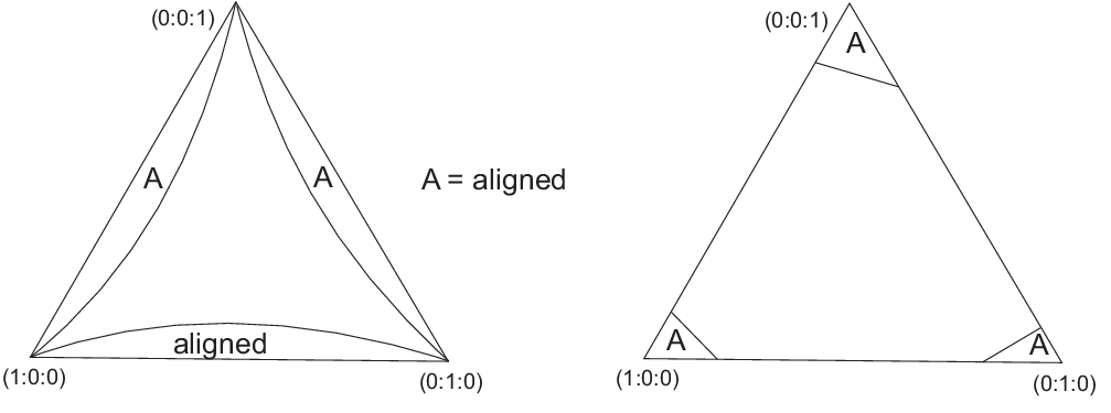
Now let us analyze the meaning of the above theorem from the bifurcation theory viewpoint. By homogeneity we may assume that $q_{1}+q_{2}+q_{3}=1$. Since we only consider positive charges the control space of our system is a triangle $\Delta$. In this triangle the bifurcation set is given by the equalities:

The middle part of $\Delta$ (see Fig. 2, left) corresponds to the case (1) of the above theorem: the minimum is achieved at two mutually symmetric non-degenerate triangles. For the other points of the triangle $\Delta$ all critical configurations are aligned.

The situation we encounter here is a typical example of a (supercritical) pitchfork bifurcation. In the single variable case this is locally described by the potential $f(x,y,\lambda)=\frac{x^{4}}{4}-\lambda\frac{x^{2}}{2}+y^{2}$. Its critical set is given by $x^{3}-\lambda x=0,\;y=0.$ So it consists of a parabola and a line is the $(x,\lambda)$-plane (see Fig. 3). The points on the $\lambda$-axis are critical with value $0$ for all $\lambda$: a minumum for $\lambda<0$ and a saddle point for $\lambda>0$. The points on the parabola are minima with value $-\frac{1}{2}\lambda^{2}$. This is the typical situation for a point on the bifurcation set [3].

We can conclude the following. Assume that we have the charge $q_{2}=0$ whereas the other two charges are non-zero. Then the configuration $(p_{1},p_{2},p_{3})$ considered as a physical system becomes aligned with $p_{1}$ and $p_{3}$ at the endpoints, and the position of $p_{2}$ does not matter. We begin to gradually increase the value of $q_{2}$. As soon as it is non-zero, $p_{2}$ takes some specific position on the aligned configuration (see Lemma 1) (which does not depend on the value of $q_{2}$ while it is small), stays at the same place (we call this fixing effect) until we cross over the bifurcation set, where it moves away from the line. We get two triangles as minima and the aligned position persists as a saddle point in the same position.

Remark. In view of the above, the inverse problem is now solved straightforwardly. Namely,

1. (1)

   If three points in the plane are not collinear, their stabilizing charges are defined uniquely up to a scale.

2. (2)

   If the three points are aligned, the stabilizing charges are defined not uniquely: the charges at the endpoints come from Lemma 1, whereas the charge of the intermediate point has to be small enough.

The direct computation for $n$-gons (even with $n=4$) leads to complicated equations that do not give a transparent solution. However some important qualitative observations can be done. An informal message of the below theorem is that for aligned configurations, there exists fixing effect of the Euler’s Buckling Beam type.

Proof. (1) Assume the contrary. In this case there exists an infinitesimal motion (that is, an element of the tangent space $T_{P}M(n)$) which increases some of diagonals with non-zero derivative, whereas derivatives of all the rest of of pairwise distances is zero, see Fig. 4.

(2) Let us take an aligned configuration which is a critical point. We can assume that it lies on the $x$-axis. Assume that its endpoints are $p_{1}$ and $p_{n}$. In its neighborhood in the space $M(n)$ we choose $(n-2)$ coordinates that correspond to $x$-coordinates of $p_{2},...,p_{n-1}$. The other $(n-2)$ coordinates correspond to $y$-coordinates of the same points. Symmetry arguments $E(\overrightarrow{x},\overrightarrow{y})=E(\overrightarrow{x},-\overrightarrow{y})$ imply that the Hessian matrix is a block matrix

where $H_{1}$ is the Hessian with respect to the $x$-coordinates, that is, the Hessian associated with the one-dimensional ambient space. We are going to show that the Hessian matrix $H_{2}$ related to the coordinates $y_{i}$ is positively definite provided that $q_{2},q_{3},....,q_{n-1}$ are relatively small. Let us assume that $n=4$; the same approach works for $n>4$.

We mimic the proof of formula $(*)$. Namely, we use the symmetry property of $E$ and choose two shifts $y_{1}$ and $y_{2}$. We can choose the coordinates in any symmetric way with respect to $(y_{1},y_{2})$, so let us take $s=t$. Using notations of Fig. 5, from the fixed perimeter condition we conclude that

Therefore

Here $R$ is a sum of fractions with smaller numerator and a denominator that quadratically depend on $y_{i}$. The first summand has an obviously positively definite Hessian and majorates the rest of the summands $R$.∎

We consider three concentric circles with radii $r_{1},r_{2},r_{3}$ and three charges $q_{1},q_{2},q_{3}$ . The correspodning configuration space $T(r_{1},r_{2},r_{3})$ can be identified with a $2$-torus. Let us fix some notation (see Fig. 6):

Note that $d_{i}$ depends on $\alpha_{i}$ via the cosine rule, e.g. $d_{3}^{2}=r_{1}^{2}+r_{2}^{2}-2r_{1}r_{2}\cos\alpha_{3}$.

We suppose that all charges are positive (but similar analysis works also if some of the charges are negative) and that all $r_{i}$ are different. The Coulomb energy

is thus a bounded function on the $2$-torus for each $q_{1},q_{2},q_{3}$.

Proof. This follows by applying Lagrange multiplier method to $E$ with the constraint $\alpha_{1}+\alpha_{2}+\alpha_{3}=2\pi$.∎

An immediate corollary is that the aligned positions (where $\alpha_{i}\equiv 0$ modulo $\pi$) are among the critical points. There are four aligned configurations (see Fig. 7); let us study them first.

Using a parametrization via $\alpha_{1}$and $\alpha_{2}$ we can compute the first and second derivatives of $E$, and evaluate them at the corresponding critical point. The matrix of second derivatives is (in the aligned case):

The Hessian determinant (up to a positive multiple) becomes:

Assume that $\alpha_{1}=\alpha_{2}=\pi\;,\;\alpha_{3}=0$. In this case we have

Therefore we have a linear form

It follows that, for $q_{3}$ big and $q_{1},q_{2}$ small, the Hessian is positive and gets negative on the other side of the line $H=0$ in the affine triangle $\Delta$. The first case corresponds to a local minimum; the second to a saddle point. Again we meet an example of the pitchfork bifurcation: fix $q_{1},q_{2}$ small and let $q_{3}$ start big and decrease next. The system stays at equilibrium minimum in the aligned position until it meets $H=0$; after that the aligned position become a saddle and two minima are born as symmetric triangles.

We give now the final result for all aligned situations.

Also here the control space (with normalized charges) is a triangle. The zero sets of the linear functions from Theorem 4 cut out three small triangles around vertices of this triangle (see Fig. 2, right). They don’t intersect. Each of the triangles corresponds to a minimum state.

Unlike the constrained problem discussed in Section 3, the number of the non-aligned critical configurations is difficult to analyze. They are solutions of the equation in Proposition 2, which seems difficult to solve by hand. We proceed with discussing a few qualitative aspects and mention the results of some tests with Mathematica.

First, the non-degeneracy of $E$ and Betti numbers of the torus imply that there are at least four critical points with sum of their Morse indices is equal to zero. In case of one minimum, two saddles and one maximum we have an exact Morse function. From Theorem 4 we have already four critical points, which includes a single maximum. If the three other points all are saddle points (where this happens can be computed from the above Hessians) then there must be at least two minima which correspond to (non-aligned) triangles. They come in couples via symmetry with the same critical value. Computer experiments suggest that there are no more critical points.

If one of the aligned critical points is a minimum, then two saddles and one maximum could suffice. This is supported by computer tests. Direct computations show that no more aligned minima appear. The existence of the pitchfork bifurcation also implies the existence of (at least) 2 minima for certain values of the $q_{i}$’s.

Observe that the Hessian also depends on $r_{1},r_{2},r_{3}$. Changing these values will also influence the position of critical configurations, including the effect of pitchfork bifurcation. An interesting point is also to take the limit to the equal radius case. In this case we have the following proposition.

As a consequence we have that, for almost equal radii and almost equal charges, the global minimum is achieved at two mutually symmetric triangles that are close to the equilateral one.

The considerations and results of the present paper suggest a few immediate remarks.

(1) The same qualitative behaviour holds for several other central forces, that is, e.g. for the potentials

(2) A natural generalization of the setting suggested in this paper arises if one considers equilibria of point charges lying on several different contours in the plane. In this case Coulomb energy defines a differentiable function on a torus so there are topological restrictions on the number of critical points. It would be interesting to find examples of charges for which the number of equilibria is minimal or maximal.

(3) There apparently exist many other developments for which the results of this paper may serve as paradigms.

References

- [1] P. Exner, An isoperimetric problem for point interactions, J. Phys. A: Math. Gen. A38, 2005, 4795-4802.
- [2] G.Giorgadze, G.Khimshiashvili, On non-degeneracy of certain constrained extrema, (Russian) Doklady Math. 465, No.3, 2015, 1-5.
- [3] M. Golubitsky, D. Schaeffer, Singularities and Groups in Bifurcation Theory, Vol. 1, Appl. Math. Science, 51, Springer, 1985.
- [4] G. Khimshiashvili, Equilibria of constrained point charges, Bull. Georgian Natl. Acad. Sci. 7, No.2, 2013, 15-20.
- [5] G.Khimshiashvili, G.Panina, D.Siersma, Coulomb control of polygonal linkages, J. Dyn. Contr. Syst. 14, No.4, 2014, 491-501.
- [6] G. Khimshiashvili, G. Panina, D. Siersma, Equilibria of point charges on convex curves, J. Geom. Phys. 98, 2015, 110-117.
- [7] G.Khimshiashvili, G.Panina, D.Siersma, V. Zolotov, Point charges and polygonal linkages, J. Dyn. Contr. Syst., to appear. Available online http://link.springer.com/article/10.1007/s10883-015-9286-3/fulltext.html
- [8] T. Poston, I. Stuart, Catastrophe theory and its applications, Pitman, 1978.