$\mu$MECH Micromechanics Library Note: The post-print manuscript of the article published in Advances in Engineering Software, DOI: 10.1016/j.advengsoft.2016.07.010.

Let assume an infinite isotropic homogeneous body with separated heterogeneities, Fig. 1. Moreover, consider the body be the subject to some macroscopic excitation, e.g. a remote strain induced by a combination of displacement and traction fields $\mathbf{u}(\mathbf{x}),\mathbf{t}(\mathbf{x})$ applied to the boundary $\partial\Omega_{0}$ at infinity.

The stiffness of such a composite can be decomposed as [5, 6]

where $\mbox{\boldmath$\mathbf{C}$}_{0}$ represents the fourth order tensor of elastic constants of the matrix $\Omega_{0}$ and $\overline{\mbox{\boldmath$\mathbf{C}$}}(\mathbf{x})=\mbox{\boldmath$\mathbf{C}$}(\mathbf{x})-\mbox{\boldmath$\mathbf{C}$}_{0}$ is its piecewise constant complement to $\mbox{\boldmath$\mathbf{C}$}(\mathbf{x})$ due to the presence of $1,\dots,n$ heterogeneities. Note, $\overline{\mbox{\boldmath$\mathbf{C}$}}(\mathbf{x})$ is nonzero only for $\mathbf{x}\in\bigcup_{r=1}^{n}\Omega_{r}$. As a result of applied loads, the heterogeneous body experiences local fields that can be decomposed by analogy to Eq. (1) as

Here, the superscript $\bullet^{0}$ indicates the homogeneous (macroscopic) component of the state variables in the absence of heterogeneities and $\overline{\bullet}$ stands for its perturbation (microscopic) counterpart induced by their presence. Determination of the perturbation fields is based on the equivalent inclusion method as proposed by Eshelby in [1]. Here, we first limit the exposition to a single ellipsoidal heterogeneity embedded in a homogeneous matrix undergoing a uniform remote strain excitation and then explore some possibilities to take into account interactions among multiple heterogeneities.

When seeking for local fields by means of the equivalent inclusion method, we replace the heterogeneity problem, Fig. 2a, by an equivalent inclusion problem consisting of the homogeneous matrix exposed to a suitable stress-free eigenstrain $\mbox{\boldmath$\varepsilon$}^{\tau}(\mathbf{x})$ which vanishes everywhere except for $\mathbf{x}\in\Omega_{1}$, Fig. 2c, supplement to external loads applied at infinity, Fig. 2b, see [1] for further details.

The solution of the inclusion problem then primarily requires the determination of the transformation eigenstrain $\mbox{\boldmath$\varepsilon$}^{\tau}(\mathbf{x})$ that induces identical perturbation to the homogeneous fields as it would occur due to the original inhomogeneity. As there are no other inclusions surrounding that of our concern, $\mbox{\boldmath$\varepsilon$}^{\tau}(\mathbf{x})$ remains constant in $\Omega_{1}$, that is we can write $\mbox{\boldmath$\varepsilon$}^{\tau}(\mathbf{x}\in\Omega_{1})=\mbox{\boldmath$\varepsilon$}^{\tau}$. According to Hook’s law and decompositions in Eq. (2)^2,3, local stresses rendered by the inhomogeneity problem, Fig. 2a, read as

For the equivalent problem holds

Given the fact that $\mbox{\boldmath$\sigma$}^{0}=\mbox{\boldmath$\mathbf{C}$}_{0}\,\colon\mbox{\boldmath$\varepsilon$}^{0}$, it yields from Eq. (2)³ and Eq. (4)

Now, equating the rhs’s of Eqs. (3–4),

and taking into account the following fundamental solution for $\overline{\mbox{\boldmath$\varepsilon$}}(\mathbf{x})$

where $\mbox{\boldmath$\mathbf{S}$}(\mathbf{x})$ denotes the Eshelby tensor evaluated at an arbitrary point $\mathbf{x}$, results

The definition of $\mbox{\boldmath$\mathbf{S}$}(\mathbf{x})$ tensor is as in Eq. (14) and Eq. (16)¹ while the detailed derivation can be found e.g. in [1, 5]. Finally, Eq. (8) gives rise the sought stress free transformation eigenstrain $\mbox{\boldmath$\varepsilon$}^{\tau}$ in the form

where tensor $\mathbf{Q}$ reads as

Once the transformation eigenstrain has been determined, Eq. (9), the stress perturbation can be computed from Eq. (5) and displacement perturbations as

where the operator $\mbox{\boldmath$\mathcal{L}$}(\mathbf{x})$ is the third order Eshelby tensor-like operator mapping $\mbox{\boldmath$\varepsilon$}^{\tau}\mapsto\overline{\mathbf{u}}(\mathbf{x})$ whose detailed derivation can be found in [2].

The solution to a single inclusion in the infinite matrix loaded by a constant eigenstrain stated formally in equation Eq. (7) was generalized by Sendeckyj (1967) and Moschovidis (1975) for eigenstrains prescribed in a general polynomial form [5, and references therein]. For a simpler exposition, here we summarize only the solution to the single inclusion under linear eigenstrain excitation, though the solution to the problem with quadratic eigenstrains is also implemented to some extent in current version of $\mu$MECH. Going back to index based Einstein summation convention, the prescribed linear eigenstrain field that is nonzero only for $\mathbf{x}\in\Omega_{1}$, is defined as

where $\varepsilon^{\tau}_{ij}$ is the constant part of the imposed eigenstrain identical to that from the previous paragraph, and $\varepsilon^{\tau}_{ijk}$ contains its gradient complements in $k$-th coordinate direction. By analogy to Eq. (7), it holds

The solution thus reduces to seeking for components of tensors $S_{ijkl}$ and $S_{ijklm}$, which depend only on the proportions of the semi-axes of $\Omega_{1}$ and matrix Poisson’s ratio $\nu_{0}$. In particular, for exterior points, i.e. $\mathbf{x}\notin\Omega_{1}$, the following definitions hold [5]

On the other hand, for all points $\mathbf{x}$ inside $\Omega_{1}$, the above tensors read as

Symbol $\delta_{ij}$ denotes the Kronecker delta and $\bullet_{,i}$ stands for the first derivative in $i$-th direction. The potentials $\phi$ and $\phi_{i}$ and the first derivative of potential $\psi$ and $\psi_{i}$ are defined as

with $a_{i}$ being ellipsoidal semi-axe lengths sorted in descending order and index $k$ being the summation index. Elliptic integrals $V$, $V_{i}$ and $V_{ij}$, respectively, read

where $I$, $I_{i}$, $I_{ij}$ and $I_{ijk}$ are $\lambda$-variable dependent elliptic integrals. The value of $\lambda$ for a given point $\mathbf{x}\in\Omega_{1}$ is the largest positive root of the cubic equation

and zero otherwise. The elliptic integrals $I$ and $I_{i}$ are expressed as

with $b=4\pi a_{1}a_{2}a_{3}$, $\theta=\arcsin\sqrt{1-a_{3}^{2}/a_{1}^{2}}$, and $c=\sqrt{(a_{1}^{2}-a_{2}^{2})/(a_{1}^{2}-a_{3}^{2})}$. Functions $F$ and $E$ are the incomplete Legendre elliptic integrals defined as

In addition, higher order integrals $I_{ij}$ and $I_{ijk}$ are expressed by means of those of the lower orders and by substituting $\alpha=(a_{i}^{2}-a_{j}^{2})$ as follows

Finally, $\Delta(\lambda)$ reads as

In the case of an infinite matrix with multiple inclusions, the perturbation fields within $\Omega_{r}$, Fig. 1, are no longer uniformly distributed as a result of their mutual interactions. In $\mu$MECH, we account for the interactions only approximately by assuming the eigenfields within $r$-th inclusion be still constant, however, influenced by local changes of state variables due to the remaining inclusions, namely those nearby $\Omega_{r}$. In particular, we control the “compatibility” of the perturbation strain field inside each inclusion calculated by means of Eq. (7). The key ingredient of these formulas, $\mbox{\boldmath$\varepsilon$}^{0}_{r}$, mapped to $\mbox{\boldmath$\varepsilon$}^{\tau}_{r}$ through $\mbox{\boldmath$\mathbf{Q}$}_{r}$, is recursively increased by perturbation strains $\overline{\mbox{\boldmath$\varepsilon$}}_{s\to r}$ arising from the presence of $s=1,\dots,n$ inclusions. That is why, we have different $\mbox{\boldmath$\varepsilon$}^{0}_{r}$ for each of $1,\dots,r,\dots,n$ inclusions. Individual contributions $\overline{\mbox{\boldmath$\varepsilon$}}_{s\to r}$ to $\mbox{\boldmath$\varepsilon$}^{0,\mathrm{tot}}_{r}$ are measured in the center of $\Omega_{r}$, Fig. 3a. Thus, $\mbox{\boldmath$\varepsilon$}^{0,\mathrm{tot}}_{r}$ in the $p$-th iteration loop of the self-compatibility procedure reads as

where the contributions ${\vphantom{\overline{\mbox{\boldmath$\varepsilon$}}}}{}^{p}\overline{\mbox{\boldmath$\varepsilon$}}_{s\to r}$ are evaluated from the previous remote field ${\vphantom{\mbox{\boldmath$\varepsilon$}}}{}^{p-1}\mbox{\boldmath$\varepsilon$}^{0,\mathrm{tot}}_{r}$; the ${s\backslash r}$ operation excludes inclusion $r$ from the set of $n$ inclusions. The initial remote strain $\mbox{\boldmath$\varepsilon$}^{0}$ is imposed to the matrix surrounding all inclusions at the beginning of the procedure, i.e. ${\vphantom{\mbox{\boldmath$\varepsilon$}}}{}^{1}\mbox{\boldmath$\varepsilon$}^{0,\mathrm{tot}}_{r}=\mbox{\boldmath$\varepsilon$}^{0}$. The line-by-line definition of the iterative algorithm based on Eq. (24) follows in Tab. 1.

At its convergence, the stress and displacement perturbations corresponding to compatible transformation eigenstrains are recalculated according to Eq. (5) and Eq. (11). It is worthwhile to note that the algorithm does not depend on a particular sequence of inclusions, as follows from the elastic reciprocity theorem [7, and references therein]. The iterative procedure has been chosen since a closed form solution for the multiple inclusion problem does not exist and a numerical one would be prohibitively expensive, see e.g. [7]. The computational complexity of the so called full version of the algorithm is $O(n^{2})$. However, this can be further reduced by taking into account only inclusions that have a non-negligible impact on the $r$-th inclusion of interest, usually those placed very nearby $\Omega_{r}$ or excessively large inclusions in the case of somehow disparate polydisperse. This algorithm is called optimized in $\mu$MECH. Its complexity reduces to $O(\xi n)$, where $\xi=\frac{1}{r}\sum_{r}\xi_{r}$ is the arithmetic average of the number of inclusions whose cut outs limited by radii¹¹ 1 A usual choice is $2.5$ multiple of the longest semi-axis $a_{1}$. $\rho_{s}$ centered in $\mathbf{x}_{s}$ embrace the $r$-th inclusion, Fig. 3b. Note, for $n\to\infty$ the complexity of optimized algorithm is $O(n)$ as $\xi=\mathrm{const}\ll n$.

When dealing with a dilute distribution of inclusions, constant strain and stress fields are assumed within $\Omega_{r}$ and no question on concentrations comes in play. However, the goal of $\mu$MECH is to proceed a few steps beyond, namely to non-dilute dispersions. The concentrations arising from mutual inclusion interactions are approximated by the following procedure, which stems from the approximate solution to the sought non-constant transformation eigenstrain $\mbox{\boldmath$\varepsilon$}_{r}^{\tau}(\mathbf{x})$ suitable for the decomposition in Eq. (12) or similar one of a higher degree.

Consider point a $\mathbf{x}$ inside the inclusion domain $\Omega_{r}$, where we calculate the stress free transformation eigenstrain as

Consequently we sample $\mbox{\boldmath$\varepsilon$}_{r}^{\tau}(\mathbf{x})$ in as many points $\mathbf{x}$ as necessary for a polynomial of chosen degree, three in the case case of Eq. (12). Finally, the solution to perturbation fields for points $\mathbf{x}$ in each domain $\Omega_{r}$ are obtained following the exposition given in Paragraph 2.3. For the points within the matrix, i.e. $\mathbf{x}$ outside the union $\bigcup_{r=1}^{n}\Omega_{r}$, the solutions are obtained by the sum of individual contributions attributed to each of $1,\dots,n$ inclusions.

An alternative, and surprisingly well working, approach such that it does not call for the implementation of polynomial eigenstrain problem is, that the solutions to perturbation strains in the internal points are calculated by means of the basic Eshelby formula given in Eq. (7), as

where $\mbox{\boldmath$\varepsilon$}_{r}^{\tau}(\mathbf{x})$ is that provided by Eq. (25). By analogy to the latter approach, the solution in external points is obtained by adding up contributions from all inclusions.

Finally, it is worthwhile to note that the computational complexity can be controlled by the number of internal points chosen to approximate $\mbox{\boldmath$\varepsilon$}_{r}^{\tau}(\mathbf{x})$ by either of the approaches above. In addition, substantial savings can be made by choosing optimized mode running on the same principles as in the case of the self-compatibility algorithm.

Assuming non-elastic phenomena be entirely attributed to the microstructure evolution dynamics, the constitutive behavior of an arbitrary point $\mathbf{x}$ at an instant is governed by the following pair of equations [8],

where $r=0,\dots,n$. According to Hill’s lemma [9, 8], the averages of the above local quantities $\mbox{\boldmath$\sigma$}(\mathbf{x})$ and $\mbox{\boldmath$\varepsilon$}(\mathbf{x})$ are coupled with their macroscopic conjugates $\mbox{\boldmath$\Sigma$},\mbox{\boldmath$E$}$ as

It is evident, that the effective elastic stiffness and compliance tensors depend on the elastic properties of each phase $\mbox{\boldmath$\mathbf{C}$}_{r}$ and volume fractions $c_{r}$. In addition, they depend on mutual interactions given by the intrinsic geometrical arrangement of the phases and the compatibility or equilibrium requirements, encoded in concentration factors $\mbox{\boldmath$\mathbf{A}$}_{r},\mbox{\boldmath$\mathbf{B}$}_{r}$ for which it holds [10, 1]

Plugging the latter definitions in last two terms of Eq. (28) gives

Now, identifying by $r=0$ a matrix phase in which the remaining heterogeneities are fully embedded, and taking into account the fact that $c_{0}\mbox{\boldmath$\mathbf{A}$}_{0}=\mathbb{I}-\sum_{r=1}^{n}c_{r}\mbox{\boldmath$\mathbf{A}$}_{r}$, $c_{0}\mbox{\boldmath$\mathbf{B}$}_{0}=\mathbb{I}-\sum_{r=1}^{n}c_{r}\mbox{\boldmath$\mathbf{B}$}_{r}$, where $\mathbb{I}$ is the fourth order identity tensor, and considering $c_{0}=1-\sum_{r=1}^{n}c_{r}$, yields

where, according to Eq. (1), it holds

From now on, the central question is how to evaluate the concentration factors $\mbox{\boldmath$\mathbf{A}$}_{r}$ and $\mbox{\boldmath$\mathbf{B}$}_{r}$ for a medium with multiple inclusions.

The general structure of $\mu$MECH is briefly outlined in Fig. 5. Basically, it splits in two major tasks, conversion of inhomogeneity problem to equivalent inclusion problem and evaluation of mechanical fields eventually homogenization. The first step is usually most time-consuming, however it needs to be performed only once and the appropriate data can be stored for subsequent analyzes over the same data, geometry and distribution of inhomogeneities to be exact³³ 3 Note again that the primary purpose of $\mu$MECH is feeding FE packages with subscale data.. The second branch of the algorithm can be called repeatedly to evaluate fields at different locations or to run different homogenization algorithms. However, in the single run cases, the code allows analyzes without saving and reading the auxiliary data.

Description of the inhomogeneity problem is required as the input for the first part of the algorithm. It consists of the geometry definitions (centroids, dimensions and rotation of semi-axes), material characteristics of the inhomogeneities and the matrix (Youngs modulus and Poisson’s ratio), and definitions of imposed eigenstrains⁴⁴ 4 Due to the induced pore pressure or thermal expansion for example. and the remote strain tensors. The latter mentioned remote strains are handled as individual load cases and as such their number is arbitrary. The inhomogeneity inputs are converted into the equivalent problem by making use of Equivalent inclusion method and the self-compatibility procedure presented in Section 2. The stored data, if required, are the equivalent transformation eigenstrains $\mbox{\boldmath$\varepsilon$}^{\tau}_{r}$ and local (say internal) Eshelby tensors $\mbox{\boldmath$\mathbf{\mbox{\boldmath$\mathbf{S}$}}$}_{r}$.

In the second part of the algorithm, mechanical fields at user-defined points, including those outside inclusions, are evaluated. Individual $\mathbf{x}$ coordinates can be entered one by one or in arbitrarily large sets, e.g. nodes or integration points of an FE mesh. Calculated fields may be postprocessed with the in-built post-processor and visualized with tools as Paraview, MayaVi, etc.[17, 18]. Another in-built feature is the homogenization of calculated local fields by DIM introduced in Section 2.6. Optionally, users can disable the self-compatibility algorithm and the evaluation of local fields and use alternative micromechanical approaches discussed also therein.

The library is designed in a way a user or a master program invokes the feedback by using a set of C++ functions. Despite, the I/O data flow between $\mu$MECH and a governing instance can be realized via parameters of the interface functions, the exchange by means of files is also possible as it proved to be more practical especially for large number of inclusions. In both cases, the data have a unified syntax. Symmetric tensors are handled in a non-reduced form and together with non-symmetric tensors, e.g. $\mathbf{S}$, are stored in row-by-row vectors, in the so called Iliffe arrays. In 2D mode the input data can be reduced correspondingly, i.e. coordinates may have only two components, $2$-nd order tensors are of dimensions $2\times 2$, etc. In particular, following data are handled by means of files, the inhomogeneity and equivalent homogeneous problem records, grids of point coordinates⁵⁵ 5 it can be e.g. an FE triangulation in which the mechanical fields are evaluated, and finally the sought fields themselves, see Fig. 5. The ASCII Visualization Tool Kit (VTK) format in both legacy and XML variants has been chosen as the native file syntax [19], as it is human-readable and can be visualized directly in a modeler or free visualization tool-kits [17, 18]. Therefore, the data can be easily controlled at any stage of the software development, debugging, or most importantly, in a routine use.

An example of the legacy VTK file with a composite media description is shown in Tab. 2. It describes the 3D matrix with a spherical and an ellipsoidal inclusions loaded by three remote strains. The dimension of the problem is explicitly determined by the “3D” keyword at the beginning of the second line, which is originally reserved for comments. The number of inclusions and centroid coordinates are given in the data block following the keyword “POINTS”. Dimensions and rotation of semi-axes, and material characteristics of each inclusion are listed in the section introduced by “POINT_DATA”. Finally, the data describing the infinite medium are specified in the section preceded by the “FIELD” keyword. In particular, these are Youngs modulus and Poisson’s ratio of the matrix and the remote strain tensors.

The class Problem is the central element, better say a type, of the object-oriented source code and the vast majority of $\mu$MECH features is accessed through its public members. A representative implementation calling crucial functions of the inhomogeneity problem analysis is listed in Tab. 3.

Line 2 is responsible for importing a complete problem description from the VTK file listed in Tab. 2. The data initialization and verification follows in line 3. Line 4 converts the inhomogeneity problem into the equivalent inclusion problem. The data for multiple use of the problem geometry are stored in line 5, if required. As demonstrated in lines 6-9, imports of both, the inhomogeneity and equivalent homogeneous problems work in the same fashion. Clearly, lines 5-9 or 6-9 can be omitted in the case of a single run.

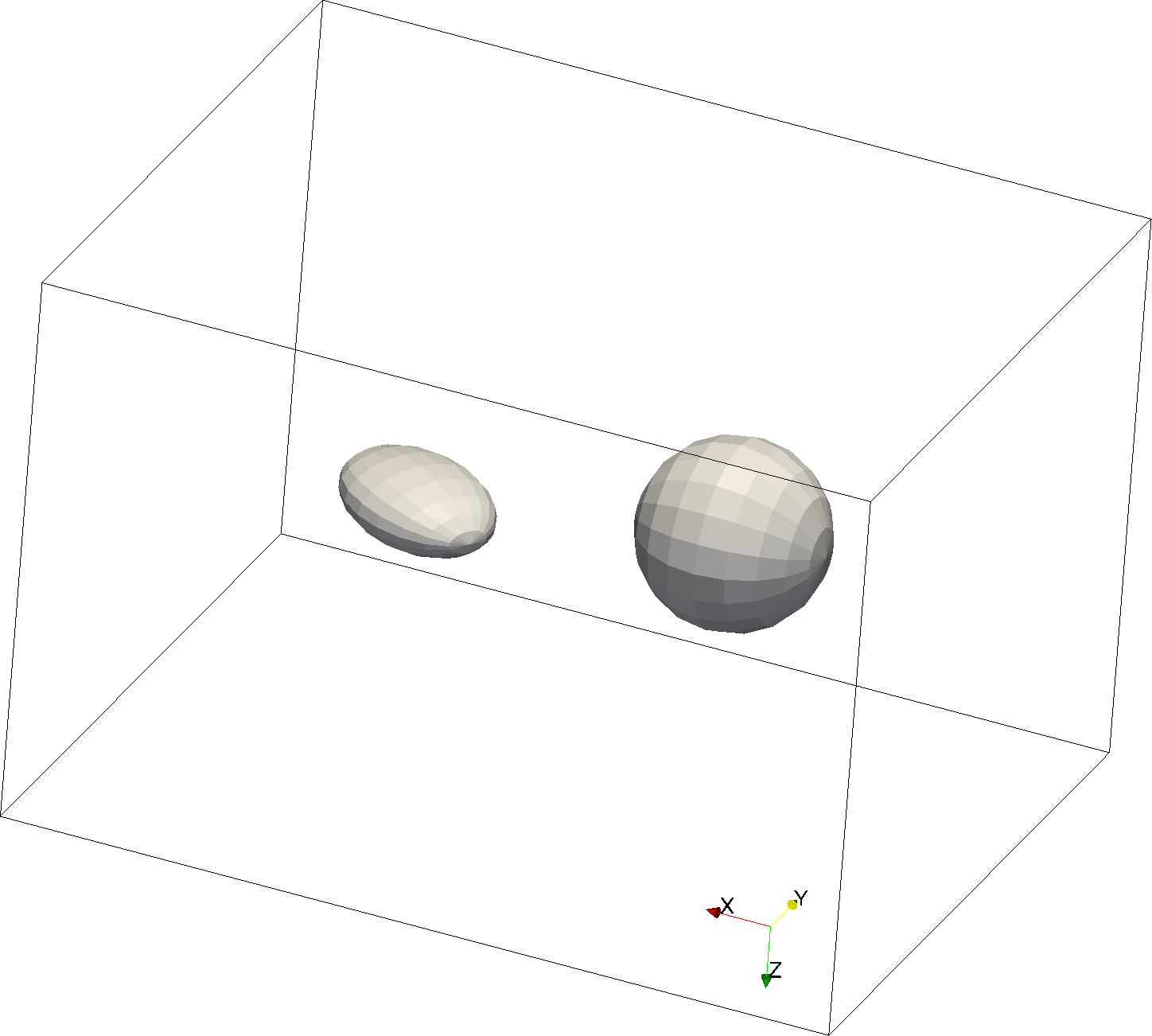
The function giveFieldsOfPoint evaluates mechanical fields at a given point, lines 10-12. Displacement, strain and stress fields are returned by means of the first three parameters, respectively. Each of the parameters is a double pointer to the two-dimensional array. The first dimension is equal to the number of load cases, i.e. remote strains specified at the end of the input file, Tab. 2. The second dimension equals the length of the vector, in the case of displacements, or row-by-row stored tensors when recalling strains or stresses. Passing NULL pointer indicates that the corresponding quantities will not be calculated. The fourth parameter is a pointer to an array of the point coordinates. The next char parameter denotes the character of evaluated fields where ’p’ stands for perturbations while ’t’ for their total counterparts, see Section 2. Finally, the last two parameters determine the index of the first load case and number of load cases to be comprised in the analysis. In this particular case, a pair of perturbation stress tensors due to the first (0-th in C-like syntax) and second remote strain excitations are evaluated in line 12. The data visualized in Paraview are shown in Fig. 6b.

In line 13, function printFieldsOnMeshVTK reads the FE mesh from mesh.vtk file and evaluates total fields in element nodes and the third given remote strain. Then the mesh with results is stored in the file results.vtk. Finally, line 14 performs triangulation of inclusion surfaces which is written in visualization.vtk file. The data visualized in Paraview are shown in Fig. 6a.

A detailed description of other interface functions can be found in tutorial [20] together with a number of ways how to control the analysis, e.g. functions for running different homogenization algorithms, the switch parameter between full and optimal version of either the self-compatibility procedure or evaluation of perturbation/total fields at different points, etc.

$\mu$MECH is a free open source software. It can be run, modified, and redistributed under the terms of the GNU Lesser General Public License as published by the Free Software Foundation; either version 2 of the License, or any later version [21]. The project has been implemented in C++, as it is easier to maintain accessibility of its generic structure while it also enables robust low level optimization of time-consuming algorithms. Multi platform CMake [22] was chosen to configure and build source code properly on client machines. A complete source code and documentation generated by Doxygen [23] script can be found at http://mumech.cz, together with a number of examples and input files by means of which we perform the compilation of an executable file and testing. All interface functions and examples are documented in a tutorial also available at the project website.

References

- [1] J. D. Eshelby, The determination of the elastic field of an ellipsoidal inclusion, and related problems, Proceedings of the Royal Society of London. Series A, Mathematical and Physical Sciences 241 (1226) (1957) 376–396. doi:10.1098/rspa.1957.0133.
- [2] J. Novák, Ł. Kaczmarczyk, P. Grassl, J. Zeman, C. J. Pearce, A micromechanics-enhanced finite element formulation for modelling heterogeneous materials, Computer Methods in Applied Mechanics and Engineering 201 (2012) 53–64. doi:10.1016/j.cma.2011.09.003.
- [3] T. Mori, K. Tanaka, Average stress in matrix and average elastic energy of materials with misfitting inclusions, Acta Metallurgica 21 (5) (1973) 571 – 574. doi:10.1016/0001-6160(73)90064-3.
- [4] M. Šejnoha, J. Zeman, Micromechanics in practice, WIT Press, 2013.
- [5] T. Mura, Micromechanics of Defects in Solids., Martinus Nijhoff Publishers, P. O. Box 163, 3300 AD Dordrecht, The Netherlands, 1987. 587.doi:10.1007/978-94-009-3489-4.
- [6] J. Novák, Calculation of elastic stresses and strains inside a medium with multiple isolated inclusions, in: M. Papadrakakis, B. Topping (Eds.), Proceedings of the Sixth International Conference on Engineering Computational Technology, Stirlingshire, UK, 2008, p. 16 pp, paper 127. doi:10.4203/ccp.89.127.
- [7] B. Pichler, C. Hellmich, et al., Estimation of influence tensors for eigenstressed multiphase elastic media with nonaligned inclusion phases of arbitrary ellipsoidal shape, Journal of Engineering Mechanics 136 (2010) 1043–1053. doi:10.1061/(ASCE)EM.1943-7889.0000138.
- [8] J. Zeman, Analysis of composite materials with random microstructure, Ph.D. thesis, Czech Technical University (2003).
- [9] R. Hill, Elastic properties of reinforced solids: Some theoretical principles, Journal of the Mechanics and Physics of Solids 11 (5) (1963) 357 – 372. doi:10.1016/0022-5096(63)90036-X.
- [10] L. J. Walpole, On the overall elastic moduli of composite materials, Journal of the Mechanics and Physics of Solids 17 (4) (1969) 235–251. doi:10.1016/0022-5096(69)90014-3.
- [11] H. J. Böhm, A short introduction to basic aspects of continuum micromechanics, Cdl-fmd Report 3.
- [12] Y. Guéguen, T. Chelidze, M. Le Ravalec, Microstructures, percolation thresholds, and rock physical properties, Tectonophysics 279 (1-4) (1997) 23–35. doi:10.1016/S0040-1951(97)00132-7.
- [13] R. Hill, A self-consistent mechanics of composite materials, Journal of the Mechanics and Physics of Solids 13 (4) (1965) 213 – 222. doi:10.1016/0022-5096(65)90010-4.
- [14] M. Cai, H. Horii, A constitutive model and fem analysis of jointed rock masses, in: International journal of rock mechanics and mining sciences & geomechanics abstracts, Vol. 30, Elsevier, 1993, pp. 351–359. doi:10.1016/0148-9062(93)91719-Y.
- [15] A. Gavazzi, D. Lagoudas, On the numerical evaluation of Eshelby’s tensor and its application to elastoplastic fibrous composites, Computational Mechanics 7 (1) (1990) 13–19. doi:10.1007/BF00370053.
- [16] J. Vorel, J. Zeman, M. Šejnoha, Homogenization of plain weave composites with imperfect microstructure. part ii. analysis of real-world materials, International Journal for Multiscale Computational Engineering 11 (5). doi:10.1615/IntJMultCompEng.2013004866.
- [17]
Paraview, home page.
URL http://www.paraview.org - [18]
MayaVi, home page.
URL http://mayavi.sourceforge.net - [19]
VTK file format, manual.
URL www.vtk.org/VTK/img/???le-formats.pdf - [20]
muMECH, home page.
URL http://www.mumech.cz - [21]
GNU Lesser General Public
License.
URL http://www.gnu.org/copyleft/lgpl.html - [22]
CMake, cross-platform make, home page.
URL http://www.cmake.org - [23]
Doxygen, home page.
URL http://www.stack.nl/dimitri/doxygen/ - [24] M. Doškář, J. Novák, A jigsaw puzzle framework for homogenization of high porosity foams, Computers & Structures 166 (2016) 33–41. doi:10.1016/j.compstruc.2016.01.003.