Colloidal suspensions of C-particles:
Entanglement, percolation and microrheology
Abstract
We explore structural and dynamical behavior of concentrated colloidal suspensions made up by C-shape particles using Brownian dynamics computer simulations and theory. In particular, we focus on the entanglement process between nearby particles for almost closed C-shapes with a small opening angle. Depending on the opening angle and the particle concentration, there is a percolation transition for the cluster of entangled particles which shows the classical scaling characteristics. In a broad density range below the percolation threshold, we find a stretched exponential function for the dynamical decorrelation of the entanglement process. Finally, we study a set-up typical in microrheology by dragging a single tagged particle with constant speed through the suspension. We measure the cluster connected to and dragged with this tagged particle. In agreement with a phenomenological theory, the size of the dragged cluster depends on the dragging direction and increases markedly with the dragging speed.
pacs
82.70.Dd, 61.20.Lc, 61.20.JaI Introduction
In recent years, the research in the structure and dynamics of colloidal dispersions has shifted from spherical particles to colloids with an anisotropic shape [1, 2, 3, 4, 5]. In particular, various forms of hard non-convex particles can be synthesized by now which are governed by excluded-volume interaction. The non-convex shape gives rise to non-trivial close-packed structures and also affects the dynamics in concentrated suspensions. One of the simplest non-convex shapes is a hard dumbbell, which has been synthesized [6, 7, 8] and was studied quite a lot theoretically [9, 10, 11, 12, 13, 14]. More pronounced non-convexity is realized for colloidal bowls which may penetrate and get stacked [15]. While these are still rotational symmetric shapes, more complex non-convex particles with no rotational symmetry have been considered including bent rods such as banana-shaped [16, 17] and boomerang-shaped [18, 19, 20] particles up to closed rings or tori [21, 22]. Ring-like particles can get completely entangled with important consequence for their dynamics and rheological properties.
In this paper we consider colloidal particles with a horseshoe-like shape which we will refer to as C-particles. These particles are neither rotational symmetric nor convex and play an important role of linking continuously between slightly bent banana-shapes and full tori. The simplest form of a C-shape is a circular part where a segment characterized by an opening angle is cut out from a full circle. If vanishes, a ring-like particle results, while for close to we end up with only slightly bent rods. Therefore, C-particles constitute important interpolating shapes between rods and rings which can show significant, but not perfect entanglement. It is important to note that C-shape colloids can be nowadays fabricated at wish [23, 24] such that our model is realized.
Here, we explore the structural and dynamical behavior of concentrated colloidal suspensions in three spatial dimensions made up by C-shape particles by using Brownian dynamics computer simulations and theory. In particular, we focus on the entanglement process between nearby particles for almost closed C-shapes with a small opening angle . By a suitable definition of entanglement, we associate entangled clusters in the suspension and explore their percolation properties [25]. Connectivity properties have been studied a lot recently by using concepts of percolation theory, in particular in suspensions of rod-like particles with sticky interactions [26, 27, 28, 29, 30, 31, 32, 33], but have never systematically been applied to entangled particles. Depending on the opening angle and the particle concentration, we find a percolation transition for the cluster of entangled particles and identify the percolation threshold. In a broad density range below the percolation threshold, we find a stretched exponential function for the dynamical decorrelation of the entanglement process between a particle pair where is a characteristic time scale for disentanglement. This is similar in spirit, but different in detail due to the fluctuations in shape for ring polymers, to the disentanglement of ring polymers in three dimensions [34, 35, 36, 37], see also Ref. [38].
Finally we study a set-up typical in microrheology by dragging a single tagged particles with constant speed through the suspension. We measure the cluster connected to and dragged with this tagged particle. The size of the dragged cluster depends on the dragging direction and increases markedly with the dragging speed. This is due to a dynamical sweeping-up effects mediated by entanglement. All our predictions can be verified in real-space experiments on colloids by tracking positions and orientations of anisotropic particles [39].
This paper is organized as follows: the model is described in section II. Equilibrium properties are discussed in chapter III including both percolation aspects and the dynamics of disentanglement. Chapter IV is devoted to the non-equilibrium dragging set-up and we conclude in section V.
II Model and methods
II.1 Particle model
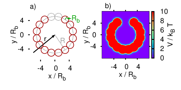
Let us first define our model for C-particles in three dimensions. Ideally we consider a C-particle as composed of spherical hard core beads of radius , as shown in Fig. 1(a). In detail, we start from a full circle (dashed line in Fig. 1(a)) and place in total hard spherical beads along the circle such that they are touching. Then, “missing” beads are removed such that beads remain, which gives rise to the characteristic C-shape and introduces an opening angle
| (1) |
We refer to the plane containing all bead centers as the “symmetry plane” of the particle. The resulting radius of the C-particle (see Fig. 1(a)) is
| (2) |
where the aspect ratio is given by
| (3) |
In three dimensions, a single C-particle has a physical volume of
| (4) |
and its configuration is fully specified by its central position and a set of three angles describing its orientation in space [40, 5].

We now consider a pair of two C-particles, see Fig. 2, which can be characterized by their central positions and and their orientations and . Their interaction is steric or of excluded volume-type, i.e. they are not allowed to overlap. As characteristic for athermal hard-core particles, we assign a vanishing potential energy for a non-overlapping pair and a potential energy of infinity for an overlapping pair, the pair potential is
| (5) |
The following criterion for entanglement of a particle pair is adopted: for a given configuration of two C-particles, their missing spherical beads are formally inserted, i.e. the C-particle is closed to a full ring such that the opening angle would be vanishing. Then there are three possibilities; i) the two rings can be moved continuously away from each other without crossing any energetic barrier, we refer to this as a disentangled pair, ii) the two rings are topologically internested, iii) the two rings physically overlap. By definition, we call configurations entangled if they are not disentangled, i.e. if they belong to either case ii) or iii).
As a first immediate result, we address the excluded volume of two hard C-particles. This quantity measures the degree of steric interactions as embodied in the second virial coefficient and is essential, e.g. in Onsager’s theory of the isotropic-nematic transition [41, 42]. The excluded volume can be defined as
| (6) |
where the orientational average is given by
| (7) |
when is chosen to represent the Euler angles describing the orientation of a rigid particle with non-symmetric shape [40]. By global rotational symmetry, the definition of in Eq. (6) does not depend on . We have calculated the excluded volume for different C-shapes using standard Monte-Carlo simulation [43]. Results for for different particle shapes are presented in Fig. 3 as a function of the contour length
| (8) |
and compared to the straight rod case where [44]
| (9) |

As can be deduced from Fig. 3, the excluded volume of C-particles basically follows that of rods of the same contour length. This is qualitatively different if one excludes entangled configurations, as exemplified for closed rings for which we have calculated without accounting for entangled configurations, see Fig. 3. In fact, for , the scaling of in this case is with , similar to that of thin platelets, also shown for comparison in Fig. 3, where with .
Since hard objects are more difficult to simulate within Brownian dynamics simulations [45, 46, 47, 48, 49], we softened the interaction between two beads and treat them as harsh Yukawa beads. This has been successfully done for rod-like particles under various conditions [50, 51]. We treat the bead-bead pair interactions as
| (10) |
where the parameters were chosen to be and throughout the simulations. The Yukawa-potential is truncated at . The corresponding potential energy landscape felt by a single segment in the neighborhood of a fixed C-particle is shown in Fig. 1(b). The energy quickly increases as the segment approaches the real particle shape such that a mutual crossing in the dynamics is never observed in practice.
II.2 Brownian Dynamics simulation
The motion of colloidal C-particles is governed by completely overdamped Brownian dynamics with thermal noise arising from the solvent. We neglect hydrodynamic interactions between particles, but account for the anisotropic shape of the particles by using an anisotropic mobility tensor. Generally, the diffusion tensor of a particle is given by [52, 53, 54]
| (11) |
where is the grand resistance matrix, which, at low Reynolds number, connects forces and torques acting on particle to its translational and angular velocity. Here, is the thermal energy. The diffusion tensor can be written as
| (12) |
with the pure translational and rotational submatrices and , and coupling translational and rotational motion [52].
Hydrodynamically, the C-particles are approximated as oblate ellipsoids of revolution with major semi-axes of length and a minor semi-axis of length so that the diffusion tensor reduces to
| (13) |
with the analytically known [55, 56, 57] matrices given in Appendix A, which are diagonal in the body frame of the particle. We remark that more sophisticated calculations could be done to match the actual friction coefficients for C-particles better [39, 58], but we do not expect big changes on the disentangle behavior.
This way, rotational and translational motion decouple [52] and the equations of motion are
| (14) |
and
| (15) |
where , is the center of mass of particle , its angular velocity, and the rotation matrix describing the transformation from the body to the laboratory frame. This matrix clearly depends on the orientation of particle , i.e. . Therefore, multiplication with transforms a body frame vector to the laboratory frame, while its inverse does the reverse transformation, e.g. and . Here, primed vectors belong to the body frame, and vectors without a prime symbol to the laboratory frame.
Moreover, the interaction force on particle due to the other particles is given by
| (16) |
where is the force on bead of particle due to the Yukawa-interaction with all other particles’ beads and the sum is over all beads of particle . The corresponding torque is determined by
| (17) |
where denotes the bead center. The stochastic Brownian force is Gaussian-distributed with zero mean and second moment
| (18) |
in the body frame, where the axes are the principal axes of the particle, with and denoting Cartesian components. In close analogy, the Gaussian Brownian torque has zero mean and second moment
| (19) |
in the body frame.

Eqs. 14 and 15 are numerically solved using the standard Euler-forward scheme for stochastic differential equations [59]
| (20) |
and (going into the body frame)
| (21) |
with time step . Here, the Brownian forces and torques have been integrated over time and thus replaced by Brownian translational and rotational moves, and , which are again Gaussian with zero mean and second moment
| (22) |
and
| (23) |
respectively. Moreover, we used Beard and Schlick’s method for bias-free rotational moves [60].
In the simulation, the coupled equations of motion (14) and (15) for C-particles are solved. The time step was made adaptive to limit particle displacement in one single time step to below , with a maximal time step , where the Brownian time is defined as
| (24) |
The orientations of the particles were stored as quaternions, from which the corresponding rotation matrices were computed and which allowed for fast updates of the orientation.
When not noted otherwise, our results stem from simulations of particles with an aspect ratio , see typical system snapshots in Fig. 4. We started with random orientations on equally distributed grid points and then relaxed the system for a time , and gathered statistics until . The cubic system was treated with periodic boundary conditions in all three directions, where the box length is determined by the prescribed volume fraction
| (25) |
of the C-particles. The entanglement criterion as developed earlier was numerically implemented with a piercing technique outlined in Appendix B. For non-vanishing opening angles, , it was carefully checked that the equilibrated system does not exhibit spontaneous nematic ordering but stays orientationally disordered.
III C-particles in equilibrium
III.1 Number of entanglements and percolation

We have calculated the number of entangled pairs per particle, , using the entanglement criterion introduced above. The data in Fig. 5 are shown as a function of since this is the natural representation for infinitely thin C-particles, i.e. if the size ratio , so that the particles radius is the only length scale left. The double-logarithmic plot reveals that the number of entanglements scales as for high densities. For intermediate densities, we find a long crossover which looks to scale as for one to two decades of . The high-density linear scaling can be qualitatively explained with the following argument: Entanglement of one particle can only occur with other particles in a volume around the particle. Since the physical volume is full of particles at high densities, the probability for such particles scales as in this case. Whether the behavior for intermediate density is a real scaling or just a crossover is an interesting question which we leave for future studies.
We assign two particles to be in the same entanglement cluster if there is a chain of entangled particles connecting them. This criterion is symmetric, transitive, and by definition reflexive. Thus, a well-defined sorting of particles is established that divides the system into a discrete set of clusters. As for an example, see the simulation snapshots in Fig. 4 where different clusters are shown in different colors. Near the system percolation transition, the biggest cluster of the system involves a finite fraction of particles in the thermodynamic limit . Data for the biggest cluster are presented in Fig. 6 as a function of the volume fraction (a) and as a function of the reduced density (b). For aspect ratios , i.e. for slender C-particles, there should only be a dependence on the opening angle . Indeed, Fig. 6(b) shows that there is a good scaling on a single Master curve and that both dependencies on and are weak. There is a sharp jump from almost vanishing values for towards a finite value at about for all and which reveals that there is a percolation transition in the system.


Figs. 7 and 8 demonstrate that standard percolation theory [62, 63] applies for this transition. The theory predicts that there is a critical percolation point characterized by universal critical exponents where the biggest cluster fraction is getting non-zero in the thermodynamic limit.
We have checked that two general properties of classical percolation do also apply for our system. First, we have plotted the cluster size distribution function with denoting a size of an entangled cluster in Fig. 7. Below the critical point, the distribution of cluster sizes should follow the law
| (26) |
with the Fisher exponent for undirected percolation in three spatial dimensions [61]. At the critical point, the cut-off size diverges and follows a power law with universal exponent [61], shown as a reference line in Fig. 7. Above the critical point, an exponential decay is seen again, but also a peak at large exists, the so-called giant component. This is indeed confirmed by the data shown in Fig. 7.
Second, we have checked finite system size corrections near the percolation transition. Classical percolation theory [62] predicts that behaves as below the percolation transition, at the percolation transition and above the percolation transitions. The data shown in Fig. 8 indeed confirm these three predictions.
III.2 Long-time diffusion and dynamics of disentanglement
We now address the long-time dynamics as embodied in the mean-square displacement of the center-of-mass coordinate defined as
| (27) |
For short times, the Brownian dynamics is diffusive by construction and the orientationally averaged short-time diffusion constant can be extracted as
| (28) |
For long times , the mean-square displacement is again diffusive, such that we define as usual a long-time self-diffusion coefficient
| (29) |
In general, at finite density, is smaller than its short-time counterpart as the dynamics is hindered by the presence of neighboring C-particles and decreases with increasing density. Numerically, we extract from our simulation data for the mean-square displacement in a finite time window by extrapolating the relaxation in towards long-time diffusion algebraically [64] as
| (30) |
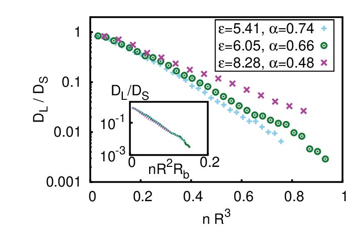
where the amplitude and the time scale are fit parameters to the simulation data. Fig. 9 shows the density dependence of . The inset reveals that a simple exponential dependence on density rescaled with such that
| (31) |
is a good fit for the long-time self-diffusion coefficient over several decades, at least for parameter combinations considered here. This is interesting as convex Brownian hard spheres [65, 66] and hard spherocylinders [46] exhibit an almost linear dependence of on density up to the freezing density. Here, non-convexity and the resulting entanglements slow down the dynamics more drastically, being close to glass formation. In fact, in binary hard sphere mixtures [67, 68] also an exponential increase of the characteristic relaxation time in the density was found for densities not too close to the glass transition. This corresponds to an exponential decrease of as one can extract a typical relaxation time as
| (32) |
which is the characteristic time to diffuse over the size of a C-particle.
We grouped particles with respect to how many entanglements they have on average during the whole simulation length, and then looked at the mean-squared displacements in these groups. For unpercolated systems, we find that the more entanglements a particle has, the more slowly it diffuses. When the system is fully percolated (), there is no more any difference and all particles diffuse with the same constant. This indicates that not only the number of entanglements pins down C-particles and thus hinders diffusion, but that the connectivity is a further obstacle for diffusion.


We now define a dynamical autocorrelation function describing the disentanglement process. First, we define the observable
| (33) |
as an entanglement order parameter and consider its time autocorrelation function, given by
| (34) |
where the brackets denote averages over particle pairs and initial times . Here, the term in the denominator can be further simplified, since . Thereby, is normalized at zero time. Conversely, for long times, the entanglement order parameters are statistically independent such that
| (35) | ||||
As , the long-time limit of vanishes in the thermodynamic limit.

Fig. 10(a) shows data for the entanglement autocorrelation function on a linear scale which exhibit a decay that is significantly slowed down for increasing densities. In fact, a semi-logarithmic plot (see Figs. 10(b,c)) shows that either a normal exponential or a stretched exponential decay in time occurs. The former occurs for small densities as expected, the latter happens for densities which are below but not too close to the percolation threshold. Here, the stretched exponential form
| (36) |
is a good fit to the data which contains the time scale as a typical relaxation time of the disentanglement process. As Fig. 10(c) shows, the value for the exponent is close to 1/2. A similar stretched exponential relaxation scenario is obtained in the context of glass formation where it is better known as a Kohlrausch-Williams-Watt law and results from cage relaxation. Computer simulations [69, 70] as well as experiments and mode-coupling theory [71] give indications that the exponent can be realized in the context of glasses as well.
In fact, the typical relaxation time , defined via , is closely correlated to which sets the time for long-time self-diffusion. This is documented in Fig. 11, where we plot both time scales as a function of the density in the main plot and as a function of in the inset.
At this stage, we remark that the threading of ring-polymers is an analogue to the entanglement of C-particles. These threadings, i.e. one ring penetrating another one, and their influence on the dynamics of a ring-polymer system were explored by simulation in a recent series of papers [34, 35, 36]. Indeed, a significant slow-down of heavily threaded systems and a stretched exponential decay in the time-correlation function of an observable measuring contiguity, i.e. closeness, of two ring-polymers was found where the exponent approaches for sufficiently large rings [36]. Therefore, regarding C-particles and their entanglement as a “topologically driven glass” as introduced in Refs. [34, 35, 36] looks to have merit and might be a fruitful subject for future examinations.
IV Microrheology of C-particle suspensions
We now address a non-equilibrium aspect of C-particles which is closely connected to entanglement. A single “tagged” particle is dragged with prescribed velocity , constituting a set-up of constant-velocity microrheology [72].
IV.1 Simulation scheme
In our constant-velocity microrheology [72] simulations, we suspend the Brownian dynamics move scheme for one “tagged” particle. Instead, its center-of-mass coordinate is moved each time step by , where is a constant unit vector giving the drag direction, is the dragging speed and the particle’s orientation is kept fixed.
First, we consider a situation in which the particle is dragged towards the opening of the C, see Fig. 12(a). As a second case, the probing particle is pulled in exactly the opposite direction. The former favors absorbing new particles into the pulled cluster, while the latter leads to particles slipping off the tagged particle’s cluster. The simulations were started from equilibrated starting positions. The data were then averaged over different runs each lasting 100 .
IV.2 Forward drag
Here, the dragging direction shows from the particle’s center towards the opening of the ring, see Fig. 12(a). During the run, the force on the dragged particle, , was recorded. While it has no effect on the particle’s velocity in our setup, it would have to be compensated in an experimental situation to achieve this constant speed. Therefore it may also serve to define a frictional cluster size as follows. We average the projection of this force onto the drag direction, , and postulate that this is equal to the hydrodynamic drag force of single uncorrelated particles, i.e. we define via the relation
| (37) |
with being the friction coefficient along the -axis of the body frame of a single particle.
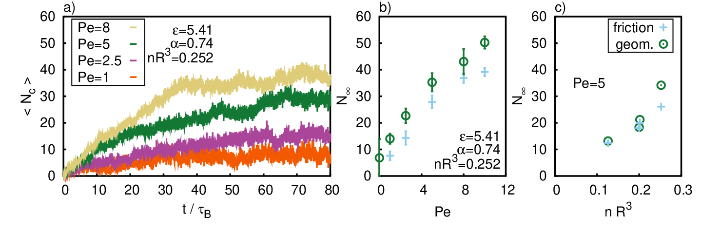
Simultaneously, we measured using the structural entanglement cluster criterion as defined earlier. An example is presented in Fig. 12(b). The structurally-defined cluster size has much higher fluctuations than the frictional one, as is documented also by the corresponding distribution function in the steady state, see Fig. 12(c), which is much sharper for than for . The high overshoots in correspond to situations where blocks of particles are just about to leave the cluster such that they are still counted structurally without having any contribution to the frictional force. Fig. 13(a) shows that the cluster attached to the tagged particle - as averaged over different initial conditions - grows with time, but approaches a finite long-time limit indicative of a steady state.
We shall now model this dynamical process by using phenomenological arguments, following similar ideas as in earlier work [73, 74, 75, 76, 77]. Basically, the cluster dynamics is fixed by two processes, one leading to growth and the other to loss of cluster size. For the growth process we assume that the pulled C-particle collects all particles which it hits with its opening cross section of area . Per time unit it will cover a volume such that on average particles per time unit will be swept up or gathered into the moving C-particle. Each of this particle is connected with other C-particles according to the equilibrium mean size of entangled clusters. Hence, we obtain for the growth process the following rate of particle getting per time unit attached to the moving cluster
| (38) |
Conversely, for the loss process, we assume that a particle only leaves the cluster when its opening shows in the direction of . Assuming single particle rotational Brownian dynamics and an initial perpendicular configuration, the typical time to reach the opening scales with , where is the diffusion constant for rotations around the particle’s normal vector . When a particle strips away, it also removes all entangled particles behind it from the pulled cluster, leading to a proportionality on for the loss rate. As the loss process can result from any individual particle in the cluster, there is an additional proportionality to the actual cluster size such that we get the total loss rate
| (39) |
Combining the two equations, we obtain
| (40) |
where is a numerical constant. With (see Appendix A) and , we arrive at
| (41) |
where is another numerical constant. Solving this ordinary differential equation with the initial condition gives
| (42) |
with the growth time
| (43) |
and the steady-state size of the dragged cluster
| (44) |
where we introduced the Péclet number
| (45) |
Two scaling predictions of our theory are tested in Fig. 13. In Fig. 13(b), simulation data for the steady-state cluster size are shown versus Péclet number Pe for fixed density and there is indeed linear scaling of versus Pe over a broad range of Péclet numbers as predicted by the theory. It is only for high Péclet numbers that deviations from the linear dependence point to the relevance of steric exclusion effects inside the dragged C-particle. Similarly, scales roughly linearly in density for fixed Péclet number Pe, see Fig. 13(c), thereby confirming the theoretical scaling prediction.
IV.3 Backward drag

Let us finally consider dragging a particle away from its opening, where we expect a shrinkage of the dragged cluster. As shown in Fig. 14, the distribution of the pulled cluster size indeed indicates shrinking with increasing Péclet number. In fact, the pulled particle moves mostly alone, no entanglement persists for a longer time. Thus, is getting smaller than its equilibrium counterpart . For extremely large Pe, the mean increases again because the pulled particle encounters more particles which are then part of its cluster for a short time. Hence, interestingly there is a minimum of as a function of Pe.
V Conclusions
In conclusion, we have explored the structure and dynamics of entangling colloidal horseshoe-like particles (referred to as C-particles) by using Brownian dynamics computer simulations. There is a percolation transition of mutually entangled structures which shows a similar signature as percolation in other three-dimensional particulate systems. In the dense regime, the disentanglement dynamics was found to be governed by a stretched exponential demonstrating the dynamical arrest caused by entanglement. Finally, we have found a profound impact of the entangling process on the microrheological behavior where a single particle is dragged through the suspension carrying a whole wake of entangled particles which follow the dragged one. We have identified scaling laws describing this dragged-induced accumulation process.
Our results are in principles verifiable in colloidal suspensions of non-convex particles. Moreover, we expect that most of the qualitative features do also hold for granulates (such as paper-clips etc.) under microgravity [78]. Future work should address the entanglement dynamics in other systems involving particles with other non-convex shapes than considered here. This could maybe include L-particles with a sharp cusp [79, 80] and semiflexible curved polymers (see e.g. Ref. [81]). It would be interesting to check the universality of the disentanglement dynamics. The presence of a sharp cusp in the particle shape is expected to increase entanglement effects significantly.
Acknowledgements.
The authors thank Matthieu Marechal, Liesbeth M.C. Janssen and Peet Cremer for helpful comments. Support from the European Research Council under the European Union’s Seventh Framework Programme, ERC Grant Agreement No. 267499, is acknowledged.Appendix A Diffusion tensor of an ellipsoid of revolution
The following diffusion coefficients for oblate ellipsoids of revolution [55, 56, 57] were used:
| (46) |
and
| (47) |
where is the ratio of the lengths of the long semi-axes and the short semi-axis, and
| (48) |
Here, we used the right-handed coordinate system where is perpendicular to the symmetry plane, is parallel to the line between the particle’s center and the center of its opening, and .
Appendix B Entanglement criterion

In the following, we present a simple criterion of entanglement, for which we just need the distance vector between the centers of mass of two particles and , and the unit vectors and normal to their symmetry planes, see Fig. 15 for an exemplary situation.
The geometrical idea from which we start is the following: Consider the two discs described by the beads of the particles. If there is an entanglement, the first disc’s rim pierces the other disc in exactly one point, and vice versa. If they do not pierce or pierce in two points, there is no entanglement. Thus, the number of piercing points is crucial for entanglement.
All points common to both discs of the particles fulfill
| (49) |
Thus, these points are described by , where and is a vector pointing from the center of mass of particle to the common line. It follows that
| (50) |
We further set
| (51) |
which simplifies Eq. (55), and get
| (52) |
For entangled and , two points are found which lie in both planes, i.e. , and on the line of circle , i.e.
| (53) |
and of which one lies on disk , while the other one does not, i.e.
| (54) |
To check for entanglement, we thus look if such two points exist, i.e. if a pair of with these properties exists.
Combining the ansatz for and Eqs. 51 and 53 leads to
| (55) |
which gives with If there are no points fulfilling the given conditions.
Inserting
| (56) | ||||
into Eq. (54) leads to
| (57) |
These two inequalities are only simultaneously solvable if
| (58) |
For any two given particles, this criterion can be easily checked numerically.
References
- [1] V. N. Manoharan, M. T. Elsesser, and D. J. Pine, Science 301, 483 (2003).
- [2] S. C. Glotzer and M. J. Solomon, Nat. Mater. 6, 557 (2007).
- [3] M. Dijkstra, Adv. Chem. Phys. 156, 35 (2014).
- [4] A. Ivlev, H. Löwen, G. Morfill, and C. P. Royall, Complex Plasmas and Colloidal Dispersions: Particle-Resolved Studies of Classical Liquids and Solids (World Scientific, 2012).
- [5] R. Wittkowski and H. Löwen, Mol. Phys. 109, 2935 (2011).
- [6] P. M. Johnson, C. M. van Kats, and A. van Blaaderen, Langmuir 21, 11510 (2005).
- [7] A. F. Demirörs, P. M. Johnson, C. M. van Kats, A. van Blaaderen, and A. Imhof, Langmuir 26, 14466 (2010).
- [8] S. J. Gerbode, U. Agarwal, D. C. Ong, C. M. Liddell, F. Escobedo, and I. Cohen, Phys. Rev. Lett. 105, 078301 (2010).
- [9] C. Vega, E. P. A. Paras, and P. A. Monson, J. Chem. Phys. 97, 8543 (1992).
- [10] M. Marechal and M. Dijkstra, Phys. Rev. E 77, 061405 (2008).
- [11] K. W. Wojciechowski, D. Frenkel, and A. Brańka, Phys. Rev. Lett. 66, 3168 (1991).
- [12] M. Marechal, H. H. Goetzke, A. Härtel, and H. Löwen, J. Chem. Phys. 135, 234510 (2011).
- [13] F. Chu, N. Heptner, Y. Lu, M. Siebenbürger, P. Lindner, J. Dzubiella, and M. Ballauff, Langmuir 31, 5992 (2015).
- [14] L. P. Fischer, T. Peter, C. Holm, and J. de Graaf, J. Chem. Phys. 143, 084107 (2015).
- [15] M. Marechal, R. J. Kortschot, A. F. Demirörs, A. Imhof, and M. Dijkstra, Nano Lett. 10, 1907 (2010).
- [16] R. Memmer, Liq. Cryst. 29, 483 (2002).
- [17] J. Martínez-González, S. Varga, P. Gurin, and J. Quintana-H, EPL 97, 26004 (2012).
- [18] A. Chakrabarty, A. Konya, F. Wang, J. V. Selinger, K. Sun, and Q.-H. Wei, Phys. Rev. Lett. 111, 160603 (2013).
- [19] A. Kaiser, A. Peshkov, A. Sokolov, B. ten Hagen, H. Löwen, and I. S. Aranson, Phys. Rev. Lett. 112, 158101 (2014).
- [20] A. Kaiser, A. Sokolov, I. Aranson, and H. Löwen, Eur. Phys. J. Special Topics 224, 1275 (2015).
- [21] R. Gabbrielli, Y. Jiao, and S. Torquato, Phys. Rev. E 89, 022133 (2014).
- [22] S. Torquato and Y. Jiao, Phys. Rev. E 86, 011102 (2012).
- [23] S. Sacanna, W. T. M. Irvine, P. M. Chaikin, and D. J. Pine, Nature 464, 575 (2010).
- [24] K. S. Paulsen, D. Di Carlo, and A. J. Chung, Nat. Commun. 6 (2015).
- [25] D. Stauffer and A. Aharony, Introduction to percolation theory (CRC press, 1994).
- [26] H. Meyer, P. Van der Schoot, and T. Schilling, J. Chem. Phys. 143, 044901 (2015).
- [27] M. Mathew, T. Schilling, and M. Oettel, Phys. Rev. E 85, 061407 (2012).
- [28] T. Schilling, S. Jungblut, and M. A. Miller, Phys. Rev. Lett. 98, 108303 (2007).
- [29] B. Nigro, C. Grimaldi, M. A. Miller, P. Ryser, and T. Schilling, Phys. Rev. E 88, 042140 (2013a).
- [30] R. H. J. Otten and P. van der Schoot, Phys. Rev. Lett. 108, 088301 (2012).
- [31] R. H. J. Otten and P. van der Schoot, J. Chem. Phys. 134, 094902 (2011).
- [32] B. Nigro, C. Grimaldi, P. Ryser, A. P. Chatterjee, and P. Van Der Schoot, Phys. Rev. Lett. 110, 015701 (2013b).
- [33] A. V. Kyrylyuk and P. van der Schoot, Proc. Natl. Acad. Sci. 105, 8221 (2008).
- [34] D. Michieletto, D. Marenduzzo, E. Orlandini, G. P. Alexander, and M. S. Turner, ACS Macro Lett. 3, 255 (2014a).
- [35] D. Michieletto, D. Marenduzzo, E. Orlandini, G. P. Alexander, and M. S. Turner, Soft Matter 10, 5936 (2014b).
- [36] D. Michieletto and M. S. Turner, arXiv preprint arXiv:1510.05625 (2015).
- [37] E. Lee, S. Kim, and Y. Jung, Macromol. Rapid Commun. (2015).
- [38] R. Everaers, S. K. Sukumaran, G. S. Grest, C. Svaneborg, A. Sivasubramanian, and K. Kremer, Science 303, 823 (2004).
- [39] D. J. Kraft, R. Wittkowski, B. ten Hagen, K. V. Edmond, D. J. Pine, and H. Löwen, Phys. Rev. E 88, 050301 (2013).
- [40] C. Gray and K. Gubbins, Theory of Molecular Fluids: I: Fundamentals, International Series of Monographs on Chemistry (OUP Oxford, 1984).
- [41] L. Onsager, Ann. N.Y. Acad. Sci. 51, 627 (1949).
- [42] H. N. W. Lekkerkerker and G. J. Vroege, Phil. Trans. R. Soc. A 371, 20120263 (2013).
- [43] D. Frenkel and B. Smit, Understanding molecular simulation: from algorithms to applications, vol. 1 (Academic press, 2001).
- [44] I. Balberg, Philos. Mag. B 56, 991 (1987).
- [45] B. Cichocki and K. Hinsen, Physica A 166, 473 (1990).
- [46] H. Löwen, Phys. Rev. E 50, 1232 (1994).
- [47] A. Scala, T. Voigtmann, and C. De Michele, J. Chem. Phys. 126, 134109 (2007).
- [48] A. Brańka and D. Heyes, Phys. Rev. E 58, 2611 (1998).
- [49] P. Strating, Phys. Rev. E 59, 2175 (1999).
- [50] T. Kirchhoff, H. Löwen, and R. Klein, Phys. Rev. E 53, 5011 (1996).
- [51] H. H. Wensink and H. Löwen, J. Phys. Condens. Matter 24, 464130 (2012).
- [52] J. Happel and H. Brenner, Low Reynolds number hydrodynamics: with special applications to particulate media (Springer Science & Business Media, 1983).
- [53] M. X. Fernandes and J. G. de la Torre, Biophys. J. 83, 3039 (2002).
- [54] M. Makino and M. Doi, J. Phys. Soc. Jpn. 73, 2739 (2004).
- [55] A. Oberbeck, Journal für die reine und angewandte Mathematik 81, 62 (1876).
- [56] D. Edwardes, The Quarterly Journal of Pure and Applied Mathematics 26, 260 (1893).
- [57] F. Perrin, J. Phys. Radium 5, 497 (1934).
- [58] C. Passow, B. ten Hagen, H. Löwen, and J. Wagner, J. Chem. Phys. 143, 044903 (2015).
- [59] D. L. Ermak, J. Chem. Phys. 62, 4189 (1975).
- [60] D. A. Beard and T. Schlick, Biophys. J. 85, 2973 (2003).
- [61] C. D. Lorenz and R. M. Ziff, Phys. Rev. E 57, 230 (1998).
- [62] M. E. J. Newman, SIAM Rev. 45, 167 (2003).
- [63] R. Albert and A.-L. Barabási, Rev. Mod. Phys. 74, 47 (2002).
- [64] H. Löwen, T. Palberg, and R. Simon, Phys. Rev. Lett. 70, 1557 (1993).
- [65] H. Löwen and G. Szamel, J. Phys. Condens. Matter 5, 2295 (1993).
- [66] H. Löwen, Phys. Rev. E 53, R29 (1996).
- [67] A. J. Dunleavy, K. Wiesner, and C. P. Royall, Phys. Rev. E 86, 041505 (2012).
- [68] I. Williams, E. C. Oğuz, P. Bartlett, H. Löwen, and C. P. Royall, J. Chem. Phys. 142, 024505 (2015).
- [69] L. Angelani, G. Parisi, G. Ruocco, and G. Viliani, Phys. Rev. Lett. 81, 4648 (1998).
- [70] E. Rabani, J. D. Gezelter, and B. J. Berne, Phys. Rev. Lett. 82, 3649 (1999).
- [71] W. Götze, Complex Dynamics of Glass-Forming Liquids: A Mode-Coupling Theory, vol. 143 (Oxford University Press, 2008).
- [72] A. M. Puertas and T. Voigtmann, J. Phys. Condens. Matter 26, 243101 (2014).
- [73] G. F. Carnevale, Y. Pomeau, and W. R. Young, Phys. Rev. Lett. 64, 2913 (1990).
- [74] M. Kolb, Phys. Rev. Lett. 53, 1653 (1984).
- [75] E. Trizac and J.-P. Hansen, J. Stat. Phys. 82, 1345 (1996).
- [76] H. H. Wensink and H. Löwen, Phys. Rev. Lett. 97, 038303 (2006).
- [77] P. Cremer and H. Löwen, Phys. Rev. E 89, 022307 (2014).
- [78] K. Harth, U. Kornek, T. Trittel, U. Strachauer, S. Höme, K. Will, and R. Stannarius, Phys. Rev. Lett. 110, 144102 (2013).
- [79] F. Kümmel, B. ten Hagen, R. Wittkowski, I. Buttinoni, R. Eichhorn, G. Volpe, H. Löwen, and C. Bechinger, Phys. Rev. Lett. 110, 198302 (2013).
- [80] B. ten Hagen, F. Kümmel, R. Wittkowski, D. Takagi, H. Löwen, and C. Bechinger, Nat. Commun. 5 (2014).
- [81] T. Iwaki, T. Ishido, K. Hirano, A. A. Lazutin, V. V. Vasilevskaya, T. Kenmotsu, and K. Yoshikawa, J. Chem. Phys. 142, 145101 (2015).