Fast algorithms for Quadrature by Expansion I: Globally valid expansions
Abstract
The use of integral equation methods for the efficient numerical solution of PDE boundary value problems requires two main tools: quadrature rules for the evaluation of layer potential integral operators with singular kernels, and fast algorithms for solving the resulting dense linear systems. Classically, these tools were developed separately. In this work, we present a unified numerical scheme based on coupling Quadrature by Expansion, a recent quadrature method, to a customized Fast Multipole Method (FMM) for the Helmholtz equation in two dimensions. The method allows the evaluation of layer potentials in linear-time complexity, anywhere in space, with a uniform, user-chosen level of accuracy as a black-box computational method.
Providing this capability requires geometric and algorithmic considerations beyond the needs of standard FMMs as well as careful consideration of the accuracy of multipole translations. We illustrate the speed and accuracy of our method with various numerical examples.
Keywords:
Layer potentials; Singular integrals; Quadrature; High-order accuracy; Integral equations; Helmholtz equation; Fast multipole method.1 Introduction
Reformulating the partial differential equations (PDEs) of classical mathematical physics in integral form and then discretizing the resulting integral equation affords several analytic and computational advantages over direct discretizations of the differential operator. For example, integral representations of the solution to exterior boundary value problems inherently capture the correct decay properties at infinity via the use of the Green’s function for the PDE. Furthermore, integral equation formulations are often able to reduce volume discretizations to boundary discretizations, yielding an immediate reduction in computational and storage complexity. Lastly, integral equation formulations frequently reflect the natural conditioning of the underlying physical problem, i.e., well-conditioned physical problems yield well-conditioned integral equations. For concreteness, we consider the method in the setting of the exterior Dirichlet problem for the Helmholtz equation in two dimensions in this contribution. We note however that the method generalizes rather straightforwardly to higher dimensions and different kernels and layer potentials. Consider the boundary value problem [13]:
| (1.1) | ||||
| (1.2) | ||||
| (1.3) |
where is a closed, bounded region with smooth boundary . Equation (1.1) is the Helmholtz equation in , equation (1.2) enforces Dirichlet boundary conditions, and equation (1.3) is the Sommerfeld radiation condition which ensures that the solution is a radiating solution. This boundary-value problem can be reformulated in integral form by representing the solution as a combined-field potential [4, 22]:
| (1.4) | ||||
with the Green’s function
| (1.5) |
where denotes the zeroth-order Hankel function of the first kind [1], and with the unit normal vector at pointing out of . Here, unless otherwise specified, denotes the -norm when applied to a vector, with , and is an unknown density defined on the boundary . This Green’s function also satisfies the Sommerfeld radiation condition
Using this representation of along with the so-called jump relations (cf. (2.1)) and enforcing the Dirichlet boundary condition in (1.2), we obtain the following integral equation along :
| (1.6) |
The operators and , as maps from , are merely and interpreted as principal value and improper integrals, respectively. The operator is known as the single-layer potential, and as the double-layer potential. The efficient solution of (1.6) requires the development of several numerical tools, including quadrature methods for layer potentials with kernels of varying degrees of singularity and, in the setting of iterative methods such as GMRES, asymptotically fast algorithms for computing matrix-vector products with the (notionally dense) matrices resulting from the discretization of (1.6).
Historically, these two numerical tools – quadrature for singular functions and fast algorithms for applying discretized integral operators – have been treated separately. Quadrature methods for singular functions include product integration [15], generalized Gaussian quadrature rules [5, 25], singularity subtraction [16], and many others. See [14] for a recent overview of existing methods. The problem of singular quadrature for layer potentials is, in essence, a local one, in the sense that when the target and source, and , respectively, are well-separated, conventional quadrature rules (such as composite Gaussian) may be applied effectively. As such, the treatment of the singularity may be constrained to the near-field of each piece of the geometry . Such quadrature rules are generally straightforward to couple with fast algorithms such as FMMs because of the natural separation of near-field and far-field calculations.
A somewhat nuanced sub-problem in terms of quadrature appears when the integrand is not singular, but only nearly so. This occurs when targets are located near but not on the boundary . In this sense, targets close to the source geometry present a different challenge than on-surface targets: the corresponding integrals are computable, e.g. by adaptive quadrature, however maintaining efficiency has proven nontrivial for previous methods. Quadrature by Expansion (QBX) [17, 9] originated as an extension of a scheme for nearby evaluation [3], and thus provides a means to handle this difficulty.
In this work, we present a unified algorithm which efficiently embeds Quadrature by Expansion inside a fast multipole method for the two-dimensional Helmholtz equation. The algorithm evaluates both on-surface layer potentials as well as potentials at points arbitrarily near the boundary in a single computation.
QBX was initially described [17] in terms of the underlying analytical idea along with initial theoretical and numerical insight. No fast algorithm was applied, the relevant examples required operations for potential evaluation along a boundary discretized using points. Subsequent work on QBX in [9, 3, 2] is largely foundational, and investigates the rate of asymptotic and convergent approximations of such potential expansions. The goal of this paper, on the other hand, is to make QBX a viable numerical algorithm for the solution to boundary integral equations in two dimensions. The derivation of an algorithm for three dimensions is straightforward using the analogous hierarchical data structures as are described in this work. In order for this to be accomplished, QBX has to be coupled with a fast algorithm such as an FMM. There are several additional considerations that need to be addressed: the effect of adaptive geometry discretizations, orders of multipole and local expansions, and the effective radii of accuracy for translated local expansions. An early version of a fast QBX algorithm was used in [21], but details regarding these topics were not provided.
The paper is organized as follows: In Section 2 we briefly review the details of Quadrature by Expansion for Helmholtz layer potentials and give an informal description of an accelerated algorithm using a standard FMM. In Section 3, we discuss elements of the underlying geometry discretization that will affect the resulting accuracy of the scheme. Sections 4 and 5 discuss additional data structure elements, and how these features adaptively refine the geometry and layer potential densities to ensure numerical accuracy. In Section 6, we discuss the details of using the global QBX scheme to evaluate potentials off (but near) the surface. A detailed description of the QBX scheme embedded into an FMM is given in Sections 7, followed by numerical examples in Section 8. Lastly, in Section 9, the conclusion, we discuss drawbacks of the algorithm of this paper, as well as describe extensions to three dimensions and other PDEs.
2 Background material
In this section we give an overview of the existing QBX scheme, assumptions on the underlying geometry discretizations and the layer potential densities (i.e ), and then provide an informal description of the algorithm. It is important to make a distinction between the on-surface value of the layer potentials and (as an improper or principal-value integral) and their one-sided limits. The one-sided limits of these layer potentials are [18]
| (2.1) | ||||
where we have assumed that the point is located on the curve . Note that the potential is continuous across the boundary , and in both cases, the potentials are smooth up to the boundary with well-defined limits. By and we denote the on-surface restriction of the operators and [18, 7].
Quadrature by Expansion computes the one-sided limits on the right-hand side in (2.1). This is in contrast to classical quadrature schemes for layer potentials which compute the on-surface principal-part of the operator, while one-sided limits are obtained using the jump relations. By computing the average of two different one-sided QBX calculations, as described in [17], one can use QBX to compute the on-surface value of the operator. This approach has certain advantages when coupled with iterative solvers, but this usage is outside of the scope of the current paper.
2.1 Using expansions for quadrature
We next give a precise description of QBX in the case of evaluating in order to establish notation. For a target point near the boundary , the computational task is the numerical evaluation of the integral
| (2.2) | ||||
Using the definition of the Green’s function in (1.5), and the Graf addition formula [20], for not on the boundary , we can rewrite the potential as:
| (2.3) |
The coefficients are known as local expansion coefficients, Fourier-Bessel coefficients, or coefficients of a -expansion. They are given explicitly by:
| (2.4) |
where the polar coordinates of and are with respect to the expansion center , with , located off of and usually along the normal to the curve near . Here denotes the order Hankel function of the first kind and is the order Bessel function of the first kind. This restriction on the location of , relative to and , is necessary to ensure the validity of Graf’s identity. See Figure 1 for a graphical depiction. The -scaled Fourier-Bessel basis satisfies the two-dimensional Helmholtz equation and thus is a natural basis in which to expand potentials.
Even though this expansion was constructed about a point away from the boundary , it can be evaluated at points near, or even on the boundary. In practice, the coefficients in such expansions decay at a rate that depends on the smoothness of and the distance of to the boundary. Truncating this series at index yields an approximation to the potential, with truncation estimates given in [9]:
| (2.5) |
The approximation of integrals for the coefficients via quadrature, and subsequent evaluation of the truncated series (2.5), is the essence of Quadrature by Expansion. This procedure effectively computes the singular or nearly-singular integral by expanding the resulting potential about some point off the surface, and simultaneously, regularizing the integrals corresponding to . Similar expansions to (2.5) exist for various other kernels and layer potentials.
As calculated above, the coefficients will be referred to as global QBX local expansion coefficients since they contain information from all of . We will call an application of QBX with such coefficients Global QBX. This is in contrast to Local QBX, to be described in a future contribution. The algorithm of this paper is concerned with constructing a fast and accurate scheme for the calculation of these global coefficients.
In order to derive the a simple scheme for embedding QBX inside an FMM, it is necessary to place restrictions on the boundary and its discretization. The follow sections outlines our notation for boundary discretization, as well as the restrictions that we place on it.
2.2 Geometry discretization
We assume that the source curve from which we wish to compute the layer potential is discretized by piecewise Gauss-Legendre panels with Gauss-Legendre points on each panel on which the density is represented. We typically discretize panels with , , and points. We sometimes term this the ‘density’ discretization.
We note that in addition to this ‘density’ discretization, we will find it necessary to introduce a ‘source’ discretization consisting of the same panels, each equipped with a larger number of quadrature points, so that the integrals involving density and kernel moments involved in QBX can be computed accurately. Section 3.2 contains the specifics. We will denote the number of source (or quadrature) points on a panel . When needed, point values of the density on the ‘source’ discretization are obtained from the target discretization by polynomial interpolation.
We will use the following notation to refer to nodes and other geometric entities:
- 1.
, the arclength of the panel,
- 2.
, the location of the (‘density’) node on the panel, discretized with respect to arclength,
- 3.
, the outward unit normal to the boundary at the node on the panel,
- 4.
the expansion centers corresponding to node , and
- 5.
, the location of the (‘source’) node on the panel, discretized with respect to arclength,
- 6.
, for denote the location of the targets in the volume at which we wish to evaluate the layer potential.
We note that the targets may reside anywhere in . They are explicitly not restricted to the boundary. Nonetheless, some subtlety is required for targets residing on or near the source curve, see Section 6 for details.
Along the boundary , the continuous density is discretized (sampled) at each of the Gauss-Legendre nodes on each panel in accordance with the Nyström method [19]. For targets sufficiently far away from the boundary , the single-layer potential can then be accurately computed by a -point Gaussian quadrature rule for smooth functions:
| (2.6) | ||||
If the standard -point Gauss-Legendre quadrature weights on the interval are given by , then since it is assumed the nodes are sampled with respect to arclength.
We now turn to the topic of estimating the error inherent in QBX as a numerical methdo, assuming a piecewise Gauss-Legendre discretization of along .
2.3 Estimating the error in QBX
The error in standard quadrature rules (for smooth functions) is usually determined by a single parameter, the order of the quadrature. The error estimates for QBX are slightly more complicated, and consist of two components: the truncation error (related to the decay of the local expansion used) and the quadrature error (i.e. error in computing the coefficients of the local expansion).
As shown in [17], the combined truncation and quadrature error in QBX can be estimated as follows, based on [8, eqn. (2.7.12)]:
Theorem 1
Suppose that is a smooth, bounded curve embedded in , and that , where is the open ball of radius centered at . Let be divided into panels, each of length , and let denote the Gauss-Legendre quadrature approximation to the integral using points. For , there are constants and so that if lies in the Hölder space , then
| (2.7) |
where is the single-layer potential defined in (1.4), and is as in Figure 1.
Remark 1
The quadrature error contains a factor of . Thus, as long as , this factor can be used to control quadrature error by increasing . However, increasing still decreases the quadrature error substantially even if , which the above estimate fails to predict. (We encounter this situation in the determination of in Section 3.2.) More precise error estimates for the QBX quadrature error based on characteristic discretization lengths (i.e. not adaptive discretizations) are discussed in [2].
2.4 Informal description of the algorithm
With the method of QBX and the previous error estimates in mind, an accelerated scheme for the computation of can be derived. This global, accelerated FMM-based QBX algorithm involves three basic steps:
- Step 1
First, we refine the discretization of the boundary and the density to ensure the validity of the error estimate (2.7). For this discretization, we then place one QBX expansion center per ‘density’ node.
- Step 2
Using a modification of the FMM for the two-dimensional Helmholtz equation, we evaluate the potential at all targets, and construct a (QBX) local expansion at the expansion centers that were placed in Step 1 using translations of the FMM-computed Bessel function expansions.
- Step 3
Finally, we identify targets that are close to the boundary (i.e. such targets where the underlying Gaussian quadrature rule fails to accurately approximate the singular or near-singular integral), and re-evaluate the potential using the (QBX) local expansions of the expansion center closest to the target.
The remainder of the paper is dedicated to filling in the details surrounding each of these steps.
3 Accuracy control for global QBX
As noted in Theorem 1, QBX incurs two (additive) error components, truncation error and quadrature error. The truncation error stems from using a truncated -expansion to approximate the (smooth) layer potential, whereas the quadrature error arises from computing the expansion coefficients using numerical quadrature. We now discuss some practical sufficient conditions under which the method yields potentials that are pointwise convergent of order in the maximum panel length up to a user-supplied precision . To achieve this, we ensure that (a) the assumptions of Theorem 1 apply, and (b) the quadrature error does not exceed . Note that we make no attempt to characterize truncation error beyond high-order convergence.
3.1 Controlling truncation error
Truncation error in QBX is tied to the decay of the coefficients of the local (Fourier-Bessel) expansion used to evaluate the potential near the surface. The decay of these coefficients reflects the smoothness of the expanded potential, and the smoothness of the potential in turn is controlled by the proximity of any source geometry. Theorem 1 assures high-order convergence as long as there is no source geometry on the interior of the expansion disk. As such, controlling truncation error in QBX is mainly a geometric matter.
Given our choice of expansion radius for all centers associated with sources on panel (cf. Sec. 2.2), satisfying the assumptions of Theorem 1 amounts to satisfying the following condition. Here and in the following, denotes the Euclidean distance function as applied to points and sets of points.
Condition 1 (Expansion disk undisturbed by sources)
To ensure that no source geometry interferes with the decay of the coefficients of the local expansion, we demand that the distance between the source geometry and each center be at least the radius of that center’s expansion disk, i.e.
| (3.1) |
for all nodes and panels . Breaking down the source geometry further, we may equivalently enforce
| (3.2) |
for all nodes and panels and .
Under Condition 1, the truncated Fourier-Bessel expansion
is a -order approximation to for all targets , up to a precision given by the quadrature error, discussed next.
3.2 Controlling quadrature error
Quadrature error in QBX is estimated in the second term in Theorem 1, i.e. it is mainly controlled by the quantity . In a way, this term measures the amount of resolution supplied to numerically integrate singularities at a distance . Notionally, two mechanisms exist for controlling this resolution–the panel length and the quadrature order . Since we have chosen to proportionally tie the distance of the singularity to the panel length , we do not expect the quadrature error to change in response to mesh refinement, i.e. shrinking the panel length . Thus the remaining instrument to control quadrature error is the number of quadrature points on each panel. Below, we present an empirical procedure to determine a suitable value for for a given kernel to satisfy a user-specified accuracy bound .
Before we do so, we would like to highlight a family of situations that threaten the accuracy of the evaluated layer potentials through an increase in the quadrature error. Consider a source discretization consisting of source panels with unequal panel lengths contributing to the coefficients at a single expansion center belonging to a ‘target’ panel .
If in is chosen so as to only provide sufficient quadrature resolution from panel to its own centers , then no variability in panel lengths can be tolerated without risking insufficient quadrature resolution being available in some source panel/center combinations. Consider a panel with length adjacent to the panel belonging to the current expansion center . While the center-to-source distance in typically does not obey a larger lower bound on than , the increase in the numerator leads to a worse error estimate. Such a situation is common in adaptively refined meshes which we wish to permit. To mitigate the impact of this effect, we enforce the following condition:
Condition 2 (Two-to-one length restriction between adjacent panels)
If panel and panel are adjacent to each other, then
We may then choose so that still satisfies the required accuracy bound, and we therefore tolerate 2-to-1 panel sizing steps in adaptively refined meshes.
Unfortunately, the impact of differing panel sizes is not only felt in adjacent panels. Rather, in the expansions at center , quadrature error originating from, say, source panel , is controlled by . The left half of Figure 5 illustrates a situation in which inaccurate evaluation may occur. If was chosen to satisfy accuracy constraints, then enforcing
ensures that the error contribution of other source panels will not exceed that of . Using our choice , this leads to the following condition, which we will algorithmically enforce.
Condition 3 (Sufficient quadrature resolution from all source panels to all centers)
For each expansion center , the distance from the center to all source panels must at least be commensurate with the source panel’s length , or larger, to ensure adequate quadrature resolution:
We note that the task of enforcing Condition 3 is somewhat challenging owing to its all-pairs (“all sources to all centers”) nature. A fast (non-quadratic) algorithm for its enforcement will be presented in Section 5.2.
In the setting of the Helmholtz equation, the Helmholtz parameter (and the length scale of wave features associated with it) represents a final aspect that may impact the quadrature error. To avoid issues of this nature, we require that source discretization panel lengths are bounded with respect to this length scale, as expressed by the following condition.
Condition 4 (Panel size bounded based on wavelength)
The panel size is bounded with respect to the wavelength.
Returning to the choice of the number of Gauss quadrature points per panel to satisfy a user-specified relative accuracy bound , we note that Theorem 1 provides no explicit way to estimate the constant . While work such as [2] does provide explicit, non-asymptotic formulas for the quadrature error, we note that these are, by necessity, kernel-dependent. In the interest of generality, we describe a numerical procedure, to be carried out once per kernel, that finds a suitable number for each given accuracy target .
We wish to convert the condition
to one that can, at least approximately, be verified once for all panels . To this end, we first rescale so that , so that an expansion center at distance would appear at a distance from the unit-length panel. Next, we reduce to two ‘generic’ panel configurations, a straight panel and a curved panel (cf. Figure 2). For all centers at a distance of of the panel length, we ensure that the coefficient integrals
are computed to within the specified accuracy by adjusting . As can be seen in the figure, for the straight panel, we consider test centers on one side of the geometry (for symmetry reasons), while we consider centers on both sides for the curved one.
This test is accomplished through self-convergence, i.e. by increasing until the changes in the computed integrals in response to resolution increase are below the specified threshold. The tests are carried out with (cf. Condition 4) and with densities , where is the degree Legendre polynomial for . Results of this experiment are summarized in Table 1, for various choices of the accuracy parameter .


| 2 | 8 | 16 | 24 | 32 |
| 4 | 12 | 24 | 32 | 40 |
| 8 | 16 | 32 | 40 | 48 |
| 16 | 32 | 48 | 64 | 64 |
If the four conditions derived in this section are obeyed, then the local expansion coefficients for each QBX expansion centers calculated via the oversampled discretization given by
| (3.3) |
for approximate the exact local expansion coefficients of the single layer potential, defined in equation (2.4), to the prescribed tolerance . In addition, we remark that for locations not covered by QBX expansion disks, unmodified Gaussian quadrature
| (3.4) |
approximates the true potential to the prescribed tolerance . We note that such targets satisfy
As a result, by evaluating QBX expansions where available and using the ‘direct’ Gauss-Legendre computation (3.4) everywhere else, we obtain an -accurate approximation of the layer potential in all of .
3.3 Summary
We have derived four sufficient conditions that, if satisfied, guarantee sufficient accuracy in the evaluation of the layer potential. They are summarized below:
- Condition 1
-
Expansion disk undisturbed by sources.
for all panels numbers and .
- Condition 2
-
Two-to-one length restriction between adjacent panels. If panel and panel are adjacent to each other, then
- Condition 3
-
Sufficient quadrature resolution from all source panels to all centers.
for all panels numbers and .
- Condition 4
-
Panel size bounded based on wavelength.
These conditions reduce the problem of accurate layer potential evaluation to one of ensuring the validity of these four geometric conditions. By inspection of each condition, it is clear that if a given input discretization is found to be in violation of any of the conditions, refining (i.e. splitting all offending panels into two equal-length pieces) until all conditions are obeyed is an effective remedy.
Conditions 2 and 4 are trivially checked by local computation, one panel at a time. The other two conditions however are non-local in character, since they concern pairs of (not necessarily related) sources and centers. While they are trivial to verify by iterating over all such pairs, doing so would negate the benefit of the fast algorithm being derived in this contribution, since it would revert the run time of the algorithm to scaling with the square of the input size, rather than (nearly) linearly.
We finally note that the above family of conditions is technically entirely independent of the FMM (or any other acceleration scheme). It simply represents a family of conditions to ensure that Global QBX (in which the expansions represent contributions from the entire source geometry) to be accurate. It is however natural to consider the computational verification of these conditions in conjunction with an FMM, since the tree data structures already available in this setting can be put to excellent use.
4 Area Queries in Quad-Trees
Conditions 1 and 3 of the previous section were found to involve non-local properties of the input source discretization. We note that being able to efficiently answer queries of the following type is useful in the process of verifying both conditions:
Prototypical query (PQ): Given a collection of points , with an associated radius , identify the collection of targets that are contained in .
The goal of this section is to design an algorithm to complete precisely this task in CPU time.
Quad-tree data structures (such as those constructed by the Fast Multipole Method [12] base of the present algorithm) are well-suited for such tasks. Consider the following setup of an adaptive quad-tree. Let be the smallest square centered at the origin which contains all particles. Particles may be comprised of any combination of sources, targets, expansion centers, and centers of mass of all panels, depending on the procedure. We next introduce a hierarchy of meshes on the computational domain . Mesh level corresponds to and mesh level is obtained by splitting boxes at level into four quadrants, denoted children of the parent box. In order to allow for adaptivity, we allow for different levels of refinement in different regions of . Empty boxes are pruned. Let denote the set of non-empty boxes at level . We will refer to the result of this procedure as a quad-tree on the computational domain .
Remark 2
In a quad-tree, a box is subdivided into equal parts if it contains more than some pre-specified number of particles, . It should be noted that not all categories of particles are considered for determining whether will be subdivided. For example, in a quad tree containing all sources, targets, and expansion centers, can be partitioned if it contains more than sources, regardless of the number of targets, and expansion centers in . This subdivision criterion is decided depending on the procedure, and is user-specified.
To answer queries of type (PQ) given a source in a leaf box , it is not sufficient to check all targets in box and the list of boxes adjacent to as the size of the box and its adjacent boxes is independent of the extent of . It is also unsatisfactory to answer these queries by traversal from the root, since placement of the query box near boundaries of the tree boxes will lead to expensive traversals of much of the tree structure.
Instead, to accommodate these geometry queries, it is sufficient to augment conventional adaptive quad-tree data structures by adding the capability to identify the minimal collection of leaf boxes which completely contain a specified local neighborhood . Our proposed modification to the standard quad-tree consists of an additional iteration structure available on the quad-tree, an operation we term an area query, defined as follows.
Definition 1 (Area Query)
Given:
- 1.
A quad-tree partitioning of a square , and
- 2.
a square with ,
an area query provides
- 1.
a list of all leaf (childless) boxes, , in the quad-tree for which .
Note that while the point needs to lie in , is not required. A simple way to ensure that all relevant points are contained in is to include them as points on which the quad-tree is built.
4.1 Peers
While the area query is conceptually easy to understand, care must be taken that its actual implementation is efficient. To this end, we first define the notion of a peer box.
Definition 2 (Peer Box)
Given a box in a quad-tree, is a peer box of if it is
- 1.
adjacent to ,
- 2.
of at least the same size as (i.e. at the same or a coarser level), and
- 3.
no child of satisfies the above two criteria.
Recall from the original adaptive FMM [6] that a colleague is an adjacent box at the same level. A peer box is similar, however a box at a coarser level may be included in the set of peer boxes if a colleague at the same level fails to exist. Figure 4 shows an example. The box itself is included in its list of peers. Any box (in two dimensions) has at most nine peers.
4.2 Performing Area Queries
To process a single area query for the region , as in Definition 1, we first determine the guiding box associated with the region . Referring to Figure 4, the guiding box for the query, is the smallest box which contains such that is completely contained in the peers of . The algorithm below identifies all leaf boxes resulting from the area query associated with .
Algorithm for area queries
| Comment [Determine guiding box of query] | ||||
| Set to be the root box . | ||||
| do | ||||
| if , | ||||
| break out of the loop, | ||||
| else if has a child containing , | ||||
| find the child of containing , set , | ||||
| else | ||||
| break out of the loop, | ||||
| end if | ||||
| end do | ||||
| Comment [Enumerate and check leaf descendants of peers of ] | ||||
| do | ||||
| do | ||||
| if , | ||||
| include leaf box in the resulting set for the area query. | ||||
| end if | ||||
| end do | ||||
| end do |
In the above algorithm and in the following, by we mean the radius of the box , i.e. the axis-aligned distance from the center of the box to its edge. For example, a unit box has size . Practical implementations can be designed to take advantage of concurrency and locality of data access by processing a large number of area queries in batch form.
The area query mechanism improves on a simple generalization of the quad tree where macro-sources have a specified interaction extent. Area queries ensure that the length-scale of the macro-source is commensurate with the box structure being used for geometric look-up. The three main advantages of area queries are: (a) it is trivially parallelizable, (b) although presented here in two dimensions, it generalizes directly to three-dimensional geometries, and (c) it is competitive in operation count with other algorithmic options that we have explored for detecting regions of validity for QBX expansions.
4.3 Complexity and Correctness
The two following lemmas are straightforward to prove using arguments based on the structure of standard quad-trees.
Lemma 1
The area query algorithm of Section 4.2 performs work, where is the number of levels in the tree, and is the number of leaf boxes being returned by the query.
This complexity estimate is readily apparent from the algorithm above, as there are at most iterations of the loop locating the guiding box , the number of peers of a box is bounded by a constant, and the number of descendants of exceeds the number of boxes returned by at most a constant factor.
Lemma 2
If a box is returned from the query, it necessarily is a leaf box overlapping . Conversely, let be a leaf box overlapping . Thus . Let be the area query’s guiding box. Then . Note that and . Combining these facts yields
Therefore, ’s peers cover at least the area given by , so must be a child of one of the peers of and thus was examined and returned by the area query.
5 Triggering Source Refinement
Using the area query algorithm of the previous section, we next describe algorithms to verify the conditions of Section 3.3. In addition to merely detecting violations, the algorithms further attribute the detected issues to one or more panels which may then be refined. Upon refinement, the conditions are rechecked, and, if necessary, additional rounds of refinement and checking are performed, until all conditions are satisfied.
On refinement, a flagged panel is subdivided into two panels of equal arclength, determined via the Legendre expansion describing the panel’s parametrization. As discussed earlier, Conditions 2 and 4 are easily checked one panel at a time. In this section, we outline algorithms to flag panels based on Conditions 1 and 3.
5.1 An Algorithm to Verify Condition 1
For notational convenience, we refer to expansion centers and sources with a single index. For determining panels which violate Condition 1, if is the center of mass of panel , then let be the smallest radius such that the entire panel is contained in an ‘disk’ of radius centered at , i.e.
| (5.1) |
Next, let denote the list of panels overlapping a leaf box , so that if . It is straightforward to construct this list using an area query on and its associated bounding square .
Let be the expansion center associated with node on panel . Let , and let denote the area query search domain associated with . For each leaf box returned by the area query, we loop over all panels in and flag panels which violate Condition 1. The algorithm below identifies all such panels.
Algorithm for triggering refinement based on Condition 1
| Comment [Choose main parameters] | |
| Create a quad-tree on the computational domain containing all expansion centers and centers of mass of all panels. | |
| Choose the maximum number of particles in a childless box. | |
| Subdivide a box if it contains more than expansion centers. |
Stage 1.
Comment [Refine the computational cell into a hierarchy of meshes for sorting expansion centers, and centers of mass of all panels.]
| do | ||||
| do | ||||
| if contains more than particles then | ||||
| subdivide into four boxes, ignore (prune) the empty boxes formed. | ||||
| end if | ||||
| end do | ||||
| end do | ||||
| Comment [Let be the total number of boxes.] | ||||
| Comment [Let and denote the list of panel centers of mass and expansion centers in box respectively.] |
Stage 2.
| Comment [Loop over all panel centers of mass in every leaf box. Using area queries, identify the list of panels | |||||
| relevant for each leaf box .] | |||||
| do | |||||
| if is childless then | |||||
| do | |||||
| Perform an area query for the region to identify the list of leaf boxes . | |||||
| do | |||||
| Append panel to | |||||
| end do | |||||
| end do | |||||
| end if | |||||
| end do |
Stage 3.
| Comment [Loop over all expansion centers in every leaf box. Using area queries, loop over all relevant | ||||||
| panels to find expansion centers which violate condition 1 and flag the corresponding panel.] | ||||||
| do | ||||||
| if is childless then | ||||||
| do | ||||||
| Perform an area query for the region to identify the list of leaf boxes . | ||||||
| do | ||||||
| do | ||||||
| if where is an expansion center associated with a source on panel , | ||||||
| and , then Flag panel . | ||||||
| end do | ||||||
| end do | ||||||
| end do | ||||||
| end if | ||||||
| end do |
5.2 An Algorithm to Verify Condition 3
To determine panels which violate Condition 3, we carry out the following algorithm. If is (again) the center of mass of panel , then let be the smallest radius such that
| (5.2) |
Note that is a tubular neighborhood around panel , and is a bounding square centered at the panel’s center of mass containing .
If an expansion center on panel lies in defined in equation (5.2), with , and panel is not adjacent to panel , then panel will be flagged. will be the area query search domain associated with to search for centers which may receive insufficiently resolved quadrature contributions from . The algorithm below identifies all such panels. The left-hand side of Figure 5 illustrates the general situation being detected, the right-hand side clarifies the notation.
Algorithm for triggering refinement based on Condition 3
Comment [Choose main parameters]
| Create a quad-tree on the computational domain containing all expansion centers and centers of mass of all panels. |
| Choose the maximum number of particles in a childless box. |
| Subdivide a box if it contains more than expansion centers. |
Stage 1.
Comment [Refine the computational cell into a hierarchy of meshes for sorting expansion centers, and centers of mass of all panels.]
| do | |||
| do | |||
| if contains more than particles then | |||
| subdivide into four boxes, ignore (prune) the empty boxes formed. | |||
| end if | |||
| end do | |||
| end do |
Comment [Let be the total number of boxes.]
Comment [Let and denote the
list of panel centers of mass and expansion centers in box , respectively.]
Stage 2.
Comment [Loop over centers of mass of all panels in every leaf box. Using area queries, loop over all relevant expansion centers to find expansion centers which violate Condtion 3 and flag the corresponding panel.]
| do | |||||
| if is childless then | |||||
| do | |||||
| Perform an area query for the region to identify the list of leaf boxes (cf. Figure 5, right panel) | |||||
| do | |||||
| do | |||||
| if , where is an expansion center associated with a source node on panel , | |||||
| with and panel is not adjacent to panel then flag panel . | |||||
| end do | |||||
| end do | |||||
| end do | |||||
| end if | |||||
| end do |
6 Evaluating Layer Potentials in the Volume
QBX-type expansions of the potential can be used not only to accurately evaluate on-surface, but also near-surface potentials [3]. It is thus expedient to present an algorithm that similarly unifies the treatment of potential evaluation at any target, regardless of whether it is located on, near, or far from the source geometry. This section presents an efficient geometric algorithm based on area queries that enables the subsequent fast algorithm to provide this capability.
6.1 Marking Targets for Evaluation by QBX
The objective of this section is to describe an algorithm to determine, for each target point , whether a ‘conventional’ evaluation of the potential based on Gaussian quadrature and the (point-based) FMM is sufficient, or whether evaluation of the potential through a QBX expansion is required (and if so, which of the many available centers should be chosen). As discussed in Section 3.2, the potential at targets which satisfy needs to be evaluated through a QBX expansion. We will refer to this tubular domain close to the boundary as given by:
| (6.1) | ||||
For efficiency, the algorithm proceeds in three stages:
- 1.
Set up ‘tunnel’ area queries around source geometry to mark region in which potentially inaccurate layer potential evaluation can occur. Figure 6 illustrates the area query being performed.
- 2.
Tag leaf boxes covered by area queries with ‘endangering’ source geometry
- 3.
Based on leaf box containment and tagging information from previous step, decide (a) whether the potential at a center needs to be evaluated through QBX and (b) whether a corresponding center is available.
Associate volume/surface targets with QBX expansions
| Comment [Set up source area query] | |||
| do (panels) | |||
| do (sources on panel ) | |||
| Find bounding squares containing the disks about centers with radii | |||
| Find bounding square centered at so that | |||
| end do | |||
| end do |
| Comment [Mark boxes with nearby sources] | ||
| Perform an area query over the squares | ||
| do in each of the resulting leaf boxes | ||
| Add to the set | ||
| end do |
| Comment [Decide target association] | ||||
| do for each target | ||||
| Find leaf box containing | ||||
| if | ||||
| Mark as requiring evaluation by QBX | ||||
| end if | ||||
| Comment [Locate closest eligible QBX center] | ||||
| if were found then | ||||
| mark to use the QBX expansion around | ||||
| else | ||||
| if was marked as requiring QBX | ||||
| fail target association | ||||
| else | ||||
| mark for evaluation without QBX | ||||
| end if | ||||
| end if | ||||
| end do |
The tolerance in the algorithm is used to ensure that a target point located on the source geometry is properly associated with QBX centers on the source geometry in the presence of inexact arithmetic.
In addition, it should be remarked that the expansion disks do not fully cover the area immediately surrounding the source geometry. Some gaps remain. Algorithmically, we could approach this issue via refinement or by adding additional centers. Empirically, increasing to cover any targets in this region leads to no decrease in accuracy. This is mathematically at least plausible since the expanded layer potentials are very smooth even in the immediate neighborhood of the source geometry, and hence the terms of the QBX expansion grow slowly.
It is straightforward to see that the area query algorithm finds a superset of the targets located in . To determine whether a target is actually located within , one may employ Newton’s method to find the closest point on the panels , or as an approximation, one may use
If accurate evaluation of the layer potential on both sides of the geometry is desired, it is straightforward to augment the presented scheme with a side-preference mechanism that restricts eligible QBX centers to ones on a predetermined side of the geometry. This is particularly important for points located on the source geometry, since for these targets it is impossible to determine which of the two limits is desired by geometric location alone.
7 A Fast Algorithm for QBX
Given a tolerance, , and the number original of Gauss-Legendre points per panel, , we determine from Table 1. As a pre-processing step, we interpolate the discretized geometry and density from the density grid to the source grid As in (2.6), we then approximate the layer potential using the sum
| (7.1) |
For notational convenience, we rewrite the above sum as
| (7.2) |
where . We also approximate the -expansion coefficients at the expansion center using the same source-grid Gauss-Legendre quadrature rule:
| (7.3) |
for , , and . Again for notational convenience, we rewrite the above expression as
| (7.4) |
for . In a minor abuse of notation, we will interchange and when discussing discrete sums. The task at hand is to accelerate the computation of:
- 1.
the potential defined in equation (7.2) at the target locations which are not flagged to be in and
- 2.
the -expansion coefficients for each expansion center , defined in equation (7.4).
The FMM has traditionally been used to accelerate the computation of the potential defined in equation (7.2). Roughly speaking, the algorithm heirarchically compresses the far-field interactions which are numerically low-rank. We describe below a conceptually and algorithmically simple modification to the original FMM algorithm, to accelerate the far-field interactions in the computation of the local expansion coefficients defined in equation (7.4).
In a Helmholtz FMM, based on , we determine , the multipole expansion order for the -expansions and -expansions of the FMM. In practice, this parameter can vary depending on which level the translations inside the FMM are being processed. Let , the computational domain, be the smallest square centered at the origin which contains all expansion centers, sources, and targets. Assume that is partitioned using a quad-tree, and that for any box in the tree, let denote the far-field of the box . The far-field of a box is the collection of boxes which are well-separated from the box at the length-scale of the size of . By we denote the -expansion for box :
| (7.5) |
where it is assumed that , is the center of box , and in polar form, . The expansion is an -approximation to the potential due to to all sources that are in :
| (7.6) |
For a particular expansion center contained in , by using the standard -expansion to -expansion (local-to-local) translation operator we can obtain a -expansion of order about given by as
| (7.7) |
where the local polar coordinates are given by .
Using Graf’s Addition Theorem for , we see that corresponds to the contribution to from sources :
| (7.8) | ||||
| (7.9) | ||||
| (7.10) |
Therefore, we have that
| (7.11) |
From the above discussion, it is easy to see that we can accelerate far-field computation of the potentials at un-flagged target locations as well as the -expansion coefficients at expansion centers using small modifications of a standard FMM. For those already familiar with FMMs, we will describe briefly the modifications required to the standard (‘point’) FMM. For a detailed description of the algorithm, we refer the reader to Section 7.2.
In order to compute values of the potential at un-flagged targets, we do not need to make any modifications to the standard FMM. To compute the -expansion coefficients at the expansion centers, we need the following four additional steps. Using the standard notation for FMM interaction lists for a box , and , (see Section 7.2 for a detailed definition of these lists), for an expansion center in a leaf box of the tree hierarchy:
- 1.
Form the -expansion due to all sources ,
- 2.
Form the -expansion by translating the -expansion of all boxes to account for all sources ,
- 3.
Translate the -expansion of the box to a -expansion at to account for all sources ,
- 4.
Add the above three -expansions together.
To evaluate the potential at targets in which were flagged in Section 6.1, we use the -expansion of the corresponding expansion center that was computed above.
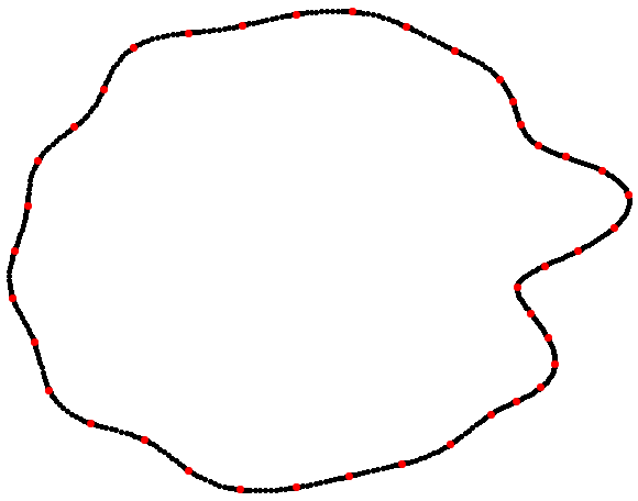 Figure 8: Test geometry for determining
2
4
6
8
5
5
15
20
Table 4: as a function of
Figure 8: Test geometry for determining
2
4
6
8
5
5
15
20
Table 4: as a function of
7.1 Maintaining Expansion Accuracy
The order of the multipole expansion in the FMM, , is dependent on the tree-level and frequency . Standard estimates are available for choosing this parameter for -expansions and -expansions (see, for example [12]). Briefly, the expansion order for an outgoing expansion is chosen to evaluate the sum
| (7.12) |
for in the far-field of the sources, with error less than . Suppose all the sources are contained in a box centered at the origin with , where is the size of the box at level . Using Graf’s addition theorem, the outgoing expansion associated with the box is given by
| (7.13) |
where
| (7.14) |
Here and are the polar coordinates of and respectively. The targets in the far-field of the box are are separated from box by at least one box length, i.e. . In order to compute the sum 7.12 with precision , the outgoing expansion is truncated at
| (7.15) |
if
| (7.16) |
In the QBX framework, the expansion order must be chosen to compute the sums
| (7.17) |
for all , and in the far-field of the sources, with error less than . Using Graf’s addition theorem, the outgoing expansion corresponding to the sum in Equation (7.17) is given by
| (7.18) |
where
| (7.19) |
Thus, outgoing expansion (7.18) can be truncated at if
| (7.20) |
for all . A similar analysis can be done for the incoming expansions as well.
While the above explanation provides an intuition for the need of larger outgoing and incoming expansions for the FMM-accelerated QBX as compared to the standard FMM, a detailed analysis for estimating is fairly involved. In the evaluation of the discretized layer potential , the far-field of the sum (7.17) is scaled by , where is a characteristic arc-length of a panel in the discretization of the boundary. Moreover, the size of the smallest box in the quad-tree data structure is also intricately tied to . Thus, we set and determine numerically, as a function of and , by testing the accuracy of the translated -expansions at targets close to the boundary for random geometries. The Helmholtz parameter was set to for these numerical experiments. The boundaries of the random test geometries were described by the following parametrization:
| (7.21) | ||||
| (7.22) |
where
| (7.23) |
where are uniformly distributed in and (see, Figure 8, for example).
In particular, analogous to the subsequent numerical experiments in Section 8.2, given and , we compute the relative error in Green’s identity for a known Helmholtz potential at a collection of targets close to the boundary. The associated layer potentials are evaluated using the FMM-accelerated QBX algorithm described in 7.2, and the geometry is sufficiently refined and over-sampled to ensure that the relative error in Green’s identity using a direct calculation is less than . The order of the multipole expansion in the FMM is set to , where we vary the parameter . The resulting is the minimum for which the relative error in Green’s identity computed using the FMM-accelerated QBX algorithm is less than . A contour plot of the error in evaluating the layer potential close to the boundary, wherein the local expansion coefficients are computed using a direct computation, and an FMM-accelerated QBX scheme for different values of is shown in Figure 9. The experiments indicated that was independent of the prescribed precision , and merely a function of . The results are summarized in Table 8


7.2 Complete Statement of the Fast Algorithm
To complement the previous discussion, and for mathematical and algorithmic completeness, we provide in this section a complete statement of the fast algorithm, including its ‘point’ and ‘layer potential’ parts, but excluding the geometry preprocessing described in detail earlier, with the differences to its prior ‘point-only’ version highlighted. Let be the smallest square centered at the origin which contains all sources, targets and expansion centers. Let be half the length of the side of the root-box square (its ‘radius’). Following the procedure described in Section 4.2, construct a quad-tree on .
In a minor abuse of notation, for any subset of the computational box, let , , and denote the set of sources, targets, and expansion centers contained in , respectively. Let be the highest level of refinement at any point.
A box is a parent box if it has been subdivided into one or more boxes.
A child box is a non-empty box resulting from the subdivision of a parent box.
Colleagues are adjacent boxes at the same level including the self-box. A given box has at most nine colleagues.
A leaf box is a childless box.
Let denote the coordinates of the center of box . Boxes and at level are well-separated from each other if
| (7.24) |
The -list of a box , denoted by , is empty if is a parent box. If is a leaf box, is the set of all leaf boxes that are adjacent to .
The -list of a box , denoted by , consists of all the children of the colleagues of the parent of that are well-separated from .
The far-field of a box will be denoted by .
The -list of a box , denoted by , is empty if is a parent box. If is a leaf box, consists of all the descendants of the colleagues of whose parents are adjacent to , but who are not adjacent to themselves. Note that a box is separated from by a distance equal to the length of the side of .
The -list of a box , denoted by , is formed by all boxes such that . Note that all boxes in the -list are childless and larger than .
Let denote the -term -expansion about the center of of the potential created by all sources in .
Let denote the -term -expansion about the center of box of the potential created by all sources in the far-field of , that is . The value is the result of evaluating the -expansion at target .
Let denote the -expansion about the center of representing the potential due to all sources .
Let denote the -expansion about the center of representing the potential due to all sources .
Let denote the potential at due to all sources .
Let denote the potential at due to all sources .
Let denote denote the -expansion coefficient at due to all sources .
Let denote the -expansion coefficient at due to all sources .
Let denote the -expansion coefficient
at due to all sources .
FMM-accelerated QBX
Comment [Choose main parameters]
| Given , using standard multipole estimates [24], set number of terms in expansions at level to . |
| Depending on , use Table 8 to determine and set . |
| Create a quad-tree on the computational domain containing all sources, targets, and expansion centers. |
| Choose the maximum number of particles in a childless box. |
| Subdivide a box if the sum of the number of sources and targets in is greater than . |
Comment [Refine the computational cell into a hierarchy of meshes.]
Stage 1.
| do | |||
| do | |||
| if contains more than particles then | |||
| subdivide into four boxes, ignore the empty boxes formed, add the non-empty boxes formed to . | |||
| end if | |||
| end do | |||
| end do |
Comment [Let denote the total number of boxes.]
Stage 2.
Comment [For every box at every level ,
form a multipole
expansion representing the potential outside due to all
the particles contained in .]
Comment [For each childless box , combine all charges inside to obtain the -expansion about the center of .]
| do | ||
| if is a childless box then | ||
| form a -term -expansion, representing the potential outside due | ||
| to all charges located in . | ||
| end do |
Comment [For each parent box , obtain the multipole expansion by translating the -expansions centered to an -expansion centered at , where is a child of . Add the resulting expansions together.]
| do | |||
| do | |||
| if is a parent box then | |||
| For each child of , shift the center of the -expansion to ’s center. | |||
| Add the resulting expansions together to obtain the expansion . | |||
| end if | |||
| end do | |||
| end do |
Stage 3.
Comment [For all particles in each childless box , compute the interactions with all sources directly.]
| do | ||
| if is childless then | ||
| For each target in , compute the sum of the interactions between and all sources . | ||
| New: For each expansion center in , compute the -expansion | ||
| coefficients, for , due to all sources . | ||
| end if | ||
| end do |
Stage 4.
Comment [For each box , convert
the -expansions of all boxes in into -expansions about
the center
of box .]
| do | ||
| do | ||
| Convert -expansion centered at into a -expansion centered at . | ||
| Add the resulting expansions to obtain . | ||
| end do | ||
| end do |
Stage 5.
Comment [For each childless box , evaluate the -expansions of all boxes in at every particle position in .]
| do | ||
| if is childless then | ||
| Evaluate the -expansion of each box to obtain for every target in . | ||
| New: Convert the -expansion of each box to obtain the -expansion | ||
| coefficients , for , for each expansion center . | ||
| end if | ||
| end do |
Stage 6.
Comment
[For each box , form local
expansions about the center representing the potential
due to all
sources .]
| do | |
| Convert the potential of all sources into a -expansion about the center of . | |
| end do |
Stage 7.
Comment [Shift the centers of -expansions of parent boxes to the centers of their children.]
| do | |||
| do | |||
| if is a parent box then | |||
| Shift the center of expansion to the center of each of ’s children . | |||
| Add the resulting expansion to . | |||
| end if | |||
| end do | |||
| end do |
Stage 8.
Comment [For each childless box , obtain as the sum of local expansions and . For each target in a childless box , evaluate and obtain the potential at by adding , and together.]
| do | ||
| if is childless then | ||
| Compute . | ||
| For each target in , evaluate . | ||
| Add , and to obtain the potential at . | ||
| New: For each expansion center in box , translate to compute -expansion | ||
| coefficients , about . | ||
| Add , and to obtain the -expansion coefficient at expansion center . | ||
| end if | ||
| end do |
8 Numerical Results
In the following subsections we illustrate the performance of FMM-accelerated QBX, both in terms of accuracy and speed. We demonstrate accuracy in evaluating layer potentials at targets both on the boundary and in the volume by verifying Green’s identity using known solutions to the Helmholtz equation. We also show the linear-time complexity of the algorithm described in Section 7.2, and compare its computational performance with timings for the underlying standard point-FMM. Finally, we use the Global QBX algorithm to solve a large multi-scale scattering problem with over 100,000 unknowns. All the experiments in this section are performed using a single core on a Dell laptop with a 2.2 GHz Intel Core i5-5200U processor and GB of RAM. The gfortran compiler, version 4.9.3, was used.
8.1 Preliminaries
For the Helmholtz parameter , let the boundary , , be parametrized as:
where the Fourier coefficients are listed in A. This parametrization traces a fish-like boundary, see Figure 10(a). Following the procedure described in [17], given a panel order , and a tolerance , we refine into piecewise panels, with the functions , on each panel interpolated using a -term Legendre polynomial expansions. The panels are refined until the each expansion and its requisite derivatives are resolved to the prescribed tolerance in a spectral -sense.
A typical test domain for all the numerical examples in this section is described here. Let be a collection of obstacles whose boundaries are up to an affine transformation, see Figure 10(b). Let , and denote the exterior of these obstacles.
Suppose satisfies the Helmholtz equation in along with the Sommerfeld radiation condition given by equations (1.1), and (1.3) respectively; then satisfies the Green’s identity
| (8.1) |
everywhere in . We verify this identity using QBX to evaluate the layer potentials and arbitrarily close to the boundary.


8.2 Accuracy and Complexity
Let be the Helmholtz potential generated by point sources placed inside the domains . The potential is then given by
where , and are randomly chosen. Obviously satisfies the homogeneous Helmholtz equation in , and therefore satisfies identity (8.1). To test the accuracy of the algorithm in 7.2, we compute the layer potentials , and obtain the error in (8.1) at targets on the boundary and in the exterior . Note that on the boundary, relationship (8.1) is interpreted in the one-sided limit as in (2.1). The targets in are identified using the algorithm described in Section 6.1.
Remark 3
For all of the numerical experiments, we use a level-restricted quad-tree for sorting sources, targets, and expansion centers in the computational domain. In a level-restricted quad-tree, two childless boxes which share a boundary point are no more than one level of refinement apart. There are several standard algorithms for converting a fully adaptive quad-tree into a level-restricted quad-tree and we implement the one discussed in [10].
Let and be the weighted relative-error in Green’s identity at the targets on the boundary and the volume, respectively:
and
Here is computed using QBX and is the Gaussian quadrature weight at the corresponding source on the boundary. Thus is a numerical approximation to the continuous relative error on the boundary:
We also analyze the performance of the algorithm for different combinations of , , and . The results are summarized in Tables 5 and 6. The first column is the tolerance requested in the algorithm. The second column is the order of Gauss-Legendre panels, given by . The third column is the QBX expansion order . Columns 4-7, denoted by , , , , are the number of discretization nodes on , the number of over-sampled nodes on , the number of targets, and the number of expansion centers, respectively. Columns 8-9, denoted by , , are the resolution of the single-layer density , and the double-layer density , respectively. Let denote the coefficients of the Legendre expansion of a function on panel . The resolution of the function , denoted , on the discretization of the geometry is then given by
| (8.2) |
where or depending on the panel order . The error is the maximum relative -norm of the tail of the Legendre expansion of scaled by the arclength of the panel. Column is for Table 5 and for Table 6. Finally, columns 11-13, denoted by , , , are the computation times. The time is the time required to evaluate the layer potential, is the time required for an with sources and targets, and is the time required for an FMM with sources and targets. A plot of the potential and errors in the Green’s identity test is given in Figure 11.


Remark 4
The difference between and is exactly the additional computational work in the FMM-accelerated QBX algorithm over the original FMM. The time , on the other hand, is the time required to apply an FMM on the original distribution of sources and targets.
| 5.00e-04 | 2 | 2 | 82536 | 330144 | 82536 | 82536 | 1.81e-04 | 7.49e-06 | 1.43e-03 | 11.71 | 4.24 | 2.00 |
| 165072 | 660288 | 165072 | 165072 | 6.85e-05 | 6.06e-06 | 1.53e-03 | 23.90 | 8.29 | 3.91 | |||
| 247608 | 990432 | 247608 | 247608 | 6.58e-05 | 1.75e-05 | 1.54e-03 | 37.65 | 12.78 | 6.02 | |||
| 330144 | 1320576 | 330144 | 330144 | 1.07e-04 | 1.04e-04 | 1.45e-03 | 48.67 | 17.04 | 8.07 | |||
| 5.00e-07 | 4 | 4 | 59328 | 296640 | 59328 | 59328 | 4.13e-06 | 1.52e-07 | 3.01e-07 | 15.28 | 5.73 | 2.27 |
| 118656 | 593280 | 118656 | 118656 | 2.28e-06 | 2.06e-07 | 3.06e-07 | 32.01 | 12.05 | 4.83 | |||
| 177984 | 889920 | 177984 | 177984 | 1.03e-06 | 6.69e-08 | 3.07e-07 | 46.87 | 17.48 | 7.26 | |||
| 237312 | 1186560 | 237312 | 237312 | 5.36e-06 | 1.90e-06 | 3.17e-07 | 61.44 | 22.00 | 9.10 | |||
| 5.00e-10 | 8 | 6 | 68544 | 342720 | 68544 | 68544 | 1.93e-10 | 9.49e-13 | 2.01e-10 | 36.38 | 9.35 | 3.92 |
| 137088 | 685440 | 137088 | 137088 | 3.24e-10 | 9.62e-13 | 6.22e-11 | 70.60 | 18.66 | 7.81 | |||
| 205632 | 1028160 | 205632 | 205632 | 2.91e-09 | 1.89e-12 | 1.78e-10 | 105.01 | 27.44 | 11.75 | |||
| 274176 | 1370880 | 274176 | 274176 | 3.51e-10 | 1.07e-12 | 1.00e-10 | 146.54 | 37.96 | 15.75 | |||
| 5.00e-13 | 16 | 8 | 76160 | 304640 | 76160 | 76160 | 4.19e-15 | 3.45e-16 | 3.79e-12 | 61.37 | 14.15 | 5.23 |
| 152320 | 609280 | 152320 | 152320 | 6.72e-15 | 1.03e-15 | 5.00e-12 | 118.22 | 26.96 | 10.80 | |||
| 228480 | 913920 | 228480 | 228480 | 1.13e-14 | 2.94e-15 | 4.02e-12 | 175.58 | 40.15 | 13.14 | |||
| 304640 | 1218560 | 304640 | 304640 | 8.76e-15 | 1.61e-15 | 6.36e-12 | 226.35 | 51.57 | 18.18 |
| 5.00e-04 | 2 | 2 | 55024 | 220096 | 550240 | 55024 | 1.24e-04 | 1.49e-06 | 2.13e-05 | 9.48 | 3.38 | 2.28 |
| 55024 | 220096 | 1100480 | 55024 | 1.24e-04 | 1.49e-06 | 1.74e-05 | 16.41 | 5.09 | 3.97 | |||
| 55024 | 220096 | 1650720 | 55024 | 1.24e-04 | 1.49e-06 | 1.61e-05 | 17.42 | 13.72 | 12.44 | |||
| 55024 | 220096 | 2200960 | 55024 | 1.24e-04 | 1.49e-06 | 1.68e-05 | 16.33 | 8.73 | 7.53 | |||
| 5.00e-07 | 4 | 4 | 59328 | 296640 | 593280 | 59328 | 4.13e-06 | 1.52e-07 | 1.99e-09 | 18.55 | 9.06 | 6.32 |
| 59328 | 296640 | 1186560 | 59328 | 4.13e-06 | 1.52e-07 | 8.53e-09 | 21.00 | 8.20 | 5.15 | |||
| 59328 | 296640 | 1779840 | 59328 | 4.13e-06 | 1.52e-07 | 2.41e-09 | 35.51 | 14.55 | 11.48 | |||
| 59328 | 296640 | 2373120 | 59328 | 4.13e-06 | 1.52e-07 | 2.69e-09 | 33.04 | 25.13 | 22.74 | |||
| 5.00e-10 | 8 | 6 | 58752 | 293760 | 587520 | 58752 | 1.49e-10 | 5.15e-13 | 1.13e-13 | 40.46 | 9.70 | 5.12 |
| 58752 | 293760 | 1175040 | 58752 | 1.49e-10 | 5.15e-13 | 1.06e-13 | 41.40 | 12.76 | 8.09 | |||
| 58752 | 293760 | 1762560 | 58752 | 1.49e-10 | 5.15e-13 | 9.56e-14 | 46.17 | 14.60 | 9.80 | |||
| 58752 | 293760 | 2350080 | 58752 | 1.49e-10 | 5.15e-13 | 1.19e-13 | 74.95 | 18.56 | 13.60 | |||
| 5.00e-13 | 16 | 8 | 60928 | 243712 | 609280 | 60928 | 4.80e-15 | 1.91e-16 | 1.20e-14 | 52.95 | 15.60 | 8.86 |
| 60928 | 243712 | 1218560 | 60928 | 4.80e-15 | 1.91e-16 | 3.21e-14 | 65.63 | 20.04 | 13.22 | |||
| 60928 | 243712 | 1827840 | 60928 | 4.80e-15 | 1.91e-16 | 2.74e-14 | 71.13 | 23.02 | 15.09 | |||
| 60928 | 243712 | 2437120 | 60928 | 4.80e-15 | 1.91e-16 | 2.45e-14 | 83.82 | 30.18 | 22.44 |
8.3 A scattering problem
Sound-soft scattering problems in acoustics correspond to exterior Dirichlet boundary value problems for the Helmholtz equation. Let , , denote the total potential, the incident potential and the scattered potential, respectively, all of which solve the homogeneous Helmholtz equation in the exterior region of a collection of obstacles except possibly at a finite number of points. Given an incident potential , the goal is to compute the scattered potential such that on the boundary , where denotes the boundary of the obstacles. Thus solves the exterior Helmholtz Dirichlet problem given by equations (1.1), (1.2), and (1.3), with Dirichlet data on the boundary .
Following the procedure described in the introduction, we represent the scattered potential as
| (8.3) |
where is an unknown density. On imposing the boundary conditions and using properties of the single- and double-layer potentials, we have the integral equation along :
| (8.4) |
We discretize the above equation using a Nyström method and use Global QBX for computing the layer potentials. Using the geometry discretization described in Section 8.1, consider the scattering problem in the exterior of inclusions discretized with -order Legendre expansions () and . Each panel is further subdivided once to ensure that the solution is well-resolved. Let be a plane-wave given by
| (8.5) |
where . On discretizing integral equation (8.4), we have a linear system with unknowns. We use an iterative GMRES-based solver to obtain the solution ; iterations are performed until we reach a relative residual of . The solution converged in iterations, the resolution of the density on the given discretization was , and the time required per iteration was sec. In Figure 12, we plot the real and imaginary parts of the resulting total potential .


9 Conclusions and future work
We have introduced a method for scalably performing singular quadrature using Quadrature by Expansion (QBX) within a fast algorithm based on the fast multipole method (FMM). The resulting algorithm is known as FMM-Accelerated Global QBX.
We have demonstrated that that the globally valid expansions of layer potentials necessary to carry out QBX can scalably be constructed using standard translation operators applied to - and -expansions. The resulting scheme scales like the underlying FMM in the low-frequency regime, with an asymptotic run time of , where is proportional to the number of sources in the discretization and targets in the volume. The constant implicit in the notation is only a small factor larger than that in the point-based FMM, roughly between two and four, depending on the desired precision.
Beyond merely providing a method for the evaluation of layer potentials, the scheme not only verifies a number of conditions required to guarantee its accuracy, it also automatically aids the user (by ways of mesh refinement) in ensuring that these conditions are met. We have thus obtained a capability to accurately evaluate layer potentials, scalably, anywhere in space, in a black-box fashion.
Under some circumstances, it is possible to construct algorithms that require less mesh refinement than the method presented here. This is particularly true in the case when some parts of the source geometry come so close to other parts that they almost touch each other. While the presented algorithm will provide an accurate answer case, it may not do so with the best possible efficiency. Motivated by these perspectives and the promising performance of the method presented here, a scheme denoted as Local QBX will be introduced in a subsequent paper [11] currently in preparation. This alternative scheme constructs expansions of the potential due to smaller pieces of the geometry, as necessary, in order to overcome extra geometry refinement.
Lastly, it is relatively straightforward to derive Global QBX schemes for computing layer potentials due to Stokeslets and stresslets in fluid dynamics, current and charge densities in electromagnetics, as well as other classical potentials in mathematical physics [23]. These, and extensions to three dimensions, are ongoing projects.
Acknowledgements
M. Rachh’s research was partially supported by the U.S. Department of Energy under contract DEFG0288ER25053 and by the Office of the Assistant Secretary of Defense for Research and Engineering and AFOSR under NSSEFF Program Award FA9550-10-1-0180. A. Klöckner’s research was supported by the National Science Foundation under grant DMS-1418961 and by the Office of the Assistant Secretary of Defense for Research and Engineering and AFOSR under NSSEFF Program Award FA9550-10-1-0180. M. O’Neil’s research was supported in part by the Office of the Assistant Secretary of Defense for Research and Engineering and AFOSR under NSSEFF Program Award FA9550-10-1-0180, and by the Office of Naval Research under Award N00014-15-1-2669. The authors would like to thank Leslie Greengard, Abtin Rahimian, and Matt Wala for several useful discussions.
The authors would further thank the anonymous referees for many helpful comments that led to a much-improved manuscript.
Appendix A Fourier coefficients for test geometry
| 0 | -3.03e-02 + i 0.00e+00 | -1.56e-02 + i 0.00e+00 |
|---|---|---|
| 1 | -1.00e-01 + i 2.34e-02 | -1.01e-02 - i 4.92e-02 |
| 2 | 1.28e-02 + i 2.16e-03 | -1.50e-03 + i 1.37e-02 |
| 3 | -9.40e-03 + i 3.98e-03 | 2.23e-04 - i 5.08e-03 |
| 4 | 3.18e-03 - i 1.92e-03 | -7.06e-03 - i 2.70e-03 |
| 5 | -3.42e-03 + i 3.37e-03 | -9.79e-03 + i 2.51e-03 |
| 6 | -2.13e-03 - i 3.87e-03 | -3.70e-03 + i 4.34e-03 |
| 7 | -4.24e-03 - i 3.45e-03 | -2.36e-03 - i 1.83e-03 |
| 8 | -1.61e-03 - i 2.24e-03 | 2.46e-03 - i 8.88e-04 |
| 9 | -1.32e-03 + i 1.85e-03 | 2.16e-03 - i 1.10e-04 |
| 10 | -4.06e-04 + i 2.52e-04 | -1.92e-03 - i 6.47e-04 |
| 11 | 5.58e-04 + i 6.41e-04 | -1.07e-03 - i 1.74e-04 |
| 12 | -1.29e-04 + i 1.88e-04 | -4.82e-05 - i 1.37e-04 |
| 13 | -8.71e-04 + i 1.47e-03 | -1.60e-03 - i 4.67e-05 |
| 14 | -5.12e-04 - i 1.51e-04 | 4.71e-04 - i 3.93e-04 |
| 15 | 4.31e-04 - i 4.82e-04 | 6.10e-04 + i 2.67e-04 |
| 16 | -3.51e-04 - i 5.28e-04 | -5.65e-04 + i 8.88e-04 |
| 17 | -7.72e-04 - i 2.93e-04 | -5.04e-04 - i 2.83e-04 |
| 18 | -3.65e-04 - i 2.33e-04 | 1.37e-04 - i 4.91e-04 |
| 19 | 8.68e-04 + i 3.97e-04 | 9.03e-05 + i 9.22e-05 |
| 20 | 1.50e-04 + i 1.72e-04 | -2.04e-04 - i 4.82e-05 |
| 21 | -2.22e-04 - i 1.72e-04 | -3.64e-04 - i 2.16e-04 |
| 22 | -3.09e-04 + i 2.04e-05 | -3.61e-04 + i 3.53e-05 |
| 23 | -1.92e-04 + i 2.53e-04 | -1.04e-04 - i 1.73e-05 |
| 24 | -3.36e-04 - i 1.48e-04 | 7.34e-05 + i 1.40e-04 |
| 25 | -1.16e-04 - i 6.38e-04 | 8.94e-05 - i 1.08e-04 |
| 26 | -2.24e-04 - i 1.73e-04 | 8.66e-05 - i 2.07e-05 |
|---|---|---|
| 27 | -5.47e-05 + i 2.16e-04 | 3.60e-05 - i 1.05e-04 |
| 28 | 9.47e-05 + i 3.04e-04 | -3.38e-04 + i 4.25e-06 |
| 29 | 1.87e-04 + i 7.48e-05 | -5.85e-05 - i 7.12e-05 |
| 30 | -6.42e-05 + i 2.08e-05 | -1.01e-04 - i 4.42e-05 |
| 31 | -2.33e-04 + i 2.49e-05 | -3.08e-05 + i 6.74e-05 |
| 32 | -1.47e-04 + i 7.06e-05 | 7.47e-05 + i 3.94e-05 |
| 33 | 3.51e-05 - i 1.69e-04 | -3.73e-05 - i 4.19e-06 |
| 34 | 4.50e-05 - i 1.88e-04 | -1.20e-04 + i 3.74e-05 |
| 35 | -9.51e-05 - i 1.18e-04 | -1.00e-05 - i 7.77e-05 |
| 36 | -8.54e-05 + i 7.05e-05 | -7.14e-05 - i 6.35e-05 |
| 37 | 9.22e-05 + i 9.62e-05 | -1.57e-05 - i 7.09e-05 |
| 38 | 1.07e-04 + i 5.55e-05 | 2.40e-05 - i 1.28e-04 |
| 39 | -5.84e-05 - i 5.48e-05 | -8.74e-05 + i 1.17e-04 |
| 40 | -1.58e-04 - i 4.45e-05 | -9.08e-05 + i 1.12e-05 |
| 41 | -1.31e-04 - i 2.73e-05 | 3.18e-05 - i 4.73e-05 |
| 42 | -6.19e-06 - i 2.10e-05 | 1.22e-04 + i 4.18e-05 |
| 43 | -8.43e-06 - i 7.75e-05 | -2.89e-05 + i 3.22e-05 |
| 44 | -5.35e-05 - i 2.64e-05 | -1.11e-04 - i 3.66e-05 |
| 45 | -2.68e-06 + i 1.33e-05 | -3.82e-05 - i 6.75e-05 |
| 46 | 4.99e-05 + i 1.14e-04 | -4.55e-05 - i 1.41e-05 |
| 47 | 6.65e-06 + i 4.98e-05 | -2.83e-05 - i 5.38e-05 |
| 48 | -2.05e-05 - i 6.93e-05 | -2.80e-05 - i 1.56e-05 |
| 49 | -2.32e-05 - i 6.10e-05 | 2.21e-05 + i 1.22e-05 |
| 50 | -2.31e-05 + i 3.32e-05 | 5.11e-05 + i 4.80e-05 |
References
References
- [1] M. Abramowitz and I. Stegun. Handbook of Mathematical Functions. Dover, 1965.
- [2] L. af Klinteberg and A.-K. Tornberg. Error estimation for quadrature by expansion in layer potential evaluation. Adv. Comput. Math., 2016. To appear.
- [3] A. Barnett. Evaluation of layer potentials close to the boundary for Laplace and Helmholtz problems on analytic planar domains. SIAM J. Sci. Comput., 36(2):A427–A451, 2014.
- [4] H. Brakhage and P. Werner. Über das Dirichletsche Außenraumproblem für die Helmholtzsche Schwingungsgleichung. Archiv der Mathematik, 16(1):325–329, 1965. doi: 10.1007/BF01220037.
- [5] J. Bremer, Z. Gimbutas, and V. Rokhlin. A nonlinear optimization procedure for generalized Gaussian quadratures. SIAM J. Sci. Comput., 32(4):1761–1788, 2010.
- [6] J. Carrier, L. Greengard, and V. Rokhlin. A Fast Adaptive Multipole Algorithm for Particle Simulations. SIAM J. Sci. Stat. Comput., 9(4):669–686, July 1988. doi: 10.1137/0909044.
- [7] D. Colton and R. Kress. Integral Equation Methods in Scattering Theory. John Wiley & Sons, Inc., 1983.
- [8] P. J. Davis and P. Rabinowitz. Methods of Numerical Integration. Academic Press, San Diego, 1984.
- [9] C. L. Epstein, L. Greengard, and A. Klöckner. On the convergence of local expansions of layer potentials. SIAM J. Num. Anal., 51(5):2660–2679, 2013.
- [10] J. F. Ethridge. Fast algorithms for volume integrals in potential theory. PhD thesis, New York University, 2000.
- [11] L. Greengard, A. Klöckner, and M. Rachh. Fast algorithms for Quadrature by Expansion II: Local expansions. In preparation.
- [12] L. Greengard, J. Huang, V. Rokhlin, and S. Wandzura. Accelerating fast multipole methods for the Helmholtz equation at low frequencies. IEEE Comput. Sci. Eng., 5(3):32–38, 1998.
- [13] R. B. Guenther and J. W. Lee. Partial Differential Equations of Mathematical Physics and Integral Equations. Dover, 1996.
- [14] S. Hao, A. H. Barnett, P.-G. Martinsson, and P. Young. High-order accurate Nystrom discretization of integral equations with weakly singular kernels on smooth curves in the plane. Adv. Comput. Math., 40:245–272, 2014.
- [15] J. Helsing. A fast and stable solver for singular integral equations on piecewise smooth curves. SIAM J. Sci. Comput., 33:153–174, 2011.
- [16] S. Jarvenpää, M. Taskinen, and P. Yla-Oijala. Singularity extraction technique for integral equation methods with higher order basis functions on plane triangles and tetrahedra. Int. J. Num. Meth. Eng., 58:1149–1165, 2003. doi: 10.1002/nme.810.
- [17] A. Klöckner, A. Barnett, L. Greengard, and M. O’Neil. Quadrature by expansion: A new method for the evaluation of layer potentials. J. Comput. Phys., 252:332–349, 2013.
- [18] R. Kress. Linear Integral Equations. Applied Mathematical Sciences, vol. 82, Springer, 1999.
- [19] E. Nyström. Über Die Praktische Auflösung von Integralgleichungen mit Anwendungen auf Randwertaufgaben. Acta Math., 54(1):185–204, 1930. doi: 10.1007/BF02547521.
- [20] F. W. J. Olver and National Institute of Standards and Technology (US). NIST Handbook of Mathematical Functions. Cambridge University Press, May 2010.
- [21] M. O’Neil, L. Greengard, and A. Pataki. On the efficient representation of the half-space impedance Green’s function for the Helmholtz equation. Wave Motion, 51:1–13, 2014.
- [22] O. I. Panich. On the solubility of exterior boundary-value problems for the wave equation and for a system of Maxwell’s equations. Uspekhi Matematicheskikh Nauk, 20(1):221–226, 1965.
- [23] A. Rahimian, A. Barnett, and D. Zorin. Ubiquitous evaluation of layer potentials using Quadrature by Kernel-Independent Expansion. 2016. arXiv:1612.00977 [math.NA].
- [24] V. Rokhlin. Rapid solution of integral equations of scattering theory in two dimensions. Journal of Computational Physics, 86(2):414–439, 1990.
- [25] N. Yarvin and V. Rokhlin. Generalized Gaussian quadratures and singular value decompositions of integral operators. SIAM J. Sci. Comput., 20:699–718, 1998.