The Lagrangian Deformation Structure of Three-Dimensional Steady Flow
Abstract
Fluid deformation and strain history are central to wide range of fluid phenomena ranging from mixing and particle transport to stress development in complex fluids and the formation of Lagrangian coherent structures (LCSs). To understand and model these processes it is necessary to quantify Lagrangian deformation in terms of Eulerian flow properties, currently an open problem. Whilst this problem has received much attention in the context of unsteady three-dimensional (3D) turbulent flow, there also exist several important classes of steady 3D flow such as chaotic, non-Newtonian and porous media flows. For steady 3D flows we develop a Protean (streamline) coordinate transform which renders both the velocity gradient and deformation gradient upper triangular. This frame not only simplifies computation of fluid deformation metrics such as finite-time Lyapunov exponents (FTLEs) and elucidates the deformation structure of the flow, but moreover explicitly recovers kinematic and topological constraints upon deformation evolution included those related to steady flow, helicity density and the Poincaré-Bendixson theorem. We apply this transform to several classes of steady 3D flow, including helical and non-helical, compressible and incompressible flows, and find random flows exhibit remarkably simple (Gaussian) deformation structure. As such this technique provides the basis for the development of stochastic models of fluid deformation in random flows which adhere to the kinematic constraints inherent to various flow classes.
I Introduction
Fluid deformation and strain history are central to wide range of fluid-borne phenomena, including fluid mixing and transport phenomena [39], identification of Lagrangian coherent structures and transport barriers [20], prediction of particle clustering or dispersion [4], alignment of material elements and scalar gradients [23], understanding and prediction of pair dispersion [37], and the development of stress in complex fluids [38]. In many of these applications, the ability to link Eulerian flow features such as the spatial velocity gradient to Lagrangian evolution of the deformation gradient tensor provides significant insights into the deformation structure of the flow. Whilst this problem is well-studied in the context of turbulent flows [18, 30, 22] there also exist several classes of steady 3D flow including chaotic and porous media flow which exhibit complex deformation behaviours. The steady nature of these flows imposes important constraints upon the evolution dynamics of both the velocity and deformation gradient tensors and so simplifies the link between flow structure and deformation. Such insights are of relevance to studies of fluid mixing, scalar dissipation or pair dispersion as they allow statistically quantified flow properties to be linked to evolution of fluid deformation which directly controls the associated fluid-borne phenomena. For example, in the context of fluid mixing, the distribution of Lagrangian fluid stretching rates serves as a quantitative input for lamellar mixing models [39, 40, 8, 26] based upon evolution and coalescence of concentration inhomogeneities which evolve as interacting lamellae. Similarly, the evolution of material surfaces and interfaces governs chemical reaction and front propagation. Whilst fluid deformation plays a pivotal role in these problems, it is often difficult to correlate Lagrangian deformation to Eulerian properties of the flow field. This is particularly challenging in the case of highly heterogeneous flow fields where perturbation methods are not appropriate.
Fluid deformation and strain history in non-Newtonian fluids controls the development of material stress and molecular or fibre orientation, and so is central to the constitutive modelling of complex fluids [41]. Many such constitutive models are posed in terms of a memory integral representation for the stress tensor [41], the solution of which can be very computationally intensive. Several works [6, 29, 33, 15] have devised Lagrangian numerical methods to alleviate the computational overhead associated with tracking and resolving particle trajectories and calculation of associated strain histories and convolutions thereof. This computational overhead is significantly reduced when the system is in transformed in streamline coordinates [14, 17], resulting in an upper triangular rate of strain tensor. For steady flows tracking of Lagrangian trajectories and free surface flows is greatly simplified as particles are confined to fluid streamlines [14]. This approach also simplifies calculation of fluid deformation and strain history, as the deformation gradient tensor admits closed-form solution consisting of a definite integrals evaluated along the streamline [2, 42]. This solution permits much more efficient calculation of both fluid deformation, strain history and associated convolutions.
Reorientation into streamline coordinates is also closely related to QR decomposition methods [12, 11] for accurate computation of Lyapunov exponents in continuous dynamical systems (posed as linear first order ODEs). This approach is based upon continuous decomposition of the fundamental solution matrix into orthogonal and upper triangular components which satisfy individual auxiliary evolution equations (ODEs) and possess beneficial qualities with respect to numerical approximation of Lyapunov spectra and adherence to constraints such as regularity and preservation of phase space. QR decomposition of 2 degree-of-freedom (d.o.f) autonomous linear first-order continuous dynamical systems is directly analogous to that of 2D fluid deformation in streamline coordinates, whereby the orthogonal matrix represents a rotation into the “streamline” coordinates of the dynamical system, and the upper triangular matrix is given by closed-form integrals of the reoriented systems along a “streamline”. Previously, QR decomposition methods have been considered as primarily numerical techniques for efficient and accurate computation, rather than to elucidate the governing dynamics and constraints of the dynamical system.
As such, reorientation of deformation evolution in 2D flows into streamline coordinates not only provides benefits with respect to numerical analysis, but also basic physical properties of the flow field (e.g. incompressibility, mass conservation) are naturally preserved by this formulation. Moreover, additional topological constraints associated with steady flow of continua (or autonomous continuous dynamical systems in general) are naturally recovered without need for ad-hoc enforcement. These constraints are particularly relevant as they directly limit evolution of the deformation gradient tensor.
One such constraint is imposed by the Poincaré-Bendixson theorem [36] which arises due to the fact that 1D streamlines cannot “cross” each other in a steady 2D flow. A direct consequence of this topological constraint is that fluid deformation in steady 2D flows on topologically simple manifolds can only grow at most algebraically in time. This constraint has important implications for the construction of models of fluid deformation in such flows, as naive implementations inherently generate exponential fluid stretching due to the homogeneous linear form of the temporal deformation evolution equation (6). Although sub-exponential stretching can be imposed via ad-hoc means such as the imposition of exponential waiting times between stretching events [39], such dynamics are not supported by experimental observations. To properly capture the underlying deformation dynamics, it is necessary that the modelling framework naturally recovers constraints on the deformation dynamics. Such constraints both simplify the modelling process and more clearly elucidate the role of flow structure in controlling fluid deformation.
Whilst the Poincaré-Bendixson theorem applies to 2D steady flow fields (or autonomous continuous dynamical systems on manifolds of zero topological genus in general), it also has significant implications for deformation in some steady 3D flows. As shown in [35, 34], flows with zero helicity density also must exhibit sub-exponential stretching as a consequence. The local helicity density introduced by Moffatt [31] is the product of the fluid velocity and vorticity
| (1) |
and the total helicity given by the volume integral over the closed flow domain is a measure of topological complexity of the flow field, related to the total knottedness of vortex lines within . There exist a wide class of zero helicity density flows, including all 2D flows; e.g. those defined by a Stokes streamfunction , , irrotational 2D and 3D flows in terms of the velocity potential , isotropic heterogeneous Darcy flow (where is the heterogeneous hydraulic conductivity), and toroidal flows where is the toroidal potential such as the Arter flow [21]. Note that in general tensorial Darcy flows have non-zero helicity density [43].
Spositio [35] shows that fluid streamlines in zero helicity density flows are confined to topologically simple 2D surfaces to which the Poincaré-Bendixson locally applies, enforcing sub-exponential fluid deformation under steady flow conditions. As per 2D steady flow, an appropriate modelling framework must enforce this constraint to avoid spurious non-physical behaviour. The use of streamline coordinates for steady 3D flows is analogous to the QR method for 3 d.o.f. systems, however in 3D the QR method does not necessarily conform to streamline coordinates and so does not recover these topological constraints. Such constraints not only have significant implications for models of fluid deformation in random flows, but also the fluid mechanics of complex fluids, as the rate of fluid stretching is integral to many constitutive models.
As outlined above, transformation into streamline coordinates in steady 2D flow greatly simplifies the evolution equations for the deformation tensor and recovers constraints upon the deformation dynamics. In this paper we extend this concept to steady 3D flows and uncover the deformation structure of several classes of such flows. Whilst streamline coordinates are unique in steady 2D flows, such a frame is not unique in steady 3D flows due arbitrary rotation of frame about a streamline, and do not necessarily render the transformed velocity gradient tensor upper triangular. In this study we develop a transform which aligns with 3D streamline coordinates and also renders the velocity gradient tensor upper triangular. Following Adachi [1] we term a system with these properties as a Protean coordinate system, which inherits the advantages of both the QR decomposition and streamline coordinate systems with respect to both numerical computation and physical insights into the dynamics which govern fluid deformation in 2D and 3D steady flows.
We present an alternative derivation to previous studies [1, 2, 5, 42] for the streamline coordinate transform into 2D flow, and then extend this to steady 3D flows to generate integral solutions of the full strain tensor. Whilst it was previously considered [5] that such analysis was too complex to be undertaken in 3D flow, we show this is possible for all steady 3D flow as the QR decomposition may be applied to all real square matrices.
Due to the simplicity of deformation evolution equation in the Protean frame, this transformation elucidates the link between Eulerian flow features and fluid deformation along Lagrangian trajectories and moreover, naturally enforces physical constraints upon deformation evolution. This structure naturally recovers the inherent kinematic and topological constraints associated with the Poincaré-Bendixson theorem and zero helicity flow, and so provides a framework for the development of a kinematically-consistent Continuous Time Random Walk (CTRW) model [10] of deformation in steady 3D flow. By way of example we apply this approach to a series of model flows, both compressible and incompressible, helical and non-helical and assess the numerical accuracy of the method and implications for understanding fluid deformation structure in complex 3D flows.
The remainder of the paper is organised as follows; in the following Section we briefly review the evolution of finite strain tensors in continuous media, and in Section III we consider objective transformation of the deformation gradient tensor into the Protean frame. We apply this transformation in Section IV to derive the core results for steady 2D flow via a more transparent route than previous studies, and then extend application to 3D flow in Section V. This method is then applied to the example flow classes in Section VI and concluding remarks are provided Section VIII.
II Evolution of Finite Strain Tensors
Fluid deformation and strain history are typically couched in terms of finite-strain tensors such as the right Cauchy-Green , left Cauchy-Green (Finger) , Green-Lagrangian and Hencky strain tensors [38], all of which are derived directly from the deformation gradient tensor , defined as
| (2) |
where are the respectively are reference material vectors in the Eulerian and Lagrangian frames. As such the deformation gradient tensor quantifies how the infinitesimal vector deforms from its reference state as . The evolution of an infinitesimal line element then evolves as
| (3) |
and similarly the the infinitesimal areal element spanned by the line elements , evolves as
| (4) |
an the fluid volume evolves as
| (5) |
Following the definition (2), the deformation gradient tensor evolves with travel time along a Lagrangian trajectory as
| (6) |
where the velocity gradient:= tensor , and the operator denotes differentiation along the Lagrangian trajectory .
The finite-strain tensors , , , , are all are objective (frame-indifferent) and hence provide appropriate strain measures for constitutive modelling [38] of non-Newtonian fluids. The stress-strain relationships for viscoelastic materials are often encoded via memory-integral constitutive models of the form [41]
| (7) |
where is the fluid stress, denotes historical time and represents a tensorial-valued functional which is dependant upon the entire strain history of the material. Explicitly, many memory integral equations are based upon convolution of the strain history with tensorial kernels which decay monotonically with increasing history , such as is given the Pipkin-Rogers (or similar) constitutive theory
| (8) |
In general, calculation of the stress evolution and general fluid mechanics of multidimensional viscoelastic flows via integral equations such as (8) can be very computationally expensive. Such computations may be significantly simplified via transformation of the deformation gradient into the Protean coordinate frame [42].
III Transformation of the Deformation Tensor into the Protean Frame
Whilst a formal description of fluid deformation in an arbitrary orthogonal curvilinear coordinate frame requires an excursion into differential geometry and tensor calculus, to clarify exposition and physical interpretation we consider transform of an orthogonal Cartesian coordinate system, and note that the formulation herein may be extended to general curvilinear coordinates via the standard tools of differential geometry. We denote spatial coordinates in the Cartesian coordinate system as , and the reoriented Protean (streamline) coordinate system by , such that the arbitrary velocity vector in the Cartesian frame transforms to in the Protean frame, where . These two frames are related by the local objective transform [38]
| (9) |
where is an arbitrary translation vector, and is a proper orthogonal transformation such as a rotation, hence and . The differential element transforms as
| (10) |
and from (2) the deformation tensor then transforms as
| (11) |
Whilst is often referred to as the deformation gradient tensor, it is not objective (as per (11), for some orthogonal matrix ), and so is not a tensor in the formal sense [38], however the finite strain tensors , , , are objective, and form a suitable basis for constitutive modelling. Differentiating (11) with respect to the Lagrangian travel time yields
| (12) |
where the transformed rate of strain tensor is then
| (13) |
and the contribution due to a moving coordinate frame is . As is orthogonal, then and so is skew-symmetric. From (10), the velocity vector also transforms as
| (14) |
The basic idea regarding use of Protean coordinates is to find an appropriate local reorientation to render the transformed velocity gradient upper triangular, yielding explicit solution of (12).
IV 2D Deformation Gradient Tensor in Protean Coordinates
In two spatial dimensions the reorientation matrix is then
| (15) |
and the basis vectors in the Protean frame are explicitly . The moving coordinate frame contribution may be expressed as
| (16) |
Note that , and since
| (17) |
for the travel time along a streamline, then the basis vector evolves with Lagrangian time as
| (18) |
and as the basis vectors , are orthogonal
| (19) |
Since , the elements of in (13) are then
| (20) |
and so
| (21) |
From (13), (16) the reoriented rate of strain tensor is then upper triangular:
| (22) |
Hence in two dimensional steady flow reorientation into Protean coordinates automatically renders the transformed velocity gradient tensor upper triangular. Note that this method is analogous to the continuous QR decomposition method for a –dimensional autonomous linear system, as outlined in Appendix A.
Due to the upper triangular form of , solution of the evolution equation (12) for the Protean deformation gradient tensor is particularly simple (via Gaussian elimination and the initial condition )
| (23) | ||||
| (24) | ||||
| (25) | ||||
| (26) |
For incompressible flow these expressions simplify to
| (27) | ||||
| (28) | ||||
| (29) | ||||
| (30) |
This result has previously been obtained by several workers [42, 1, 2, 5] to solve . As the reorientation matrix is known along a streamline, the Cartesian deformation tensor can then be directly calculated as .
The use of streamline coordinates in 2D steady continuous flow naturally imposes the topological constraints associated with these flows, namely that streamlines cannot cross on smooth 2D manifolds. In turn this constraint limits the rate of strain tensor along as streamline (17), as formalised by the Poincaré-Bendixson theorem. One implication of this theorem is that fluid stretching in steady 2D flow both parallel and transverse to the flow direction (quantified respectively by , ) must converge toward zero mean over long times for both incompressible and compressible flow. As such, the deformation components , cannot grow or decay without bound over long times. This is reflected by the explicit solution , where fluid stretching along the streamline coordinate is governed by fluctuations in the advective velocity . Similarly transverse stretching in incompressible flow is also bound as , and for compressible flow transverse stretching is limited by volumetric compression which must be finite due to mass conservation.
Therefore persistent fluid deformation in steady 2D flow can only arise via the off-diagonal term , and the solution for in (30) algebraic growth for as per the Poincaré-Bendixson theorem. From (22), the off-diagonal term = consists of contributions from shear deformation between streamlines and curvature of a streamline in the Protean frame. For open streamlines (and in particular flows such as Darcy and potential flows which do not admit closed streamlines [3]), the average of the curvature must average to zero over long times, whereas for closed streamlines, periodicity of the integral (30) yields fluid stretching which is linear in time. For flows which are ergodic in the Lagrangian sense (i.e. either mixing flows which admit ergodic particle trajectories or random flow fields), the long time average of the shear contribution must also have zero mean due to stationarity.
As the elongation of a material line is given by
| (31) |
then persistent fluid stretching in such flows arises from the fact that the elongation is governed by the absolute value of . In fact, episodes of low streamwise velocity add up to a strong increase of elongation as evidenced by the presence of in the denominator of the integrand in (30). The detailed link between transverse shear, velocity fluctuations and fluid deformation is studied by Dentz et al [9, 10], who show via a stretching continuous time random walk (CTRW) that the rate of fluid deformation in stationary random 2D steady flows can be modelled as a Lévy walk directly from these correlations. Hence the simple structure of the deformation gradient tensor in Protean coordinates clearly identifies the flow properties and constraints which govern fluid deformation.
V 3D Deformation Gradient Tensor in Protean Coordinates
V.1 Coordinate Reorientation in 3D Steady Flow
In contrast to steady 2D flow, the additional degree of freedom associated with steady 3D flow admits the possibility of chaotic Lagrangian dynamics. Specifically, steady flows with non-zero helicity density may exhibit chaotic dynamics and exponential fluid stretching due to relaxation of this topological constraint [31, 35]. In the Protean coordinate system, the base vector aligns with the velocity vector , such that , however the transverse vectors , are arbitrary up to a rotation about . As these base vectors are not necessary material coordinates, this gauge freedom does not impact the governing dynamics.
As per Section IV, it is desirable to reorient the rate of strain tensor such that it is upper triangular, yielding explicit closed-form solution for the deformation gradient tensor and elucidating the deformation dynamics. Whilst all square matrices are unitarily similar to an upper triangular matrix, it is unclear in general whether such a similarity transform is orthogonal, or corresponds to a reorientation of frame, or furthermore is a reorientation into streamline coordinates. This condition is satisfied for all steady 2D flows, but this is an open question for steady 3D flows.
Following the procedure for 2D flows, we begin by considering the 3D rotation matrix which reorients the Eulerian coordinate to the corresponding Protean coordinate which is tangent to the velocity vector . This reorientation is defined in terms of the rotation axis and angle which are given in terms of the local velocity vector and as
| (32) | ||||
| (33) |
and so
| (34) |
where denotes the cross product matrix of . Whilst reorientation via ensures the 1-coordinate in the Protean frame is always tangent to the velocity vector along a streamline, there exists a degree of freedom regarding orientation of the , coordinates in 3D flows. As such, we consider a further reorientation by an arbitrary angle about , such that the effective reorientation may be expressed as the composite
| (35) |
and is
| (36) |
The basis vectors in this reoriented frame are then
| (37) |
and so the 3D velocity gradient transforms as
| (38) |
Following (37), the moving frame contribution to is then
| (39) |
and these terms may be related to via the relations , , , yielding
| (40) | ||||
| (41) | ||||
| (42) |
| (43) |
and
| (44) |
As such, the component of is
| (45) |
and the rotated velocity gradient tensor is then
Similar to 2D steady flow and are both zero due to reorientation into the streamline frame, however in 3D flow in general. However, (V.1) shows that manipulation of the transverse orientation angle such that renders upper triangular, under the condition . From (38) the components of and are related as
| (49) | ||||
| (50) | ||||
| (51) |
and so the condition is then
| (52) |
where
| (53) | ||||
| (54) | ||||
| (55) |
V.2 Evolution of Protean Orientation Angle
Equation (52) describes a 1st-order ODE for the transverse orientation angle along a streamline which renders upper triangular, where the temporal derivative for is associated with both change in flow structure along a streamline and impact of a moving coordinate transform as encoded by . This is analogous to the ODE system (96) for the continuous QR method, with the important difference that the Protean reorientation gives a closed form solution for which constrains two degrees of freedom (d.o.f’s) for the Protean frame and an ODE for the remaining d.o.f characterised by , whereas the continuous QR method involves solution of the 3 degree of freedom ODE system (96), and requires unitary integrators to preserve orthogonality of . Similar to the 2D case, these methods differ with respect to the initial conditions , , where is given explicitly by (34), and is dependant upon as per (36), (52).
Whilst the ODE (52) admits an arbitrary initial condition which results in non-uniqueness of , this non-autonomous ODE is locally dissipative as reflected by the divergence
| (56) |
which admit maxima and minima of magnitude respectively at
| (57) |
Hence for , the ODE (52) admits an non-autonomous inertial manifold [32] , which exponentially attracts solutions from all initial conditions as illustrated in Fig. 1(a). As the inertial manifold is also a solution of (52), it may be expressed as , where is the initial condition on . Whilst all solutions of (52) render upper triangular, only solutions along the inertial manifold represent asymptotic dynamics independent of the initial condition , hence define the Protean frame as that which corresponds to the unique inertial solution .
| (a) | (b) |
As the inertial manifold maximises dissipation over long times, the associated initial condition is quantified by the limit
| (58) |
where
| (59) |
Whilst the inertial manifold can be identified by evolving (52) until acceptable convergence is determined, may be identified at shorter times via the approximation (59), as shown in Fig. 1(b). This approach is particularly useful when Lagrangian data is only available over short time-frames, and moreover explicitly identifies the inertial initial orientation angle , allowing the Protean transform to be applied from rather than the finite convergence time .
V.3 Protean Deformation in 3D Steady Flow
Given appropriate reorientation of the Protean frame given by (52) such that , the streamline velocity gradient tensor is upper triangular and from (12) is also upper triangular, with components
| (60) | ||||
| (61) | ||||
| (62) | ||||
| (63) | ||||
| (64) | ||||
| (65) |
The upper triangular form of simplfies solution of the components of the deformation tensor in that the integrals (62)-(65) can solved sequentially in a manner analogous to Gaussian elimination. Note that similar to 2D flow the streamwise deformation component simply oscillates as , and cannot grow over time. These dynamics are a direct consequence of the steady nature of the flow, whereas for unsteady flow the ensemble average of this component can change over time.
V.4 Protean Deformation in 3D Steady Zero Helicity Flow
For 3D steady zero helicity flows, constraints upon the flow structure further simplify both the dynamics of both the orientation angle and the deformation gradient evolution. Finnigan [17] demonstrates that all 3D flows with zero helicity density (or complex lamellar flows) may be expressed in the general form of an isotropic Darcy flow
| (66) |
with , where , , are smooth continuous functions which respectively represent hydraulic conductivity, velocity potential and streamfunction in isotropic Darcy flow. Such flow fields admit an orthogonal streamline coordinate system which comprise of material surfaces of constant streamfunction , isopotential surfaces of constant , and an additional material surface of constant normal to both of these. The velocity , vorticity and Lamb vectors are then normal to the isosurfaces of , , respectively.
Sposito [35, 34] identifies the stream surfaces of constant as Lamb surfaces [25] of the flow which are smooth non-intersecting 2D manifolds which are spanned by both streamlines and vorticity lines of the flow. These Lamb surfaces are both geometrically flat and topologically simple, comprising of either topological cylinders or tori [35, 34]. As such, the Poincaré-Bendixson theorem applies to streamlines, all of which are confined to these Lamb surfaces and so fluid deformation is restricted to grow algebraically in time. Conversely, streamlines in steady flows with non-zero helicity density do not conform to Lamb surfaces, and so may wander freely throughout the 3D flow domain and so may exhibit exponential fluid deformation.
In the material frame the velocity gradient tensor takes on a particularly simple form, and so we define the Protean coordinate frame for zero helicity density flows as this coordinate frame, such that the , coordinates align with the velocity and vorticity vectors respectively. Similar to 2D flow, the coordinate transform between the Cartesian and Protean frames is now explicit, consisting of the primary (34) and secondary (36) rotations, and is explicitly
| (67) |
where is the -th column vector of . Analysis of the differential geometry of this coordinate system in Appendix B shows that the material nature of this frame automatically renders the Protean velocity gradient tensor upper triangular. The analysis in Appendix B also shows that the constraints associated with zero helicity density flows render the transverse shear and vorticity components of the Protean velocity gradient tensor (114) to be zero
| (68) |
and so the components of the Protean deformation tensor then decouple as
| (69) |
As such the and ) components of the deformation tensor then simplify to
| (70) | ||||
| (71) |
where , represent longitudinal shear along surfaces of constant , respectively. Hence deformation in 3D zero helicity density flow evolves in a similar manner to that of 2D steady flow, where the only persistent deformation arises from shear and vorticity. This may be conceptualised as deformation due to 2D flow within a Lamb surface (), as well as contributions due to shear between Lamb surfaces (). This particularly simple deformation structure means that stochastic models of fluid deformation in steady 2D flows [10, 9] may be readily extended to steady 3D zero helicity flows.
VI Application to 3D Steady Flow
To illustrate utility of the method and uncover the deformation structure over a range of flows, we solve fluid deformation in the Protean frame over several classes of steady 3D flow summarised in Table 1. For all flows, particle trajectories from a random initial position are calculated to precision over the time period via an implicit Gauss-Legendre method. The associated deformation tensor in the Eulerian frame is calculated via solution of (6) to the same precision via the discrete QR decomposition method due to the large associated deformations. The Protean rate of strain tensor is then determined along these trajectories by solution of the inertial manifold in (52) via an explicit Runge-Kutta method over fixed time-steps (unless specified otherwise) and the Protean deformation gradient tensor is determined by direct evaluation of the integrals (60)-(63). We analyse the errors between the deformation tensor in the Cartesian and Protean frames, and calculate relevant measures of fluid deformation. For the deterministic ABC flow, statistics for the components of are computed over 1,000 particle trajectories from random initial locations within a chaotic region of the flow domain, whereas for the random flows the same statistics are gathered from a single trajectory over 1,000 realisations of the flow field.
| Flow/Property | Random | Helical | Compressible |
|---|---|---|---|
| ABC Flow | O | X | O |
| Kraichnan Flow | X | X | O |
| Dual Streamfunction Flow | X | X | O |
| Potential Flow | X | O | X |
VI.1 Arnol’d-Beltrami-Childress (ABC) Flow
 |
 |
| (a) | (b) |
We first apply the method to the Arnol’d-Beltrami-Childress (ABC) flow, an incompressible 3D Euler flow which is well-studied in the context of chaotic Lagrangian dynamics [13] . The ABC flow is a member of the class of Beltrami flows, with the property , hence the helicity density is non-zero throughout the triply-periodic flow domain , as given by the velocity field
| (72) |
We consider the parameter values , , used by Feingold [16] which generates chaotic trajectories over a subdomain of the global flow domain as illustrated by the space-filling particle trajectory shown in Fig. 2(a). Whilst the entire flow domain is not globally chaotic, we restrict attention to the deformation dynamics in the ergodic subdomain shown in Fig. 2. As the Lagrangian domain of chaotic flows are partitioned into topologically distinct chaotic and regular subdomains, relevant arguments regarding deformation dynamics in ergodic flows apply within each distinct chaotic (mixing) region. To study the deformation dynamics of this region and test the Protean method, we solve 1,000 particle trajectories over the period in this region and solve the Cartesian deformation tensor in (6) using a discrete QR decomposition method [11, 12], and compare these results with the Protean deformation tensor calculated directly from the integrals (62)-(65).
The impact of chaotic mixing along the trajectory in Fig. 2 is reflected by the rapid growth of the relative length of an infinitesimal () material line calculated via particle tracking shown in Fig. 3(a), which matches that calculated from the Protean deformation tensor as . Fig. 3(b) shows that the non-zero helicity density of the ABC flow imparts significant rotation to the transverse orientation angle along a particle trajectory. As the ABC flow is incompressible, the determinant of should equal unity for this flow, and the associated errors for the deformation gradient tensors are shown in Fig. 3(c)). As indicated by Fig. 3(d)), convergence between the principal stretching rate and the FTLE (84) is fairly rapid for this flow, however the FTLE approximation given by (90) converges significantly faster (as indicated by Figure 15).
| (a) | (b) |
| (c) | (d) |
To ascertain the accuracy of the coordinate transform as a function of the timestep , the quantities in Figure 3 are calculated over a range of time steps , , , , and the associated errors for the deformation tensor for these time steps are summarized in Figure 4 below. For all cases, the errors for are remarkably insensitive to the size of the time-step, indicating the coordinate transform is quite robust for all but the coarsest of time step . This timestep corresponds to spatial increments along particle trajectories which are of the order of the length-scale of the flow field, hence significant errors arising from cubic interpolation which impact estimation of both and . Hence the coordinate transform appears to be very stable so long as the spatial discretisation is sufficient to resolve the underlying flow features.
| (a) | (b) |
| (c) | (d) |
Probability density functions (PDFs) of the non-zero components of over 10,000 streamlines in the ergodic region of the ABC flow are shown in Figure 5, these correspond to spatial distributions throughout this region due to ergodicity. To within numerical precision, the diagonal components of this incompressible flow have mean stretching rates of , which agrees very favourably with the infinite-time Lyapunov exponent computed as .
The deformation structure in Figure 5(a) indicates that the velocity fluctuations associated with is highly peaked around zero, suggesting weak acceleration of the flow. Conversely, the transverse deformations , , are more broadly distributed throughout the ergodic region. Distributions of the off-diagonal components in Figure 5(b) indicate the stream-wise components , have zero mean, as is expected due to ergodicity. Conversely, the transverse component is consistently negative with mean -1.166, reflecting the strong helical component of Beltrami flows such as the ABC flow. In contrast with random ergodic flows, where will typically have zero mean due to stationary, this component may have non-zero mean as this chaotic flow is deterministic yet gives rise to ergodic trajectories.
| (a) | (b) |
We find the components of are all uncorrelated, with the exception of diagonal elements which are correlated as , , , a consequence of the volume-preserving nature of the ABC flow. The simplicity of the deformation structure of the ABC flow indicates the feasibility of developing stochastic models for evolution of the deformation tensor and FTLE PDFs. Whilst this development is beyond the scope of this study, these distributions above form the building blocks of such models, and clearly illustrate how the Eulerian flow features govern Lagrangian fluid deformation.
VI.2 3D Kraichnan Flow
 |
 |
| (a) | (b) |
We also apply the method to a 3D Kraichnan flow, a random model flow used extensively in the study of transport in homogeneous isotropic turbulence [24]. A variant of this incompressible flow with non-zero helicity density is given by the velocity field
| (73) |
where the 2D streamfunction is given by
| (74) |
and , are uniformly distributed independent random variables in and respectively and modes up to ==5 are used. A typical particle trajectory and the basic flow structure is shown in Figure 6. The Kraichnan flow possess non-zero helicity density and significant fluid stretching as per Figure 7(a), which consists of punctuated stretching events which lead to minimal persistent stretching. Rapid reorientation of the transverse angle driven by non-zero helicity density is reflected in Figure 7(b).
As shown in Fig 8, the deformation structure of the Kraichnan flow is particularly simple as all of the Protean rate of strain components are Gaussian distributed as a consequence of ergodicity and the Central Limit Theorem. Analysis of the normalized moments of all of these distributions indicate that all odd moments are statistically insignificant, and the 4th and 6th moments agree with those of a Gaussian distrubtion to within 10% and 20% respectively. The diagonal components and the off-diagonal components all appear to have the same variance, and the diagonal components have mean with , indicating significant exponential fluid stretching. Conversely, the off-diagonal components have zero mean, hence net fluid stretching arises from combination of these principal deformations and non-trivial correlations between the diagonal and off-diagonal stretching components. Similar to the ABC flow, all the components of are uncorrelated except for the diagonal components which are coupled as , , as consequence of incompressibility. This remarkably simple deformation structure of the 3D Kraichnan flow in Protean coordinates indicates that deformation in this flow can be fully characterised in terms of only a handful of parameters, hence it appears that prediction of the deformation tensor PDF is feasible via random walk models.
| (a) | (b) |
| (a) | (b) |
VI.3 Dual Stream Function Flow
 |
 |
| (a) | (b) |
Here we apply the Protean transform to a random 3D flow described by two stream functions. This incompressible flow with non-zero helicity density is given by the velocity field
| (75) |
where
| (76) |
and , are uniformly distributed independent random variables in and respectively, and modes up to ===5 are used. A typical particle trajectory and the basic flow structure is shown in Figure 9. As the stream functions and are invariants of the flow, streamlines are given by the intersection of level surfaces of , . Although this flow is helical and chaotic, fluid stretching is much smaller than the ABC or Kraichnan flows as per Figure 10(a), consisting of punctuated stretching events which lead to minimal persistent stretching. The rapid reorientation of transverse angle driven by non-zero helicity density is reflected in Figure 10(b).
Similar to the Kraichnan flow, the deformation structure of the dual streamfunction flow is particularly simple, consisting of Gaussian distributed Protean rate of strain components with the same variance amongst the diagonal and off-diagonal components. The off-diagonal components all have zero mean, with and having zero mean due to ergodicity, whilst has zero mean due to the random structure of the dual streamfunction flow. The diagonal components of have mean the form with significantly weaker exponential stretching exhibited as , again of similar magnitude to the Lyapunov exponent of the flow. As per the ABC and 3D Kraichnan flows, only the diagonal components of for the dual streamfunction flow are correlated due to incompressibility as , , .
| (a) | (b) |
| (a) | (b) |
VI.4 Random Potential Flow
 |
 |
| (a) | (b) |
Finally, we apply the Protean transform to the 3D random potential flow which is both compressible and irrotational, and so possesses identically zero helicity density. This flow is given by the superposed unidirectional and random velocity fields
| (77) |
where
| (78) |
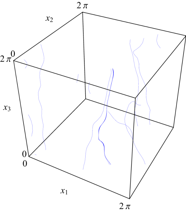
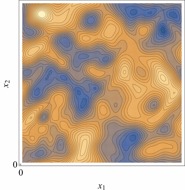
and , are uniformly distributed independent random variables in and respectively, and modes up to ===5 are used. The unidirectional background flow magnitude is set as . As per Figure 13(a), zero helicity density imparts much weaker algebraic fluid stretching. Note that whilst this flow is non-helical, as it is irrotational it does not admit Lamb surfaces, and so does not possess an orthogonal material coordinate system such as (99), and so the reoriented Protean coordinate system given by (1) for helical flows is used for this flow. Whilst the divergence of this flow has zero mean, particle trajectories are attracted to high density regions (where ), and likewise are repelled from low density regions. This bias causes particle trajectories to experience net compression in the Lagrangian frame, although the density- and flux-weighted average has zero mean by continuity. The non-helical nature of the flow imparts slow reorientation of the transverse angle as per Figure 13(b), which now only evolves in response to changes in the fluid structure.
Similar to the other random flows, the deformation structure of the 3D potential flow is particularly simple, consisting of Gaussian distributed Protean velocity gradient components with the same variance amongst the diagonal and off-diagonal components. Due to stationarity all of the off-diagonal components have zero mean, and zero helicity density everywhere ensures the diagonal components also all have zero mean. As such, the PDFs of the potential flow are completely characterised by two parameters; the variance of the diagonal and off-diagonal components. Similar to 2D steady random flows [10], persistent fluid stretching arises from correlations between the diagonal and off-diagonal components of , leading to algebraic fluid stretching. Again only the diagonal components of are correlated, however more weakly so due to the compressible nature of the flow: , , .
| (a) | (b) |
| (a) | (b) |
VII Discussion
Similar to 2D steady flows, reorientation into streamline coordinates yields explicit expressions for the deformation tensor as the series of integrals (62)-(65), and the eigenvalues of are simply the diagonal components . The explicit solution as is a direct consequence of the steady nature of the flow field. We define the temporal average of the principal deformation along a streamline with Lagrangian coordinate as
| (79) |
and the asymptotic limit as . The eigenvalues of are then = and for divergence-free flows . Due to conservation of mass, the expansion or compression of all fluid elements is bounded, hence for both compressible and incompressible flows, with the exception of streamlines which terminate at a stagnation point. As the -direction aligns with the mean fluid stretching then , and conversely in the 3-direction due to conservation of mass. For ergodic (mixing) flows such as turbulent, chaotic or random flows, the temporal average and the ensemble average both converge to a unique global average over the flow domain. Hence for ergodic steady 3D flows the set of average principal deformations may then be characterised in terms of a single parameter , where =.
As steady zero helicity density flows (but not necessarily flows with zero total helicity [21]) preclude chaotic dynamics [35], along all streamlines (irrespective of ergodicity), and the diagonal components grow sub-exponentially in time, . The Protean frame corresponding to the material coordinates naturally recovers this constraint of sub-exponential stretching as a direct consequence of the Poincaré-Bendixson theorem applied to Lamb surfaces of the flow, and the orientation angle in given explicitly as (67). Furthermore, as shown in Appendix B the transverse shear and vorticity in these flows is zero (, and so fluid deformation evolves longitudinally due to , in a manner analogous to 2D steady flow. This behaviour builds upon the insights discussed by Sposito [34, 35] regarding the deformation structure of isotropic Darcy flow, and shows that stochastic models of fluid deformation in such flows can be developed as a simple extension of those [10, 9] for steady 2D flows.
Steady 3D flows with non-zero helicity density exhibit Lagrangian chaos and exponential fluid stretching, and so converges to persistent non-zero values along streamlines, . Although the ensemble average of the Cartesian velocity gradient in random steady 3D flows converges toward zero due to statistical stationarity, persistent exponential stretching arises in these flows due to the asymmetry between fluid stretching and compression. Fluid stretching aligns material elements with the stretching direction, accentuating the stretching process, whereas compression aligns elements normal to the compression direction, retarding compression. This basic asymmetry leads to persistent exponential fluid stretching in random steady 3D flows, hence chaotic advection is the norm. This behaviour is not captured by the ensemble mean of the Cartesian velocity gradient , whereas in the Protean frame exponential stretching is directly quantified by the diagonal elements of .
Similar to the 2D case, in 3D ergodic flows the off-diagonal components of associated with the 1-coordinate have zero mean over long times due to cancellation of shear and streamline curvature over open particle trajectories. Conversely, the transverse off-diagonal component may have non-zero mean in ergodic (mixing) flows, but in random flows this transverse component must be zero due to stationarity. The mechanism leading to persistent fluid stretching in random zero helicity density flows () is the same as that for ergodic 2D flows described in Section IV.
For non-zero helicity density flows, the integrals (62)-(65) are significantly simplified by exponential growth and decay respectively of , . As the integrand in (64) decays as , then these converge to
| (80) | ||||
| (81) |
where the constant given by the integral in (64) is approximated as
| (82) |
As is bounded with zero mean, may be expressed as
| (83) |
where is an oscillatory function with non-zero mean . Note that these relationships hold both over a single trajectory or over an ensemble of trajectories in terms of the averages , if the relevant quantities are uncorrelated. For such chaotic flows is the dominant off-diagonal component of with respect to evolution of , where the full history of fluid shear and streamline curvature along a particle trajectory dictates , (which may be large in magnitude). In contrast is typically small and is only relevant at short times, and plays a negligible role in such flows.
An important measure with respect to fluid mixing, deformation and the formation of Lagrangian coherent structures (LCSs) is the finite-time Lyapunov exponent (FTLE) , which measures the exponential rate of fluid stretching as
| (84) |
where is the -th largest eigenvalue of the Cauchy-Green tensor along streamline with Lagrangian coordinate . For ergodic flows the corresponding infinite-time Lyapunov exponent
| (85) |
also converges to the ensemble average of due to ergodicity. In the presence of exponential fluid stretching, , in the asymptotic limit all the components of grow no faster than , and so the Lyapunov exponent is given the ensemble average of
| (86) |
providing a means to compute Lagrangian deformation from the Eulerian velocity gradient. From (86), the principal stretching rate converges toward the FTLE along a trajectory as
| (87) |
A more accurate approximation for the FTLE is provided by consideration of the full deformation tensor . As the sum of the singular values of (given by the eigenvalues of ) is equal to the Frobenius norm of
| (88) |
where for volume-preserving flows , then for large deformations the FTLE is well-approximated as
| (89) |
Hence the FTLE is well approximated by the dominant terms in the Frobenius norm over a single trajectory (labelled with Lagrangian coordinate ) or ensemble of trajectories respectively as
| (90) |
| (91) |
The accuracy of this approximation over both a single trajectory and an ensemble of 1,000 realisations of the Kraichnan flow (73) described in VI is illustrated in Figure 15. These results indicate that for all but short times (90), (91) accurately capture the finite-time stretching dynamics in the presence of significant exponential stretching. The offsets between the deformation components in Figure 15 are given by ensemble averages , , and the dominant FTLE is well approximated by (90), (91). As this approximation also holds over each trajectory, for ergodic flows (90) also facilitates estimation of both the FTLE and deformation tensor probability distribution function (PDF) given the statistics for , , .
| (a) | (b) |
VII.1 Stochastic Modelling of Lagrangian Deformation
It has been observed [27, 28, 7] that the Lagrangian velocities in several random 2D flows follow a spatial Markov process, facilitating quantification of transport in these flows as a continuous time random walk (CTRW) model. This remarkable property appears to also extend to the deformation structure of random 2D flows, where Dentz et al [10] have recently developed a CTRW model in the Protean frame to predict evolution of the PDF of as a Lévy process. This approach differs from other stochastic models [37, 39, 19] for fluid deformation in that the Protean transform directly provides the kernels for the deformation CTRW from the velocity gradient along streamlines, and automatically recovers topological and kinematic constraints inherent to the flow. This approach clearly elucidates the link between flow structure and deformation evolution and facilitate the identification of flow features which govern deformation. As such, the Protean transform provides a means to quantify the full deformation structure of complex ergodic steady 3D flows. As these flows exhibit Gaussian in terms of a small num
Extension of this CTRW deformation model to 3D steady flows facilitates prediction of the PDFs of Lagrangian deformation and the FTLE from the underlying Eulerian flow structure. We anticipate that this CTRW framework is applicable to a range of steady ergodic 3D flows, spanning non-zero helicity density flows such as chaotic flow fields, and zero helicity density flows such as heterogeneous Darcy flow. Such a development opens the door to prediction of fluid deformation from statistical flow features or the underlying material properties for flow in disordered media. Whilst establishment of spatial Markovianity and development of stochastic models is beyond the scope of this study, the simple deformation structure observed for the random flows in VI point to the feasibility of predict of the deformation PDF using such methods.
VIII Conclusions
We present an method to calculate fluid deformation in steady 3D flows using a Protean (streamline) coordinate system which renders the velocity gradient tensor upper triangular, facilitating explicit solution of the deformation gradient tensor in terms of definite integrals of the components of . Reorientation into Protean coordinates greatly simplifies computation of material deformation along particle trajectories, and naturally recovers physical, topological and kinematic constraints associated with the underlying flow field. These constraints such as the Poincaré-Bendixson theorem directly impact the dynamics of 3D fluid deformation as reflected by evolution of the deformation gradient tensor. Whilst this method is analogous to the continuous QR method, the QR method does not necessarily align with streamline coordinates. Similarly streamlines coordinate do not necessarily render upper triangular. Explicit reorientation in the Protean frame renders strict adherence to the above constraints, and moreover elucidates the underlying deformation structure and providing useful approximations for the finite- and infinite-time Lyapunov exponents, thus linking Lagrangian deformation with the Eulerian flow structure.
Although several models of fluid mixing require the mean (scalar) fluid deformation rate as an input, in general the full deformation tensor is required as this measure completely quantifies infinitesimal fluid deformation to first order at time . For example, the evolution of a continuously injected dye plume from a point or line source evolves in a different manner to that of a temporal pulse or indeed the area of a dye plume illuminated by a laser sheet transverse to the mean flow direction. Depending upon the situation at hand, these structures are governed by either the full deformation tensor or a subset of this measure. As such, quantification of the evolution of the deformation tensor can be applied to all of these cases, whereas scalar deformation measures are case-specific.
With respect to modelling of viscoelastic flows, solution of materials stress from strain history using a memory integral constitutive model is simplified in the Protean frame as the evolution of the fluid deformation gradient tensor (and hence associated Cauchy-Green , Finger or Hencky tensors) is given in closed form as integrals of the rate of strain tensor. This simplification also extends to solution of memory integral constitutive models for determining stress evolution in non-Newtonian (viscoelastic) materials, where the convolution of the entire strain history with a viscoelastic kernel is also significantly simplified.
This approach uncovers the deformation structure of a wide class of steady 3D flows, such that the link between compressibility, helicity density and stationarity and the components of are clearly elucidated. For zero helicity flows the Protean frame aligns with an orthogonal material coordinate system which recovers the inherent constraints of sub-exponential fluid deformation and zero transverse shear and vorticity. The resultant deformation structure is particularly simple, and may be considered as a generalisation of deformation in 2D shear flows.
For ergodic systems including random stationary flows or deterministic mixing flows, this approach points toward concrete methods to predict Lagrangian fluid deformation directly from the Eulerian flow structure whilst directly observing the constraints upon deformation evolution imposed by the underlying flow properties. This approach involves extension of a CTRW framework for 2D fluid deformation [10] to 3D flows, where the Eulerian PDF of and correlation between components serve as inputs to predict evolution of the PDF of the deformation tensor . This approach is particularly useful for developing stochastic models of deformation evolution in a wide class of ergodic flows including deterministic chaotic flows, random turbulent flows, or flow in disordered media, and in the latter case this approach opens the door to linking medium properties and statistical controls to deformation evolution.
We apply the Protean transformation method to several ergodic steady 3D flows, including model chaotic flow (ABC flow), isotropic homogeneous turbulence (Kraichnan model) and random potential flow, and demonstrate that the basic flow properties such as compressibility, helicity density and stationarity constrain the Protean rate of strain tensor as predicted and uncovers the underlying deformation structure of complex 3D flow fields, including prediction of the infinite-time Lyapunov exponent from finite-time data. The deformation structure of the random flows is remarkably simple (Gaussian) and completely uncorrelated apart from the diagonal components of which are correlated due to conservation of mass. These results provide the building blocks for the development of stochastic models of Lagrangian fluid deformation which observe relevant flow physics are relevant to fluid phenomena ranging from fluid mixing and transport through to particle dispersion and alignment.
Appendix A Analogy to Continuous QR Decomposition
As the Protean coordinate frame renders the transformed velocity gradient tensor upper triangular, this method is directly analogous to the continuous QR decomposition method for a -dimensional autonomous nonlinear dynamical system
| (92) |
which may be considered as the generalisation of the advection equation for a steady flow field. For a given solution trajectory , the Lyapunov exponents of (92) are given by the eigenvalues of the fundamental solutions of the linear variational equation
| (93) |
which is the generalisation of (6), where is the Jacobian along the trajectory . The continuous QR method considers the decomposition
| (94) |
where is orthogonal and upper triangular, and satisfy the auxiliary equations
| (95) | ||||
| (96) |
| (97) |
| (98) |
Hence the evolution equations for the orthogonal and upper triangular matrices , , for the continuous QR method are directly analogous to the reorientation operator , Protean rate of strain and Protean deformation gradient tensors for the Protean transform method. However, the actual values differ in that the initial condition for the QR method corresponds to the unrotated frame (), whereas the Protean frame always aligns with the flow direction as per (15). Due to the temporal derivative in the reoriented Jacobian (97) for the QR decomposition method, solutions to which render upper triangular are not unique.
Whilst asymptotically converges to the Protean coordinate frame (due to the dissipative nature of (96)), for finite times the continuous QR method does not align with the streamlines of the flow and hence inferences regarding topological and kinematic constraints upon the dynamics do not universally hold. Moreover, for 2D steady flows (and analogous dynamical systems), the Protean transform provides a simple closed solution (15) for , hence it is not necessary to explicitly solve the ODE system (96) or employ unitary integration routines [11] to preserve orthogonality of .
Appendix B Velocity Gradient Tensor in Zero Helicity Density Flow
As shown in [17, 35], all 3D zero helicity density flows may be posed in the form of an isotropic Darcy flow
| (99) |
where is the flow potential, the streamfunction and is a scalar, with . The streamsurfaces of constant are the Lamb surfaces of the flow, material surfaces which are spanned by both the velocity and vorticity vectors. Such zero helicity density flows admit an orthogonal material coordinate system which aligns with the stream lines, vorticity lines and Lamb vector field lines of the flow. In this frame the velocity gradient tensor takes on a particularly simple form, and so for zero helicity density flows we define this material frame as the Protean coordinate system. The covariant base vectors of this material coordinate system are then given by the normalised velocity, vorticity and Lamb vectors respectively as
| (100) |
Under this formulation the isopotential, stream and Lamb surfaces (respectively =const., const., const.) are all orthogonal and are normal to , , respectively. The orthogonal coordinates of the material coordinate system are then
| (101) | ||||
| (102) | ||||
| (103) |
where denote the distance along the coordinate . The differential arc length then satisfies , and the metric tensor for the orthogonal coordinate system is then
| (104) |
Note that as the components of the covariant and contravariant metric tensors transform as
| (105) | ||||
| (106) |
and as , then the scale factors are then
| (107) |
From the isotropic Darcy equation (99) and coordinate definitions (101)-(103) these scale factors are explicitly
| (108) | |||
| (109) | |||
| (110) |
where the local density of Lamb surfaces is defined as
| (111) |
Following Batchelor (1967), the components of the velocity gradient tensor are then
| (112) | ||||
| (113) |
hence the velocity gradient is upper triangular, and the components fully decouple as
| (114) |
where
| (115) | ||||
| (116) |
and the longitudinal shear rate and vorticity are respectively
| (117) | ||||
| (118) |
Hence fluid deformation in 3D steady flows with zero helicity density evolve in a similar manner to 2D steady flow due to longitudinal shear and vorticity within Lamb surfaces and stream surfaces. As these surfaces are material, there is no transverse shear in the directions, leading to decoupling as per (114).
References
- [1] K. Adachi. Calculation of strain histories in Protean coordinate systems. Rheologica Acta, 22(4):326–335, 1983.
- [2] K. Adachi. A note on the calculation of strain histories in orthogonal streamline coordinate systems. Rheologica Acta, 25(6):555–563, 1986.
- [3] J. Bear. Dynamics of Fluids in Porous Media. Number 1 in Dover Classics of Science and Mathematics. Dover, 1972.
- [4] Jérémie Bec, Massimo Cencini, Rafaela Hillerbrand, and Konstantin Turitsyn. Stochastic suspensions of heavy particles. Physica D: Nonlinear Phenomena, 237(14–17):2037 – 2050, 2008.
- [5] J.-R. Clermont and M.-E. de la Lande. Calculation of main flows of a memory-integral fluid in an axisymmetric contraction at high Weissenberg numbers. Journal of Non-Newtonian Fluid Mechanics, 46(1):89–110, 1993.
- [6] H. Court, A.R. Davies, and K. Walters. Long-range memory effects in flows involving abrupt changes in geometry part 4: Numerical simulation using integral rheological models. Journal of Non-Newtonian Fluid Mechanics, 8(1–2):95 – 117, 1981.
- [7] Pietro de Anna, Tanguy Le Borgne, Marco Dentz, Alexandre M. Tartakovsky, Diogo Bolster, and Philippe Davy. Flow intermittency, dispersion, and correlated continuous time random walks in porous media. Phys. Rev. Lett., 110:184502, May 2013.
- [8] Felipe P. J. de Barros, Marco Dentz, Jonas Koch, and Wolfgang Nowak. Flow topology and scalar mixing in spatially heterogeneous flow fields. Geophysical Research Letters, 39(8):n/a–n/a, 2012. L08404.
- [9] Marco Dentz, Tanguy Le Borgne, Daniel R. Lester, and Felipe P. J. de Barros. Scaling forms of particle densities for lévy walks and strong anomalous diffusion. Phys. Rev. E, 92:032128, Sep 2015.
- [10] Marco Dentz, Daniel R. Lester, Tanguy Le Borgne, and Felipe P. J. de Barros. Deformation in steady random flow is a Lévy walk. Phys. Rev. Lett., 2015.
- [11] Luca Dieci, Robert D. Russell, and Erik S. Van Vleck. On the compuation of Lyapunov exponents for continuous dynamical systems. SIAM Journal on Numerical Analysis, 34(1):402–423, 1997.
- [12] Luca Dieci and Erik S. Van Vleck. On the error in QR integration. SIAM Journal on Numerical Analysis, 46(3):1166–1189, 2008.
- [13] T. Dombre, U. Frisch, J. M. Greene, M. Hénon, A. Mehr, and A. M. Soward. Chaotic streamlines in the ABC flows. Journal of Fluid Mechanics, 167:353–391, 1986.
- [14] J.L. Duda and J.S. Vrentas. Fluid mechanics of laminar liquid jets. Chemical Engineering Science, 22(6):855 – 869, 1967.
- [15] K. Feigl and H.C. Öttinger. A numerical study of the flow of a low-density-polyethylene melt in a planar contraction and comparison to experiments. Journal of Rheology, 40(1):21–35, 1996.
- [16] Mario Feingold, LeoP. Kadanoff, and Oreste Piro. Passive scalars, three-dimensional volume-preserving maps, and chaos. Journal of Statistical Physics, 50(3-4):529–565, 1988.
- [17] J. J. Finnigan. A streamline coordinate system for distorted two-dimensional shear flows. Journal of Fluid Mechanics, 130:241–258, 5 1983.
- [18] S. S. Girimaji and S. B. Pope. Material-element deformation in isotropic turbulence. Journal of Fluid Mechanics, 220:427–458, 11 1990.
- [19] M. Gonzalez. Kinematic properties of passive scalar gradient predicted by a stochastic lagrangian model. Physics of Fluids, 21(5):–, 2009.
- [20] G. Haller. Distinguished material surfaces and coherent structures in three-dimensional fluid flows. Physica D: Nonlinear Phenomena, 149(4):248 – 277, 2001.
- [21] Darryl D. Holm and Yoshifumi Kimura. Zero-?helicity Lagrangian kinematics of three-?dimensional advection. Physics of Fluids A, 3(5):1033–1038, 1991.
- [22] A. S. Il’yn and K. P. Zybin. Material deformation tensor in time-reversal symmetry breaking turbulence. Physics Letters A, 379(7):650–653, 3 2015.
- [23] Patrice Klein, Bach Lien Hua, and Guillaume Lapeyre. Alignment of tracer gradient vectors in 2D turbulence. Physica D: Nonlinear Phenomena, 146(1–4):246 – 260, 2000.
- [24] Robert H. Kraichnan. Diffusion by a random velocity field. Physics of Fluids, 13(1):22–31, 1970.
- [25] H. Lamb. Hydrodynamics. The University Press, 1932.
- [26] T. Le Borgne, M. Dentz, and E. Villermaux. The lamellar description of mixing in porous media. Journal of Fluid Mechanics, 770:458–498, 5 2015.
- [27] Tanguy Le Borgne, Marco Dentz, and Jesus Carrera. Lagrangian statistical model for transport in highly heterogeneous velocity fields. Phys. Rev. Lett., 101:090601, Aug 2008.
- [28] Tanguy Le Borgne, Marco Dentz, and Jesus Carrera. Spatial markov processes for modeling lagrangian particle dynamics in heterogeneous porous media. Phys. Rev. E, 78:026308, Aug 2008.
- [29] David S. Malkus. Funtional derivatives and finite elements for the steady spinning of a viscoelastic filament. Journal of Non-Newtonian Fluid Mechanics, 8(3–4):223 – 237, 1981.
- [30] Charles Meneveau. Lagrangian dynamics and models of the velocity gradient tensor in turbulent flows. Annual Review of Fluid Mechanics, 43(1):219–245, 2011.
- [31] H. K. Moffatt. The degree of knottedness of tangled vortex lines. Journal of Fluid Mechanics, null:117–129, 1 1969.
- [32] Christian Pötzsche and Martin Rasmussen. Computation of nonautonomous invariant and inertial manifolds. Numerische Mathematik, 112(3):449–483, 2009.
- [33] J. Soulages, T. Schweizer, D.C. Venerus, M. Kröger, and H.C. Öttinger. Lubricated cross-slot flow of a low density polyethylene melt. Journal of Non-Newtonian Fluid Mechanics, 154(1):52–64, 2008.
- [34] Garrison Sposito. On steady flows with Lamb surfaces. International Journal of Engineering Science, 35(3):197 – 209, 1997.
- [35] Garrison Sposito. Topological groundwater hydrodynamics. Advances in Water Resources, 24(7):793 – 801, 2001.
- [36] G. Teschl. Ordinary Differential Equations and Dynamical Systems. Number 1 in Graduate studies in mathematics. American Mathematical Soc., 2012.
- [37] Simon Thalabard, Giorgio Krstulovic, and Jérémie Bec. Turbulent pair dispersion as a continuous-time random walk. Journal of Fluid Mechanics, 755, 9 2014.
- [38] C. Truesdell and W. Noll. The non-linear field theories of mechanics. Number v. 2 in The non-linear field theories of mechanics. Springer-Verlag, 1992.
- [39] E. Villermaux and J. Duplat. Mixing as an aggregation process. Phys. Rev. Lett., 91:184501, Oct 2003.
- [40] Stephen Wiggins and Julio M. Ottino. Foundations of chaotic mixing. Philosophical Transactions of the Royal Society of London. Series A: Mathematical, Physical and Engineering Sciences, 362(1818):937–970, 2004.
- [41] A. Wineman. Nonlinear viscoelastic solids—a review. Mathematics and Mechanics of Solids, 14(3):300–366, 2009.
- [42] H.H. Winter. Modelling of strain histories for memory integral fluids in steady axisymmetric flows. Journal of Non-Newtonian Fluid Mechanics, 10(1):157 – 167, 1982.
- [43] Yu Ye, Gabriele Chiogna, Olaf A. Cirpka, Peter Grathwohl, and Massimo Rolle. Experimental evidence of helical flow in porous media. Phys. Rev. Lett., 115:194502, Nov 2015.