跳到论文正文
W Papers独立论文阅读器 arXiv:1602.05268 论文正文 计算阅读时间 · 0%
引用这篇论文根据当前论文元数据生成,正式投稿前建议核对。


License: arXiv.org perpetual non-exclusive license
arXiv:1602.05268v1 [math.AP] 17 Feb 2016

Shape reconstruction of nanoparticles from their associated plasmonic resonancesThanks: This work was supported by the ERC Advanced Grant Project MULTIMOD–267184. Hai Zhang acknowledges a startup fund from HKUST.

Habib Ammari ††thanks: Department of Mathematics, ETH Zürich, Rämistrasse 101, CH-8092 Zürich, Switzerland (habib.ammari@math.ethz.ch, sanghyeon.yu@math.ethz.ch).    Mihai Putinar ††thanks: Department of Mathematics, University of California at Santa Barbara, Santa Barbara, CA 93106-3080, USA (mputinar@math.ucsb.edu), and School of Mathematics & Statistics, Newcastle University Newcastle upon Tyne, NE1 7RU, United Kingdom (mihai.putinar@ncl.ac.uk)    Matias Ruiz ††thanks: Department of Mathematics and Applications, Ecole Normale Supérieure, 45 Rue d’Ulm, 75005 Paris, France (matias.ruiz@ens.fr).    Sanghyeon Yu22footnotemark: 2    Hai Zhang ††thanks: Department of Mathematics, HKUST, Clear Water Bay, Kowloon, Hong Kong (haizhang@ust.hk).
Abstract

We prove by means of a couple of examples that plasmonic resonances can be used on one hand to classify shapes of nanoparticles with real algebraic boundaries and on the other hand to reconstruct the separation distance between two nanoparticles from measurements of their first collective plasmonic resonances. To this end, we explicitly compute the spectral decompositions of the Neumann-Poincaré operators associated with a class of quadrature domains and two nearly touching disks. Numerical results are included in support of our main findings.

Mathematics Subject Classification (MSC2000): 35R30, 35C20.

Keywords: plasmonic resonance, Neumann-Poincaré operator, algebraic domain, quadrature domain, nearly touching particles.

1 Introduction and main results

The present paper is a part of an ample and recent effort to understand the mathematical structure of inverse problems arising in nanophotonics. Although very classical, the spectral analysis of the Neumann-Poincaré operator emerges as the main theme of investigation.

Consider a domain Ω\Omega with 𝒞1,η\mathcal{C}^{1,\eta} boundary in ℝ2\mathbb{R}^{2} for η>0\eta>0. Let ν\nu denote the outward normal to ∂Ω\partial\Omega. Suppose that Ω\Omega contains the origin 00. For α=(α1,α2)∈ℕ2,\alpha=(\alpha_{1},\alpha_{2})\in\mathbb{N}^{2}, we denote by ∂α=∂1α1∂dα2\partial_{\alpha}=\partial_{1}^{\alpha_{1}}\partial_{d}^{\alpha_{2}} and α!=α1!​α2!\alpha!=\alpha_{1}!\alpha_{2}!.

The Neumann-Poincaré operator 𝒦Ω∗\mathcal{K}_{\Omega}^{*} associated with Ω\Omega is defined as follows:

𝒦Ω∗​[φ]​(x)=12​π​∫∂Ω⟨x−y,νx⟩|x−y|2​φ​(y)​𝑑σ​(y),x∈∂Ω.\mathcal{K}_{\Omega}^{*}[\varphi](x)=\frac{1}{2\pi}\int_{\partial\Omega}\frac{\langle x-y,\nu_{x}\rangle}{|x-y|^{2}}\varphi(y)d\sigma(y),\quad x\in\partial\Omega.

It is related to the single layer potential 𝒮Ω\mathcal{S}_{\Omega} given by

𝒮Ω​[φ]​(x)=12​π​∫∂Ωln⁡|x−y|​φ​(y)​𝑑σ​(y),x∈∂Ω,\mathcal{S}_{\Omega}[\varphi](x)=\frac{1}{2\pi}\int_{\partial\Omega}\ln|x-y|\varphi(y)d\sigma(y),\quad x\in\partial\Omega,

by the following jump relation:

(1.1) ∂𝒮Ω​[φ]∂ν|±\displaystyle\frac{\partial\mathcal{S}_{\Omega}[\varphi]}{\partial\nu}\Big|_{\pm} =(±12​I+𝒦Ω∗)​[φ]for ​φ∈L2​(∂Ω).\displaystyle=(\pm\frac{1}{2}I+\mathcal{K}_{\Omega}^{*})[\varphi]\quad\mbox{for }\varphi\in L^{2}(\partial\Omega).

It can be shown the operator λ​I−𝒦Ω∗:L2​(∂Ω)→L2​(∂Ω)\lambda I-\mathcal{K}_{\Omega}^{*}:L^{2}(\partial\Omega)\rightarrow L^{2}(\partial\Omega) is invertible for any |λ|>1/2|\lambda|>1/2. Furthermore, 𝒦Ω∗\mathcal{K}_{\Omega}^{*} is compact, can be symmetrized in a proper energy space and consequently its spectrum is discrete and contained in ]−1/2,1/2]]-1/2,1/2]; see for instance [8] for more details.

Using the quasi-static limit of electromagnetic fields, plasmonic resonances are associated with the set of eigenvalues λj\lambda_{j} of the Neumann-Poincaré operator 𝒦Ω∗\mathcal{K}_{\Omega}^{*} for which ⟨φj,xi⟩L2​(∂Ω)≠0\langle\varphi_{j},x_{i}\rangle_{L^{2}(\partial\Omega)}\neq 0, for either i=1i=1 or i=2i=2, where φj\varphi_{j} is an eigenfunction associated to λj\lambda_{j} [14, 15]. We refer the reader to [4, 7, 14, 15, 16, 17, 18, 21, 24, 30] for recent and interesting mathematical results on plasmonic resonances for nanoparticles.

In the present paper we prove that based on plasmonic resonances we can on one hand classify the shape of a class of domains with real algebraic boundaries and on the other hand recover the separation distance between two components of multiple connected domains. These results have important applications in nanophotonics. They can be used in order to identify the shape and separation distance between plasmonic nanoparticles having known material parameters from measured plasmonic resonances, for which the scattering cross-section is maximized [14, 15].

A real algebraic curve is the zero level set of a bivariate polynomial. Domains enclosed by real algebraic curves (henceforth simply called algebraic domains) are dense, in Hausdorff metric among all planar domains. On a simpler note, every smooth curve can be approximated by a sequence of algebraic curves. This observation turns algebraic curves into an efficient tool for describing shapes [20, 28, 32]. Note that an algebraic domain which is the sub level set of a polynomial of degree nn can uniquely be determined from its set of two-dimensional moments of order less than or equal to 3​n3n [22, 25]. In this paper we consider a class of algebraic curves determined via conformal mappings by two parameters mm and δ\delta, with mm being the order of the polynomial parametrizing the curve and δ\delta being a generalized radius, see (2.9). One can think of algebraic domains as non-generic, but dense, among all planar domains, as much as polynomials are non-generic, but dense among all continuous functions on a compact set. In either case, the identifications/reconstructions have to be complemented by a fine analysis of the rate of convergence.

The main results of the present paper are:

(i) Algebraic domains described by (2.9) have only two plasmonic resonances asymptotically (in δ\delta). Based on these two plasmonic resonances, one can classify them;

(ii) Two nearly touching disks have an infinite number of plasmonic resonances and the separating distance can be determined from the measurement of the first plasmonic resonance.

The paper is organized as follows. In section 2 we first introduce contracted generalized polarization tensors. Then we give explicit calculations of the Neumann-Poincaré operator associated with an algebraic domain. Moreover, we analyze its asymptotic behavior as δ\delta approaches zero. We compute the first- and second-order contracted polarization tensors, and show how to use them to determine the two parameters describing the algebraic boundaries. In section 3 we consider two nearly touching disks. We use the bipolar coordinates to compute the spectrum of the associated Neumann-Poincaré operator. We show that all the eigenvalues of the associated Neumann-Poincaré operator contribute to the set of plasmonic resonances. From the first-order polarization tensor, we show that we can recover the separating distance between the disks. In section 4 we illustrate our main findings in this paper with several numerical examples. In appendix A, we estimate the blow up of the gradient of the potential for two nearly touching disks at plasmonic resonances. This result generalizes to the plasmonic case, the estimates derived in [13, 11] for nearly touching disks with degenerate conductivities.

2 Plasmonic resonance for algebraic domains

2.1 Contracted generalized polarization tensors

Given a harmonic function HH in the whole plane, we consider the following transmission problem:

(2.1) {∇⋅(σΩ∇u)=0 in ​ℝ2,u−H=O⁡(|x|−1) as ​|x|→∞,\displaystyle\begin{cases}\nabla\cdot(\sigma_{\Omega}\nabla u)=0&\text{ in }\;\mathbb{R}^{2},\\[4.2679pt] u-H=O(|x|^{-1})&\text{ as }\;|x|\rightarrow\infty,\end{cases}

where σΩ=σ​χ​(Ω)+χ⁡(ℝ2\Ω¯)\sigma_{\Omega}=\sigma\chi(\Omega)+\chi(\mathbb{R}^{2}\backslash\overline{\Omega}) with σ>0\sigma>0, and χ⁡(Ω)\chi(\Omega) and χ⁡(ℝ2\Ω¯)\chi(\mathbb{R}^{2}\backslash\overline{\Omega}) are the characteristic functions of Ω\Omega and ℝ2\Ω¯\mathbb{R}^{2}\backslash\overline{\Omega}, respectively. From [10], we have

(2.2) u=H+𝒮Ω​(λ​I−𝒦Ω∗)−1​[∂H∂ν],\displaystyle u=H+\mathcal{S}_{\Omega}(\lambda I-\mathcal{K}_{\Omega}^{*})^{-1}[\frac{\partial H}{\partial\nu}]\,,

where

(2.3) λ=σ+12​(σ−1).\lambda=\frac{\sigma+1}{2(\sigma-1)}.

Decomposition (2.2) of uu together with

(2.4) H⁡(x)=∑α∈ℕd1α!​∂αH⁡(0)​xα\displaystyle H(x)=\sum_{\alpha\in\mathbb{N}^{d}}\frac{1}{\alpha!}\partial^{\alpha}H(0)x^{\alpha}

and

Γ⁡(x−y)=∑|β|=0+∞(−1)|β|β!​∂xβΓ⁡(x)​yβ,y​ in a compact set,|x|→+∞,\displaystyle\Gamma(x-y)=\sum_{|\beta|=0}^{+\infty}\frac{(-1)^{|\beta|}}{\beta!}\partial^{\beta}_{x}\Gamma(x)y^{\beta},\quad y\mbox{ in a compact set},\,|x|\rightarrow+\infty,

where Γ\Gamma is the fundamental solution to the Laplacian, yields the far-field behavior [10, p. 77]

(2.5) (u−H)​(x)=∑|α|,|β|≥11α!​β!​∂αH⁡(0)​[∫∂Ωyβ​(λ​I−𝒦Ω∗)−1​[∂xα∂ν]​(y)​𝑑σ​(y)]​∂βΓ⁡(x)\displaystyle(u-H)(x)=\sum_{|\alpha|,|\beta|\geq 1}\frac{1}{\alpha!\beta!}\partial^{\alpha}H(0)\bigg[\int_{\partial\Omega}y^{\beta}(\lambda I-\mathcal{K}_{\Omega}^{*})^{-1}[\frac{\partial x^{\alpha}}{\partial\nu}](y)d\sigma(y)\bigg]\;\partial^{\beta}\Gamma(x)

as |x|→+∞|x|\rightarrow+\infty. Introduce the generalized polarization tensors [10]:

Mα​β​(λ,Ω):=∫∂Ωyβ​(λ​I−𝒦Ω∗)−1​[∂xα∂ν]​(y)​𝑑σ​(y),α,β∈ℕd.M_{\alpha\beta}(\lambda,\Omega):=\int_{\partial\Omega}y^{\beta}(\lambda I-\mathcal{K}_{\Omega}^{*})^{-1}[\frac{\partial x^{\alpha}}{\partial\nu}](y)\,d\sigma(y),\qquad\alpha,\beta\in\mathbb{N}^{d}.

We call M:=Mα​βM:=M_{\alpha\beta} for |α|=|β|=1|\alpha|=|\beta|=1 the first-order polarization tensor.

For a positive integer mm, let Pm​(x)P_{m}(x) be the complex-valued polynomial

(2.6) Pm​(x)=(x1+i​x2)m:=∑|α|=maαm​xα+i​∑|β|=mbβm​xβ.P_{m}(x)=(x_{1}+ix_{2})^{m}:=\sum_{|\alpha|=m}a^{m}_{\alpha}x^{\alpha}+i\sum_{|\beta|=m}b^{m}_{\beta}x^{\beta}.

Using polar coordinates x=r​ei​θx=re^{i\theta}, the above coefficients aαma^{m}_{\alpha} and bβmb^{m}_{\beta} can also be characterized by

(2.7) ∑|α|=mamαxα=rmcosmθ, and ∑|β|=mbmβxβ=rmsinmθ.\sum_{|\alpha|=m}a^{m}_{\alpha}x^{\alpha}=r^{m}\cos m\theta,\text{ and }\sum_{|\beta|=m}b^{m}_{\beta}x^{\beta}=r^{m}\sin m\theta.

We introduce the contracted generalized polarization tensors to be the following linear combinations of generalized polarization tensors using the coefficients in (2.6):

Mm​nc​c=∑|α|=m∑|β|=naαm​aβn​Mα​β,Mm​nc​s=∑|α|=m∑|β|=naαm​bβn​Mα​β,\displaystyle M^{cc}_{mn}=\sum_{|\alpha|=m}\sum_{|\beta|=n}a^{m}_{\alpha}a^{n}_{\beta}M_{\alpha\beta},\quad M^{cs}_{mn}=\sum_{|\alpha|=m}\sum_{|\beta|=n}a^{m}_{\alpha}b^{n}_{\beta}M_{\alpha\beta},
Mm​ns​c=∑|α|=m∑|β|=nbαm​aβn​Mα​β,Mm​ns​s=∑|α|=m∑|β|=nbαm​bβn​Mα​β.\displaystyle M^{sc}_{mn}=\sum_{|\alpha|=m}\sum_{|\beta|=n}b^{m}_{\alpha}a^{n}_{\beta}M_{\alpha\beta},\quad M^{ss}_{mn}=\sum_{|\alpha|=m}\sum_{|\beta|=n}b^{m}_{\alpha}b^{n}_{\beta}M_{\alpha\beta}.

It is clear that

Mm​nc​c=∫∂Ωℜ⁡{Pn}​(λ​I−𝒦Ω∗)−1​[∂ℜ⁡{Pm}∂ν]​𝑑σ,\displaystyle M^{cc}_{mn}=\int_{\partial\Omega}\Re\{P_{n}\}(\lambda I-\mathcal{K}_{\Omega}^{*})^{-1}[\frac{\partial\Re\{P_{m}\}}{\partial\nu}]\,d\sigma,
Mm​nc​s=∫∂Ωℑ⁡{Pn}​(λ​I−𝒦Ω∗)−1​[∂ℜ⁡{Pm}∂ν]​𝑑σ,\displaystyle M^{cs}_{mn}=\int_{\partial\Omega}\Im\{P_{n}\}(\lambda I-\mathcal{K}_{\Omega}^{*})^{-1}[\frac{\partial\Re\{P_{m}\}}{\partial\nu}]\,d\sigma,
Mm​ns​c=∫∂Ωℜ⁡{Pn}​(λ​I−𝒦Ω∗)−1​[∂ℑ⁡{Pm}∂ν]​𝑑σ,\displaystyle M^{sc}_{mn}=\int_{\partial\Omega}\Re\{P_{n}\}(\lambda I-\mathcal{K}_{\Omega}^{*})^{-1}[\frac{\partial\Im\{P_{m}\}}{\partial\nu}]\,d\sigma,
Mm​ns​s=∫∂Ωℑ⁡{Pn}​(λ​I−𝒦Ω∗)−1​[∂ℑ⁡{Pm}∂ν]​𝑑σ.\displaystyle M^{ss}_{mn}=\int_{\partial\Omega}\Im\{P_{n}\}(\lambda I-\mathcal{K}_{\Omega}^{*})^{-1}[\frac{\partial\Im\{P_{m}\}}{\partial\nu}]\,d\sigma.

We refer to [8] for further details

As recently shown [2, 8, 9], the contracted generalized polarization tensors can efficiently be used for domain classification. They provide a natural tool for describing shapes. In imaging applications, they can be stably reconstructed from the data by solving a least-squares problem. They capture high-frequency shape oscillations as well as topology. High-frequency oscillations of the shape of a domain are only contained in its high-order contracted generalized polarization tensors.

The contracted generalized polarization tensors also satisfy simple invariance properties under translation, rotation, and scaling [2, 5]. Based on those properties, a dictionary matching algorithm can be developed. Assuming that the unknown shape of the target is an exact copy of some element from the dictionary, up to a rigid transform and dilatation, one can identify the target in the dictionary from its contracted generalized polarization tensors with a low computational cost [2]. If the material parameters of the domain are frequency dependent, then measurements taken at multiple frequencies allow very stable recognition of the targets. In [3], a classification approach based on the spectral properties of only the first-order polarization tensor was proposed and successfully implemented.

2.2 Algebraic domains of class 𝒬\mathcal{Q}

Let DD be the unit disk in ℂ\mathbb{C}. For m∈ℕm\in\mathbb{N} and a∈ℝa\in\mathbb{R}, define Φm,a:ℂ∖D¯→ℂ\Phi_{m,a}:\mathbb{C}\setminus\overline{D}\rightarrow\mathbb{C} by

Φm,a​(ζ)=ζ+aζm.\Phi_{m,a}(\zeta)=\zeta+\frac{a}{\zeta^{m}}.

Assume that Φm,a\Phi_{m,a} is injective on ℂ∖D¯\mathbb{C}\setminus\overline{D}. We introduce the class 𝒬\mathcal{Q} as the collection of all bounded domains Ω⊂ℂ\Omega\subset\mathbb{C} bounded by the curves

∂Ω={Φm,a(ζ):|ζ|=r0}for some r0>1,m∈ℕ and a∈ℝ.\partial\Omega=\{\Phi_{m,a}(\zeta):\quad|\zeta|=r_{0}\}\quad\mbox{for some }r_{0}>1,\quad m\in\mathbb{N}\mbox{ and }a\in\mathbb{R}.

Note that Φm,a\Phi_{m,a} is a conformal mapping from {|ζ|>r0}\{|\zeta|>r_{0}\} onto ℂ∖Ω¯\mathbb{C}\setminus\overline{\Omega}. In what follows, we shall suppress the subscript m,am,a from Φm,a\Phi_{m,a} for the ease of notation.

Conformal images of the unit disc by rational functions are also called quadrature domains. We refer to [23, 31] for details and ramifications of the theory of quadrature domains. In particular, up to the inversion z↦1/zz\mapsto 1/z, the complements of the domains in class 𝒬\mathcal{Q} are quadrature domains. We write for convenience ζ=eρ+i​θ\zeta=e^{\rho+i\theta}. Let ρ0\rho_{0} be such that r0=eρ0r_{0}=e^{\rho_{0}}. Let JJ be the Jacobian defined by

J=|∂ξ(Φ⁡(eξ))|ξ=ρ+i​θ|.J=\big|\partial_{\xi}\big(\Phi(e^{\xi})\big)|_{\xi=\rho+i\theta}\big|.

In the (ρ,θ)(\rho,\theta) plane, the normal derivative ∂/∂ν\partial/\partial\nu on ∂Ω\partial\Omega is represented as

∂∂ν=1J​∂∂ρ.\frac{\partial}{\partial\nu}=\frac{1}{J}\frac{\partial}{\partial\rho}.

Moreover, the boundary ∂Ω\partial\Omega is parametrized by

θ↦Φ⁡(eρ0+i​θ)=eρ0+i​θ+a​e−m​ρ0−i​m​θ.\theta\mapsto\Phi(e^{\rho_{0}+i\theta})=e^{\rho_{0}+i\theta}+ae^{-m\rho_{0}-im\theta}.

If we fix the constant aa and change ρ0\rho_{0}, then the size and the shape of ∂Ω\partial\Omega will change accordingly. In order to leave the shape unchanged, we need to represent the constant aa in a different way. We write

(2.8) a=e(m+1)​ρ0​δ.a=e^{(m+1)\rho_{0}}\delta.

Then the boundary ∂Ω\partial\Omega can be represented as

(2.9) θ↦Φ⁡(eρ0+i​θ)=eρ0​(ei​θ+δ​e−i​m​θ).\theta\mapsto\Phi(e^{\rho_{0}+i\theta})=e^{\rho_{0}}(e^{i\theta}+\delta e^{-im\theta}).

Now, if we fix the constant δ\delta and change ρ0\rho_{0}, then it is clear that only the size changes and the shape stays unaffected. The parameter eρ0e^{\rho_{0}} can be considered as a generalized radius of Ω\Omega because it determines the size. In conclusion, the shape of Ω\Omega is determined by the two parameters mm and δ\delta, while the size by the parameter ρ0\rho_{0}.

2.3 Explicit computation of the Neumann-Poincaré operator

In this section, we compute the Neumann-Poincaré operator on ∂Ω\partial\Omega explicitly. We need to compute 𝒦Ω∗​[J−1​cos⁡n​θ]\mathcal{K}^{*}_{\Omega}[J^{-1}\cos{n\theta}] and 𝒦Ω∗​[J−1​sin⁡n​θ]\mathcal{K}^{*}_{\Omega}[J^{-1}\sin{n\theta}] explicitly. Our strategy is as follows. Let u=𝒮Ω​[J−1​cos⁡n​θ]u=\mathcal{S}_{\Omega}[J^{-1}\cos{n\theta}] and v=𝒮Ω​[J−1​sin⁡n​θ]v=\mathcal{S}_{\Omega}[J^{-1}\sin n\theta]. If u,vu,v can be obtained explicitly, then 𝒦Ω∗​[J−1​cos⁡n​θ]\mathcal{K}^{*}_{\Omega}[J^{-1}\cos{n\theta}] and 𝒦Ω∗​[J−1​sin⁡n​θ]\mathcal{K}^{*}_{\Omega}[J^{-1}\sin{n\theta}] are immediately derived by using the following identity:

(2.10) 𝒦Ω∗​[φ]=12​(∂𝒮⁡[φ]∂ν|++∂𝒮⁡[φ]∂ν|−),\mathcal{K}^{*}_{\Omega}[\varphi]=\frac{1}{2}\bigg(\frac{\partial\mathcal{S}[\varphi]}{\partial\nu}\Big|_{+}+\frac{\partial\mathcal{S}[\varphi]}{\partial\nu}\Big|_{-}\bigg),

which follows from (1.1). For simplicity, we consider only uu. By using the continuity of the single layer potential and the jump relation (1.1), we can see that the function uu is the solution to the following problem:

(2.11) {Δ​u=0 in ​ℂ∖∂Ω,u|−=u|+ on ​∂Ω,∂u∂ν|+−∂u∂ν|−=J−1​cos⁡n​θ on ​∂Ω,u=O⁡(|z|−1) as ​|z|→∞.\ \left\{\begin{array}[]{ll}\displaystyle\Delta u=0&\mbox{ in }\mathbb{C}\setminus\partial{\Omega},\\[5.0pt] \displaystyle u|_{-}=u|_{+}&\mbox{ on }\partial\Omega,\\[5.0pt] \displaystyle\frac{\partial u}{\partial\nu}\Big|_{+}-\frac{\partial u}{\partial\nu}\Big|_{-}=J^{-1}\cos{n\theta}&\mbox{ on }\partial\Omega,\\[10.00002pt] \displaystyle u=O(|z|^{-1})&\mbox{ as }|z|\rightarrow\infty.\end{array}\right.

Let u~​(ρ,θ)=(u∘Φ)​(eρ+i​θ)\widetilde{u}(\rho,\theta)=(u\circ\Phi)(e^{\rho+i\theta}). Since Φ⁡(ζ)\Phi(\zeta) is conformal on |ζ|>eρ0|\zeta|>e^{\rho_{0}}, the above problem can be rewritten as follows:

(2.12) {Δ​u=0 in  for ​ρ<ρ0,Δ​u~=0 for ​ρ>ρ0,u~|−=u~|+ on ​ρ=ρ0,∂u~∂ρ|+−∂u~∂ρ|−=cos⁡n​θ on ​ρ=ρ0,u~=O⁡(e−ρ) as ​ρ→∞.\ \left\{\begin{array}[]{ll}\displaystyle\Delta u=0&\mbox{ in }\mbox{ for }\rho<\rho_{0},\\[5.0pt] \displaystyle\Delta\widetilde{u}=0&\mbox{ for }\rho>\rho_{0},\\[5.0pt] \displaystyle\widetilde{u}|_{-}=\widetilde{u}|_{+}&\mbox{ on }\rho=\rho_{0},\\[5.0pt] \displaystyle\frac{\partial\widetilde{u}}{\partial\rho}\Big|_{+}-\frac{\partial\widetilde{u}}{\partial\rho}\Big|_{-}=\cos{n\theta}&\mbox{ on }\rho=\rho_{0},\\[10.00002pt] \displaystyle\widetilde{u}=O(e^{-\rho})&\mbox{ as }\rho\rightarrow\infty.\end{array}\right.

Note that in (2.12), the first equation for u|Ωu|_{\Omega} is not represented in terms of u~\widetilde{u}. This is due to the singularity of Φ⁡(ζ)\Phi(\zeta) near ζ=0\zeta=0. Hence, we need to consider u|Ωu|_{\Omega} more carefully. If a=1a=1 and m=1m=1, then Ω\Omega becomes an ellipse and (ρ,θ)(\rho,\theta) are called the elliptic coordinates. In this case, equation (2.12) for u~\widetilde{u} can be easily solved by imposing some appropriate conditions on ρ=ρ0\rho=\rho_{0} and ρ=0\rho=0. However, for general shaped domains, this is not easy.

Fortunately, we can overcome this difficulty by the fact that the shape of the domain Ω\Omega is defined by a rational function Φ⁡(ζ)=ζ+a/ζm\Phi(\zeta)=\zeta+a/\zeta^{m}. Our strategy is to seek a solution to (2.12) such that

u⁡(z)=ℜ⁡{a polynomial of degree n in z}for ​z∈Ω.u(z)=\Re\{\mbox{a polynomial of degree $n$ in $z$}\}\quad\mbox{for }z\in\Omega.

We can show that, for 1≤n≤m1\leq n\leq m, u|Ωu|_{\Omega} in equation (2.12) can be explicitly solved by using the following ansatz:

u|Ω​(z)∝ℜ⁡{zn}\displaystyle u|_{\Omega}(z)\propto\Re\{z^{n}\} =ℜ⁡{(ζ+aζm)n}\displaystyle=\Re\Big\{\Big(\zeta+\frac{a}{\zeta^{m}}\Big)^{n}\Big\}
=ℜ∑k=0n(nk)ζn−k(aζm)k(ζ=eρ​I​θ)\displaystyle=\Re\sum_{k=0}^{n}\begin{pmatrix}n\\ k\end{pmatrix}\zeta^{n-k}\Big(\frac{a}{\zeta^{m}}\Big)^{k}\qquad(\zeta=e^{\rho I\theta})
(2.13) =en​ρcosnθ+∑k=1nak(nk)e−tkm​n​ρcostm​nkθ,\displaystyle=e^{n\rho}\cos n\theta+\sum_{k=1}^{n}a^{k}\begin{pmatrix}n\\ k\end{pmatrix}e^{-t^{mn}_{k}\rho}\cos t^{mn}_{k}\theta,

where the constant tkm​nt^{mn}_{k} is defined by

tkm​n=(m+1)​k−n,0≤k≤n.t_{k}^{mn}=(m+1)k-n,\quad 0\leq k\leq n.

As will be seen later, for the purpose of computing the polarization tensor, we consider only the case where 1≤n≤m1\leq n\leq m. (If n>mn>m, u|Ω​(z)u|_{\Omega}(z) turns out to be more complicated polynomial than znz^{n} but is still a polynomial of degree nn.)

Let us assume 1≤n≤m1\leq n\leq m. In view of (2.13), we define

w⁡(ρ,θ):\displaystyle\displaystyle w(\rho,\theta): ={en​ρcosnθ+∑k=1nak(nk)e−tkm​n​ρcostm​nkθ,ρ<ρ0,e−n⁡(ρ−2​ρ0)cosnθ+∑k=1nak(nk)e−tkm​n​ρcostm​nkθ,ρ>ρ0.\displaystyle=\begin{cases}\displaystyle e^{n\rho}\cos n\theta+\sum_{k=1}^{n}a^{k}\begin{pmatrix}n\\ k\end{pmatrix}e^{-t^{mn}_{k}\rho}\cos t^{mn}_{k}\theta,&\quad\rho<\rho_{0},\\[15.00002pt] \displaystyle{e^{-n(\rho-2\rho_{0})}}\cos n\theta+\sum_{k=1}^{n}a^{k}\begin{pmatrix}n\\ k\end{pmatrix}e^{-t^{mn}_{k}\rho}\cos t^{mn}_{k}\theta,&\quad\rho>\rho_{0}.\end{cases}

Note that ww is harmonic in {ρ<ρ0}\{\rho<\rho_{0}\} and {ρ>ρ0}\{\rho>\rho_{0}\} and w=O⁡(e−ρ)w=O(e^{-\rho}) as ρ→∞\rho\rightarrow\infty. Moreover,

(2.14) {w|+=w|− on ​ρ=ρ0,∂w∂ρ|+−∂w∂ρ|−=(−2)​n​en​ρ0​cos⁡n​θ on ​ρ=ρ0.\displaystyle\begin{cases}\displaystyle w|_{+}=w|_{-}&\quad\mbox{ on }\rho=\rho_{0},\\[5.0pt] \displaystyle\frac{\partial w}{\partial\rho}\Big|_{+}-\frac{\partial w}{\partial\rho}\Big|_{-}=(-2)ne^{n\rho_{0}}\cos n\theta&\quad\mbox{ on }\rho=\rho_{0}.\end{cases}

Therefore, the function ww is equal to u~\widetilde{u} up to a multiplicative constant. More precisely, we have

(2.15) u~​(ρ,θ)=−12​n​e−n​ρ0​w​(ρ,θ).\widetilde{u}(\rho,\theta)=-\frac{1}{2n}e^{-n\rho_{0}}w(\rho,\theta).

Now we are ready to compute 𝒦Ω∗​[J−1​cos⁡n​θ]\mathcal{K}_{\Omega}^{*}[J^{-1}\cos n\theta]. We can check that

(2.16) 12​(∂w∂ρ|ρ=ρ0++∂w∂ρ|ρ=ρ0−)\displaystyle\frac{1}{2}\bigg(\frac{\partial w}{\partial\rho}\Big|^{+}_{\rho=\rho_{0}}+\frac{\partial w}{\partial\rho}\Big|^{-}_{\rho=\rho_{0}}\bigg) =∑k=1n−tm​nkak(nk)e−tkm​n​ρ0costm​nkθ.\displaystyle=\sum_{k=1}^{n}-t^{mn}_{k}a^{k}\begin{pmatrix}n\\ k\end{pmatrix}e^{-t^{mn}_{k}\rho_{0}}\cos t^{mn}_{k}\theta.

Then it follows from (2.10) and (2.15) that

(2.17) 𝒦Ω∗[J−1cosnθ]=1J∑k=1nδktkm​n2​n(nk)costkm​nθ\mathcal{K}_{\Omega}^{*}[J^{-1}\cos n\theta]=\frac{1}{J}\sum_{k=1}^{n}\delta^{k}\frac{t^{mn}_{k}}{2n}\begin{pmatrix}n\\ k\end{pmatrix}\cos t^{mn}_{k}\theta

for 1≤n≤m1\leq n\leq m. In exactly the same manner, we can show that

(2.18) 𝒦Ω∗[J−1sinnθ]=−1J∑k=1nδktkm​n2​n(nk)sintkm​nθ.\mathcal{K}_{\Omega}^{*}[J^{-1}\sin n\theta]=-\frac{1}{J}\sum_{k=1}^{n}\delta^{k}\frac{t^{mn}_{k}}{2n}\begin{pmatrix}n\\ k\end{pmatrix}\sin t^{mn}_{k}\theta.

It is worth mentioning that we can also compute the single layer potentials for J−1​cos⁡n​θJ^{-1}\cos n\theta and J−1​sin⁡n​θJ^{-1}\sin n\theta:

(2.19) 𝒮Ω​[J−1​cos⁡n​θ]\displaystyle\mathcal{S}_{\Omega}[J^{-1}\cos n\theta] =−12​ncosnθ−12​n∑k=1nδk(nk)costm​nkθ,\displaystyle=-\frac{1}{2n}\cos n\theta-\frac{1}{2n}\sum_{k=1}^{n}\delta^{k}\begin{pmatrix}n\\ k\end{pmatrix}\cos t^{mn}_{k}\theta,

and

(2.20) 𝒮Ω​[J−1​sin⁡n​θ]\displaystyle\mathcal{S}_{\Omega}[J^{-1}\sin n\theta] =−12​nsinnθ+12​n∑k=1nδk(nk)sintm​nkθ.\displaystyle=-\frac{1}{2n}\sin n\theta+\frac{1}{2n}\sum_{k=1}^{n}\delta^{k}\begin{pmatrix}n\\ k\end{pmatrix}\sin t^{mn}_{k}\theta.

2.4 Asymptotic behavior of the Neumann-Poincaré operator 𝒦Ω∗\mathcal{K}^{*}_{\Omega}

If δ\delta is small enough, then the shape of ∂Ω\partial\Omega is close to a circle. Next we investigate the asymptotic behavior of the Neumann-Poincaré operator and its spectrum for small δ\delta. From (2.17), we infer

𝒦Ω∗​[J−1​cos⁡n​θ]\displaystyle\mathcal{K}_{\Omega}^{*}[J^{-1}\cos n\theta] =δ​(m+1−n)2​J−1​cos⁡(m+1−n)​θ+O⁡(δ2),\displaystyle=\delta\frac{(m+1-n)}{2}J^{-1}\cos(m+1-n)\theta+O(\delta^{2}),
(2.21) 𝒦Ω∗​[J−1​sin⁡n​θ]\displaystyle\mathcal{K}_{\Omega}^{*}[J^{-1}\sin n\theta] =−δ​(m+1−n)2​J−1​sin⁡(m+1−n)​θ+O⁡(δ2)\displaystyle=-\delta\frac{(m+1-n)}{2}J^{-1}\sin(m+1-n)\theta+O(\delta^{2})

for small δ\delta and 1≤n≤m1\leq n\leq m. One can verify the decay

(2.22) 𝒦Ω∗​[J−1​cos⁡n​θ],𝒦Ω∗​[J−1​sin⁡n​θ]=O⁡(δ2)\mathcal{K}_{\Omega}^{*}[J^{-1}\cos n\theta],\,\mathcal{K}_{\Omega}^{*}[J^{-1}\sin n\theta]=O(\delta^{2})

for small δ\delta and n≥m+1n\geq m+1.

Let us denote by

vnc=J−1​cos⁡n​θ,vns=J−1​sin⁡n​θ,v_{n}^{c}=J^{-1}\cos n\theta,\quad v_{n}^{s}=J^{-1}\sin n\theta,

and let VmcV_{m}^{c} and VmsV_{m}^{s} be the subspaces defined by

Vmc=span​{v1c,v2c,…,vnc,…,vmc}and ​Vms=span​{v1s,v2s,…,vns,…,vms}.\displaystyle V_{m}^{c}=\mbox{span}\{v_{1}^{c},v_{2}^{c},...,v_{n}^{c},...,v_{m}^{c}\}\quad\mbox{and }V_{m}^{s}=\mbox{span}\{v_{1}^{s},v_{2}^{s},...,v_{n}^{s},...,v_{m}^{s}\}.

In order to better illustrate the structure of the Neumann-Poincaré operator, we first consider the low degree case m=3m=3. Using {vnc}n=13\{v_{n}^{c}\}_{n=1}^{3} as a basis, we have the following matrix representation for 𝒦Ω∗\mathcal{K}_{\Omega}^{*} on the subspace V3cV_{3}^{c}:

(2.23) 𝒦Ω∗=δ2​[001020300]+O⁡(δ2).\displaystyle\mathcal{K}_{\Omega}^{*}=\frac{\delta}{2}\begin{bmatrix}0&0&1\\ 0&2&0\\ 3&0&0\end{bmatrix}+O(\delta^{2}).

Similarly, using {vns}n=13\{v_{n}^{s}\}_{n=1}^{3} as a basis, we have the following matrix representation for 𝒦Ω∗\mathcal{K}_{\Omega}^{*} on the subspace V3sV_{3}^{s}:

(2.24) 𝒦Ω∗=−δ2​[001020300]+O⁡(δ2).\displaystyle\mathcal{K}_{\Omega}^{*}=-\frac{\delta}{2}\begin{bmatrix}0&0&1\\ 0&2&0\\ 3&0&0\end{bmatrix}+O(\delta^{2}).

Next, we turn to the general case. For arbitrary integer mm, the Neumann-Poincaré operator 𝒦Ω∗\mathcal{K}_{\Omega}^{*} has the following matrix representation on VmcV_{m}^{c}:

𝒦Ω∗\displaystyle\mathcal{K}_{\Omega}^{*} =δ2​[00...10...2.........m−1...0m...00]+O⁡(δ2)\displaystyle=\frac{\delta}{2}\begin{bmatrix}0&0&...&&1\\ 0&...&&2&\\ ...&&...&&...\\ &m-1&&...&0\\ m&&...&0&0\\ \end{bmatrix}+O(\delta^{2})
(2.25) :\displaystyle: =δ2​MΩ,m+O⁡(δ2).\displaystyle=\frac{\delta}{2}M_{\Omega,m}+O(\delta^{2}).

Similarly, on VmsV_{m}^{s}, we have

𝒦Ω∗\displaystyle\mathcal{K}_{\Omega}^{*} =−δ2​[00...10...2.........m−1...0m...00]+O⁡(δ2)\displaystyle=-\frac{\delta}{2}\begin{bmatrix}0&0&...&&1\\ 0&...&&2&\\ ...&&...&&...\\ &m-1&&...&0\\ m&&...&0&0\\ \end{bmatrix}+O(\delta^{2})
(2.26) :\displaystyle: =−δ2​MΩ,m+O⁡(δ2).\displaystyle=-\frac{\delta}{2}M_{\Omega,m}+O(\delta^{2}).

Let us now consider the eigenvalues and the associated eigenvectors of the matrix MΩ,mM_{\Omega,m}. The following lemma can be easily proven.

Lemma 2.1.
  • (i)

    If mm is odd, that is, m=2​k−1m=2k-1 for some k∈ℕk\in\mathbb{N}, then the matrix MΩ,mM_{\Omega,m} has the following eigenvalues:

    k,±1⋅m,±2⋅(m−1),…,±(k−1)⋅(k+1),k,\pm\sqrt{1\cdot m},\pm\sqrt{2\cdot(m-1)},...,\pm\sqrt{(k-1)\cdot(k+1)},

    and the associated eigenvectors are given by

    𝐞k,𝐞1±m​𝐞m,𝐞2±m−1​𝐞m−1,…,k−1​𝐞k−1±k+1​𝐞k+1,\mathbf{e}_{k},\quad\mathbf{e}_{1}\pm\sqrt{m}\,\mathbf{e}_{m},\quad\mathbf{e}_{2}\pm\sqrt{m-1}\,\mathbf{e}_{m-1},\quad...,\quad\sqrt{k-1}\,\mathbf{e}_{k-1}\pm\sqrt{k+1}\,\mathbf{e}_{k+1},

    where 𝐞i\mathbf{e}_{i} is the unit vector in the ii-th direction.

  • (ii)

    If mm is even, that is, m=2​km=2k for some k∈ℕk\in\mathbb{N}, then the matrix MΩ,mM_{\Omega,m} has the following eigenvalues:

    ±1⋅m,±2⋅(m−1),…,±k⋅(k+1),\pm\sqrt{1\cdot m},\pm\sqrt{2\cdot(m-1)},...,\pm\sqrt{k\cdot(k+1)},

    and the associated eigenvectors are given by

    𝐞1±m​𝐞m,2​𝐞2±m−1​𝐞m−1,…,k​𝐞k±k+1​𝐞k+1.\mathbf{e}_{1}\pm\sqrt{m}\,\mathbf{e}_{m},\quad\sqrt{2}\,\mathbf{e}_{2}\pm\sqrt{m-1}\,\mathbf{e}_{m-1},\quad...,\quad\sqrt{k}\,\mathbf{e}_{k}\pm\sqrt{k+1}\,\mathbf{e}_{k+1}.

Using (2.25), Lemma 2.1 and the perturbation theory, we get the following asymptotic result for 𝒦Ω∗\mathcal{K}^{*}_{\Omega} on Vc=span​{v1c,v2c,…,vmc,…}V_{c}=\mbox{span}\{v_{1}^{c},v_{2}^{c},\ldots,v_{m}^{c},\ldots\}.

Theorem 2.2.

For small δ\delta, we have the following asymptotic expansions of eigenvalues and eigenfunctions of 𝒦Ω∗\mathcal{K}_{\Omega}^{*} on VcV_{c}:

  • (i)

    If mm is odd, that is, m=2​k−1m=2k-1 for some k∈ℕk\in\mathbb{N}:

    Eigenvalues: up to order δ\delta

    δ2×{k,±1⋅m,±2⋅(m−1),…,±(k−1)⋅(k+1)}.\frac{\delta}{2}\quad\times\quad\Big\{\,k,\,\pm\sqrt{1\cdot m},\,\pm\sqrt{2\cdot(m-1)}\,,...,\,\pm\sqrt{(k-1)\cdot(k+1)}\,\Big\}.

    Eigenfunctions: up to order δ0\delta^{0}

    vkc,v1c±m​vmc,2​v2c±m−1​vm−1c,…,k−1​vk−1c±k+1​vk+1c.v_{k}^{c},\quad v_{1}^{c}\pm\sqrt{m}\,v_{m}^{c},\quad\sqrt{2}\,v_{2}^{c}\pm\sqrt{m-1}\,v_{m-1}^{c},\quad...,\quad\sqrt{k-1}\,v_{k-1}^{c}\pm\sqrt{k+1}\,v_{k+1}^{c}.
  • (ii)

    If mm is even, that is, m=2​km=2k for some k∈ℕk\in\mathbb{N}:

    Eigenvalues: up to order δ\delta

    δ2×{±1⋅m,±2⋅(m−1),…,±k⋅(k+1)}.\frac{\delta}{2}\quad\times\quad\Big\{\,\pm\sqrt{1\cdot m},\,\pm\sqrt{2\cdot(m-1)}\,,...,\,\pm\sqrt{k\cdot(k+1)}\,\Big\}.

    Eigenfunctions: up to order δ0\delta^{0}

    v1c±m​vmc,2​v2c±m−1​vm−1c,…,k​vkc±k+1​vk+1c.v^{c}_{1}\pm\sqrt{m}\,v^{c}_{m},\quad\sqrt{2}\,v^{c}_{2}\pm\sqrt{m-1}\,v^{c}_{m-1},\quad...,\quad\sqrt{k}\,v_{k}^{c}\pm\sqrt{k+1}\,v^{c}_{k+1}.

Similarly, we have the following result for 𝒦Ω∗\mathcal{K}_{\Omega}^{*} on the subspace Vs=span​{v1s,v2s,…,vms,…}V_{s}=\mbox{span}\{v_{1}^{s},v_{2}^{s},\ldots,v_{m}^{s},\ldots\}.

Theorem 2.3.

We have the following asymptotic expansion of eigenvalues and eigenfunctions of the Neumann-Poincaré operator 𝒦Ω∗\mathcal{K}_{\Omega}^{*} on the subspace VsV_{s} for small δ\delta:

  • (i)

    If mm is odd, that is, m=2​k−1m=2k-1 for some k∈ℕk\in\mathbb{N}:

    Eigenvalues: up to order δ\delta

    −δ2×{k,±1⋅m,±2⋅(m−1),…,±(k−1)⋅(k+1)}.-\frac{\delta}{2}\quad\times\quad\bigg\{k,\,\pm\sqrt{1\cdot m},\,\pm\sqrt{2\cdot(m-1)}\,,...,\,\pm\sqrt{(k-1)\cdot(k+1)}\bigg\}.

    Eigenfunctions: up to order δ0\delta^{0}

    vks,v1s±m​vms,2​v2s±m−1​vm−1s,…,k−1​vk−1s±k+1​vk+1s.v_{k}^{s},\quad v_{1}^{s}\pm\sqrt{m}v_{m}^{s},\quad\sqrt{2}v_{2}^{s}\pm\sqrt{m-1}v_{m-1}^{s},\quad...,\quad\sqrt{k-1}\,v_{k-1}^{s}\pm\sqrt{k+1}\,v_{k+1}^{s}.
  • (ii)

    If mm is even, that is, m=2​km=2k for some k∈ℕk\in\mathbb{N}:

    Eigenvalues: up to order δ\delta

    −δ2×{±1⋅m,±2⋅(m−1),…,±k⋅(k+1)}.-\frac{\delta}{2}\quad\times\quad\bigg\{\pm\sqrt{1\cdot m},\,\pm\sqrt{2\cdot(m-1)}\,,...,\,\pm\sqrt{k\cdot(k+1)}\bigg\}.

    Eigenfunctions: up to order δ0\delta^{0}

    v1s±m​vms,2​v2s±m−1​vm−1s,…,k​vks±k+1​vk+1s.v^{s}_{1}\pm\sqrt{m}\,v^{s}_{m},\quad\sqrt{2}\,v^{s}_{2}\pm\sqrt{m-1}\,v^{s}_{m-1},\quad...,\quad\sqrt{k}\,v^{s}_{k}\pm\sqrt{k+1}\,v^{s}_{k+1}.
Corollary 2.4.

Suppose that mm is odd, that is, m=2​k−1m=2k-1 for some k∈ℕk\in\mathbb{N}. In other words, Ω\Omega is a star-shaped domain with 2​k2k petals. Then, up to order δ\delta, the Neumann-Poincaré operator 𝒦Ω∗\mathcal{K}_{\Omega}^{*} has the following 2​k2k eigenvalues:

δ2×{±1⋅m,±2⋅(m−1),…,±(k−1)⋅(k+1),±k⋅k}.\frac{\delta}{2}\quad\times\quad\bigg\{\pm\sqrt{1\cdot m},\,\pm\sqrt{2\cdot(m-1)}\,,...,\,\pm\sqrt{(k-1)\cdot(k+1)},\,\pm\sqrt{k\cdot k}\bigg\}.

2.5 Generalized polarization tensors and their spectral representations

2.5.1 First-order polarization tensor

Let us compute the first-order polarization tensor associated with Ω\Omega and λ\lambda. For simplicity, we consider only the case when mm is odd, that is, m=2​k−1m=2k-1 for some k∈ℕk\in\mathbb{N}. The case where mm is even can be treated analogously. Numerical results are presented in section 4 for both cases.

Since mm is odd, the shape of Ω\Omega has even symmetry with respect to both x1x_{1}-axis and x2x_{2}-axis. Thanks to this symmetry, M⁡(λ,Ω)M(\lambda,\Omega) has the following simple form [8]:

M⁡(λ,Ω)=m11​[1001],M(\lambda,\Omega)=m_{11}\begin{bmatrix}1&0\\ 0&1\end{bmatrix},

where m11m_{11} is given by

m11=⟨x1,(λ​I−𝒦Ω∗)−1​[ν1]⟩L2.\displaystyle m_{11}=\left\langle x_{1},(\lambda I-\mathcal{K}^{*}_{\Omega})^{-1}[\nu_{1}]\right\rangle_{L^{2}}.

Let λn\lambda_{n} and φn\varphi_{n}, n∈ℕn\in\mathbb{N}, be the eigenvalues and the (normalized) eigenfunctions of 𝒦Ω∗\mathcal{K}^{*}_{\Omega}, respectively. Then, from the spectral decomposition of 𝒦Ω∗\mathcal{K}^{*}_{\Omega}, we have [14, 16, 17]

m11\displaystyle m_{11} =∑j1λ−λj​⟨x1,φj⟩L2​⟨φj,−𝒮Ω​[ν1]⟩L2⟨φj,−𝒮Ω​[φj]⟩L2\displaystyle=\sum_{j}\frac{1}{\lambda-\lambda_{j}}\frac{\langle x_{1},\varphi_{j}\rangle_{L^{2}}\langle\varphi_{j},-\mathcal{S}_{\Omega}[\nu_{1}]\rangle_{L^{2}}}{\langle\varphi_{j},-\mathcal{S}_{\Omega}[\varphi_{j}]\rangle_{L^{2}}}
=∑j(12−λj)λ−λj​|⟨x1,φj⟩L2​(∂Ω)|2⟨φj,−𝒮Ω​[φj]⟩L2.\displaystyle=\sum_{j}\frac{(\frac{1}{2}-\lambda_{j})}{\lambda-\lambda_{j}}\frac{|\langle x_{1},\varphi_{j}\rangle_{L^{2}(\partial\Omega)}|^{2}}{\langle\varphi_{j},-\mathcal{S}_{\Omega}[\varphi_{j}]\rangle_{L^{2}}}.

By Theorems 2.2 and 2.3, one can see that only the following two eigenvalues and two eigenfunctions contribute to m11m_{11} up to order δ\delta:

eigenvalues ​λ±:=±12​δ​m,\displaystyle\mbox{eigenvalues }\lambda_{\pm}:=\pm\frac{1}{2}\delta\sqrt{m},
eigenfunctions ​φ±:=v1c±m​vmc.\displaystyle\mbox{eigenfunctions }\varphi_{\pm}:=v_{1}^{c}\pm\sqrt{m}\,v_{m}^{c}.

In fact, for other eigenfunctions, we have ⟨x1,φj⟩L2=O⁡(δ)\langle x_{1},\varphi_{j}\rangle_{L^{2}}=O(\delta). In what follows we calculate ⟨x1,φ±⟩L2\langle x_{1},\varphi_{\pm}\rangle_{L^{2}} and ⟨x1,𝒮Ω​[φ±]⟩L2\langle x_{1},\mathcal{S}_{\Omega}[\varphi_{\pm}]\rangle_{L^{2}}.

First, since d​σ=J​d​θd\sigma=Jd\theta and

x1|∂Ω=ℜ⁡{Φ⁡(eρ0+i​θ)}=eρ0​cos⁡θ+a​e−m​ρ0​cos⁡m​θ,x_{1}|_{\partial\Omega}=\Re\{\Phi(e^{\rho_{0}+i\theta})\}=e^{\rho_{0}}\cos\theta+ae^{-m\rho_{0}}\cos m\theta,

we have

⟨x1,φ±⟩L2​(∂Ω)\displaystyle\langle x_{1},\varphi_{\pm}\rangle_{L^{2}(\partial\Omega)} =∫02​π(eρ0​cos⁡θ+a​e−m​ρ0​cos⁡m​θ)​(cos⁡θ±m​cos⁡m​θ)​𝑑θ,\displaystyle=\int_{0}^{2\pi}(e^{\rho_{0}}\cos\theta+ae^{-m\rho_{0}}\cos m\theta)(\cos\theta\pm\sqrt{m}\cos m\theta)\,d\theta,
=π​eρ0​(1+2​λ±).\displaystyle=\pi e^{\rho_{0}}(1+2\lambda_{\pm}).

Now, we compute ⟨φ±,𝒮Ω​[φ±]⟩L2\langle\varphi_{\pm},\mathcal{S}_{\Omega}[\varphi_{\pm}]\rangle_{L^{2}}. Note that, from (2.19), we have

𝒮Ω​[vnc]=−12​n​cos⁡n​θ−12​δ​cos⁡(m+1−n)​θ+O⁡(δ2).\mathcal{S}_{\Omega}[v_{n}^{c}]=-\frac{1}{2n}\cos n\theta-\frac{1}{2}\delta\cos(m+1-n)\theta+O(\delta^{2}).

Consequently,

⟨φ±,−𝒮Ω​[φ±]⟩L2\displaystyle\langle\varphi_{\pm},-\mathcal{S}_{\Omega}[\varphi_{\pm}]\rangle_{L^{2}} =⟨v1c±m​vmc,−𝒮Ω​[v1c±m​vmc]⟩L2​(∂Ω)\displaystyle=\langle v_{1}^{c}\pm\sqrt{m}\,v_{m}^{c},-\mathcal{S}_{\Omega}[v_{1}^{c}\pm\sqrt{m}\,v_{m}^{c}]\rangle_{L^{2}(\partial\Omega)}
=∫02​π(cos⁡θ±m​cos⁡m​θ)\displaystyle=\int_{0}^{2\pi}(\cos\theta\pm\sqrt{m}\,\cos m\theta)
×(12​cos⁡θ+δ2​cos⁡m​θ±12​m​cos⁡m​θ±m​δ2​cos⁡θ)​d​θ+O⁡(δ2)\displaystyle\qquad\times(\frac{1}{2}\cos\theta+\frac{\delta}{2}\cos m\theta\pm\frac{1}{2\sqrt{m}}\cos m\theta\pm\sqrt{m}\,\frac{\delta}{2}\cos\theta)\,d\theta+O(\delta^{2})
=π⁡(1+2​λ±)+O⁡(δ2).\displaystyle=\pi(1+2\lambda_{\pm})+O(\delta^{2}).

Finally, we are ready to obtain an approximation formula for m11m_{11}.

Theorem 2.5.

We have

(2.27) m11=π2​e2​ρ0​(1λ−λ++1λ−λ−)+O⁡(δ2),m_{11}=\frac{\pi}{2}e^{2\rho_{0}}\Big(\frac{1}{\lambda-\lambda_{+}}+\frac{1}{\lambda-\lambda_{-}}\Big)+O(\delta^{2}),

as δ→0\delta\rightarrow 0.

2.5.2 Second-order contracted generalized polarization tensors

Let Mm​nc​c,Mm​ns​s,Mm​ns​c,M_{mn}^{cc},M_{mn}^{ss},M_{mn}^{sc}, and Mm​nc​sM_{mn}^{cs} be the contracted generalized polarization tensors. One can easily see that M22s​c=M22c​s=0M_{22}^{sc}=M_{22}^{cs}=0 and M12=M21=0M_{12}=M_{21}=0. We only need to consider M22c​cM_{22}^{cc} and M22s​sM_{22}^{ss}. It turns out that only the following two eigenvalues and two eigenfunctions contribute to M22c​cM_{22}^{cc}(up to the order δ\delta):

eigenvalues ​λ±′:=±12​δ​2⋅(m−1),\displaystyle\mbox{eigenvalues }\lambda_{\pm}^{\prime}:=\pm\frac{1}{2}\delta\sqrt{2\cdot(m-1)},
eigenfunctions ​φ±′:=2​v2c±m−1​vm−1c.\displaystyle\mbox{eigenfunctions }\varphi_{\pm}^{\prime}:=\sqrt{2}\,v_{2}^{c}\pm\sqrt{m-1}\,v_{m-1}^{c}.

Let H:=ℜ⁡{(x1+i​x2)2}H:=\Re\big\{(x_{1}+ix_{2})^{2}\big\}. Then we have

H|∂Ω=e2​ρ0​(cos⁡2​θ+2​δ​cos⁡m​θ+δ2​cos⁡2​m​θ).H|_{\partial\Omega}=e^{2\rho_{0}}(\cos 2\theta+2\delta\cos m\theta+\delta^{2}\cos 2m\theta).

Therefore,

⟨H,φ±′⟩L2​(∂Ω)\displaystyle\langle H,\varphi_{\pm}^{\prime}\rangle_{L^{2}(\partial\Omega)} =∫02​πe2​ρ0​(cos⁡2​θ+2​δ​cos⁡m​θ+δ2​cos⁡2​m​θ)​(2​cos⁡2​θ±m−1​cos⁡(m−1)​θ)​𝑑θ\displaystyle=\int_{0}^{2\pi}e^{2\rho_{0}}(\cos 2\theta+2\delta\cos m\theta+\delta^{2}\cos 2m\theta)(\sqrt{2}\,\cos 2\theta\pm\sqrt{m-1}\cos(m-1)\theta)\,d\theta
=2​π​e2​ρ0.\displaystyle=\sqrt{2}\pi e^{2\rho_{0}}.

Now we compute ⟨φ±′,−𝒮Ω​[φ±′]⟩L2\langle\varphi^{\prime}_{\pm},-\mathcal{S}_{\Omega}[\varphi^{\prime}_{\pm}]\rangle_{L^{2}}. Since

𝒮Ω​[vnc]=−12​n​cos⁡n​θ−12​δ​cos⁡(m+1−n)​θ+O⁡(δ2),\mathcal{S}_{\Omega}[v_{n}^{c}]=-\frac{1}{2n}\cos n\theta-\frac{1}{2}\delta\cos(m+1-n)\theta+O(\delta^{2}),

we obtain

⟨φ±′,−𝒮Ω​[φ±′]⟩L2\displaystyle\langle\varphi_{\pm}^{\prime},-\mathcal{S}_{\Omega}[\varphi_{\pm}^{\prime}]\rangle_{L^{2}} =⟨2​v2c±m−1​vm−1c,−𝒮Ω​[2​v2c±m−1​vm−1c]⟩L2​(∂Ω)\displaystyle=\langle\sqrt{2}\,v_{2}^{c}\pm\sqrt{m-1}\,v_{m-1}^{c},-\mathcal{S}_{\Omega}[\sqrt{2}\,v_{2}^{c}\pm\sqrt{m-1}\,v_{m-1}^{c}]\rangle_{L^{2}(\partial\Omega)}
=∫02​π(2​cos⁡2​θ±m−1​cos⁡(m−1)​θ)\displaystyle=\int_{0}^{2\pi}(\sqrt{2}\,\cos 2\theta\pm\sqrt{m-1}\,\cos(m-1)\theta)
×(12​2​cos⁡2​θ+δ2​cos⁡(m−1)​θCLOSE\displaystyle\quad\times(\frac{1}{2\sqrt{2}}\cos 2\theta+\frac{\delta}{\sqrt{2}}\cos(m-1)\theta
OPEN±12​m−1​cos⁡(m−1)​θ±m−1​δ2​cos⁡2​θ)​d​θ+O⁡(δ2)\displaystyle\quad\pm\frac{1}{2\sqrt{m-1}}\cos(m-1)\theta\pm\sqrt{m-1}\,\frac{\delta}{2}\cos 2\theta)\,d\theta+O(\delta^{2})
=π⁡(1+2​λ±′)+O⁡(δ2).\displaystyle=\pi(1+2\lambda_{\pm}^{\prime})+O(\delta^{2}).

Finally, we find

M22c​c\displaystyle M_{22}^{cc} =∑j(12−λj)(λ−λj)​|⟨H,φj⟩L2​(∂Ω)|2⟨φj,−𝒮Ω​[φj]⟩L2,\displaystyle=\sum_{j}\frac{(\frac{1}{2}-\lambda_{j})}{(\lambda-\lambda_{j})}\frac{|\langle H,\varphi_{j}\rangle_{L^{2}(\partial\Omega)}|^{2}}{\langle\varphi_{j},-\mathcal{S}_{\Omega}[\varphi_{j}]\rangle_{L^{2}}},
(2.28) =π​e4​ρ0​((12−λ+′)(12+λ+′)​(λ−λ+′)+(12+λ−′)(12−λ−′)​(λ−λ−′))+O⁡(δ2).\displaystyle={\pi}e^{4\rho_{0}}\Big(\frac{(\frac{1}{2}-\lambda_{+}^{\prime})}{(\frac{1}{2}+\lambda_{+}^{\prime})(\lambda-\lambda_{+}^{\prime})}+\frac{(\frac{1}{2}+\lambda_{-}^{\prime})}{(\frac{1}{2}-\lambda_{-}^{\prime})(\lambda-\lambda_{-}^{\prime})}\Big)+O(\delta^{2}).

Similarly, one can show that M22s​sM_{22}^{ss} has similar asymptotic expansion.

2.6 Classification of algebraic domains in the class 𝒬\mathcal{Q}

The identification of the parameters ρ0\rho_{0} and mm is now straightforward using the results of the previous subsection. Suppose that we can obtain the values of λ±,λ±′\lambda_{\pm},\lambda_{\pm}^{\prime} approximately from m11m_{11} and M22c​cM_{22}^{cc}. Then, by formula (2.27), we can easily find the parameter ρ0\rho_{0}, which determines the size of Ω\Omega. In order to reconstruct the parameters mm and δ\delta we turn to the following equations:

λ+=12​δ​m,λ+′=12​δ​2⋅(m−1).\lambda_{+}=\frac{1}{2}\delta\sqrt{m},\quad\lambda_{+}^{\prime}=\frac{1}{2}\delta\sqrt{2\cdot(m-1)}.

Solving the above equations for mm and δ\delta yields:

m=λ+2λ+2−(λ+′)2/2,δ=2​λ+2−(λ+′)2/2.m=\frac{\lambda_{+}^{2}}{\lambda_{+}^{2}-(\lambda_{+}^{\prime})^{2}/2},\quad\delta={2}{\sqrt{\lambda_{+}^{2}-(\lambda_{+}^{\prime})^{2}/2}}.

3 Plasmonic resonances for two separated disks

In this section, we consider the spectrum of the Neumann-Poincaré operator when two conductors are located closely to each other in ℝ2\mathbb{R}^{2}. As an application of the spectral decomposition of the Neumann-Poincaré operator, we derive the (1,1)(1,1)-entry, m11m_{11}, of the first-order polarization tensor associated with the two disks.

3.1 The bipolar coordinates and the boundary integral operators

Let B1B_{1} and B2B_{2} be two disks with conductivity kk embedded in the background with conductivity 11. The conductivity kk is such that 0<k≠1<∞0<k\neq 1<\infty. Let σB1∪B2\sigma_{B_{1}\cup B_{2}} denote the conductivity distribution, i.e.,

(3.1) σB1∪B2=k​χ​(B1)+k​χ​(B2)+χ⁡(ℝ2∖(B1∪B2)CLOSE,\sigma_{B_{1}\cup B_{2}}=k\chi(B_{1})+k\chi(B_{2})+\chi(\mathbb{R}^{2}\setminus(B_{1}\cup B_{2}),

where χ\chi is the characteristic function. Let ϵ\epsilon be the distance between two disks, that is,

ϵ:=dist​(B1,B2).\epsilon:=\mbox{dist}(B_{1},B_{2}).

We set Cartesian coordinates (x1,x2)(x_{1},x_{2}) such that x1x_{1}-axis is parallel to the line joining the centers of the two disks.

(Definition) Each point 𝐱=(x,y)\mathbf{x}=(x,y) in the Cartesian coordinate system corresponds to (ξ,θ)∈ℝ×(−π,π](\xi,\theta)\in\mathbb{R}\times(-\pi,\pi] in the bipolar coordinate system through the equations

(3.2) x=α​sinh⁡ξcosh⁡ξ−cos⁡θ and y=α​sin⁡θcosh⁡ξ−cos⁡θx=\alpha\frac{\sinh\xi}{\cosh\xi-\cos\theta}\quad\mbox{ and }\quad y=\alpha\frac{\sin\theta}{\cosh\xi-\cos\theta}

with a positive number α\alpha. In fact, the bipolar coordinates can be defined using a conformal mapping. Define a conformal map Ψ\Psi by

z=x+i​y=Ψ⁡(ζ)=α​ζ+1ζ−1.z=x+iy=\Psi(\zeta)=\alpha\frac{\zeta+1}{\zeta-1}.

If we write ζ=eξ−i​θ\zeta=e^{\xi-i\theta}, then we can recover (3.2).

(The coordinate curve) From the definition, we can derive that the coordinate curves {ξ=c}\{\xi=c\} and {θ=c}\{\theta=c\} are, respectively, the zero-level set of the following two functions:

(3.3) fξ​(x,y)=(x−α​cosh⁡csinh⁡c)2+y2−(αsinh⁡c)2f_{\xi}(x,y)=\left(x-\alpha\frac{\cosh c}{\sinh c}\right)^{2}+y^{2}-\left(\frac{\alpha}{\sinh c}\right)^{2}

and

fθ​(x,y)=x2+(y−α​cos⁡csin⁡c)2−(αsin⁡c)2.f_{\theta}(x,y)=x^{2}+\left(y-\alpha\frac{\cos c}{\sin c}\right)^{2}-\left(\frac{\alpha}{\sin c}\right)^{2}.

(Basis vectors) Orthonormal basis vectors {𝐞^ξ,𝐞^θ}\{\hat{\mathbf{e}}_{\xi},\hat{\mathbf{e}}_{\theta}\} are defined as follows:

𝐞^ξ:=∂𝐱/∂ξ|∂𝐱/∂ξ|and𝐞^θ:=∂𝐱/∂θ|∂𝐱/∂θ|.\hat{\mathbf{e}}_{\xi}:=\frac{\partial\mathbf{x}/\partial\xi}{|\partial\mathbf{x}/\partial\xi|}\quad\mbox{and}\quad\hat{\mathbf{e}}_{\theta}:=\frac{\partial\mathbf{x}/\partial\theta}{|\partial\mathbf{x}/\partial\theta|}.

(Normal- and tangential derivatives and line element) In the bipolar coordinates, the scaling factor hh is

h⁡(ξ,θ):=cosh⁡ξ−cos⁡θα.h(\xi,\theta):=\frac{\cosh\xi-\cos\theta}{\alpha}.

The gradient of any scalar function gg is

(3.4) ∇g=h⁡(ξ,θ)​(∂g∂ξ​𝐞^ξ+∂g∂θ​𝐞^θ).\nabla g=h(\xi,\theta)\left(\frac{\partial g}{\partial\xi}\hat{\mathbf{e}}_{\xi}+\frac{\partial g}{\partial\theta}\hat{\mathbf{e}}_{\theta}\right).

Moreover, the normal and tangential derivatives of a function uu in bipolar coordinates are

{∂u∂ν|ξ=c=∇u⋅vξ=c=−sgn(c)h(c,θ)∂u∂ξ|ξ=c,∂u∂T|ξ=c=−sgn​(c)​h​(c,θ)​∂u∂θ|ξ=c,\displaystyle\left\{\begin{array}[]{l}\displaystyle\frac{\partial u}{\partial\nu}\Bigr|_{\xi=c}=\nabla u\cdot v_{\xi=c}=-\mbox{sgn}(c)h(c,\theta)\frac{\partial u}{\partial\xi}\Bigr|_{\xi=c},\\ \vskip 3.0pt plus 1.0pt minus 1.0pt\cr\displaystyle\frac{\partial u}{\partial T}\Bigr|_{\xi=c}=-\mbox{sgn}(c)h(c,\theta)\frac{\partial u}{\partial\theta}\Bigr|_{\xi=c},\end{array}\right.

and the line element d​σd\sigma on the boundary {ξ=ξ0}\{\xi=\xi_{0}\} is

d​σ=1h⁡(ξ0,θ)​d​θ.d\sigma=\frac{1}{h(\xi_{0},\theta)}d\theta.\\

(Separation of variables) The bipolar coordinate system admits separation of variables for any harmonic function ff as follows:

(3.8) f⁡(ξ,θ)\displaystyle f(\xi,\theta) =a0+b0ξ+c0θ+∑n=1∞[(anen​ξ+bne−n​ξ)cosnθ+(cnen​ξ+dne−n​ξ)sinnθ],\displaystyle=a_{0}+b_{0}\xi+c_{0}\theta+\sum_{n=1}^{\infty}\bigr[(a_{n}e^{n\xi}+b_{n}e^{-n\xi})\cos n\theta+\bigr(c_{n}e^{n\xi}+d_{n}e^{-n\xi})\sin n\theta\bigr],

where ana_{n}, bnb_{n}, cnc_{n} and dnd_{n} are constants.

For ξ>0\xi>0, we have

(3.9) sinh⁡ξ−i​sin⁡θcosh⁡ξ−cos⁡θ\displaystyle\frac{\sinh\xi-i\sin\theta}{\cosh\xi-\cos\theta} =eζ+e−ζeζ−e−ζ=1+2​∑n=1∞e−n​ξ​(cos⁡n​θ−i​sin⁡n​θ),\displaystyle=\frac{e^{\zeta}+e^{-\zeta}}{e^{\zeta}-e^{-\zeta}}=1+2\sum_{n=1}^{\infty}e^{-n\xi}(\cos n\theta-i\sin n\theta),

with ζ=(ξ+i​θ)/2\zeta=({\xi+i\theta})/{2}.

Using (3.2), we have the following harmonic expansions for the two linear functions x1x_{1} and x2x_{2}:

(3.10) x1=sgn​(ξ)​α​[1+2​∑n=1∞e−n​|ξ|​cos⁡n​θ],x_{1}=\mbox{sgn}({\xi})\alpha\left[1+2\sum_{n=1}^{\infty}e^{-n|\xi|}\cos n\theta\right],

and

x2=2​α​∑n=1∞e−n​|ξ|​sin⁡n​θ.x_{2}=2\alpha\sum_{n=1}^{\infty}e^{-n|\xi|}\sin n\theta.

Let 𝕂∗\mathbb{K}^{*} be the Neumann-Poincaré operator given by

𝕂∗:=[𝒦B1∗∂∂ν(1)​𝒮B2∂∂ν(2)​𝒮B1𝒦B2∗],\mathbb{K}^{*}:=\left[\begin{array}[]{cc}\displaystyle\mathcal{K}^{*}_{B_{1}}&\displaystyle\frac{\partial}{\partial\nu^{(1)}}\mathcal{S}_{B_{2}}\\ \displaystyle\frac{\partial}{\partial\nu^{(2)}}\mathcal{S}_{B_{1}}&\displaystyle\mathcal{K}_{B_{2}}^{*}\\ \end{array}\right],

and define the operator 𝕊\mathbb{S} by

𝕊=[𝒮B1𝒮B2𝒮B1𝒮B2].\mathbb{S}=\left[\begin{array}[]{cc}\mathcal{S}_{B_{1}}&\mathcal{S}_{B_{2}}\\ \mathcal{S}_{B_{1}}&\mathcal{S}_{B_{2}}\end{array}\right].

Here, ν(i)\nu^{(i)} is the outward normal on ∂Bi\partial B_{i}, i=1,2i=1,2.

Then, from [6], 𝕂∗\mathbb{K}^{*} is self-adjoint with the inner product

(3.11) ⟨φ,ψ⟩ℋ:=−⟨φ,𝕊⁡[ψ]⟩,for ​φ,ψ∈L2​(∂B1)×L2​(∂B2).\langle\varphi,\psi\rangle_{\mathcal{H}}:=-\langle\varphi,\mathbb{S}[\psi]\rangle,\quad\mbox{for }\varphi,\psi\in L^{2}(\partial B_{1})\times L^{2}(\partial B_{2}).

3.2 Neumann Poincaré-operator for two separated disks and its spectral decomposition

First we introduce some notations. Set

(3.12) α=ϵ⁡(r+ϵ4)andξ0=sinh−1⁡(αr),for ​j=1,2,\alpha=\sqrt{\epsilon(r+\frac{\epsilon}{4})}\quad\mbox{and}\quad\xi_{0}=\sinh^{-1}\left(\frac{\alpha}{r}\right),\quad\mbox{for }j=1,2,

where rr is the radius of the two disks and ϵ\epsilon their separation distance. Note that

(3.13) ∂Bj={ξ=(−1)jξ0},for j=1,2.\partial B_{j}=\{\xi=(-1)^{j}\xi_{0}\},\quad\mbox{for }j=1,2.

Let us denote the Neumann-Poincaré operator for two disks separated by a distance ϵ\epsilon by 𝕂ϵ∗\mathbb{K}_{\epsilon}^{*}. To find out the spectral decomposition of the Neumann-Poincaré operator 𝕂ϵ∗\mathbb{K}_{\epsilon}^{*}, we use the following lemma [6].

Lemma 3.1.

Assume that there exists uu a nontrivial solution to the following equation:

(3.14) {Δ​u=0in ​B1∪B2∪ℝ2∖(B1∪B2)¯,u|+=u|−on ​∂Bj,j=1,2,∂u∂ν|+=k​∂u∂ν|−on ​∂Bj,j=1,2,u⁡(𝐱)→0as ​|𝐱|→∞,\begin{cases}\displaystyle\Delta u=0\quad&\mbox{in }B_{1}\cup B_{2}\cup\mathbb{R}^{2}\setminus\overline{(B_{1}\cup B_{2})},\\ \displaystyle u|_{+}=u|_{-}\quad&\mbox{on }\partial B_{j},j=1,2,\\ \displaystyle\frac{\partial u}{\partial\nu}\Big|_{+}=k\frac{\partial u}{\partial\nu}\Big|_{-}\quad&\mbox{on }\partial B_{j},j=1,2,\\ \displaystyle u(\mathbf{x})\rightarrow 0\quad&\mbox{as }|\mathbf{x}|\rightarrow\infty,\end{cases}

where k=−1+2​λ1−2​λ<0\displaystyle k=-\frac{1+2\lambda}{1-2\lambda}<0. If we set

ψj:=∂u∂ν|+∂Bj−∂u∂ν|∂Bj−,for j=1,2,\psi_{j}:=\frac{\partial u}{\partial\nu}\Big|^{+}_{\partial B_{j}}-\frac{\partial u}{\partial\nu}\Big|_{\partial B_{j}}^{-},\quad\mbox{for }j=1,2,

then ψ=[ψ1ψ2]\psi=\left[\begin{array}[]{c}\psi_{1}\\ \psi_{2}\end{array}\right] is an eigenvector of 𝕂ϵ∗\mathbb{K}^{*}_{\epsilon} corresponding to the eigenvalue λ\lambda.

One can see that the following function unu_{n} is a solution to (3.14):

(3.15) un±​(ξ,θ)=(const.)+{∓12​|n|(e|n|​ξ0∓e−|n|​ξ0)e|n|​ξ+i​n​θ,for ​ξ<−ξ0,12​|n|e−|n|​ξ0(e|n|​ξ∓e−|n|​ξ)ei​n​θ,for −ξ0<ξ<ξ0,12​|n|(e|n|​ξ0∓e−|n|​ξ0)e−|n|​ξ+i​n​θ,for ​ξ>ξ0.u_{n}^{\pm}(\xi,\theta)=(\mbox{const.})+\begin{cases}\displaystyle\mp\frac{1}{2|n|}(e^{|n|\xi_{0}}\mp e^{-|n|\xi_{0}})e^{|n|\xi+in\theta},\quad&\mbox{for }\xi<-\xi_{0},\\[8.53581pt] \displaystyle\frac{1}{2|n|}e^{-|n|\xi_{0}}(e^{|n|\xi}\mp e^{-|n|\xi})e^{in\theta},\quad&\mbox{for }-\xi_{0}<\xi<\xi_{0},\\[8.53581pt] \displaystyle\frac{1}{2|n|}(e^{|n|\xi_{0}}\mp e^{-|n|\xi_{0}})e^{-|n|\xi+in\theta},\quad&\mbox{for }\xi>\xi_{0}.\end{cases}

From (3.15) and Lemma 3.1, we obtain eigenvalues and eigenvectors to 𝕂ϵ∗\mathbb{K}_{\epsilon}^{*}

λϵ,n±=±12​e−2​|n|​ξ0andΦϵ,n±​(θ)=ei​n​θ​[h⁡(−ξ0,θ)∓h⁡(ξ0,θ)].\lambda^{\pm}_{\epsilon,n}=\pm\frac{1}{2}e^{-2|n|\xi_{0}}\quad\mbox{and}\quad\Phi_{\epsilon,n}^{\pm}(\theta)=e^{in\theta}\left[\begin{array}[]{c}h(-\xi_{0},\theta)\\ \mp h(\xi_{0},\theta)\end{array}\right].

Note that the above eigenvectors are not normalized.

We compute ⟨Φϵ,n±,−𝕊⁡[Φϵ,n±]⟩L2\langle\Phi_{\epsilon,n}^{\pm},-\mathbb{S}[\Phi_{\epsilon,n}^{\pm}]\rangle_{L^{2}}. From (3.15), one can see that

𝕊⁡[Φϵ,n±]=(const.)+[∓12​|n|​(1∓e−2​|n|​ξ0)​ei​n​θ12​|n|​(1∓e−2​|n|​ξ0)​ei​n​θ].\mathbb{S}[\Phi_{\epsilon,n}^{\pm}]=(\mbox{const.})+\left[\begin{array}[]{c}\mp\frac{1}{2|n|}(1\mp e^{-2|n|\xi_{0}})e^{in\theta}\\ \frac{1}{2|n|}(1\mp e^{-2|n|\xi_{0}})e^{in\theta}\end{array}\right].

It follows that

⟨Φϵ,n±,−𝕊⁡[Φϵ,n±]⟩L2=2​π|n|​(1∓e−2​|n|​ξ0).\langle\Phi_{\epsilon,n}^{\pm},-\mathbb{S}[\Phi_{\epsilon,n}^{\pm}]\rangle_{L^{2}}=\frac{2\pi}{|n|}(1\mp e^{-2|n|\xi_{0}}).

Therefore, we arrive at the following result.

Theorem 3.2.

We have the following spectral decomposition of 𝕂ϵ∗\mathbb{K}_{\epsilon}^{*}:

(3.16) 𝕂ϵ∗=∑n≠012​e−2​|n|​ξ0​Ψϵ,n+⊗Ψϵ,n++∑n≠0(−12​e−2​|n|​ξ0)​Ψϵ,n−⊗Ψϵ,n−,\mathbb{K}_{\epsilon}^{*}=\sum_{n\neq 0}\frac{1}{2}e^{-2|n|\xi_{0}}\Psi_{\epsilon,n}^{+}\otimes\Psi_{\epsilon,n}^{+}+\sum_{n\neq 0}\left(-\frac{1}{2}e^{-2|n|\xi_{0}}\right)\Psi_{\epsilon,n}^{-}\otimes\Psi_{\epsilon,n}^{-},

where Ψϵ,n±\Psi_{\epsilon,n}^{\pm} are the normalized eigenvectors defined by

(3.17) Ψϵ,n±​(θ):=|n|​ei​n​θ2​π​(1∓e−2​|n|​ξ0)​[h⁡(−ξ0,θ)∓h⁡(ξ0,θ)].\Psi_{\epsilon,n}^{\pm}(\theta):=\frac{\sqrt{|n|}e^{in\theta}}{\sqrt{2\pi(1\mp e^{-2|n|\xi_{0}})}}\left[\begin{array}[]{c}h(-\xi_{0},\theta)\\ \mp h(\xi_{0},\theta)\end{array}\right].

Note that

(3.18) (𝒮B1​[Ψϵ,n,1±]+𝒮B2​[Ψϵ,n,2±])​(ξ,θ)\displaystyle(\mathcal{S}_{B_{1}}[\Psi_{\epsilon,n,1}^{\pm}]+\mathcal{S}_{B_{2}}[\Psi_{\epsilon,n,2}^{\pm}])(\xi,\theta) =(const.)+|n|2​π​(1∓e−2​|n|​ξ0)\displaystyle=(\mbox{const.})+\frac{\sqrt{|n|}}{\sqrt{2\pi(1\mp e^{-2|n|\xi_{0}})}}
(3.19) ×{∓12​|n|(e|n|​ξ0∓e−|n|​ξ0)e|n|​ξ+i​n​θ,for ​ξ<−ξ0,12​|n|e−|n|​ξ0(e|n|​ξ∓e−|n|​ξ)ei​n​θ,for −ξ0<ξ<ξ0,12​|n|(e|n|​ξ0∓e−|n|​ξ0)e−|n|​ξ+i​n​θ,for ​ξ>ξ0.\displaystyle\quad\times\begin{cases}\displaystyle\mp\frac{1}{2|n|}(e^{|n|\xi_{0}}\mp e^{-|n|\xi_{0}})e^{|n|\xi+in\theta},\quad&\mbox{for }\xi<-\xi_{0},\\[8.53581pt] \displaystyle\frac{1}{2|n|}e^{-|n|\xi_{0}}(e^{|n|\xi}\mp e^{-|n|\xi})e^{in\theta},\quad&\mbox{for }-\xi_{0}<\xi<\xi_{0},\\[8.53581pt] \displaystyle\frac{1}{2|n|}(e^{|n|\xi_{0}}\mp e^{-|n|\xi_{0}})e^{-|n|\xi+in\theta},\quad&\mbox{for }\xi>\xi_{0}.\end{cases}

3.3 The Polarization tensor

Let us compute the (1,1)(1,1)-entry m11ϵm^{\epsilon}_{11} of the first-order polarization tensor for two separated disks. Our approach here is different from [12]. It is based on the spectral decomposition of 𝕂ϵ∗\mathbb{K}_{\epsilon}^{*}. Note that

m11ϵ=⟨φ,(λ​𝕀−𝕂ϵ∗)−1​[ψ]⟩L2,\displaystyle m^{\epsilon}_{11}=\left\langle\varphi,(\lambda\mathbb{I}-\mathbb{K}_{\epsilon}^{*})^{-1}[\psi]\right\rangle_{L^{2}},

where

ϕ=[x1|∂B1x1|∂B2],ψ=[ν1|∂B1ν1|∂B2].\phi=\left[\begin{array}[]{c}x_{1}|_{\partial B_{1}}\\ x_{1}|_{\partial B_{2}}\end{array}\right],\quad\psi=\left[\begin{array}[]{c}\nu_{1}|_{\partial B_{1}}\\ \nu_{1}|_{\partial B_{2}}\end{array}\right].

The spectral decomposition of 𝕂ϵ∗\mathbb{K}_{\epsilon}^{*} implies

m11ϵ\displaystyle m^{\epsilon}_{11} =∑n≠0⟨ϕ,Ψϵ,n+⟩L2​⟨Ψϵ,n+,ψ⟩ℋλ−λϵ,n++∑n≠0⟨ϕ,Ψϵ,n−⟩L2​⟨Ψϵ,n−,ψ⟩ℋλ−λϵ,n−\displaystyle=\sum_{n\neq 0}\frac{\langle\phi,\Psi_{\epsilon,n}^{+}\rangle_{L^{2}}\langle\Psi_{\epsilon,n}^{+},\psi\rangle_{\mathcal{H}}}{\lambda-\lambda_{\epsilon,n}^{+}}+\sum_{n\neq 0}\frac{\langle\phi,\Psi_{\epsilon,n}^{-}\rangle_{L^{2}}\langle\Psi_{\epsilon,n}^{-},\psi\rangle_{\mathcal{H}}}{\lambda-\lambda_{\epsilon,n}^{-}}
=∑n≠0(12−λϵ,n+)​|⟨ϕ,Ψϵ,n+⟩L2|2λ−λϵ,n++∑n≠0(12−λϵ,n−)​|⟨ϕ,Ψϵ,n−⟩L2|2λ−λϵ,n−.\displaystyle=\sum_{n\neq 0}\frac{\left(\frac{1}{2}-\lambda_{\epsilon,n}^{+}\right)|\langle\phi,\Psi_{\epsilon,n}^{+}\rangle_{L^{2}}|^{2}}{\lambda-\lambda_{\epsilon,n}^{+}}+\sum_{n\neq 0}\frac{\left(\frac{1}{2}-\lambda_{\epsilon,n}^{-}\right)|\langle\phi,\Psi_{\epsilon,n}^{-}\rangle_{L^{2}}|^{2}}{\lambda-\lambda_{\epsilon,n}^{-}}.

From (3.10), we derive the expansion

(3.20) x1=sgn​(ξ)​α​∑m=−∞∞e−|m|​|ξ|+i​m​θ.x_{1}=\mbox{sgn}(\xi)\alpha\sum_{m=-\infty}^{\infty}e^{-|m||\xi|+im\theta}.

Therefore,

⟨ϕ,Ψϵ,n+⟩L2\displaystyle\langle\phi,\Psi_{\epsilon,n}^{+}\rangle_{L^{2}} =2∫02​π[−α∑m=−∞∞e−|m|​ξ0+i​m​θ]|n|​h​(−ξ0,θ)​e−i​n​θ2​π​(1−e−2​|n|​ξ0)1h⁡(−ξ0,θ)dθ\displaystyle=2\int_{0}^{2\pi}\left[-\alpha\sum_{m=-\infty}^{\infty}e^{-|m|\xi_{0}+im\theta}\right]\frac{\sqrt{|n|}h(-\xi_{0},\theta)e^{-in\theta}}{\sqrt{2\pi(1-e^{-2|n|\xi_{0}})}}\frac{1}{h(-\xi_{0},\theta)}d\theta
=−2​2​π​α​|n|​e−|n|​ξ01−e−2​|n|​ξ0,\displaystyle=-2\sqrt{2\pi}\alpha\frac{\sqrt{|n|}e^{-|n|\xi_{0}}}{\sqrt{1-e^{-2|n|\xi_{0}}}},

and

⟨ϕ,Ψϵ,n−⟩L2=0.\langle\phi,\Psi_{\epsilon,n}^{-}\rangle_{L^{2}}=0.

As a consequence, we arrive at the following result.

Proposition 3.3.

We have

m11ϵ=∑n≠04​π​α2​|n|​e−2​|n|​ξ0λ−λϵ,n+=8​π​α2​∑n=1∞n​e−2​n​ξ0λ−12​e−2​n​ξ0,m^{\epsilon}_{11}=\sum_{n\neq 0}\frac{4\pi\alpha^{2}|n|e^{-2|n|\xi_{0}}}{\lambda-\lambda_{\epsilon,n}^{+}}=8\pi\alpha^{2}\sum_{n=1}^{\infty}\frac{ne^{-2n\xi_{0}}}{\lambda-\frac{1}{2}e^{-2n\xi_{0}}},

where α\alpha is given by (3.12).

3.4 Reconstruction of the separation distance

Suppose that the first eigenvalue

λϵ,1+=12​e−2​ξ0\lambda_{\epsilon,1}^{+}=\frac{1}{2}e^{-2\xi_{0}}

is measured. Then we immediately find the value of eξ0e^{\xi_{0}}. From (3.12), we have

(3.21) rcoshξ0=ϵ2+r.r\cosh\xi_{0}=\frac{\epsilon}{2}+r.

By solving the above quadratic equation, we can determine the distance ϵ\epsilon between the two disks.

4 Numerical illustrations

In this section we illustrate our main findings in this paper with several numerical examples.

We use the material parameters of gold nanoparticles and suppose that we can measure their first- and second-order polarization tensors for a range of wavelengths in the visible regime.

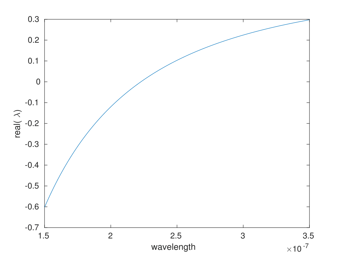
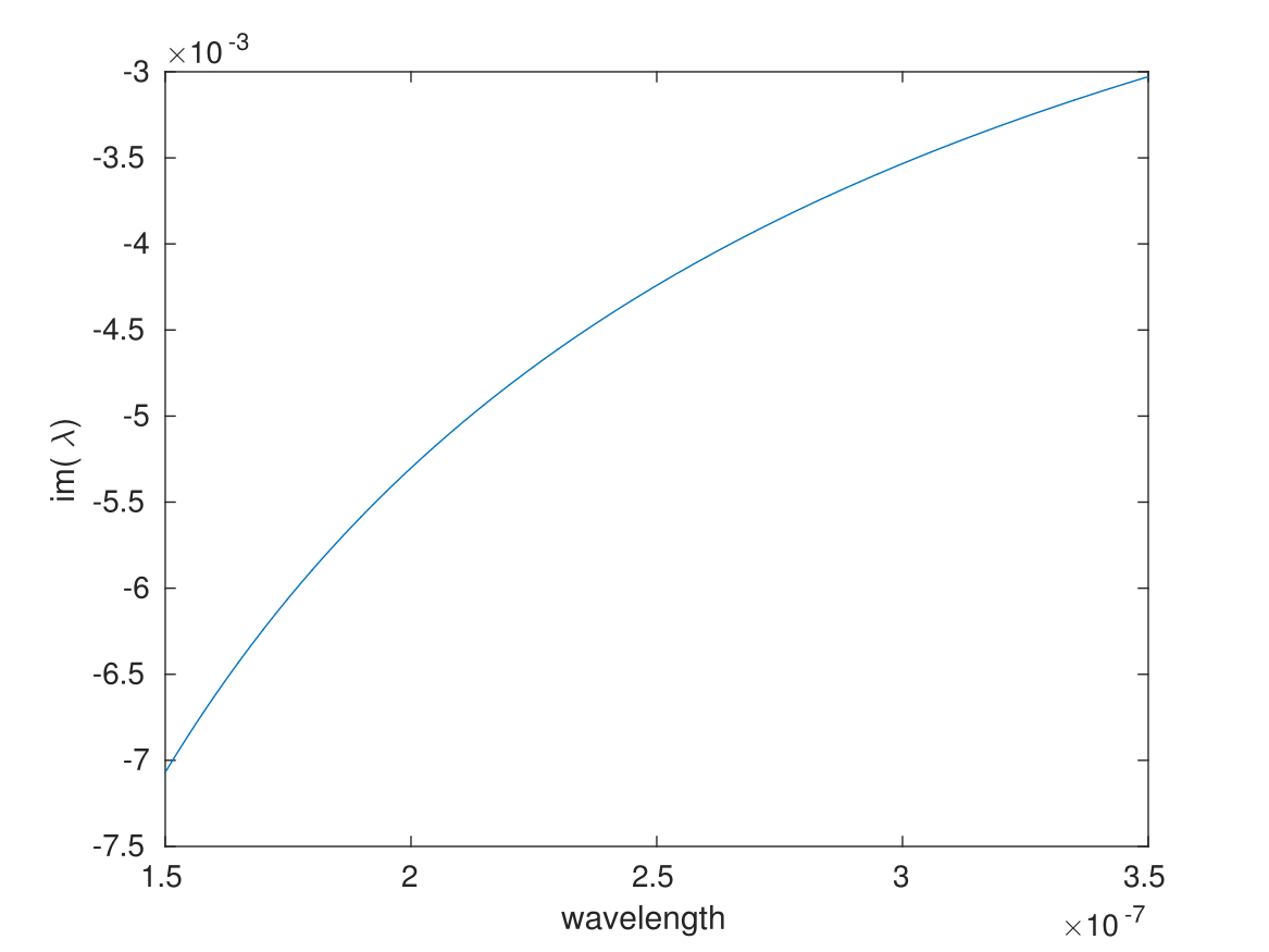
Figure 4.1 shows the variations of the real and imaginary parts of λ\lambda, defined by (2.3), as function of the wavelength using Drude’s model for σ=σ⁡(ω)\sigma=\sigma(\omega), which is depending on the operating frequency ω\omega [7].

Refer to caption
Refer to caption
Figure 4.1: Real and imaginary parts of λ\lambda as function of the wavelength.

As shown in Figure 4.1, the imaginary part of λ\lambda is very small. Therefore, when the real part of λ\lambda hits an eigenvalue that contributes to the first-order polarization tensor (and therefore to the plasmonic resonances), we should see a peak in the graph of |m11||m_{11}| and |M22c​c||M_{22}^{cc}| with respect to the wavelength. This allow us, in the case of class 𝒬\mathcal{Q} of algebraic domains, to recover λ+\lambda_{+} and λ+′\lambda_{+}^{\prime} and, in the case of two separated disks, to recover λϵ,1+\lambda_{\epsilon,1}^{+}.

Figures 4.2, 4.3, and 4.4 present examples of algebraic domains and their reconstructions, where a circle of radius one has been transformed for different values of mm and δ\delta.

Refer to caption
Refer to caption
Refer to caption
Refer to caption
Figure 4.2: From top to bottom and left to right: initial shape, reconstructed shape, |m11||m_{11}| and |M22c​c||M_{22}^{cc}| with respect to the wavelength for m=3m=3 and δ=0.066667\delta=0.066667.
Refer to caption
Refer to caption
Refer to caption
Refer to caption
Figure 4.3: From top to bottom and left to right: initial shape, reconstructed shape, |m11||m_{11}| and |M22c​c||M_{22}^{cc}| with respect to the wavelength for m=5m=5 and δ=0.03333\delta=0.03333.
Refer to caption
Refer to caption
Refer to caption
Refer to caption
Figure 4.4: From top to bottom and left to right: initial shape, reconstructed shape, |m11||m_{11}| and |M22c​c||M_{22}^{cc}| with respect to the wavelength for m=7m=7, δ=0.021978\delta=0.021978.

Figures 4.5 and 4.6 present examples of algebraic domains and their reconstructions, where a circle of radius one has been transformed for m=4m=4 and m=6m=6 and δ=0.02\delta=0.02.

Refer to caption
Refer to caption
Refer to caption
Refer to caption
Figure 4.5: From top to bottom and left to right: initial shape, reconstructed shape, |m11||m_{11}| and |M22c​c||M_{22}^{cc}| with respect to the wavelength for m=4m=4, δ=0.05\delta=0.05.
Refer to caption
Refer to caption
Refer to caption
Refer to caption
Figure 4.6: From top to bottom and left to right: initial shape, reconstructed shape, |m11||m_{11}| and |M22c​c||M_{22}^{cc}| with respect to the wavelength for m=6m=6, δ=0.02381\delta=0.02381.

Figures 4.7, 4.8, and 4.9 show examples of two circles of radius one separated by a distance ϵ\epsilon, and their reconstructions.

Refer to caption
Refer to caption
Refer to caption
Figure 4.7: From top left to bottom: initial shape, reconstructed shape and |m11||m_{11}| with respect to the wavelength for ϵ=2\epsilon=2.
Refer to caption
Refer to caption
Refer to caption
Figure 4.8: From top left to bottom: initial shape, reconstructed shape and |m11||m_{11}| with respect to the wavelength for ϵ=1.5\epsilon=1.5.
Refer to caption
Refer to caption
Refer to caption
Figure 4.9: From top left to bottom right: initial shape, reconstructed shape and |m11||m_{11}| with respect to the wavelength for ϵ=1.2\epsilon=1.2.

5 Concluding remarks

In this paper we have proved for a class of algebraic domains that the associated plasmonic resonances can be used to classify them. It would be very interesting to prove a similar result for all quadrature domains or all algebraic domains. We have also reconstructed the separation distance between two nanoparticles of circular shape from measurements of their first collective plasmonic resonances. Another challenging problem would be to generalize this result to more components and arbitrary shaped particles.

Appendix A Blow-up of the gradient of the potential at plasmonic resonances for two nearly touching disks

In this appendix, we consider two nearly touching disks and estimate the blow up of the gradient of the potential for two nearly touching disks at plasmonic resonances. We generalize to the plasmonic case, the estimates derived in [13, 11] for nearly touching disks with degenerate conductivities. In the nondegenerate case, we refer to [1, 12, 19, 26].

Let uu be the electric potential when an external potential HH is applied. In other words, uu satisfies

{Δ​u=0 in ​B1∪B2∪ℝ2∖(B1∪B2)¯,u|+=u|− on ​∂Bj,j=1,2,∂u∂ν|+=k​∂u∂ν|− on ​∂Bj,j=1,2,u⁡(𝐱)−H⁡(𝐱)=O⁡(|𝐱|−1) as ​|𝐱|→∞.\begin{cases}\displaystyle\Delta u=0\quad&\mbox{ in }B_{1}\cup B_{2}\cup\mathbb{R}^{2}\setminus\overline{(B_{1}\cup B_{2})},\\ \displaystyle u|_{+}=u|_{-}\quad&\mbox{ on }\partial B_{j},j=1,2,\\ \displaystyle\frac{\partial u}{\partial\nu}\Big|_{+}=k\frac{\partial u}{\partial\nu}\Big|_{-}\quad&\mbox{ on }\partial B_{j},j=1,2,\\ \displaystyle u(\mathbf{x})-H(\mathbf{x})=O(|\mathbf{x}|^{-1})\quad&\mbox{ as }|\mathbf{x}|\rightarrow\infty.\end{cases}

uu can be represented as follows:

u=H+𝕊⁡[φ],u=H+\mathbb{S}[\varphi],

where φ\varphi is the solution to

(λ​𝕀−𝕂∗)​[φ]=[∂νH|∂B1∂νH|∂B2].(\lambda\mathbb{I}-\mathbb{K}^{*})[\varphi]=\begin{bmatrix}\displaystyle\partial_{\nu}H|_{\partial B_{1}}\\ \displaystyle\partial_{\nu}H|_{\partial B_{2}}\end{bmatrix}.

Suppose that H⁡(x,y)=E0​xH(x,y)=E_{0}x. From (3.20), we obtain

(A.1) ∂H∂ν|ξ=±ξ0\displaystyle\frac{\partial H}{\partial\nu}|_{\xi=\pm\xi_{0}} =±E0h(ξ0,θ)α∑m=−∞∞(−|m|)e−|m|​ξ0+i​m​θ.\displaystyle=\pm E_{0}h(\xi_{0},\theta)\alpha\sum_{m=-\infty}^{\infty}(-|m|)e^{-|m|\xi_{0}+im\theta}.

On the other hand, by (3.17),

(A.2) [∂νH|∂B1∂νH|∂B2]=∑m=−∞∞E0​α​|m|​2​π​(1−e−2​|m|​ξ0)​e−|m|​ξ0​Ψϵ,m++0⋅Ψϵ,m−.\displaystyle\begin{bmatrix}\displaystyle\partial_{\nu}H|_{\partial B_{1}}\\ \displaystyle\partial_{\nu}H|_{\partial B_{2}}\end{bmatrix}=\sum_{m=-\infty}^{\infty}E_{0}\alpha|m|{\sqrt{2\pi(1-e^{-2|m|\xi_{0}})}}e^{-|m|\xi_{0}}\Psi^{+}_{\epsilon,m}+0\cdot\Psi_{\epsilon,m}^{-}.

Hence,

(A.3) φ=∑n≠01λ−λϵ,n+​(E0​α​|n|​2​π​(1−e−2​|m|​ξ0)​e−|m|​ξ0)​Ψϵ,n+.\displaystyle\varphi=\sum_{n\neq 0}\frac{1}{\lambda-\lambda_{\epsilon,n}^{+}}\Big(E_{0}\alpha|n|{\sqrt{2\pi(1-e^{-2|m|\xi_{0}})}}e^{-|m|\xi_{0}}\Big)\Psi_{\epsilon,n}^{+}.

Then (3.19) yields

(A.4) u=E0​x+E0​∑n≠0α​e−2​|n|​ξ0λ−λϵ,n+​sinh|n|ξ​ei​n​θ.\displaystyle u=E_{0}x+E_{0}\sum_{n\neq 0}\frac{\alpha e^{-2|n|\xi_{0}}}{\lambda-\lambda_{\epsilon,n}^{+}}\sinh|n|\xi\,e^{in\theta}.

Now we compute the electric field at the center of the gap ∇u​(ξ=0,θ=π)\nabla u(\xi=0,\theta=\pi). We have

∇u​(0,π)=E0​𝐞x+Ep​𝐞x,Ep=E0​∑n=1∞4​|n|​e−2​|n|​ξ0λ−λϵ,n+​(−1)n.\nabla u(0,\pi)=E_{0}\mathbf{e}_{x}+E_{p}\mathbf{e}_{x},\quad E_{p}=E_{0}\sum_{n=1}^{\infty}\frac{4|n|e^{-2|n|\xi_{0}}}{\lambda-\lambda_{\epsilon,n}^{+}}(-1)^{n}.

Let kϵ,n+=−coth⁡|n|​ξ0k_{\epsilon,n}^{+}=-\coth|n|\xi_{0}. Note that

λϵ,n+=kϵ,n++12​(kϵ,n+−1).\lambda_{\epsilon,n}^{+}=\frac{k_{\epsilon,n}^{+}+1}{2(k_{\epsilon,n}^{+}-1)}.

EpE_{p} can be rewritten as

Ep=E0​∑n=1∞(1−k)​(kϵ,n+−1)k−kϵ,n+​4​|n|​e−2​|n|​ξ0​(−1)n.E_{p}=E_{0}\sum_{n=1}^{\infty}\frac{(1-k)(k_{\epsilon,n}^{+}-1)}{k-k_{\epsilon,n}^{+}}4|n|e^{-2|n|\xi_{0}}(-1)^{n}.

Let us assume that kk is given by

k=kϵ,N++i​δ,k=k_{\epsilon,N}^{+}+i\delta,

for some N∈ℕN\in\mathbb{N}, where δ>0\delta>0 is a small parameter. This implies that, if δ\delta goes to zero, then the plasmon resonance occurs at the NN-th mode. For small δ>0\delta>0, EpE_{p} can be approximated by

(A.5) Ep≈E0​(1−k)​(kϵ,N+−1)k−kϵ,N+​4​N​e−2​N​ξ0​(−1)N.\displaystyle E_{p}\approx E_{0}\frac{(1-k)(k_{\epsilon,N}^{+}-1)}{k-k_{\epsilon,N}^{+}}4Ne^{-2N\xi_{0}}(-1)^{N}.

Since kϵ,N+≈−rN​ϵk_{\epsilon,N}^{+}\approx-\frac{\sqrt{r}}{N\sqrt{\epsilon}} for small ϵ>0\epsilon>0, we have

(A.6) Ep≈i​E0​rN​δ​ϵ​4​e−2​N​ξ0​(−1)N.\displaystyle E_{p}\approx iE_{0}\frac{r}{N\delta\epsilon}4e^{-2N\xi_{0}}(-1)^{N}.

It follows that

∇u​(0,π)≈i​E0​rN​δ​ϵ​4​e−2​N​ξ0​(−1)N​𝐞x.\nabla u(0,\pi)\approx iE_{0}\frac{r}{N\delta\epsilon}4e^{-2N\xi_{0}}(-1)^{N}\mathbf{e}_{x}.

References

  • [1] H. Ammari, E. Bonnetier, F. Triki, and M. Vogelius, Elliptic estimates in composite media with smooth inclusions: an integral equation approach, Annaes Sci. Ecole Normale Sup., 48 (2015), 453–495.
  • [2] H. Ammari, T. Boulier, J. Garnier, W. Jing, H. Kang, and H. Wang, Target identification using dictionary matching of generalized polarization tensors, Found. Comput. Math., 14 (2014), 27–62.
  • [3] H. Ammari, T. Boulier, J. Garnier, and H. Wang, Shape recognition and classification in electro-sensing, Proc. Natl. Acad. Sci. USA, 111 (2014), 11652–11657.
  • [4] H. Ammari, Y.T. Chow, K. Liu, and J. Zou, Optimal Shape Design by Partial Spectral Data, SIAM J. Sci. Comput., 37 (2015), B855-B883.
  • [5] H. Ammari, D. Chung, H. Kang, and H. Wang, Invariance properties of generalized polarization tensors and design of shape descriptors in three dimensions, Appl. Comput. Harmon. Anal., 38 (2015), 140–147.
  • [6] H. Ammari, G. Ciraolo, H. Kang, H. Lee, and G.W. Milton, Spectral analysis of a Neumann-Poincaré-type operator and analysis of cloaking due to anomalous localized resonance, Arch. Ration. Mech. Anal., 208 (2013), 667–692.
  • [7] H. Ammari, Y. Deng, and P. Millien, Surface plasmon resonance of nanoparticles and applications in imaging, Arch. Ration. Mech. Anal., 220 (2016), 109–153.
  • [8] H. Ammari, J. Garnier, W. Jing, H. Kang, M. Lim, K. Solna, and H. Wang, Mathematical and Statistical Methods for Multistatic Imaging, Lecture Notes in Mathematics, 2098. Springer, Cham, 2013.
  • [9] H. Ammari, J. Garnier, H. Kang, M. Lim, and S. Yu, Generalized polarization tensors for shape description, Numer. Math., 126 (2014), 199–224.
  • [10] H. Ammari and H. Kang, Polarization and Moment Tensors. With Applications to Inverse Problems and Effective Medium Theory, Applied Mathematical Sciences, 162. Springer, New York, 2007.
  • [11] H. Ammari, H. Kang, H. Lee, M. Lim, and H. Zribi, Decomposition theorems and fine estimates for electrical fields in the presence of closely located circular inclusions, J. Differ. Equat. 247 (2009), 2897–2912.
  • [12] H. Ammari, H. Kang, E. Kim, and M. Lim, Reconstruction of closely spaced small inclusions, SIAM J. Numer. Anal., 42 (2005), 2408–2428.
  • [13] H. Ammari, H. Kang, and M. Lim, Gradient estimates for solutions to the conductivity problem, Math. Ann., 332 (2), 277–286.
  • [14] H. Ammari, P. Millien, M. Ruiz, and H. Zhang, Mathematical analysis of plasmonic nanoparticles: the scalar case, arXiv:1506.00866.
  • [15] H. Ammari, M. Ruiz, S. Yu, and H. Zhang, Mathematical analysis of plasmonic resonances for nanoparticles: the full Maxwell equations, arXiv:1511.06817.
  • [16] K. Ando and H. Kang, Analysis of plasmon resonance on smooth domains using spectral properties of the Neumann-Poincaré operator, J. Math. Anal. Appl., 435 (2016), 162–178.
  • [17] K. Ando, H. Kang, and H. Liu, Plasmon resonance with finite frequencies: a validation of the quasi-static approximation for diametrically small inclusions, arXiv: 1506.03566.
  • [18] E. Bonnetier and F. Triki, On the spectrum of the Poincaré variational problem for two close-to-touching inclusions in 2D, Arch. Ration. Mech. Anal., 209 (2013), 541–567.
  • [19] E. Bonnetier and M. Vogelius, An elliptic regularity result for a composite medium with ”touching” fibers of circular cross-section, SIAM J. Math. Anal., 31 (2000), 651–677.
  • [20] M. Fatemi, A. Amini, and M. Vetterli, Sampling and reconstruction of shapes with algebraic boundaries, arXiv:1512.04388.
  • [21] D. Grieser, The plasmonic eigenvalue problem, Rev. Math. Phys. 26 (2014), 1450005.
  • [22] B. Gustafsson, C. He, P. Milanfar, and M. Putinar, Reconstructing planar domains from their moments, Inverse Problems, 16 (2000), 1053–1070.
  • [23] B. Gustafsson, M. Putinar, Topics on quadrature domains, Physica D 235(2007), 90-100
  • [24] J. Helsing and K.M. Perfekt, On the polarizability and capacitance of the cube, Appl. Comput. Harmon. Anal., 34 (2013), 445–468.
  • [25] J.B. Lasserre and M. Putinar, Algebraic-exponential data recovery from moments, Discrete Comput. Geom., 54 (2015), 993–1012.
  • [26] Y. Y. Li and M. Vogelius, Gradient estimates for solutions to divergence form elliptic equations with discontinuous coefficients, Arch. Ration. Mech. Anal., 153 (2000), 91–151.
  • [27] H. Kang, H. Lee, and M. Lim, Construction of conformal mappings by generalized polarization tensors, Math. Methods Appl. Sci. , 38 (2015), 1847–1854.
  • [28] D. Keren, D. Cooper, and J. Subrahmonia, Describing complicated objects by implicit polynomials, IEEE Trans. Pattern Anal. Mach. Intellig., 16 (1994), 38–52.
  • [29] R.C. McPhedran, L. Poladian, and G.W. Milton, Asymptotic studies of closely spaced, highly conducting cylinders, Proc. Royal Soc. A, 415 (1988), 185–196.
  • [30] K.M. Perfekt and M. Putinar, Spectral bounds for the Neumann-Poincaré operator on planar domains with corners, J. Anal. Math., 124 (2014), 39–57.
  • [31] Quadrature Domains and Their Applications, The Harold S. Shapiro Anniversary Volume (P.Ebenfelt, B.Gustafsson, D.Khavinson, M. Putinar, eds.) BirkhŠuser, Basel, 2005.
  • [32] G. Taubin, F. Cukierman, S. Sulliven, J. Ponce, and D.J. Kriegman, Parametrized families of polynomials for bounded algebraic curve and surface fitting, IEEE Trans. Pattern Anal. Mach. Intellig., 16 (1994), 287–303.