A Preliminary Jupiter ModelNote: Preprint: accepted 2/15/2016 for publication in Ap. J.
Abstract
In anticipation of new observational results for Jupiter’s axial moment of inertia and gravitational zonal harmonic coefficients from the forthcoming Juno orbiter, we present a number of preliminary Jupiter interior models. We combine results from ab initio computer simulations of hydrogen-helium mixtures, including immiscibility calculations, with a new nonperturbative calculation of Jupiter’s zonal harmonic coefficients, to derive a self-consistent model for the planet’s external gravity and moment of inertia. We assume helium rain modified the interior temperature and composition profiles. Our calculation predicts zonal harmonic values to which measurements can be compared. Although some models fit the observed (pre-Juno) second- and fourth-order zonal harmonics to within their error bars, our preferred reference model predicts a fourth-order zonal harmonic whose absolute value lies above the pre-Juno error bars. This model has a dense core of about 12 Earth masses, and a hydrogen-helium-rich envelope with approximately 3 times solar metallicity.
Keywords:
equation of state, hydrogen-helium mixtures, ab initio simulations, giant planets, extrasolar planetsI Introduction
In July 2016, the spacecraft will enter a bound orbit around Jupiter, and then complete further low-periapse orbits over a period of approximately one year. Measurements of the spacecraft’s accelerations may reach a precision of gal [11], allowing determination of Jupiter’s external gravitational potential, , to a relative precision approaching . In roughly the same time frame, the spacecraft will execute 22 low-periapse orbits around Saturn, making similar measurements of Saturn’s external gravity potential. The nonspherical components of provide information about a planet’s interior mass distribution.
In this paper, we construct static interior models intended to represent the present state of Jupiter, using a pressure-density relation derived from DFT-MD theory for the equation of state of the primary constituent of Jupiter and Saturn, a mixture of hydrogen and helium; see Militzer & Hubbard [18] and Militzer [17]. This barotrope is used to calculate the zonal harmonic coefficients , making various assumptions about the interior temperature distribution and core mass. Physically-motivated adjustments of the barotrope are made to achieve agreement with the observed (Table 1) and discrepancies with currently-observed higher are discussed. Lines 2-11 of Table 1 give calculated values from interior models discussed in Section 4.
To obtain a barotrope, we start with the grid of ab initio adiabats derived in Militzer [17] and Militzer & Hubbard [18]. These adiabats were determined with density functional molecular dynamics (DFT-MD) simulations using the Perdew-Burke-Ernzerhof (PBE) functional [24] in combination with a thermodynamic integration (TDI) technique to determine the full, nonideal entropy. The simulation cells contained a mixture of 18 helium and hydrogen atoms, corresponding to a helium mass fraction of =0.245, close to the solar value. As discussed in Militzer & Hubbard [18], each adiabat is characterized by the value of its absolute entropy per electron, , where is Boltzmann’s constant and is the number of electrons. Hereafter we denote this quantity with the simpler symbol .
Recently Becker et al. [1] constructed Jupiter models based on equations of state that were also derived with DFT-MD simulations but their approach differs in two respects. Becker et al. performed simulations for hydrogen and helium separately and then envoked the ideal mixing assumption while we simulated an interacting hydrogen-helium mixture directly. While we computed the full, nonideal entropy with TDI, Becker el at. obtained the entropy indirectly by fitting the internal energy and pressure, which are available in standard DFT-MD simulations. Becker et al. [1] reported deviations between 4 and 9% when they compared their EOS with Militzer & Hubbard [18]. Such deviations could have a significant repercussion on values of zonal harmonics for interior models.
In this paper, we use the term “entropy” and the symbol as a proxy for an adiabatic temperature vs. pressure relation for the fixed-composition mixture of H and He only (He mass fraction ), as determined by our detailed DFT-MD simulations. The simulations give the absolute entropy and other dependent variables as a function of and , for this specific composition. As discussed in Section III below, for the purpose of calculating general pressure-density relations, the same relation is taken to apply to adiabats with small, constant perturbations to the composition of the simulations. Moreover, the of the outermost layers of the model is determined by requiring a match to the Galileo Probe measurements of ; see Figure 5. The corresponding adiabat from our simulations has . Now, if we perturb this composition by changing and increasing , how might the adiabatic change, for bar, and how might this affect the barotrope? Let the Grüneisen parameter , where is the mass density. Suppose we have a compositional perturbation to and/or , of the order of . This might lead to a perturbation . Over a density range of three orders of magnitude, roughly spanning the jovian mantle, this value would imply a cumulative change of temperature of , with respect to the baseline . According Mie-Grüneisen theory [38], the thermal pressure makes up only 10% of the total pressure in the relevant Jupiter layers. Therefore, we expect the fractional change in density to be on the order of . This amount is so small that it is unlikely to affect any of our model predictions. It is certainly smaller than the previously-mentioned 4 to 9% discrepancy with Becker et al. [1].
Our ab initio calculations show that under jovian interior conditions, there is no distinct phase transition from molecular (diatomic, insulating) hydrogen to metallic (monatomic, conducting) hydrogen [31]. However, for convenience in this paper, the term “molecular” layer means layers at pressures below 1 Mbar, where the hydrogen is mostly diatomic. Likewise, the term “metallic” layer means layers at pressures above Mbar, but still external to a central dense core.
By combining our ab initio calculations for Jupiter’s interior adiabat [17] with the ab initio hydrogen-helium immiscibility calculations by Morales et al. [20], we predict that helium rain occurs in Jupiter’s interior. While the detailed physics and dynamics of helium rain is not yet understood, we make the assumption that this process introduces a superadiabatic temperature gradient and a compositional difference between the outer, molecular layer and inner, metallic layer. In our models, the of the molecular layer is set by the measurements of the Galileo entry probe while the of the metallic layer is a free parameter that we can adjust between two limits. The value of labeling for the metallic layer cannot be too high because otherwise no helium rain would have occurred in Jupiter according to DFT-MD simulations. The value of labeling cannot be below the Galileo value because, we assume, the cooling of the metallic layer is less efficient. The assumption of reduced cooling of the metallic layer is consistent with specific models constructed by Nettelmann et al. [23] who studied the evolution of jovian interior temperature profiles under the influence of H/He demixing and layered double diffusive convection (see upper left-hand panel of Figure 10 of that paper).
For the molecular layer, we assume the helium abundance that was measured by the Galileo probe [30, 16]. We derive the helium contents in the metallic layer by assuming the planet as a whole has a protosolar helium abundance [15]. The distribution of heavier elements throughout the planet is not well understood. The capture of comets has enriched the envelope over time. Similarly the erosion of the core may have added icy and rocky materials to the envelope [35, 36, 32, 5]. Given these uncertainties, we introduce three model parameters: the mass of today’s dense core, the heavy element (“metals”) mass fraction in the molecular layer and that in the metallic layer. We assume that both layers are homogeneous and interpolate between both compositions to derive an estimate for the structure of the helium rain layer. Model predictions are not sensitive to details of this procedure because, in Jupiter, the interpolation layer between 1 and 2 Mbar contains very little mass.
This article is organized as follows. In Section 2, we describe how we deal with hydrogen-helium immiscibility. In Section 3, we discuss how one perturbs the helium abundance in a particular EOS and how heavy elements are introduced. In Section 4, we discuss the EOS of different planetary ices and present results from additional ab initio simulations. In Section 5, we introduce our reference Jupiter model and discuss variations from it. Before we conclude, we describe in Section 6 how the moment of inertia is derived from CMS theory. In the Appendix, we provide additional details about the CMS calculations.
II Adiabats and Hydrogen-Helium Immiscibility


Figure 1 shows a plot of temperature, , versus pressure, , for a family of such adiabats as well as the hydrogen-helium immiscibility domain derived from ab initio simulations by Morales et al. [20]. These simulations also used the DFT-MD technique in combination with the PBE functional and TDI method to compute the entropy. They are thus fully compatible with the abiabats from Militzer & Hubbard [18]. As is evident in Figure 1, the interiors of both Jupiter and Saturn enter a region at a pressure 1 Mbar where helium in solar proportion to hydrogen becomes immiscible. Both planets are thus are likely to have layers with helium rain. Figure 2 depicts the location of this layer in Jupiter. This prediction is a direct consequence of combining the ab initio immiscibility and adiabat calculations with measurements of the planets’ tropospheric vs. profiles [27, 14]. No temperature or pressure adjustments of the immiscibility domain were needed.
Heavy elements were not considered in this analysis. Depending on the concentration, a small correction to the adiabatic profile would be plausible. We also note that Morales et al. [20] performed the immiscibility calculations for which differs slightly from the protosolar value. However, this concentration difference does not change the immiscibility temperature to a significant degree. Based on the analysis in Nettelmann et al. [23], we estimate this correction to be of the order 160 K only.
The hydrogen-helium immiscibility hypothesis was first invoked to explain Saturn’s luminosity excess [28, 29]. In the immiscibility layer, helium droplets would form and rain down into the deeper interior, resulting in a gradual removal of helium from the planets outer layer. The associate release of gravitational energy provides an energy source to explain Saturn’s luminosity excess.
Whether helium rain occurs on Jupiter is less certain. Its interior is hotter and no helium rain is need to explain its present luminosity [4]. The Galileo entry probe measured a small helium depletion in Jupiter’s upper atmosphere (0.234 by mass compared to 0.274, the protosolar value [15]. Perhaps the strongest evidence for helium rain to occur on this planet comes from the depletion of neon. The Galileo measurements showed that there is ten times less neon in Jupiter’s atmosphere compared to solar values. Wilson & Militzer [34] demonstrated with ab initio simulations that neon has a strong preference for dissolving in the forming helium droplets. This offered an explanation for the neon depletion and provided strong, though indirect evidence for helium rain to occur on Jupiter.
According to the more recent ab initio calculations, the present Jupiter would encounter the immiscibility domain at pressures above Mbar (Figure 1). In Saturn, the domain is entered at Mbar. If a cooling scenario for Jupiter or Saturn involves a steady decrease of entropy with time, then the onset of helium rain would occur when the interior adiabat first touches the boundary of the helium immiscibility domain. The curvature of the boundary is such that a H-He adiabat with 7.20 osculates the boundary at Mbar and K.
We are thus faced with the task of deriving a barotrope for present-day Jupiter which is consistent with the properties of dense, hot hydrogen-helium mixtures shown in Figure 1 and with Jupiter’s presumed cooling history. A detailed, dynamical calculation of the process of helium rain and subsequent evolution of Jupiter’s interior temperature profile is beyond the scope of the present paper, whose aim is to infer a jovian barotrope based on current knowledge of Jupiter’s composition and thermal state, and on current results from ab initio simulations of hydrogen-helium mixtures at high pressure. The resulting barotrope is used here to predict Jupiter’s higher zonal harmonic coefficients, whose values are to be measured by Juno.
Thus, we make the simplifying assumption that the cooling of early Jupiter to an interior adiabat 7.20, corresponding the onset of immiscibility, then leads to reduced heat transport in the region around Mbar, effectively slowing interior temperature decline, while layers at lower pressures continue to transfer heat to Jupiter’s atmosphere. In this scenario, the present-day Jupiter barotrope for pressures Mbar lies on the Galileo Probe adiabat with reduced He abundance, but at somewhat higher pressures, temperatures follow a higher-entropy adiabat with a slightly-above protosolar helium abundance, . The interior adiabat would be expected to lie between 7.20 (for no heat transport across the immiscibility region) and 7.08 (for efficient heat transport across the immiscibility region). In the study that we present here, our preferred model has an interior adiabat with 7.13 (shown as a heavy line in Figure 3). We refer to this model as Model DFT-MD 7.13; Its parameters are shown in boldface in Table 1. The barotrope for Model DFT-MD 7.13 shown in Figure 4. The corresponding profile is shown in Figure 5.


III Compositional Perturbations to Equation of State
In order to derive general barotropes, we must now evaluate the effects of (1) varying He concentration, and (2) varying metallicity. The barotrope shown in Figures 4 and 5 corresponds to an initial He mass fraction and metals mass fraction . Since this composition is a good initial approximation to the Jupiter envelope, we use a perturbation approach to derive the effects of compositional changes. Let the reference barotrope for and be . Although this barotrope is computed with detailed DFT-MD simulations not assuming an ideal mixture of H and He, to simplify this derivation we approximate it by an additive volume law, , valid for a noninteracting mixture:
| (1) |
where 0.755. We now want to change the abundance of helium to and metals to . We assume that the temperature-pressure relation is unchanged under perturbations to the composition (i.e., the perturbing admixture is chemically and thermodynamically inert). With this assumption and the additive volumes approximation, , the perturbed density is given by,
| (2) |
where and is the volume and density of the metals component. Rewriting Equations (1) and (2), we find
| (3) |
with all densities evaluated for the reference . The same equation is obtained if one starts from a fully interacting hydrogen-helium equation of state and then perturbs the helium and metals abundances.
For the composition in Jupiter’s outer layers, at Mbar, we adopt abundances from Galileo Probe measurements [37]. In this region the main contributors to are the molecules and , and for the abundance we adopt the largest value measured by the probe (rather than assuming a solar abundance for H2O). Neglecting other metals, we obtain 0.7498, 0.2333, 0.0169, for the presumed jovian composition at layers with 1 Mbar.
Using a DFT-MD equation of state for pure He (Militzer 2008) along the shown in Figure 5, we obtain the density-pressure relation shown in Figure 6.
IV Equation of State of H2O, CH4, and NH3
Evaluation of the perturbation term in Eq.(3) is somewhat more complex because of the presence of multiple molecular species, but need not be highly precise because the contribution of this term is comparatively small. We continue to assume, for pressures above and below the He-immiscibility gap, that the main contributors to the mass fraction are the molecules , , and , in solar proportions. Thus, to evaluate , it is necessary to evaluate the density change of these molecular entities along the jovian . We thus performed a number of DFT-MD simulations of , , and under such conditions.
All simulations were performed with the VASP code [13] using the PBE functional. Pseudopotentials of the projector-augmented wave type [2] and a plane wave basis set cutoff of 1100 eV were employed. The zone-average point, , was used to sample the Brillouin zone. A time step of 0.2 fs was used. Density, temperature, and composition were prescribed in the simulations. After an initial equilibration period, the pressure was derived by averaging over the MD simulation.
We first benchmarked our simulations by comparing our results with the shock wave measurements by Nellis et al. [21] that compressed a mixture of water, ammonia, and isopropanol (C3H8O) to 200 GPa. This mixture, labeled “synthetic Uranus”, was designed to resemble the different planetary ices in the outer solar system. The concentrations of the heavy nuclei (C:O=0.529, N:O=0.162) indeed closely resemble solar proportions. However, the mixtures is somewhat depleted in hydrogen (H:O=3.54) while one would expect a H:O ratio of 4.60 if one mixes H2O, CH4, and NH3 in O:C:N proportions that were used in the experiments. This difference prompted us to perform two sets of simulations. First we studied a hydrogen-depleted mixture, H:O:C:N=87:25:13:4, that closely resembles the “synthetic Uranus” mixture within the size constraints of typical simulations that accomodate between 100 and 200 atoms.
Our simulation results in Table 2 show excellent agreement with the experimental findings. It should be noted that if we prescribe the central values for densities and temperature, that were measured in the experiments, then our computed pressures were, respectively, slightly higher and slightly lower than those reported in the experiments. However, if we adjusted the density and temperatures in our simulations within the experimental 1 uncertainties then our computed pressures fall within the experimental error bars of the two available measurements. This provides another example for DFT-MD simulations that closely reproduce experimental findings [12].
In Table 2, we also report results from simulations of a H:O:C:N=99:21:12:3 mixtures that exactly represent the hydrogen contents of a solar H2O, CH4, and NH3 mixture. Because of the higher hydrogen content, the density is lower than that of “synthetic Uranus” when compared for the same and . The simulation results were incorporated into Figures 7 and 8.
Figure 7 shows calculations used to perform the estimation of . In the low-pressure region of this figure, pressure-density values for , , and are combined assuming ideal mixing. In the lower left-hand part of this figure, orange dots show the ideal-gas partial pressure of an ideal mixture of the three molecules along the jovian , with virial corrections up to Kbar. Dash-dot curves at the top of the figure show zero-temperature relations calculated from quantum-statistical models and tabulated in Zharkov & Trubitsyn [38]. The orange dashed curve shows the resulting zero-temperature relation for a solar mixture of the three molecules. Dots in the upper right-hand corner of this figure show finite-temperature calculations for pressures greater than a megabar; Figure 8 shows a zoom of this region, along with experimental data points for “synthetic Uranus” [21].
To construct in the gap between low pressure and high pressure, we perform a linear interpolation in log-log space as indicated in Figure 7.
Figure 9 shows (dashed curve) for assumed Galileo Probe composition (for pressures below 2 Mbar). As a hypothesis to be tested by our preliminary Jupiter model, we assume that all jovian layers at pressures less than Mbar have the composition measured by the Galileo Probe, with a corresponding correction to the density given by Equation (3). In this pressure range, we find from Figure 6 and Figure 9 that 0.48 and 0.38, leading to 0.995. The latter number is fortuitously close to unity because the slightly lower Galileo Probe He abundance (relative to the DFT-MD simulations) is almost compensated by the presence of metals.
Note that is depleted relative to and in the Galileo Probe data. That is, Galileo Probe data show approaching a solar ratio to hydrogen-helium, while and are approximately three times their solar ratio to hydrogen-helium.
In contrast, for solar proportions of :: and for 1 Mbar, we have 0.38, and 0.42 through the bulk of the jovian envelope (Figure 9, solid curve).
For layers at pressures greater than 2.7 Mbar, we take the He and metals abundances to be slightly higher than the protosolar values 0.2741 and 0.0149 [15]. Our DFT-MD equation of state, combined with the constraints of Jupiter’s total mass, volume, and and any reasonable interior temperature distribution, does not imply a large increase of above its protosolar value, for otherwise the densities would be too large. Assuming 0.0246 in the deeper layers and taking into account a slight He enrichment caused by depletion in Jupiter’s outer layers, we get 0.2788. The assumed value of corresponds to abundances of and , relative to H, that are 4 times protosolar. Because of the much larger protosolar value of relative to H, a similar 4 times enhancement of this molecule leads to larger and hence interior densities, and the resulting models would be outside the acceptable range. We get 0.0246 if we take the enhancement of to be 2.4 times protosolar.
We insert this value in Equation (3) for the presumed jovian composition at layers with 2 Mbar. Then, over a pressure range corresponding to the bulk of the jovian envelope, Mbar, we find from Figure 6 and Figure 9 that 0.49 and 0.42, leading to 0.959.
As is obvious from these results, and has long been known, the presence of metals in Jupiter only affects the barotrope at the level of a few percent. Thus modeling the abundance and distribution of metals in Jupiter by matching the planet’s gravity data necessarily requires very accurate (better than 1%) knowledge of .
V Jupiter Models
V.1 Spheroid Parameters and Code Function
The version of the concentric maclaurin spheroid (CMS) code that we use is designed to automatically calculate a mass distribution with a total mass equal to Jupiter’s mass, g, and an equatorial radius km. The latter is the observed equatorial radius of a layer at an average pressure of 1 bar, and the tabulated are normalized to this radius. We assume that Jupiter rotates as a solid body with period [26] . CMS theory is constructed to find a rotationally-distorted model for the dimensionless small parameter
| (4) |
which to lowest order in is equivalent to , see Equation (A2), but is more convenient as it can be directly computed from observed quantities.
Models are calculated with spheroids. Using the notation of Hubbard [9], the dimensionless equatorial radii of the spheroids are specified as follows. By definition 1 for the outermost spheroid (its equatorial radius ). The innermost spheroid surface is placed at (i.e., the core’s equatorial radius ). The choice of core radius is somewhat arbitrary: the external zonal harmonic coefficients are sensitive to the total core mass but insensitive to its density. Models have 170 spheroids equally spaced in in the range and another 339 spheroids in the range . (where in this region the spacing , or 105.6 km). The outermost spheroid () has zero density and is spaced (or 53 km) above the next spheroid ().
We verified that zonal gravitational harmonic results were unaffected by the details of the spheroid spacing, by carrying out subsidiary calculations with spheroids equally spaced from core to surface. As shown in Figure 13 for a typical Jupiter interior model, spheroids interior to make no significant contribution to the . Therefore we chose a closer spacing of spheroids exterior to , to improve accuracy.
As outlined in Hubbard [9], two nested iterations are required to obtained a converged rotationally-distorted model fitted to a given barotrope . Before the iterations begin, a provisional density distribution is specified, with each spheroid having a constant density . For the specified , the shape and total potential of each spheroid is then iteratively calculated until relative changes between iterations fall below a specified tolerance, usually . Typically, this requires iterations. After satisfactory convergence, the total mass of the configuration is obtained by summing over all spheroids.
An outer iteration loop (typically iterations) is performed to converge the model to the specified barotrope . As described by Hubbard [9], using the and equipotential shapes from the converged inner loop, the average pressure between the upper and lower surface of each spheroid is calculated. Then using the , the barotrope relation is solved for each spheroid to obtain new density values, . The core spheroid is not included in this procedure as it is assumed to be an incompressible high-density region. See Section 17 for details on the convergence of the iterations.
Define the renormalization constant . After the latest outer iteration, we renormalize all the by multiplying each value (including the core) by the factor . These new are then passed to the inner iteration loop, where the spheroid shapes and corresponding external are computed, and then (which depends on the spheroid shapes) is computed. The resulting configuration is then passed back to the outer loop.
The final result of the two iteration loops is a model with converged , a mass and rescaled density of the incompressible core, and spheroids fitted to the scaled prescribed barotrope . The model conforms precisely to the prescribed values of , , and . The scaled barotrope corresponding to this model is convenient for comparing with barotropes for various values of and , e.g. of the form of Equation (3), in which the initial DFT-MD simulations for are rescaled by a (roughly constant) factor to account for new values of and . Values of for each model are used to obtain results for the model’s metals content , as entered in Table 1.
Introduction of the renormalization constant provides a convenient method for efficiently exploring the parameter space of jovian models, because, as discussed in Section IV, to first approximation the density of a perturbed mixture of H, He, and metals is related to the reference mixture by the divisor which is nearly constant over a broad range of pressures. Thus if , the overall metals content of the model is reduced with respect to the assumed starting barotrope, and vice versa.
V.2 Parameters of Barotrope and Core
For the reader’s assistance, Table 3 briefly defines a number of relevant parameters.
As discussed by Militzer et al. [19], it is difficult to fit the pre-Juno values of Jupiter’s , especially , with a constant-entropy, constant-composition barotrope and uniform rotation. Although the H-He DFT-MD equation of state has been updated since 2008, see Militzer & Hubbard [18] and Militzer [17], the difficulty remains. For comparison purposes, we include at the end of Table 1 two interior models (denoted as SC) that we computed using the same CMS procedure as the other models, but with the older equation of state of Saumon et al. [25]. These SC models are able to match the pre-Juno and with vanishingly-small cores and tens of Earth masses of metals in the envelope (see Table 1). Why are our DFT-MD models so different? Although central temperatures for DFT-MD and SC models are similar (see Table 1), it turns out that mid-envelope temperatures for adiabatic DFT-MD models are considerably cooler. This behavior is a consequence of the depression of the adiabatic temperature gradient associated with hydrogen metallization, as discussed by Militzer & Hubbard [18] and Militzer [17]. Such behavior is not exhibited by the SC EOS and may not be incorporated in the other recent Jupiter models. Cooler temperatures, as well as revisions to the pressure-density relation, result in somewhat higher mass densities in the middle envelope, with respect to the other models. It is this effect, in our models, that is primarily responsible for considerably reduced envelope metallicity, larger core mass, and increased .
In 2008 we attempted to reduce the absolute value of by hypothesizing a subrotating layer below Jupiter’s observable atmosphere, but this assumption is not supported by any realistic circulation model. It is possible to obtain a model which fits the pre-Juno value of by instead introducing a chemical change and corresponding extra density increase at layers around Mbar, but such models are not grounded in any fundamental calculations of the thermodynamics of dense hydrogen plus impurities, and are inconsistent with reasonable barotropes. In this paper we take a different approach. We use the Morales et al. [20] prediction for the pressure-temperature conditions of H/He immiscibility. Then we assume helium rain also introduces a composition change. As discussed in Section 3, for Mbar, we have 0.995, while for Mbar, if one has four times solar (primordial) abundances of , , and times , and no other metals, as the composition at depth, one would have 0.959. These numbers suggest an expected extra density change resulting from the presence of a phase-separation region and an increase of metallicity and helium to approximately proto-solar values at deeper layers. As we discuss in more detail below, we need a much larger extra density change () to obtain a DFT-MD model with reduced enough to agree with the pre-Juno value.
To treat the expected extra density change, in the pressure range between 1 and 2 Mbar we interpolate linearly in and between the low-pressure barotrope with and the high-pressure barotrope with , noting that at 2.7 Mbar lies on a higher-entropy adiabat than the atmospheric adiabat. Results for gravitational harmonic coefficients of models are insensitive to the thickness of this narrow interpolation region. A CMS boundary could of course be placed at a discrete location to exactly treat an actual density discontinuity, but the resulting change to the gravitational harmonic coefficients would be negligible.
The models presented in this paper are intended to correspond closely to the theoretical behavior of hydrogen-helium mixtures and to properties of the outer jovian layers as constrained by the Galileo Probe.
The CMS method generates models that exactly fit the total jovian mass and 1-bar equatorial radius. We adjust the density (and thus the mass) of the schematic central core of all models to obtain a match to the pre-Juno observed value of given in Table 1, in the expectation that a more precise post-Juno value will not differ significantly from this number. The other parameter beside the core mass that is poorly constrained is the entropy of the deep adiabat, which we vary from the Galileo Probe value 7.08 through the value that osculates the immiscibility boundary, 7.20, on up to (as an extreme case) 7.24. With increasing , the thermal contribution to the deep pressure increases, yielding lower density for a given pressure, thus accommodating a slight increase in metallicity . As we see from Table 1, the predicted higher-order gravitational harmonic coefficients vary from one model to the next at the level of for (readily measurable by Juno), to for , to for . The values appear to have less value for discriminating interior structure, but their near-constancy at a total level of may be useful as a reference for discerning the signature of nonhydrostatic effects at a similar level, such as deep interior dynamics [11].
By increasing the density by an additional amount in the vicinity of the He-immiscibility zone, it is possible to obtain a match to Jupiter’s pre-Juno and with a suitable model. But, as noted by Militzer et al. [19], one does not have free rein in this process because Jupiter’s barotrope must correspond to a physically-plausible composition. Because the DFT-MD barotrope is generally denser than the corresponding barotrope that one would compute using the theory of Saumon et al. [25], in our DFT-MD models very little enhancement of metals can be tolerated in Jupiter’s envelope.
Most of our models are calculated using (for Mbar) the barotrope , corresponding to the Galileo Probe and abundances, and the barotrope for Mbar, corresponding to an adiabat with entropy , (enhanced) protosolar helium abundance , and , corresponding to Galileo-Probe enhancement of methane and ammonia and a lesser enhancement of water, but no presence of denser species such as magnesium-silicates. During the CMS calculations we linearly interpolate in vs. across the immiscibility region between 1 and 2.7 Mbar. All models in Table 1 labeled DFT-MD (with no parenthesis) have the indicated compositions in the molecular and metallic regions respectively. As the deep increases, such models show a modest increase in metallicity in the hydrogen-helium envelope exterior to the dense core, as characterized by the parameter , the total mass of metals in Earth masses.
Model DFT-MD 7.13 has , meaning that the input barotrope yields a match to the total planetary mass without rescaling the densities. A characteristic of DFT-MD 7.13 warrants discussion. This model has Galileo Probe abundances of CH4, NH3, and H2O throughout the molecular layer, and solar abundances of CH4, and NH3 in the metallic layer. The metallic layer has solar H2O, more than in the molecular layer; a full solar H2O enhancement would yield total densities which are too large to fit the total mass of Jupiter. As discussed in Section IV, the assumed composition and temperature profile results in a reasonable relation, which results in a reasonable planetary model. However, acceptable relations only limit the possible range of temperature profiles and metallicities but do not uniquely constrain them.
As alternatives, we investigated two variants of our preferred model, in which we imposed equal metallicities in the molecular and metallic layers. Model DFT-MD 7.13 (low-) has artificially low in both layers (although He abundance does increase from the Galileo probe value to the protosolar value). This unrealistic model has the largest and core mass of the suite. At the opposite extreme, Model 7.24 (equal-) has the same metallicity in both layers, and also has a relatively large .
All models shown in Table 1 have core mass adjusted to give agreement to seven significant figures with the observed value . Two of the models, DFT-MD 7.15(J4) and SC 7.15(J4), include an additional density (and metallicity) increase across the immiscibility region between 1 and 2 Mbar, adjusted to yield agreement with the pre-Juno observed values of and . We note that uncertainties in observed values in Table 1 are formal error bars; none of our models would be ruled out by these pre-Juno measurements if the true error bars are times larger. All of our models are close to the pre-Juno observed value of , but the agreement may be fortuitous.
V.3 Comparison of Barotropes with Models
Figure 10 shows a plot of polar and equatorial density profiles for our preferred model DFT-MD 7.13.
Figure 11 plots the density vs. pressure profile for preferred model DFT-MD 7.13 (grey stairstep), along with the input barotrope. Figure 12 is a close-up of the high-pressure region of Figure 11. The weighting functions for contributions to the external zonal harmonic coefficients, for the preferred model, are shown in Figure 13.

Model DFT-MD 7.15(J4) reduces to the observed value by decreasing the barotrope’s density at low pressures, and increasing the density at high pressures. However, densities in the outer region at pressures below 1 Mbar then correspond to unphysical negative metallicity. The entry for this model in Table 1 shows a total metals content exterior to the dense core; this value is the sum of in the H-He envelope at pressures greater than Mbar, and (unphysical) at lower pressures. We are unable to find a consistent DFT-MD Jupiter model that matches the observed and values in Table 1.
VI Moment of Inertia
Jupiter’s normalized moment of inertia NMoI (where is the moment of inertia about the rotation axis) is in principle separately measurable from the , and is a separate constraint on interior structure. Helled et al. [8] investigate models with fixed values of and and conclude that a range of NMoI values between 0.2629 and 0.2645 can be found. Nettelmann et al. [22] calculate a moment of inertia but normalize it to the mean radius of the 1-bar equipotential surface, a model-dependent quantity with a precision limited to third order in their perturbative theory of figures. However, their result is in reasonable agreement with values that we calculate below. Since the nonperturbative approach of our present investigation virtually eliminates any uncertainty in the theoretical calculation of the , here we explore the subject further as a guide to measurement requirements for the Juno spacecraft.
Once a converged interior model is obtained, the NMoI is given exactly by the expression
| (5) |
in the notation of Hubbard [9].
Although Equation (5) resembles the Radau-Darwin relation in that it seemingly relates the NMoI to , it actually has no relationship because Equation (5) shows that for a fixed , an infinity of different CMS density distributions could enter into the first term. On the other hand, since each of those CMS density distributions is required to yield the fixed , the range of variation of NMoI is in actuality quite restricted. To illustrate the point, in Figure 14 we show the cumulative value of the NMoI as a function of the CMS radius , for preferred model DFT-MD 7.13. The cumulative value of is obtained by partially summing the expression in Equation (5) from the central CMS () out to a CMS with dimensionless equatorial radius .
To illustrate how details of interior structure affect the total NMoI, Figure 15 shows the difference of the cumulative values of , for the preferred model minus model SC 7.15.

To truly discriminate between models with different barotropes, it will be necessary to measure the NMoI to about five significant figures, posing a difficult challenge to Juno or other future investigations. Figure 16 illustrates the point.

We should point out that a measurement of Jupiter’s NMoI would actually be obtained from a measurement of the planet’s spin angular momentum, . Thus if Jupiter were to rotate differentially on cylinders with significant mass involved in the various rotation zones, the tightly constrained values of NMoI that we find here might be broadened to some extent. It remains to be determined whether measurement of NMoI will prove to be more of a constraint on the possibility of deep differential rotation, or on the range of possible interior barotropes.
VII Discussion and Conclusions
The combination of the DFT-MD equation of state and observed already strongly limit the parameter space of acceptable pre-Juno models.
Our study has the following new features: (a) We eliminate arbitrary density enhancements to fit the gravity field; instead we utilize the H-He immiscibility phase boundary computed by Morales et al. [20] to bound the location and magnitude of a helium-related compositional change; (b) Our models incorporate the latest version of the DFT-MD equation of state, replacing the widely-used SC EOS theory [25]; (c) We utilize CMS theory for the first time to calculate high-order zonal harmonic coefficients for realistic Jupiter models.
It is important to note that for fixed , the computed value of is sensitive to the density in the region of Jupiter’s metallic-hydrogen envelope where He immiscibility is predicted. One may force an agreement with the pre-Juno value of given in Table 1 by imposing a density enhancement across the interpolation region which is much larger than the implied by an increase in He to the primordial value above 2.7 Mbar. However, when this is done, conservation of mass leads to a model with (formally) negative metallicity in the low-pressure outer envelope.
The new DFT-MD equation of state generally yields a very limited suite of interior models of relatively low metallicity. These models could be falsified by forthcoming Juno gravity data.
In Jupiter model DFT-MD 7.13, about 0.83 of the total mass is between the He-immiscibility region near 1 Mbar pressure and the core-mantle boundary. So if in this region, the mass of metals outside the core would comprise , to be added to a core mass , for a total Jupiter metallicity . As shown in Table 1, most of the other DFT-MD models have similar total metallicities. In contrast, our models based on the SC EOS (last two lines in Table 1) have total metallicities that are about 60% higher, in qualitative agreement with earlier results obtained by Guillot et al. [7] and Guillot [6] that were also derived using the SC equation of state. The latter studies included the possibility that Jupiter’s core mass might be zero, and our independent SC models also show very small core masses.
The inferred large core masses of our DFT-MD models are consistent with a core-nucleated scenario for the formation of Jupiter [3]. The overall metallicity of Jupiter implied by most of our models is roughly three times protosolar, implying that about two-thirds of the volatile protosolar nebular complement to the refractory core was not incorporated in primordial Jupiter.
In summary, we are able to derive Jupiter interior models that match measured values of , and sometimes , and , and are consistent with predictions from published ab initio simulations of hydrogen and helium, and additional results for different planetary ices, H2O, CH4, and NH3 that we report here. In our preferred model, the heavy element abundance in the metallic layer is equivalent to a three-fold solar concentration of all three ices. The preferred value for the concentration in the molecular layer is slightly less but consistent with the Galileo measurements.
Our preferred model has a massive core of 12 Earth masses which is very similar to our earlier model [19]. When one uses the semi-analytical equation of state (SC EOS) of Saumon et al. [25] instead of our ab initio DFT-MD EOS, a much smaller core of 4 Earth masses is predicted for the same model assumptions. This illustrates how sensitively some model predictions depend on the details of hydrogen-helium EOS.
Our Jupiter model is preliminary and intended for use as a reference for comparison with experimental results from the Juno orbiter and other data sources. New data will tell us how well the model works.
Appendix A Definitions for theory of figures
The external potential of a liquid planet in hydrostatic equilibrium rotating at a uniform rate is usually expanded on Legendre polynomials as
| (A1) |
where is the gravitational constant, the planet’s mass, km is the normalizing radius, is the cosine of the angle from the rotation axis, and the radial distance from the center of mass. Pre- values of Jupiter’s zonal harmonic coefficients are given in the first line of Table 1, and are identical to values cited by Militzer et al. [19].
It is expected that the gravity experiment will improve the precision of the harmonic coefficients by at least two orders of magnitude and measure the coefficients to degree 10 and possibly beyond. Values of the provide integral constraints on the mass distribution within Jupiter, and can thus be used to constrain interior models. As discussed by Hubbard et al. [10], the basic parameter that determines the magnitude of the is the dimensionless number (to lowest order, is the ratio of the magnitude of the rotational acceleration to gravitational acceleration, at the planet’s equator),
| (A2) |
where is Jupiter’s mean density. Zharkov & Trubitsyn [38] show that one may write
| (A3) |
where the dimensionless response coefficients, , can be obtained from the solution of a hierarchy of nonlinear perturbation equations. These response coefficients in turn depend on the equation of state relating the pressure to the mass density at each point within the planet. Provided that a barotropic relation exists and that the planet is in hydrostatic equilibrium, the perturbative potential-theory approach of Zharkov & Trubitsyn [38] can be used. However, for Jupiter and for Saturn, and the dimensionless coefficients do not decline rapidly with and . Replacing the infinite sum in Equation (A3) with a finite sum up to, say might suffice to determine the measurable to better than Juno precision, but would entail evaluation of lengthy analytic expressions. Instead, in this paper we use the more straightforward non-perturbative concentric maclaurin spheroid (CMS) theory of figures of Hubbard [9].
Appendix B Numerical precision of CMS calculations
Figure 17 shows the improvement in the values for a typical model over 50 steps in the outer iteration loop. After 50 iterations, the change in and higher degrees has fallen below the computer’s floating point precision. The change in after 50 steps is at the level of , much smaller than the precision with which it can be measured.

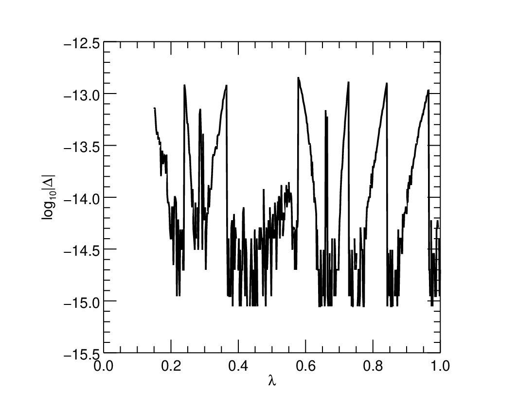
Figure 18 shows the relative error in the CMS calculation of the gravitational potential on the level surfaces of a converged model using the audit-point method described in Hubbard et al. [10].
References
- [1] Becker, A., Lorenzen, W., Fortney, J., Nettelmann, N., Schöttler, M., & Redmer, R. 2014, Astrophys. J. Supp., 215, 21
- [2] Blöchl, P. E. 1994, Phys. Rev. B, 50, 17953
- [3] D’Angelo, G., Weidenschilling, S. J., Lissauer, J. J., & Bodenheimer, P. 2014, Icarus, 241, 298
- [4] Fortney, J. J., & Hubbard, W. B. 2004, Astrophys. J., 608, 1039
- [5] Gonzalez-Cataldo, F., Wilson, H. F., & Militzer, B. 2014, Astrophys. J., 787, 79
- [6] Guillot, T. 1999, Planetary and Space Science, 47, 1183
- [7] Guillot, T., Gautier, D., & Hubbard, W. B. 1997, Icarus, 130, 534
- [8] Helled, R., Anderson, J., Schubert, G., & Stevenson, D. 2011, Icarus, 216, 440
- [9] Hubbard, W. B. 2013, Astrophys. J., 768, 43
- [10] Hubbard, W. B., Schubert, G., Kong, D., & Zhang, K. 2013, Icarus, 242, 138
- [11] Kaspi, Y., Hubbard, W. B., Showman, A. P., & Flierl, G. R. 2010, Geophys. Res. Lett., 37, L01204
- [12] Knudson, M. D., Desjarlais, M. P., Lemke, R. W., Mattsson, T. R., French, M., Nettelmann, N., & Redmer, R. 2012, Phys. Rev. Lett., 108, 091102
- [13] Kresse, G., & Furthmüller, J. 1996, Phys. Rev. B, 54, 11169
- [14] Lindal, G. F., Sweetnam, D. N., & Eshleman, V. R. 1985, Astron. J., 90, 1136
- [15] Lodders, K. 2003, Astrophys. J., 591, 1220
- [16] Mahaffy, P. R., Niemann, H. B., Alpert, A., Atreya, S. K., Demick, J., Donahue, T. M., Harpold, D. N., & Owen, T. C. 2000, J. Geophys. Res., 105, 15061
- [17] Militzer, B. 2013, Phys. Rev. B, 87, 014202
- [18] Militzer, B., & Hubbard, W. B. 2013, Astrophys. J., 774, 148
- [19] Militzer, B., Hubbard, W. H., Vorberger, J., Tamblyn, I., & Bonev, S. A. 2008, Astrophys. J. Lett., 688, L45
- [20] Morales, M. A., Hamel, S., Caspersen, K., & Schwegler, D. M. E. 2013, Phys. Rev. B, 87, 174105
- [21] Nellis, W., Holmes, N., Mitchell, A., Hamilton, D., & Nicol, M. 1997, J. Chem. Phys., 107, 9096
- [22] Nettelmann, N., Becker, A., Holst, B., & Redmer, R. 2012, Astrophys. J., 750, 52
- [23] Nettelmann, N., Fortney, J., Moore, K., & Mankovich, C. 2015, MNRAS, 447, 3422
- [24] Perdew, J. P., Burke, K., & Ernzerhof, M. 1996, Phys. Rev. Lett., 77, 3865
- [25] Saumon, D., Chabrier, G., & Horn, H. M. V. 1995, Astrophys. J. Suppl., 99, 713
- [26] Seidelmann, P. K., et al. 2007, Celestial Mechanics and Dynamical Astronomy, 98, 155
- [27] Seiff, A., et al. 1998, J. Geophys. Res., 103, 22857
- [28] Stevenson, D., & Salpeter, E. 1977a, Astrophys. J. Suppl. Ser., 35, 221
- [29] —. 1977b, Astrophys. J. Suppl., 35, 239
- [30] von Zahn, U., Hunten, D. M., & Lehmacher, G. 1998, J. Geophys. Res., 103, 22815
- [31] Vorberger, J., Tamblyn, I., Militzer, B., & Bonev, S. 2007, Phys. Rev. B, 75, 024206
- [32] Wahl, S. M., Wilson, H. F., & Militzer, B. 2013, Astrophys. J., 773, 95
- [33] Weast, R. C. 1972, Handbook of Chemistry and Physics 53rd Ed. (Chemical Rubber Co.), D–166
- [34] Wilson, H. F., & Militzer, B. 2010, Phys. Rev. Lett., 104, 121101
- [35] —. 2012a, Astrophys. J, 745, 54
- [36] —. 2012b, Phys. Rev. Lett., 108, 111101
- [37] Wong, M., Mahaffy, P. R., Atreya, S. K., Niemann, H. B., & Owen, T. C. 2004, Icarus, 171, 153
- [38] Zharkov, V. N., & Trubitsyn, V. P. 1978, Physics of Planetary Interiors (Pachart, Tucson)
| (all ) | ||||||||||
|---|---|---|---|---|---|---|---|---|---|---|
| (K) | ||||||||||
| pre-Juno observed | ||||||||||
| (JUP230)aaObserved values are from R. A. Jacobson (2003), JUP230 orbit solution, with . All theoretical models match to seven significant figures. | ||||||||||
| DFT-MD 7.24 | 0.212 | 0.26387 | 12.5 | 0.9 | 10.3 | 0.07 | 17600 | |||
| DFT-MD 7.24 (equal-) | 0.26385 | 13.1 | 1.1 | 7.5 | 0.07 | 17650 | ||||
| DFT-MD 7.20 | 0.211 | 0.26388 | 12.3 | 0.8 | 9.9 | 0.07 | 17260 | |||
| DFT-MD 7.15 | 0.211 | 0.26389 | 12.2 | 0.7 | 9.2 | 0.07 | 16860 | |||
| DFT-MD 7.15 () | 0.26399 | 14.9 | 0.08 | 16770 | ||||||
| DFT-MD 7.13 | 0.26389 | |||||||||
| DFT-MD 7.13 (low-) | 0.26381 | 14.0 | 0.2 | 1.1 | 0.05 | 16820 | ||||
| DFT-MD 7.08 | 0.26390 | 0.6 | 8.3 | 0.07 | 16220 | |||||
| SC 7.15 | 0.26392 | 3.5 | 28.2 | 0.11 | 18020 | |||||
| SC 7.15 () | 0.26394 | 3.2 | 29.3 | 0.12 | 17310 |
| Method | H:O | C:O | N:O | (g cm-3) | (K) | (GPa) |
|---|---|---|---|---|---|---|
| Experiment | 3.54 | 0.529 | 0.162 | 2.044 0.005 | 3220 200 | 49.9 0.5 |
| Simulation(a) | 3.48 | 0.520 | 0.160 | 2.044 | 3220 | 52.17 0.17 |
| Simulation(a) | 3.48 | 0.520 | 0.160 | 2.039 | 3020 | 50.17 0.30 |
| Experiment | 3.54 | 0.529 | 0.162 | 2.45 0.13 | 4100 300 | 110 4 |
| Simulation(a) | 3.48 | 0.520 | 0.160 | 2.450 | 4100 | 96.34 0.42 |
| Simulation(a) | 3.48 | 0.520 | 0.160 | 2.580 | 4400 | 114.47 0.35 |
| Simulation(b) | 4.71 | 0.571 | 0.143 | 2.353 | 4100 | 117.90 0.32 |
| Simulation(b) | 4.71 | 0.571 | 0.143 | 2.262 | 4100 | 105.37 0.25 |
| Simulation(b) | 4.71 | 0.571 | 0.143 | 3.011 | 7000 | 264.92 0.48 |
| Simulation(b) | 4.71 | 0.571 | 0.143 | 3.592 | 8000 | 431.78 0.34 |
| Simulation(b) | 4.71 | 0.571 | 0.143 | 3.940 | 9000 | 559.32 0.42 |
| Simulation(b) | 4.71 | 0.571 | 0.143 | 4.550 | 10000 | 811.62 0.56 |
| Parameter(s) | Definition |
|---|---|
| , | mass fractions of H and He in DFT-MD simulations; see Equation (1) |
| mass density of H-He mixture in DFT-MD simulations, for given and | |
| , , | perturbed mass fractions of H, He, and metals; see Equation (2) |
| total mass fraction of “metals” in Jupiter (including dense core) | |
| ratio of mass density for reference barotrope, Equation (1), to | |
| mass density with perturbed , , | |
| ratio of mass density for reference barotrope, Equation (1), to | |
| mass density of pure He at same and | |
| ratio of mass density for reference barotrope, Equation (1), to | |
| mass density of a pure “metals” mixture at same and | |
| mass of the Earth | |
| total mass of in Jupiter’s molecular layer; see Table 1 | |
| total mass of in Jupiter’s metallic layer; see Table 1 | |
| temperature at the core-mantle boundary, generally at 40 Mbar; | |
| see Table 1 | |
| dimensionless factor applied to prescribed barotrope to yield | |
| exact Jupiter mass; equivalent to compositional perturbation |