Adjoint master equation for Quantum Brownian Motion

Technical improvements in quantum experiments are making impressive steps forward, reaching levels of accuracy which were hardly imaginable a few decades ago. Controlling the noise is often the crucial challenge for further progress, and a theoretical understanding is important to disentangle environmental effects from intrinsic properties of the system.

Quantum Brownian motion [1, 2, 3, 4, 5, 6] is the paradigm of an open quantum system interacting with an external bath, and nowadays it finds applications in several physical contexts such as chemistry [7], condensed matter [8, 9, 10], bio-physics [11, 12, 13, 14] and opto-mechanics [15, 16, 17, 18] to name a few.

The model consists of a particle $S$ of mass $M$, with position $\hat{x}$ and momentum $\hat{p}$, harmonically trapped at frequency $\omega_{\text{\tiny S}}$ and interacting with a thermal bath of independent harmonic oscillators, with positions $\hat{R}_{k}$, momenta $\hat{P}_{k}$, mass $m$ and frequencies $\omega_{k}$. This model has become a milestone in the theory of open quantum system [19, 20, 21, 22, 23, 24, 25, 26, 27, 28, 29, 30, 31, 32, 33, 2, 34]. The total Hamiltonian $\hat{H}_{\text{\tiny T}}$ of system plus bath is $\hat{H}_{\text{\tiny T}}=\hat{H}_{\text{\tiny S}}+\hat{H}_{\text{\tiny I}}+\hat{H}_{\text{\tiny B}},$ where

are respectively the system, bath and interaction Hamiltonians. The characterization of the set of coupling constants $C_{k}$ is provided by the spectral density which is defined as

The first master equation for this model was derived by Caldeira and Leggett [26] by using the common assumption of a factorized initial state

where $\hat{\rho}_{\text{\tiny S}}(0)$ and $\hat{\rho}_{\text{\tiny B}}$ are the initial states of the system and of the bath respectively, and also the Born-Markov approximation [2]; The high temperature limit was taken into account in order to obtain a simple evolution [35, 36, 37] in the Lindblad form with constant coefficients:

where $\gamma$ and $\beta$ are the damping rate and the inverse temperature, respectively. This derivation has two limitations. First, the master equation is the generator of a dynamical map which is not positive [38, 39], i.e. it does not map all quantum states $\hat{\rho}_{\text{\tiny S}}$ into quantum states ¹¹ 1 Although the Caldeira-Leggett master equation (4) is not completely positive, it becomes of use when large time scales are considered. In fact, after a transient time of the order of $\sim\gamma^{-1}$, the dynamical map corresponding to Eq. (4) maps quantum states in quantum states. This is however still not sufficient to obtain in general the same asymptotic expectation values one obtains from the exact model. In order to avoid subsequent gross miscalculations, one needs to implement some effective modifications on the initial conditions [60, 61, 30].. Second, the regime of validity cannot be always fulfilled: the latest attempts to reach the ground state at low temperature regimes [18, 40] is an opto-mechanical example.

The main contributions in overcoming these limitations were given by Haake and Reibold [30] and later by Hu, Paz and Zhang [33], who provided the exact master equation for the particle $S$ given the total Hamiltonian $\hat{H}_{\text{\tiny T}}$:

where $\hat{H}(t)$ and the coefficients $\gamma(t)$, $h(t)$ and $f(t)$ now are time dependent. We refer to this model as to the Quantum Brownian Motion (QBM) model. Contrary to the Caldeira-Leggett master equation, which is valid only for the specific ohmic choice the spectral density ($J(\omega)\propto\omega$) Eq. (5) is valid for arbitrary spectral densities $J(\omega)$ and temperatures $T$. However, for the QBM model, the coefficients are solutions of differential equations, which in general are hard to solve. The explicit form of these coefficients, beyond the weak-coupling limit [33], was provided by Ford and O’Connell in [41].

The generality of such a solution is outstanding, however, as noticed in [41], solving the time-dependent master equation is in general a formidable problem. The authors show that the dynamics of the system can be more easily solved by working with the Wigner function of the system and bath at time $t$ and then averaging over the degrees of freedom of the bath. According to their procedure, the reduced Wigner function $W$ at time $t$ can be expressed in terms of that at time $t=0$ as follows:

where $P$ describes the transition probability [41].

The drawback of such a procedure is the limited selection of initial states $\hat{\rho}_{\text{\tiny S}}$ for which the Wigner function is analytically computable. For gaussian states this is not a problem, however there exist physical relevant situations where this is not the case [42, 43, 44]. An example is provided by a system initially confined in a infinite square potential. We will refer explicitly to this example.

In this paper, we propose an alternative derivation of the QBM dynamics for a general bath at arbitrary temperatures. The master equation we derive is exact and of course is equivalent to Eq. (5). However, the time-dependent coefficients will be written in a much simpler form, and therefore can be used to compute much more easily the solution of the master equation, regardless of the strength of the coupling and of the form of the initial state $\hat{\rho}_{\text{\tiny S}}$.

The paper is organized as follows: In section II we describe our alternative derivation. In section III we derive the master equation. In section IV we provide a criterion for the complete positivity of the dynamics. In section V we derive the explicit evolution of some physical quantities one is typically interested in, for a specific spectral density, in particular we compare our result with that of Haake-Reibold [30] and Hu-Paz-Zhang [33]. Moreover, we will show how one can easily go beyond the results of Ford and O’Connell [41] and compute the time evolution of expectations values for initial non-gaussian states.

We derive the adjoint master equation for the quantum Brownian motion model. This is the dynamical equation describing the time evolution of a generic operator $\hat{O}$ of the system $S$, once the average over the bath is taken. To this end, we consider the unitary time evolution of the extended operator $\hat{O}\otimes\bf{\hat{1}_{B}}$ with respect to the total Hamiltonian $\hat{H}_{\text{\tiny T}}$ of the system plus bath, where $\bf{\hat{1}_{B}}$ is the bath identity operator, and we trace over the degrees of freedom of the bath. The time derivative of the reduced operator, under the hypothesis of a factorized initial state as in Eq. (3), will be governed by the adjoint master equation.

Let us consider the von Neumann representation [45, 46] of the operator $\hat{O}$, defined, at time $t=0$, by the following relation:

where $\mathcal{O}(\lambda,\mu)$ is the kernel of the operator $\hat{O}$ and $\hat{\chi}(\lambda,\mu,t=0)=\exp[i\lambda\hat{x}+i\mu\hat{p}]$ is the generator of the Weyl algebra, also called characteristic or Heisenberg-Weyl operator [46]. Following the procedure previously outlined, and using the von Neumann representation, the operator $\hat{O}$ at time $t$ is given by:

where we introduced the characteristic operator at time $t$:

and $\hat{\mathcal{U}}_{t}=\exp(-\tfrac{i}{\hbar}\hat{H}_{\text{\tiny T}}t)$. Therefore, to obtain the evolution of the operator $\hat{O}_{t}$, it is sufficient to consider the evolution equation for the characteristic operator:

where $\hat{x}(t)$ and $\hat{p}(t)$ are the position and momentum operators of the system $S$ evolved by the unitary evolution generated by the total Hamiltonian of the composite system plus bath and $\hat{\rho}_{\text{\tiny B}}$ is defined in Eq. (3).

In order to obtain the explicit expression of $\hat{x}(t)$ and $\hat{p}(t)$, we rewrite the bath and interaction Hamiltonian defined in Eq. (1) in terms of the creation and annihilation operators $\hat{b}^{\dagger}_{k}$ and $\hat{b}_{k}$ of the $k$-th bath oscillator: $\hat{H}_{\text{\tiny B}}=\sum_{k}\hbar\omega_{k}\hat{b}_{k}^{\dagger}\hat{b}_{k}$ and $\hat{H}_{\text{\tiny I}}=-\hat{x}\hat{B}(0)$, where $\hat{B}(t)$ is defined as

In terms of the latter we solve the Heisenberg equations of motions for $\hat{x}(t)$ and $\hat{p}(t)$ by using the Laplace transform. The solutions are:

where $\hat{x}$ and $\hat{p}$ denote the operators at time $t=0$, and the two Green functions $G_{1}(t)$ and $G_{2}(t)$ are defined as

where $\mathcal{L}$ denotes the Laplace transform and $\omega_{\text{\tiny R}}^{2}=\omega_{\text{\tiny S}}^{2}+\tfrac{2}{M}\int d\omega\,J(\omega)/\omega$. In Eq. (13) we introduced the dissipation kernel $D(t)$:

Given Eqs. (12), since the operators of the system and of the bath commute at the initial time, it follows that:

where $\alpha_{1}(t)$ and $\alpha_{2}(t)$ are defined as follows:

and the operator $\hat{\chi}_{\text{\tiny B}}(t)$ refers only to the degrees of freedom of the bath:

Under the assumption of a thermal state for the bath:

the trace over $\hat{\chi}_{\beta}(t)$ gives a real and positive function of time $\text{Tr}^{(\text{\tiny B})}\left[\hat{\rho}_{\text{\tiny B}}\hat{\chi}_{\text{\tiny B}}(t)\right]=e^{\phi(t)}$, where the explicit form of $\phi(t)$ can be obtained by using the definition of the spectral density in Eq. (2). In Appendix A we present the explicit form of $\phi(t)$, written as the sum of three terms: $\phi(t)=\lambda^{2}\phi_{1}(t)+\mu^{2}\phi_{2}(t)+\lambda\mu\phi_{3}(t)$. The time derivative of $\hat{\chi}_{t}$ gives

by substituting this expression in:

we arrive at the adjoint master equation for the operator $\hat{O}_{t}$.

The integral in Eq. (20) depends on the choice of the kernel $\mathcal{O}(\lambda,\mu)$. On the other hand, we want an equation that can be directly applied to a generic operator $\hat{O}$ without having first to determine its kernel. This means that we want to rewrite Eq. (19) in the following time-dependent form

where the effective Hamiltonian $\hat{H}_{\text{\tiny eff}}(t)$, the hermitian Kossakowski matrix $\bm{K}(t)$ and the Lindblad operators $\hat{L}_{a}$ should not depend on the parameters $\lambda$ and $\mu$. Then, the linearity of Eq. (20) will allow to extend Eq. (21) to any operator $\hat{O}_{t}$. To achieve this, the explicit dependence from the parameters $\lambda$ and $\mu$, contained in the coefficients $\alpha_{i}$ and $\phi(t)$, must disappear in Eq. (19). This can be done in the following way. Let us consider the commutation relations among $\hat{x}$, $\hat{p}$ and $\hat{\chi}_{t}$:

Given Eqs. (16), we can express $\lambda\hat{\chi}_{t}$ and $\mu\hat{\chi}_{t}$ as a linear combination of the above commutators. Then, by using this result, we can easily rewrite Eq. (19) in the form given by Eq. (21), where

the Lindblad operators are $\hat{L}_{1}=\hat{x}$ and $\hat{L}_{2}=\hat{p}$. The time dependent function $\Gamma^{\text{\tiny A}}(t)$, $\Delta^{\text{\tiny A}}(t)$ and the elements of the Kossakowski matrix $K_{a,b}(t)$ are reported in Appendix B. An important note: one of the elements of the Kossakowski matrix vanishes $K_{22}(t)=0$. This means that the term corresponding to $[\hat{p},[\hat{p},\hat{\rho}_{\text{\tiny S}}]]$ is absent, as for the Caldeira-Leggett master equation [26]. In the latter case this implies the non complete positivity of the dynamics. In the case under study, complete positivity is instead automatically satisfied, as it is explicitly shown in Sec. IV. This result is in agreement with previous results [30, 33, 41, 47].

Eq. (21) is linear in $\hat{\chi}_{t}$ and does not depend on $\lambda$ and $\mu$. Therefore because of Eq. (20), it holds for any operator $\hat{O}_{t}$: $\tfrac{d}{dt}\hat{O}_{t}=\mathbb{L}_{t}[\hat{O}_{t}]$, as in Eq. (21). This is the adjoint master equation and $\mathbb{L}_{t}$ is the generator of the dynamics. The correspondent adjoint dynamical map is given by

The result here obtained is very general and depends only on the form of the total Hamiltonian $\hat{H}_{\text{\tiny T}}$ defining the QBM model together with the separability of the initial total state (Eq. (3)), but does not depend on the particular initial state of the system $S$. We now show that we recover the master equation (5) for the states.

We now derive the master equation for the density matrix, starting from the adjoint master equation. For a time independent adjoint master equation, switching to the master equation for the states is straightforward: the adjoint dynamical map ${\bm{\Phi}_{t}}$ is $\exp\left(t\mathbb{L}\right)$, where the generator $\mathbb{L}$ is time independent. Therefore the map ${\bm{\Phi}_{t}}$ and its generator $\mathbb{L}$ commute. Then the generator of the dynamics for the states is equal to the adjoint of the generator of the dynamics for the operators. In the time dependent case here considered, instead, the procedure is more delicate. Consider the dynamical map ${\bm{\Phi}_{t}^{*}}$ for the states:

which is the adjoint map of ${\bm{\Phi}_{t}}$ defined in Eq. (24). The adjointness, denoted here by the $*$-symbol, has to be understood in the following sense:

where $\braket{\ \cdot\ }=\text{Tr}^{(\text{\tiny S})}\left[\ \cdot\ \hat{\rho}_{\text{\tiny S}}(0)\right]$. Let us consider the time derivative of $\braket{\hat{\chi}_{t}}$ and let us express it as follows:

The above equation defines the two maps ${\bm{\Lambda}_{t}}$ and ${\bm{\Lambda}_{t}^{*}}$. According to Eq. (21),

On the other hand, according to standard practice [2], the map ${\bm{\Lambda}_{t}^{*}}$ in Eq. (27) is defined as

where the map $\tilde{\mathbb{L}}^{*}_{t}$ is the generator of the dynamics for the states. By adjointness we have

Then, by comparison we have to construct the map $\tilde{\mathbb{L}}_{t}$ as follows:

In terms of this latter expression, Eq. (28) becomes

For a time dependent generator, in order to construct the master equation for the states we need to derive explicitly the form of $\tilde{\mathbb{L}}_{t}$. This is derived in Appendix C and the final result is:

where $\hat{L}_{\alpha}$ is defined after Eq. (23),

and the elements of $\tilde{K}_{ab}(t)$ are reported in the Appendix. Now, in order to obtain the time derivative of the operator $\hat{O}_{t}$ at time $t$, we act with $\tilde{\mathbb{L}}_{t}$ on the operator $\hat{O}(0)$ at time $t=0$ and then with the adjoint dynamical map ${\bm{\Phi}_{t}}$, as described in Eq. (32). The latter equation, according to the definition of the map ${\bm{\Lambda}_{t}}$ in Eq. (28), gives $\tfrac{d}{dt}\hat{O}_{t}$. From this we can compute the master equation for the states. This can be simply done by using the cyclic property of the trace $\text{Tr}^{(\text{\tiny S})}\left[\ \cdot\ \right]$ applied on the expression in Eq. (33). Then, we have:

which yields the master equation for the states of the system $S$:

This is the desired result, which naturally coincides with the QBM master equation (5). The explicit form of the terms in Eq. (36) can be obtained starting from the spectral density $J(\omega)$ defined in Eq. (2).

We now discuss the complete positivity of the dynamical map ${\bm{\Phi}_{t}}$ generated by the generator $\mathbb{L}_{t}$ defined in Eq. (21). The action of this dynamical map on the generic operator $\hat{O}$ of the system $S$ is

which is the combination of two completely positive maps: the unitary evolution provided by the total Hamiltonian of system plus bath, and the trace over the bath. Therefore, by construction the dynamical map is completely positive. However, two observations are relevant here. First, it is instructive to verify explicitly the complete positivity of the dynamics. Second, in a situation where approximations are needed in order to compute explicitly the coefficients of the (adjoint) master equation, the verification of the complete positivity of the dynamics becomes a fundamental point of interest.

When the generator $\mathbb{L}$ of the dynamics is not time dependent, the sufficient and necessary condition for the complete positivity of the dynamical map is the positivity of the Kossakowski matrix [36, 48]. For a time dependent generator $\mathbb{L}_{t}$, instead, a positive Kossakowski matrix is only a sufficient condition for complete positivity. An example is precisely the QBM model under study, whose Kossakowski matrix is not positive for all times, nevertheless the dynamics is completely positive. For a time dependent generator, a necessary and sufficient condition instead is given by the following theorem [49, 50], under the assumption of a Gaussian channel.

Suppose that the action of a gaussian dynamical map ${\bm{\Phi}_{t}}$ on the characteristic operator $\hat{\chi}$ of the system is defined as follows

where ${\bm{X}}_{t}$ and ${\bm{Y}}_{t}$ are $2\times 2$ matrices describing the evolution of the characteristic operator

and $\bra{\xi}=(\lambda,\mu)$ and $\bra{R}=(\hat{x},\hat{p})$. In terms of ${\bm{X}}_{t}$, ${\bm{Y}}_{t}$ and of the symplectic matrix ${\bm{\Omega}}=\bigl(\begin{smallmatrix}0&&1\\ \ -1&&0\end{smallmatrix}\bigr)$, we can define the following matrix ${\bm{\Psi}}_{t}$:

The necessary and sufficient condition for the dynamical map ${\bm{\Phi}_{t}}$ to be completely positive (CP) is the positivity of ${\bm{\Psi}}_{t}$ for all positive times. Since the matrix ${\bm{\Psi}}_{t}$ is a $2\times 2$ matrix, the request of its positivity reduces to the request of positivity of its trace and determinant:

The condition of positivity of the trace, Eq. (41a), is easily verified for all physical spectral densities: the spectral density is positive by definition, see Eq. (2), and this implies the negativity of $\phi_{1}(t)$ and $\phi_{2}(t)$, see Eqs. (54), for all positive values of the temperature. On the other hand, the second condition, Eq. (41b), cannot be easily verified in general. Once a specific spectral density $J(\omega)$ is chosen, one can check explicitly whether $\text{det}\left[{\bm{\Psi}}_{t}\right]\geq 0$. For example, the spectral density $J(\omega)\propto\omega$, originally chosen in [26] to describe the quantum brownian motion, does not satisfy the above condition also in the case of no external potentials, and in fact it is well known that the Caldeira-Leggett master equation is not CP.

As already remarked, the QBM model automatically guarantees complete positivity. However, in practical cases one is not able to compute explicitly the time dependent coefficients of the Kossakowski matrix. Approximations are needed, in which case complete positivity is not automatically guaranteed anymore. This can be checked in a relatively easy way by assessing the positivity of $\text{det}\left[{\bm{\Psi}}_{t}\right]$.

The original QBM master equation (5) is expressed in terms of functions (forming the Kossakowski matrix), whose explicit expression is not easy to derive, even if one considers the solution given in [41]. They are solutions of complicated differential equations, difficult to solve except for very simple situations. More important, expectation values are not easy to compute: one has to determine the state of the system at time $t$, which is in general a formidable problem also in a particularly simple situation. In our derivation, instead, the use of the adjoint master equation provides an much easier tool for the computation of expectation values. The evolution is expressed in the Heisenberg picture, therefore it does not depend on the state of the system $S$ but only on the properties of the adjoint evolution ${\bm{\Phi}_{t}}$.

For example, by plugging the expression of $\hat{x}^{2}(t)$ (obtained from Eq. (12)) in Eq. (21) we obtain an equation for the expectation value $\braket{\hat{x}^{2}_{t}}$:

which can be solved directly without having to solve a more complicated system of differential equations, as it is necessary when the solution is in the Schrödinder picture [2], as well as for the case of the Wigner function approach [51, 52, 41]. Once the interaction with the bath, i.e. the spectral density function, is specified, $G_{1}(t)$ and $G_{2}(t)$ can be determined as described before, and this fully determines the time evolution of $\braket{\hat{x}^{2}_{t}}$ in terms of the initial expectation values. In a similar way one can compute all the other expectation values as a function of time.

To show this, we provide the explicit general solution of some physical quantities of interest for a specific spectral density. We consider: the diffusion function $\Lambda^{\text{\tiny dif}}(t)=\braket{\hat{x}^{2}_{t}}-\braket{\hat{x}_{t}}^{2}$, the energy of the system $E(t)=\braket{\hat{p}^{2}_{t}}/2M+\tfrac{1}{2}M\omega_{\text{\tiny S}}^{2}\braket{\hat{x}_{t}^{2}}$ and the decoherence function $\Gamma_{dec}(t)$. The latter is defined as follows. We consider a particle which, at time $t=0$, is described by a state $\Ket{\psi(t=0)}=\mathcal{N}[\Ket{\alpha}+\Ket{\beta}]$, where $\Ket{\alpha}$ and $\Ket{\beta}$ are two equally spread out, with spread equal to $\sigma_{0}$, gaussian wave packets, centered respectively in $x_{\alpha}=\braket{\alpha|\hat{x}|\alpha}$ and $x_{\beta}=\braket{\beta|\hat{x}|\beta}$ and $\mathcal{N}$ is the normalization constant. The probability density in position $x$ at time $t$ is [2]:

where $\rho_{\alpha\beta}(x,t)=\braket{x|\text{Tr}^{(\text{\tiny B})}\left[\mathcal{U}_{t}(\Ket{\alpha}\Bra{\beta})\mathcal{U}_{t}^{{\dagger}}\right]|x}$: there is a modulation given by the phase $\varphi(x,t)$ and a reduction of the interference contrast determined by the decoherence function $\Gamma^{\text{\tiny dec}}(t)<0$. The decoherence function takes the following form:

where $\Delta_{x}$ and $\Delta_{p}$ are the distances between the two guassians in position and momentum, and the function $\phi_{1}(t)$ is defined in Eq. (54a). The explicit expressions for $\Lambda^{\text{\tiny dif}}(t)$ and $E(t)$ is given in Appendix D.

As a concrete example, we consider the case of the Drude-Lorentz spectral density

which is commonly used for example in light-harvesting systems [53, 13], where $\Omega$ is the characteristic frequency of the bath. The corresponding dissipation and noise kernels, defined in Eq. (14) and Eq. (55) respectively, are:

where the function $\Phi_{L}$ is the Hurwitz-Lerch transcendent function $\Phi_{L}(z,s,a)=\sum_{n=0}^{+\infty}z^{n}(n+a)^{-s}$. The two Green functions are:

and $G_{1}(t)=\tfrac{d}{dt}G_{2}(t)$, where $C_{1}$, $C_{2}$ and $C_{3}$ are the complex roots of the polynomial $y(s)=(y^{2}+\omega_{\text{\tiny S}}^{2}+2\gamma\Omega)(y+\Omega)-2\gamma\Omega^{2}$ and $D_{i}=\prod_{j=1,j\neq i}^{3}(C_{i}-C_{j})$. In terms of these functions, we can compute the functions $\phi_{i}(t)$ with the help of Eqs. (54) as well as the three relevant quantities previously discussed, whose explicit expressions are displayed in Eq. (44), Eq. (72) and Eq. (73).

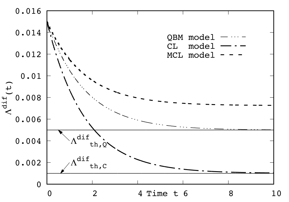
Fig. 1 and 2 show the evolution of the diffusion function $\Lambda^{\text{\tiny dif}}(t)$, of the energy $E(t)$ and of the decoherence function $\Gamma^{\text{\tiny dec}}(t)$, and we compare their time evolution according to the QBM model as described here above (QBM), with that of the Caldeira-Leggett (CL) master equation in (4). We also consider the evolution given by the Modification of the Caldeira-Leggett (MCL) master equation, which is obtained from Eq. (4) by adding the term $-\tfrac{\gamma\beta}{8M}[\hat{p},[\hat{p},\hat{\rho}_{\text{\tiny S}}(t)]]$ to guarantee the complete positivity of the dynamics [38, 39, 2]. As for the initial state, in Fig. 1 we considered the first excited state of the harmonic oscillator with frequency $\omega_{\text{\tiny S}}$ centred in the origin: $\braket{\hat{x}}=0=\braket{\hat{p}}$.

The asymptotic value of $E(t)$ is given by the equilibrium energy of the thermal state $\hat{\rho}_{th}\propto\exp(-\beta H_{\text{\tiny S}})$:

which the high temperature limit coincides with the classical value $E_{\text{\tiny th,C}}=1/\beta$. For high temperatures the difference between the two thermal energies, $E_{\text{\tiny th,Q}}$ and $E_{\text{\tiny th,C}}$, is negligible; in this case the three dynamics lead to the same asymptotic value. This is expected since both CL and MCL are derived in the high temperature limit, and our result is exact. However at low temperatures, as Fig. 1 shows, the difference between the quantum and classical case becomes important and shows the quantum properties of the system $S$: the zero-point energy $\hbar\omega_{\text{\tiny S}}/2$ is the minimal allowed energy. The CL dynamics, at low temperatures, fails to capture this feature since its asymptotic value is lower. The MCL dynamics leads to an asymptotic energy which is different from both the classical and the quantum value. This is due to the correction to the Caldeira-Leggett master equation. As mentioned before, the latter is needed to satisfy complete positivity, however it leads to unphysical effects, e.g. the system is overheated. Only the QBM model displays the correct quantum behavior.

A similar situation is found for the diffusion in position $\Lambda^{\text{\tiny dif}}(t)$. According to the well-known result of equilibrium quantum statistical physics, its asymptotic value is given by [54, 26]:

which is the diffusion for an harmonic oscillator in the thermal state $\hat{\rho}_{th}$. In the high temperature limit Eq. (49) gives the classical asymptotic value $\Lambda^{\text{\tiny dif}}_{\text{\tiny th,C}}=1/M\beta\omega_{\text{\tiny S}}^{2}$. Again, for high temperatures the difference between the classical and quantum thermal diffusion can be neglected, and the three dynamics give the same result. For low temperatures the difference becomes important. The MCL asymptotic value differs both from the classical and quantum equilibrium values.

Fig. 2 shows how $\Gamma^{\text{\tiny dec}}(t)$ decays in time. For high temperatures, $\exp(\Gamma^{\text{\tiny dec}}(t))$ reaches rapidly its asymptotic value, i.e. the decoherence time $\tau_{\text{\tiny D}}$ is very short. In the low temperature case instead $\tau_{\text{\tiny D}}$ is higher. Notice that the asymptotic value in both cases is not zero but, in agreement with the literature [2], it saturates at a finite value:

Again, there are differences between the three dynamics. In particular, with respect to the QBM result, the CL dynamics overestimate the decoherence time $\tau_{\text{\tiny D}}$ whereas for the MCL it is underestimated.

References

- [1] U. Weiss, Quantum Dissipative Systems, 2nd ed. (World Scientific, Singapore, 1999).
- [2] H. P. Breuer and F. Petruccione, The Theory of Open Quantum Systems (Oxford University Press, Oxford, 2002).
- [3] E. Joos et al., Decoherence and the Appearance of a Classical World in Quantum Theory, 2nd ed. (Springer-Verlag Berlin Heidelberg, 2003).
- [4] C. Gardiner and P. Zoller, Quantum Noise (Springer-Verlag Berlin Heidelberg, 2004).
- [5] M. A. Schlosshauer, Decoherence and the Quantum-To-Classical Transition, 1st ed. (Springer-Verlag Berlin Heidelberg, 2007).
- [6] L. Diósi and L. Ferialdi, Phys. Rev. Lett. 113, 200403 (2014).
- [7] A. Pomyalov and D. J. Tannor, J. Chem. Phys. 123, 204111 (2005).
- [8] J. J. Hope, Phys. Rev. A 55, R2531 (1997).
- [9] H. P. Breuer, D. Faller, B. Kappler, and F. Petruccione, EPL 54, 14 (2001).
- [10] X. Q. Jiang, B. Zhang, Z. W. Lu, and X. D. Sun, Phys. Rev. A 83, 053823 (2011).
- [11] G. D. Scholes, G. R. Fleming, A. Olaya-Castro, and R. van Grondelle, Nat. Chem. 3, 763 (2011).
- [12] R. E. Blankenship et al., Science 332, 805 (2011).
- [13] F. Fassioli, A. Olaya-Castro, and G. D. Scholes, J. Phys. Chem. Lett. 3, 3136 (2012).
- [14] N. Lambert et al., Nat. Phys. 9, 10 (2013).
- [15] J. Reichel, W. Hänsel, P. Hommelhoff, and T. W. Hänsch, App. Phys. B 72, 81 (2001).
- [16] M. Paternostro et al., New J. Phys. 8, 107 (2006).
- [17] D. Hunger et al., Phys. Rev. Lett. 104, 143002 (2010).
- [18] S. Groblacher et al., Nat. Commun. 6 (2015).
- [19] M. Toda, J. Phys. Soc. Japan 13, 1266 (1958).
- [20] V. Magalinskii, Sov. Phys. JETP 9 (1959).
- [21] I. R. Senitzky, Phys. Rev. 119, 670 (1960).
- [22] J. Schwinger, J. Math. Phys. 2, 407 (1961).
- [23] R. P. Feynman and F. L. J. Vernon, Ann. Phys. (NY) 24, 118 (1963).
- [24] G. Ford, M. Kac, and P. Mazur, J. Math. Phys. 6, 504 (1965).
- [25] P. Ullersma, Physica 1, 27 (1966).
- [26] A. O. Caldeira and A. J. Leggett, Phys. A 121, 587 (1983).
- [27] H. Grabert, U. Weiss, and P. Talkner, Z. Phys. B 55, 87 (1984).
- [28] K. Lindenberg and B. J. West, Phys. Rev. A 30, 568 (1984).
- [29] P. Riseborough, P. Hanggi, and U. Weiss, Phys. Rev. A 31, 471 (1985).
- [30] F. Haake and R. Reibold, Phys. Rev. A 32, 2462 (1985).
- [31] G. W. Ford and M. Kac, J. Stat. Phys. 46, 803 (1987).
- [32] W. G. Unruh and W. H. Zurek, Phys. Rev. D 40, 1071 (1989).
- [33] B. L. Hu, J. P. Paz, and Y. Zhang, Phys. Rev. D 45, 2843 (1992).
- [34] L. Ferialdi, arXiv 1609.00645 (2016a).
- [35] A. Kossakowski, Rep. Math. Phys. 3, 247 (1972).
- [36] V. Gorini, A. Kossakowski, and E. C. G. Sudarshan, J. Math. Phys. 17, 821 (1976).
- [37] G. Lindblad, Commun. Math. Phys. 48, 119 (1976).
- [38] V. Ambegaokar, Ber. Bunsenges. Phys. Chem. 95, 400 (1991).
- [39] L. Diósi, EPL 22, 1 (1993).
- [40] M. Frimmer, J. Gieseler, and L. Novotny, Phys. Rev. Lett. 117, 163601 (2016).
- [41] G. W. Ford and R. F. O’Connell, Phys. Rev. D 64, 105020 (2001).
- [42] S. Ghose and B. C. Sanders, J. Mod. Opt. 54, 855 (2007).
- [43] E. S. Gómez et al., Phys. Rev. A 91, 013801 (2015).
- [44] K.-j. Huang et al., Phys. Rev. A 93, 033832 (2016).
- [45] J. von Neumann, Math. Ann. 104, 570 (1931).
- [46] B. J. Hiley, J. Comput. Electron. 14, 869 (2015).
- [47] L. Ferialdi, Phys. Rev. Lett. 116, 120402 (2016b).
- [48] F. Benatti, Dynamics, Information and Complexity in Quantum Systems (Springer Netherlands, 2009).
- [49] B. Demoen, P. Vanheuverzwijn, and A. Verbeure, Lett. Math. Phys. 2, 161 (1977).
- [50] T. Heinosaari, A. S. Holevo, and M. M. Wolf, Quantum Inf. Comp. 10, 0619 (2010).
- [51] J. J. Halliwell and T.Yu, Phys.Rev. D D53, 2012 (1996).
- [52] J. J. Halliwell, J. Phys. A 40, 3067 (2007).
- [53] M. Wendling et al., J. Phys. Chem. B 104, 5825 (2000).
- [54] R. P. Feynman and A. R. Hibbs, Quantum Physics and Path Integrals (McGraw-Hill, 1965).
- [55] H. B. Callen and T. A. Welton, Phys. Rev. 83, 34 (1951).
- [56] H. B. Callen and R. F. Greene, Phys. Rev. 86, 702 (1952).
- [57] R. Kubo, Rep. Prog. Phys. 29, 255 (1966).
- [58] N. Pottier and A. Mauger, Physica A 291 (2001).
- [59] Y. Yan and R. Xu, Ann. Rev. Phys. Chem. 56, 187 (2005).
- [60] F. Haake and M. Lewenstein, Phys. Rev. A 28, 3606 (1983).
- [61] U. Geigenmüller, U. Titulaer, and B. Felderhof, Phys. A 119, 41 (1983).