Transverse flow induced by inhomogeneous magnetic fields in the Bjorken expansion

Recently, the influence of strong magnetic and electric fields on the hot and dense matter, such as the quark-gluon plasma (QGP) created in relativistic nucleus-nucleus collisions, has been intensively studied. The fast-moving nuclei in peripheral collisions could produce extremely strong magnetic fields of the order of $B\sim 10^{18}-10^{19}G$ in early times [1, 2, 3]. It has been proposed that such strong magnetic fields could affect the thermal-photon emission [4, 5, 6, 7] and heavy flavor physics including heavy quarkonium production [8, 9, 10, 11] and heavy-quark diffusion [12] in the QGP. Moreover, in the presence of chirality imbalance, the magnetic fields may induce charge currents and density waves, namely the chiral magnetic effect (CME) [13, 14] and chiral magnetic waves (CMW) [15]. The effects are one of candidates to understand the asymmetry in the angular distribution of charge particles and difference of the elliptic flows of $\pi^{\pm}$ [16]. Those phenomena can be interpreted in the language of Berry phase and the effective chiral kinetic equations (CKE), which are obtained by path integral [17, 18, 19], Hamiltonian approaches [20, 21] and quantum kinetic theory via Wigner functions [22, 23]. A series of reviews and more references can be found in Ref. [24, 25, 26]. In addition to strong magnetic fields, chiral currents and density waves can also be induced by electric fields, named the chiral electric separation effect (CESE) [27, 28, 29, 30]. Furthermore, in the presence of electric fields perpendicular to the magnetic fields, chiral Hall currents are also expected, called the chiral Hall separation effect (CHSE) [30], which might cause the asymmetric charge and chirality distribution in rapidity. Those phenomena have drawn lots of attention to the studies of hot and dense matter under the influence of strong magnetic fields.

As a very popular and triumphal tool, relativistic hydrodynamics has been widely used to study heavy ion collisions (e.g. see Ref. [31, 32, 33, 34, 35, 36, 37]). In order to investigate those charge and chiral separation effects, one will consider the combination of relativistic hydrodynamic equation and Maxwell’s equations, i.e. relativistic magneto-hydrodynamics (MHD). Although the strong magnetic fields decay rapidly in the vacuum [13] and substantially delayed in the presence of a electrically conducting media [38, 39, 40, 41], recent studies from event-by-event simulations show the magnetic energy density can be comparable to fluid energy density in some events at $\sqrt{s_{NN}}=200\textrm{ GeV}$ with the impact parameters $b\sim 10$fm [42]. Therefore, it is still worthy to study relativistic MHD in relativistic heavy ion collisions. To this scope, a numerical code of solving 3+1 dimensional MHD is required.

Notwithstanding numerical simulations of hydrodynamics successfully describe numbers of experimental measurements, many analytic studies which aim at mimicking nucleus-nucleus collisions have been attempted in order to acquire deeper understandings for numerical results. Following two renown solutions with one-dimensional expansion found by Landau [43] and Bjorken [44], one of recent improvements is made by Gubser to incorporate the transverse expansion on top of the Bjorken’s solution for conformal fluids [45, 46]. Based on the approach in Gubser’s solution, refined solutions have been found [47, 48] and applied to evaluate anisotropic flow in comparison with experimental data [49, 50]. Along the same direction, an analytic solution in 3+1 dimensional hydrodynamics with rapidity dependence has been introduced recently [51]. In the same spirit, we would like to investigate some well-known hydrodynamic models in the framework of MHD and seek for analytic solutions. The study was initiated by one of the authors of this paper, where an one-dimensional fluid following longitudinal boost-invariant expansion as the Bjorken flow with a transverse and time-dependent magnetic field has been investigated [52]. In ideal MHD limits, i.e. the infinite conductivity and no dissipative effects, it is remarkable that the decay of energy density is the same as the case without magnetic fields because of “frozen-flux theorem” [53, 54]. In Ref.[55], the magnetization effect is added to the Bjorken flow with MHD. Also see Ref.[56], where the authors considered 3+1 D numerical hydrodynamics with an effective source driven by magnetization. In the presence of an external homogeneous magnetic field in a power-law decay $\sim\tau^{-a}$ with $\tau$ being proper time and $a$ being an arbitrary number, the solutions are distinguished between the scenarios in which the magnetic field decays more slowly or more rapidly than in the ideal-MHD case, where the former corresponds to $a<1$ and the latter corresponds to $a>1$. For the case $a=1$, it goes back to the ideal MHD. In the first scenario, the decay of energy density is faster than the case without mangetic field. While, in the second scenario, the decay of energy density slows down.

In this work, we will consider the system with an inhomogeneous external magnetic field compared to the previous case with a homogeneous one in the transverse plane [52]. Since the energy density of the fluid is modified as shown in the homogeneous case [52], one may intuitively expect that the spatial gradient of the magnetic field may further induce inhomogeneity of the energy distribution and engender anisotropic flow in the transverse plane. For the sake of simplicity, we assume the external magnetic fields are small compared to the fluid energy density. Therefore, we can neglect the coupled Maxwell’s equations and solve the conservation equations perturbatively and analytically. After that, we will discuss the anistropic transverse flow induced by the inhomogenous magnetic fields.

The paper is organized as follows. In Sec.II, we solve the MHD equations with a transverse external magnetic field perturbatively by approximating the spatial dependence of magnetic fields via the Fourier decomposition and obtain the analytic solution for each moment up to the leading-order corrections. In Sec.III, we then employ our solution to a concrete example and discuss the modifications of fluid velocity and energy density. Finally, we make conclusions and outlook in the last section.

We consider an inviscid fluid coupled to a magnetic field $B^{\mu}$. In the flat spacetime $\eta_{\mu\nu}=\text{diag}\{-,+,+,+\}$, the general form of the energy-momentum tensor is given by [57, 58]

$$T^{\mu\nu}=(\epsilon+p+B^{2})u^{\mu}u^{\nu}+(p+\frac{1}{2}B^{2})\eta^{\mu\nu}-B^{\mu}B^{\nu},$$

(1)

where

$$B^{2}=B^{\mu}B_{\mu},\;B^{\mu}=\frac{1}{2}\epsilon^{\mu\nu\alpha\beta}u_{\nu}F_{\alpha\beta}.$$

(2)

Here $u^{\mu}$, $\epsilon$, and $p$ correspond to the four velocity of fluid, energy density, and pressure, respectively. Also, $\epsilon^{0123}=-\epsilon_{0123}=1$ represents the Levi-Civita tensor. In our convention, the velocity of the fluid satisfies $u^{\mu}u_{\mu}=-1$. The energy-momentum tensor should follow the conservation equations $\nabla_{\mu}T^{\mu\nu}=0$. In general, the presence of external fields may induce internal electromagnetic fields of the fluid, where the latter are dictated by Maxwell’s equations. One should thus solve the conservation equations and Maxwell’s equations coupled to each other. In this work, we only focus on the effects of an external magnetic fields and discard the back-reaction from the internal fields. Since the external magnetic field is generated by external sources, it can take an arbitrary form. Therefore, the energy-momentum tensor will be solely governed by the conservation equations. By implementing the projection of $\nabla_{\mu}T^{\mu\nu}=0$ along the longitudinal and transverse directions with respect to $u^{\mu}$, one can rewrite the conservation equations as

	$\displaystyle u_{\nu}\nabla_{\mu}T^{\mu\nu}$	$\displaystyle=$	$\displaystyle-(u\cdot\nabla)(\epsilon+\frac{1}{2}B^{2})-(\epsilon+p+B^{2})(\nabla\cdot u)-u_{\nu}\nabla_{\mu}(B^{\mu}B^{\nu})=0,$
	$\displaystyle\Delta_{\nu\alpha}\nabla_{\mu}T^{\mu\nu}$	$\displaystyle=$	$\displaystyle(\epsilon+p+B^{2})(u\cdot\nabla)u_{\alpha}+\Delta_{\nu\alpha}\nabla^{\nu}(p+\frac{1}{2}B^{2})-\Delta_{\nu\alpha}\nabla_{\mu}(B^{\mu}B^{\nu})=0,$		(3)

where $\Delta^{\nu\alpha}=\eta^{\nu\alpha}+u^{\nu}u^{\alpha}$.

To simplify the problem and qualitatively delineate the practical condition in heavy ion collisions, we assume that the external magnetic field is perpendicular to the reaction plane, which depends on only one of transverse coordinates and the proper time $\tau$ for an fluid following the Bjorken expansion in the longitudinal direction. Nevertheless, we also present the results for a magnetic field depending on $\tau$ and rapidity $\eta$ in Appendix A. Here we assume that the magnitude of the magnetic field is suppressed by the energy density of the fluid, $B^{2}/\epsilon\ll 1$, which allows us to neglect nonlinear effects in $B^{2}$. Practically, such an assumption is not far from the scenario in heavy ion collisions, in which the magnetic field drops rapidly with respect to time [13, 38]. For example, the ratio of magnetic energy density over the fluid energy density is $\sim 0.2$ in a typical Au-Au collisions at $\sqrt{s_{NN}}=200$GeV [42]. Although the nonlinear effects are substantial in very early times, in most of the time period in hydrodynamic evolution, the magnetic field could be subleading compared with the energy density of the fluid. Moreover, we impose the conformal invariance for the equation of state, which gives $p=\epsilon/3$.

We now seek the perturbative solution in the presence of a weak external magnetic field pointing along the $y$ direction in an inviscid fluid following the Bjorken expansion along the $z$ direction, where $B_{y}$ depends on $\tau=\sqrt{t^{2}-z^{2}}$ and $x$. The setup reads

$\displaystyle{\bf B}=\lambda B_{y}(\tau,x)\hat{y},\quad\epsilon=\epsilon_{0}(\tau)+\lambda^{2}\epsilon_{1}(\tau,x),\quad u_{\mu}=(1,\lambda^{2}u_{x}(\tau,x),0,0),$

(4)

where $\epsilon_{0}(\tau)=\epsilon_{c}/\tau^{4/3}$. Here $\tau$ is rescaled by an initial time $\tau_{0}$ and $\epsilon_{c}$ represents the initial energy density of the medium at $\tau_{0}$. In the following calculations, we will implicitly rescale $x$ by $\tau_{0}$ as well. We introduce $\lambda$ as an expansion parameter in calculations, which will be set to unity in the end. In such setup, the conservation equations in (3) reduce to two coupled differential equations. Up to $\mathcal{O}(\lambda^{2})$, the two differential equations are

	$\displaystyle\partial_{\tau}\epsilon_{1}+\frac{4\epsilon_{1}}{3\tau}-\frac{4\epsilon_{c}\partial_{x}u_{x}}{3\tau^{4/3}}+B_{y}\partial_{\tau}B_{y}+\frac{B_{y}^{2}}{\tau}=0,$
	$\displaystyle\partial_{x}\epsilon_{1}-\frac{4\epsilon_{c}\partial_{\tau}u_{x}}{\tau^{4/3}}+\frac{4\epsilon_{c}u_{x}}{3\tau^{7/3}}+3B_{y}\partial_{x}B_{y}=0.$		(5)

The combination of two equations above yields a partial differential equation solely depending on $u_{x}$,

$\displaystyle\tau^{2}\partial_{x}^{2}u_{x}-u_{x}-3\tau^{2}\partial^{2}_{\tau}u_{x}+\tau\partial_{\tau}u_{x}+\frac{3\tau^{7/3}}{4\epsilon_{c}}\partial_{x}\left(B_{y}^{2}+\tau\partial_{\tau}B_{y}^{2}\right)=0.$

(6)

Now, the solution of $u_{x}(\tau,x)$ depends on the explicit form of $B_{y}(\tau,x)$. Here we consider the case when the $\tau$ dependence and $x$ dependence of $B_{y}$ are separable. When $B_{y}=0$, (6) is a homogeneous partial differential equation, which can be solved by separation of variables. The general solution takes the form,

$\displaystyle u^{h}_{x}(\tau,x)|_{B_{y}=0}=\sum_{m}A^{m}_{1}\left(\tau^{2/3}J_{\frac{1}{3}}\left[\frac{m\tau}{\sqrt{3}}\right]+A^{m}_{2}\tau^{2/3}Y_{\frac{1}{3}}\left[\frac{m\tau}{\sqrt{3}}\right]\right)\left[\cos(mx)+A^{m}_{3}\sin(mx)\right],$

(7)

where $m$ can be real or imaginary numbers and $A^{m}_{1,2,3}$ are integration constants. To find the solution for $B_{y}\neq 0$, we may rewrite $B_{y}^{2}$ into a Fourier series on the bases of the $x$-dependence part of the general solution. This is the key step to convert the solution of a partial differential equation into the summation of solutions of ordinary differential equations although the trick is only valid for a finite region where the spatial part of $B_{y}$ can be accurately approximated by the Fourier series. Since the magnetic field generated in peripheral heavy ion collisions should be even with respect to $x$ and most prominent at $x=0$ on the transverse plane, we may decompose it into a cosine series

$\displaystyle B^{2}_{y}(\tau,x)=\sum_{k}\tilde{B}_{k}^{2}(\tau)\cos(kx),$

(8)

where $k\geq 0$ are now real integers. For simplicity, we may further assume that $\tilde{B}^{2}_{k}(\tau)=\tau^{n}B_{k}^{2}$ for $n<0$ with $B_{k}$ being constants, which approximately characterizes the decay of magnetic fields in heavy ion collisions. Accordingly, we make the following ansatz,

$\displaystyle u_{x}(\tau,x)=\sum_{m}\left[a_{m}(\tau)\cos(mx)+b_{m}(\tau)\sin(mx)\right],$

(9)

and solve (6). Note that $u_{x}(\tau,x)=0$ when $k=0$ ¹¹ 1 Although one could find a trivial solution, $u_{x}(\tau)=C\tau^{1/3}$, from the second equation of (5) when $\partial_{x}B_{y}=0$, one should set $C=0$ since the solution is irrelevant to the magnetic field., which is also shown in [52] in the absence of the spatial dependence of magnetic fields. For each moment with $k>0$, we find $m=k$ and $a_{m}(\tau)=0$, while $b_{k}(\tau)$ is solved from the following ordinary differential equation,

$\displaystyle(3\tau^{2}\partial_{\tau}^{2}-\tau\partial_{\tau}+k^{2}\tau^{2}+1)b_{k}(\tau)+\frac{3B_{k}^{2}}{4\epsilon_{c}}k(n+1)\tau^{n+7/3}=0.$

(10)

After solving (10) analytically, the perturbative solution turns out to be

$\displaystyle u_{x}(\tau,x)=u^{h}_{x}(\tau,x)+u^{ih}_{x}(\tau,x),$

(11)

where

$\displaystyle u^{h}_{x}(\tau,x)=\sum_{k\neq 0}\left(C^{k}_{1}\tau^{2/3}J_{\frac{1}{3}}\left[\frac{k\tau}{\sqrt{3}}\right]+C^{k}_{2}\tau^{2/3}Y_{\frac{1}{3}}\left[\frac{k\tau}{\sqrt{3}}\right]\right)\sin(kx)$

(12)

and

	$\displaystyle u^{ih}_{x}(\tau,x)$	$\displaystyle=$	$\displaystyle\sum_{k\neq 0}\frac{3B_{k}^{2}}{8\epsilon_{c}}k(1+n)\tau^{\frac{7}{3}+n}\Bigg(-\frac{3}{4+3n}\textrm{}_{0}F_{1}\left[\frac{4}{3},-\frac{1}{12}k^{2}\tau^{2}\right]\mbox{}_{p}F_{q}\left[\left\{\frac{2}{3}+\frac{n}{2}\right\},\left\{\frac{2}{3},\frac{5}{3}+\frac{n}{2}\right\},-\frac{1}{12}k^{2}\tau^{2}\right]$		(13)
			$\displaystyle+\frac{1}{2+n}\textrm{}_{0}F_{1}\left[\frac{2}{3},-\frac{1}{12}k^{2}\tau^{2}\right]\mbox{}_{p}F_{q}\left[\left\{1+\frac{n}{2}\right\},\left\{\frac{4}{3},2+\frac{n}{2}\right\},-\frac{1}{12}k^{2}\tau^{2}\right]\Bigg)\sin(kx)$

correspond to the homogeneous and inhomogeneous solutions, respectively. Here $J_{\frac{1}{3}}$ and $Y_{\frac{1}{3}}$ are Bessel functions, while ${}_{0}F_{1}$ and ${}_{p}F_{q}$ are hypergeometric functions. For the homogeneous solution, there exist two integration constants for each $k$, which are usually determined by initial conditions at $\tau=\tau_{0}$. Nevertheless, we may fix $C^{k}_{1}$ and $C^{k}_{2}$ by introducing an initial condition at late time when $\tau\rightarrow\infty$. Numerically, one should solve (10) inversely in time since the late-time dynamics is simply governed by ideal hydrodynamics but the early-time condition is unknown. Such an initial condition at $\tau\rightarrow\infty$ can be derived from making a serial expansion of (10) in large $\tau$ and solving for the asymptotic solution order by order. Alternatively, we will obtain the same condition in the following by imposing the regularity condition on the analytic solution of $u_{x}$ at $\tau\rightarrow\infty$.

We expect $u_{x}(\infty,x)\rightarrow 0$ since $B_{y}^{2}(\infty,x)\rightarrow 0$. By making late-time expansion of $u_{x}$, one finds that both $u^{h}_{x}$ and $u^{ih}_{x}$ take the asymptotic form as $\omega(\tau)\tau^{1/6}$ with $\omega(\tau)$ denotes an oscillatory function. It turns out that the proper choice which leads to the cancellation of $\tau^{1/6}$ divergence reads

	$\displaystyle C^{k}_{1}$	$\displaystyle=$	$\displaystyle\frac{B_{k}^{2}2^{-\frac{7}{3}+n}3^{\frac{1}{3}+\frac{n}{2}}k^{-\frac{2}{3}-n}(1+n)\pi^{2}}{\epsilon_{c}\Gamma\left[\frac{1}{3}-\frac{n}{2}\right]\Gamma\left[-\frac{n}{2}\right]}\left(\csc\left[\frac{n\pi}{2}\right]+2\sec\left[\frac{1}{6}(\pi+3n\pi)\right]\right),$
	$\displaystyle C^{k}_{2}$	$\displaystyle=$	$\displaystyle\frac{B_{k}^{2}2^{-\frac{7}{3}+n}3^{\frac{5}{6}+\frac{n}{2}}k^{-\frac{2}{3}-n}(1+n)\pi}{\epsilon_{c}\Gamma\left[\frac{1}{3}-\frac{n}{2}\right]}\Gamma\left[1+\frac{n}{2}\right].$		(14)

When $\tau\rightarrow\infty$, such a choice of $C^{k}_{1}$ and $C^{k}_{2}$ yields

$\displaystyle u_{x}(\tau,x)\rightarrow-\sum_{k\neq 0}\frac{3B_{k}^{2}(1+n)}{4\epsilon_{c}k}\tau^{n+1/3}\sin(kx),$

(15)

which is consistent with the asymptotic solution of (6) (or (10)) obtained from the serial expansion in $\tau$ as the initial condition. After solving $u_{x}(\tau,x)$, we can derive the corresponding energy-density modification from the second equation of (5), which is given by

$\displaystyle\epsilon_{1}(\tau,x)=-\frac{3B_{0}^{2}(2+n)\tau^{n}}{8+6n}-\sum_{k\neq 0}\frac{\cos(kx)}{k}\left[\frac{4\epsilon_{c}\partial_{\tau}b_{k}(\tau)}{\tau^{4/3}}-\frac{4\epsilon_{c}b_{k}(\tau)}{3\tau^{7/3}}+\frac{3k}{2}\tilde{B}^{2}_{k}(\tau)\right].$

(16)

The result reads

$\displaystyle\epsilon_{1}(\tau,x)=-\frac{3B_{0}^{2}(2+n)\tau^{n}}{8+6n}+\epsilon^{h}_{1}(\tau,x)+\epsilon^{ih}_{1}(\tau,x),$

(17)

where

	$\displaystyle\epsilon^{h}_{1}(\tau,x)$	$\displaystyle=$	$\displaystyle\sum_{k\neq 0}\frac{B_{k}^{2}}{k^{\frac{2}{3}+n}}\frac{3^{-\frac{2}{3}+\frac{n}{2}}}{2^{\frac{1}{3}-n}}(1+n)\pi^{2}\left\{3Y_{-\frac{2}{3}}\left[\frac{k\tau}{\sqrt{3}}\right]\csc\left[\frac{n\pi}{2}\right]-\sqrt{3}J_{-\frac{2}{3}}\left[\frac{k\tau}{\sqrt{3}}\right]\left(\csc\left[\frac{n\pi}{2}\right]+2\sec\left[\frac{1}{6}(\pi+3n\pi)\right]\right)\right\}$		(18)
			$\displaystyle\times\left(\tau^{2/3}\Gamma\left[\frac{1}{3}-\frac{n}{2}\right]\Gamma\left[-\frac{n}{2}\right]\right)^{-1}\cos(kx)$

and

	$\displaystyle\epsilon^{ih}_{1}(\tau,x)$	$\displaystyle=$	$\displaystyle\sum_{k\neq 0}\frac{3B_{k}^{2}\tau^{n}}{8}\Bigg(\frac{1+n}{8+6n}\left(16_{0}F_{1}\left[\frac{4}{3},-\frac{1}{12}k^{2}\tau^{2}\right]-3k^{2}\tau^{2}\mbox{}_{0}F_{1}\left[\frac{7}{3},-\frac{1}{12}k^{2}\tau^{2}\right]\right)$		(20)
			$\displaystyle\times\mbox{}_{p}F_{q}\left[\left\{\frac{2}{3}+\frac{n}{2}\right\},\left\{\frac{2}{3},\frac{5}{3}+\frac{n}{2}\right\},-\frac{1}{12}k^{2}\tau^{2}\right]$
			$\displaystyle+\frac{k^{2}(1+n)\tau^{2}}{2+n}\mbox{}_{0}F_{1}\left[\frac{5}{3},-\frac{1}{12}k^{2}\tau^{2}\right]\mbox{}_{p}F_{q}\left[\left\{1+\frac{n}{2}\right\},\left\{\frac{4}{3},2+\frac{n}{2}\right\},-\frac{1}{12}k^{2}\tau^{2}\right]-4\Bigg)\cos(kx).$

When $\tau\rightarrow\infty$, from (15) and (16), one immediately finds that the asymptotic form of the energy-density correction becomes

$\displaystyle\epsilon_{1}(\tau,x)\rightarrow-\frac{3B_{0}^{2}(2+n)\tau^{n}}{8+6n}-\sum_{k\neq 0}\frac{3B_{k}^{2}\tau^{n}}{2}\cos(kx).$

(21)

From the analytic expression of each moment of $u_{x}(\tau,x)$ in (11), one immediately notes that $u_{x}(\tau,x)=0$ when $n=-1$, which can also be found from (6), where the inhomogeneous term vanishes in such a case. For $B_{y}^{2}(\tau,x)=\tilde{B}_{y}^{2}(x)\tau^{-1}$, it turns out that the solution of (5) simply reduces to

$\displaystyle\epsilon_{1}(\tau,x)=-\frac{3\tilde{B}_{y}^{2}(x)}{2\tau}=-\frac{3B_{y}^{2}(\tau,x)}{2},\quad u_{x}(\tau,x)=0$

(22)

where the $x$-dependent part of the magnetic field $\tilde{B}_{y}(x)$ is arbitrary.

Note that the solutions above in (11) and (17) for $u_{x}$ and $\epsilon_{1}$ are invalid for $n=-4/3$ and $n=-2$, which can be observed from the divergence in the inhomogeneous solution. In the former case for $n=-4/3$, the ratio $B_{y}^{2}(\tau,x)/\epsilon(\tau)$ up to $\lambda^{2}$ becomes constant in $\tau$. Even in the space-independent solution for $k=0$, the modification of the energy density has a logarithmic correction on top of the power-law decay with respect to time, which is distinct from the general pattern for other exponents $n$ [52]. The latter case for $n=-2$ corresponds to the ideal magnetohydrodynamics, where the magnetic field satisfies the ”frozen-flux condition”,

$$(u\cdot\nabla)\left(\frac{B^{\mu}}{s}\right)=\frac{1}{s}\left[(B\cdot\nabla)u^{\mu}+u^{\mu}\nabla\cdot B\right],$$

(23)

which stems from the Maxwell’s equations and conservation of the entropy-density current. One could check that our setup satisfies such a condition up to $\mathcal{O}(\lambda^{2})$, where the exponent of power-law decay in proper time for the magnetic field is now same as the one for entropy density $s$ at $\mathcal{O}(\lambda^{2})$. For the space-independent solution, the energy density is unmodified under this condition [52]. The solutions satisfying the initial condition in (15) for these two particular cases are shown in the following. For $n=-4/3$,

	$\displaystyle u_{x}(\tau,x)$	$\displaystyle=$	$\displaystyle\sum_{k\neq 0}\frac{B_{k}^{2}\sin(kx)\pi(k\tau)^{2/3}}{144\times 2^{2/3}3^{5/6}\epsilon_{c}\Gamma\left[\frac{4}{3}\right]^{2}}\Bigg\{\Gamma\left[\frac{1}{3}\right]\Bigg(-2^{1/3}3^{7/6}(k\tau)^{2/3}\mbox{}_{p}F_{q}\left[\left\{\frac{1}{3}\right\},\left\{\frac{4}{3},\frac{4}{3}\right\},\frac{-k^{2}\tau^{2}}{12}\right]$
			$\displaystyle+2\sqrt{3}\Gamma\left[\frac{4}{3}\right]\Gamma\left[\frac{1}{3}\right]\Bigg)\left(J_{\frac{1}{3}}\left[\frac{k\tau}{\sqrt{3}}\right]-\sqrt{3}Y_{\frac{1}{3}}\left[\frac{k\tau}{\sqrt{3}}\right]\right)-12\sqrt{3}\Gamma\left[\frac{4}{3}\right]^{2}J_{\frac{1}{3}}\left[\frac{k\tau}{\sqrt{3}}\right]G^{20}_{13}\left[\frac{k^{2}\tau^{2}}{12}\Big|^{1}_{0,0,1/3}\right]\Bigg\},$
	$\displaystyle\epsilon_{1}(\tau,x)$	$\displaystyle=$	$\displaystyle\sum_{k\neq 0}\frac{-B_{k}^{2}\cos(kx)}{1944\left(k\tau^{5}\right)^{1/3}\Gamma\left[\frac{4}{3}\right]^{2}}\left\{2^{2/3}3^{19/6}\pi k\tau\left(3^{1/6}(k\tau)^{2/3}Y_{-\frac{2}{3}}\left[\frac{k\tau}{\sqrt{3}}\right]\Gamma\left[\frac{1}{3}\right]-2^{2/3}\mbox{}_{0}F_{1}\left[\frac{1}{3},-\frac{1}{12}k^{2}\tau^{2}\right]\right)\right.$		(24)
			$\displaystyle\times\mbox{}_{p}F_{q}\left[\left\{\frac{1}{3}\right\},\left\{\frac{4}{3},\frac{4}{3}\right\},-\frac{1}{12}k^{2}\tau^{2}\right]+1080\Gamma\left[\frac{4}{3}\right]\Gamma\left[-\frac{5}{3}\right](k\tau)^{1/3}-2^{10/3}3^{1/6}\Gamma\left[\frac{4}{3}\right]\Gamma\left[-\frac{2}{3}\right]^{2}\pi k\tau$
			$\displaystyle\left.\times\Bigg(\sqrt{3}Y_{-\frac{2}{3}}\left[\frac{k\tau}{\sqrt{3}}\right]-J_{-\frac{2}{3}}\left[\frac{k\tau}{\sqrt{3}}\right]\Bigg)-2^{7/3}3^{19/6}k\pi\tau\Gamma\left[\frac{4}{3}\right]^{2}J_{-\frac{2}{3}}\left[\frac{k\tau}{\sqrt{3}}\right]G^{20}_{13}\left[\frac{k^{2}\tau^{2}}{12}\Big|^{1}_{0,0,1/3}\right]\right\}-\frac{B_{0}^{2}\log\tau}{3\tau^{4/3}},$

where

$\displaystyle G^{mn}_{pq}\left[z\Big|^{a_{1},\cdots,a_{p}}_{b_{1},\cdots,b_{q}}\right]=\frac{1}{2\pi i}\int\frac{\Gamma\left(1-a_{1}-s\right)\ldots\Gamma\left(1-a_{n}-s\right)\Gamma\left(b_{1}+s\right)\ldots\Gamma\left(b_{m}+s\right)}{\Gamma\left(a_{n+1}+s\right)\ldots\Gamma\left(a_{p}+s\right)\Gamma\left(1-b_{m+1}-s\right)\ldots\Gamma\left(1-b_{q}-s\right)}z^{-s}ds$

(25)

is the Mijer G function. For $n=-2$,

	$\displaystyle u_{x}(\tau,x)$	$\displaystyle=$	$\displaystyle\sum_{k}\frac{B_{k}^{2}\pi\sin(kx)}{48\times 6^{2/3}\epsilon_{c}\Gamma\left[\frac{2}{3}\right]^{2}}\left\{J_{\frac{1}{3}}\left[\frac{k\tau}{\sqrt{3}}\right]\Gamma\left[-\frac{1}{3}\right]\Bigg(2^{2}3^{4/3}k^{2/3}\mbox{}_{p}F_{q}\left[\left\{-\frac{1}{3}\right\},\left\{\frac{2}{3},\frac{2}{3}\right\},-\frac{1}{12}k^{2}\tau^{2}\right]\right.$
			$\displaystyle\left.+2^{4/3}(k^{2}\tau)^{2/3}\Gamma\left[\frac{2}{3}\right]\Gamma\left[-\frac{1}{3}\right]\Bigg)+2^{1/3}3\Gamma\left[\frac{2}{3}\right]^{2}\left(k^{2}\tau\right)^{2/3}\left(J_{\frac{1}{3}}\left[\frac{k\tau}{\sqrt{3}}\right]-\sqrt{3}Y_{\frac{1}{3}}\left[\frac{k\tau}{\sqrt{3}}\right]\right)G^{20}_{13}\left[\frac{k^{2}\tau^{2}}{12}\Big|^{1}_{0,0,-1/3}\right]\right\},$
	$\displaystyle\epsilon_{1}(\tau,x)$	$\displaystyle=$	$\displaystyle-\sum_{k}\frac{B_{k}^{2}\cos(kx)}{432\tau^{2}\Gamma\left[\frac{2}{3}\right]^{2}}\left\{\pi(k\tau)^{2/3}J_{-\frac{2}{3}}\left[\frac{k\tau}{\sqrt{3}}\right]\Gamma\left[-\frac{1}{3}\right]\Bigg(2^{10/3}3^{13/6}\mbox{}_{p}F_{q}\left[\left\{-\frac{1}{3}\right\},\left\{\frac{2}{3},\frac{2}{3}\right\},-\frac{1}{12}k^{2}\tau^{2}\right]\right.$		(26)
			$\displaystyle+2^{8/3}3^{5/6}\Gamma\left[\frac{2}{3}\right]\Gamma\left[-\frac{1}{3}\right](k\tau)^{2/3}\Bigg)-216\Gamma\left[\frac{2}{3}\right]\Gamma\left[-\frac{1}{3}\right]$
			$\displaystyle\left.+2^{5/3}3^{4/3}\pi(k\tau)^{4/3}\Gamma\left[\frac{2}{3}\right]^{2}\left(\sqrt{3}J_{-\frac{2}{3}}\left[\frac{k\tau}{\sqrt{3}}\right]-3Y_{-\frac{2}{3}}\left[\frac{k\tau}{\sqrt{3}}\right]\right)G^{20}_{13}\left[\frac{k^{2}\tau^{2}}{12}\Big|^{1}_{0,0,-1/3}\right]\Bigg)\right\}.$

Finally, we mention the validity of our perturbative solution. Recall that our result is the leading-order solution based on the constraint $B(\tau,x)^{2}/\epsilon_{0}(\tau)<1$. Our setup implies $\sum_{k}B_{k}^{2}\tau^{n+4/3}/\epsilon_{c}<1$ with $\sum_{k}B_{k}^{2}/\epsilon_{c}<1$. When $n\leq-4/3$, the perturbative expansion is legitimate for arbitrary late times $\tau\geq 1$. Nonetheless, when $n>-4/3$, the perturbative solution is only valid withing the time period

$\displaystyle 1\leq\tau<\left(\sum_{k}\epsilon_{c}B_{k}^{-2}\right)^{1/(n+4/3)}.$

(27)

In order to gain some phenomenological insights from the perturbative solutions, we consider the following profile of the magnetic field,

$\displaystyle{\bf B}=B_{y}(\tau,x)\hat{y}=B_{c}\tau^{n/2}e^{-x^{2}/2}\hat{y},$

(28)

where we approximate the spatial dependence of the magnetic field as a Gaussian distribution. Recall that all spacetime coordinates are rescaled by the initial time $\tau_{0}$. Here we further choose the spatial width of the magnetic field about the same size as $\tau_{0}$, which allows us to reproduce $B_{y}(\tau,x)$ via the Fourier expansion with finite leading moments. Explicitly, we approximate

$\displaystyle B_{y}(\tau,x)^{2}=B_{c}^{2}\tau^{n}\left(0.28,+0.44\cos x+0.21\cos 2x+0.06\cos 3x+0.01\cos 4x\right),$

(29)

which reproduce the Gaussian distribution within $-\pi<x<\pi$, where $0.28B_{c}^{2},\cdots,0.01B_{c}^{2}$ as the Fourier coefficients correspond to $B_{0}^{2},\cdots,B_{4}^{2}$. Although the mismatches emerge at larger $|x|$ as illustrated in Fig.1 due to the oscillatory property of cosine functions, the magnetic field almost reduces to zero in the fringes for $|x|\approx\pi$. Consequently, we only have to focus on the valid region for $-\pi<x<\pi$. Although the interpolation near the fringes could be nontrivial, the prominent effects led by magnetic fields are captured by the perturbative solutions in the central region. In general, the spatial width of the magnetic field could be larger than $\tau_{0}$. In practice, the spatial width depends of $B_{y}$ depends on the impact parameters of peripheral collisions. Technically, one has to rescale $x$ by the spatial width to construct the Fourier series of the Gaussian distribution, where we elaborate the details of rescaling in Appendix B.

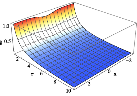
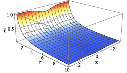
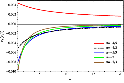
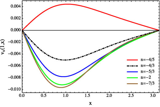
We choose $n=-5/3$ and $n=-4/5$ as two examples for comparisons. Here we make plots for fluid velocity and energy density modified by magnetic fields with $B_{c}^{2}/\epsilon_{c}=0.1$. From Fig.3 and Fig.3 with $n=-5/3$, one finds that the magnetic field yields transverse flow pointing inward into the medium, where the longitudinal flow solely dictated by the Bjorken expansion is not shown here. From Fig.3, one finds that the magnitude of such transverse flow gradually decreases with respect to proper time as expected. In addition, one observes $v_{x}(\tau,0)\approx 0$ since the fluid velocity is only modified by the spatial gradient of magnetic fields. Moreover, the transverse flow is more prominent in the central region with respect to the longitudinal direction as shown in Fig.3. On the contrary, as shown in Fig.5 and Fig.5 with $n=-4/5$, the magnetic field results in the transverse flow pointing outward, whereas other patterns regarding the magnitude of the flow are qualitatively in accordance with the case for $n=-5/3$. Also, as illustrated in Fig.7 and Fig.7, the energy density is most significantly modified in the central region $x\approx 0$, where the reduction is observed in both cases. The change of the direction of the transverse velocity may be anticipated since $v_{x}(\tau,x)=0$ for $n=-1$. In conclusion, the transverse flow led by a Gaussian magnetic field point inward for $n<-1$ and outward for $n>-1$, respectively.

In Fig.9, Fig.9, Fig.11, and Fig.11, we make further comparisons for $v_{x}(\tau,x)$ and $\epsilon_{1}(\tau,x)$ at either fixed $x$ or fixed $\tau$ with different values of $n$ especially for the cases when $n<-1$. Since $v_{x}$ and $\epsilon_{1}$ are even functions with respect to $x$, we only plot the results for $x\geq 0$ in Fig.11 and Fig.11. As shown in Fig.9, when $|n|$ increases for $n<-1$, $|v_{x}|$ at fixed $x$ becomes smaller in late times due to faster decay of the magnetic field. However, the $|v_{x}|$ with larger $|n|$ may increases in early times. In general, there exists no substantial hierarchy of $|v_{x}|$ at fixed $x$ with different values of $n$ in early times. Furthermore, as shown in Fig.11 at $\tau=1$, we find that the $|v_{x}|$ first increase from $x=0$ and then turn over at intermediate $x$ and gradually decrease with $x$. For $n=-4/5$, the velocity profile has a similar shape compared with the cases for $n>-1$, while the direction becomes positive. In contrast, according to Fig.9, the increase of $|\epsilon_{1}|$ at $x=0$ with smaller $|n|$ is observed for almost all times except for $\tau\approx 1$ as further shown in Fig.11. In Fig.11, we find that the correction on energy density could become positive at larger $x$, whereas there exists no clear hierarchy in such a regime. Nonetheless, we should mention the caveat that $v_{x}$ and $\epsilon_{1}$ shown in Fig.11 and Fig.11 are unreliable near $|x|=\pi$, where the approximation of the magnetic field in Fourier series breakdowns. In the fringes $|x|\approx\pi$, the Gaussian function continues decreasing but the Fourier series turnovers as illustrated in Fig.1. In fact, when plotting the $v_{x}$ and $\epsilon_{1}$ at fixed $\tau$ from $x=0$ to $x=2\pi$, we find that $v_{x}$ and $\epsilon_{1}$ becomes odd and even functions with respect to $x=\pi$ since they are formed by sine and cosine series, respectively. We may still conjecture the qualitative behaviors near the fringes based on our approximated solutions. In Fig.11, our approximated solutions of $|v_{x}|$ gradually decreases with $x$ and reach zero at $x=\pi$, while the genuine solutions in principle should decay slower and asymptotically coincide with zero at $x=\infty$. The qualitative behavior of $\epsilon_{1}$ near the fringes is more difficult to analyze because it depends on the competition between $u_{x}$ and $B_{y}$, in which the former causes suppression for $n<-1$ and the latter yields enhancement from the second equation of (5). Note that $u_{x}=-v_{x}$ in our convention and thus $\partial_{\tau}u_{x}$ and $-u_{x}$ are negative for $n>-1$. We may speculate that the effect coming from $u_{x}$ dominates the one from $B_{y}$ for $n<-1$ near the fringes and yields the suppression of $\epsilon_{1}$ in large $|x|$. For $n>-1$, the situation is more oblique, where both $u_{x}$ and $B_{y}$ result in the rise of $\epsilon_{1}$, which may imply the presence of instability near the fringes.

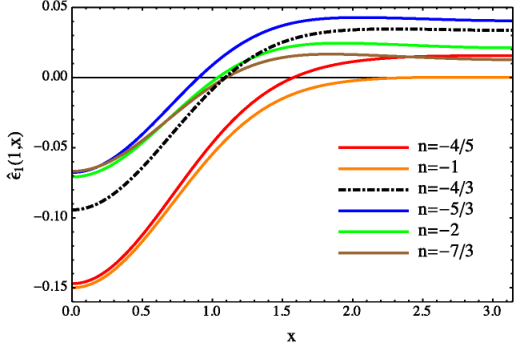
Despite the conjectures of the asymptotic behaviors of the solutions near the fringes, we focus on the central region to qualitatively analyze the physics behind the transverse flow generated by magnetic fields. The change of directions of $v_{x}$ with distinct values of $n$ may be explained by Lenz’s law based on the conservation of magnetic flux. To simplify the conditions, we may consider two extreme cases, which correspond to $n\ll-1$ and $n\gg-1$. For $n\ll-1$, the time scale of the magnetic field is much shorter than the one for the expanding medium, we thus approximate such a condition as a static medium in the presence of a time-decreasing magnetic field $B_{y}(t)$ with a Gaussian distribution in $x$. The total magnetic flux going through the medium now drops with respect to time. The medium is thus pushed inward to the central region $x=0$ in order to preserve the flux. On the contrary, for $n\gg-1$, the magnetic field decays much slower than the expansion of the medium. We thus approximate the situation with the presence of a static magnetic field $B_{y}(x)$ as a Gaussian function of $x$ in a medium expanding along the $z$ direction. In such a case, the total magnetic flux of the medium increases with respect to time. To reduce the flux, the medium hence expands along the $\pm x$ directions. The case for $n=-1$ may correspond to the situation in which the magnetic flux is balanced by the expansion of the medium and the decrease of the magnetic field, which thus results in the absence of transverse flow. Note that the medium here can only change the flux via the expansion or compression in the transverse direction due to the absence of induced electromagnetic fields and currents. On the other hand, the correction on the energy density is affected by both the change of fluid velocity and magnetic field, which varies case by case with different values of $n$. Nevertheless, for the peculiar case $n=-1$, one finds that the decrease of the magnetic field always reduces the energy density.

Before we end this section, we also plot the ratio $B_{y}^{2}/\epsilon$ as a function of $\tau$ for different $n$ and $x$ shown in Fig. 13 and 13, where $\epsilon$ is the total fluid energy density. Since in relativistic heavy ion collisions, the energy density of magnetic fields is expected to decay much faster than the fluid energy density, in Fig. 13 we only plot the case $n<-4/3$. For a smaller value of $n$, i.e. the magnetic field decays faster, the ratio is smaller. Similarly, in Fig. 13 the absolute value of $B_{y}^{2}$ becomes smaller when $x$ increases, but the fluid energy density is approximately homogeneous. Therefore, the ratio reduces when $x$ increases.

In this work, we study a toy model of magnetohydrodynamics in the presence of a transverse external magnetic field with spacetime dependence under the Bjorken expansion. In our setup, the medium is boost-invariant along the $z$ direction and the magnetic field as a function of $\tau$ and $x$ points along the $y$ direction. We obtain the leading-order solutions in the weak-field approximation, where both the energy density and fluid velocity are modified. Particularly, the spatial gradient of the magnetic field engenders transverse flow parallel or anti-parallel to $x$, while the direction and magnitude of flow are determined by the time evolution of the magnetic field. For the magnetic field following power-law decay in proper time such that $|{\bf B}|^{2}\sim\tau^{n}$, the transverse flow propagates inward for $n<-1$ and outward for $n>-1$ based on the conservation of magnetic flux in the expanding medium. The flow vanishes for $n=-1$, which corresponds to the case such that the longitudinal expansion of the medium compensates the decrease of magnetic field. In addition, the energy density is generally reduced in the central region, while it can be enhanced in the outskirts depending on the competing effects between the transverse velocity and the magnetic field.

In general, our study in simple setup may provide better understandings for the influence from spatial gradient of magnetic fields on magnetohydrodynamics. Although we choose the Gaussian distribution as one particular example for the space-dependent magnetic field, the same approach can be applied to other spatial distribution given that the interested regime can be approximated by Fourier decomposition. Since the analytic expressions of each moment is found, one can directly compute the transverse velocity and correction on energy density by just inputting the Fourier coefficients. In the end of conclusions, we would like to reemphasize that this study is a theoretical discussion, which may be far away from phenomenology in heavy ion collisions. Our solutions might be close to the 2+1 dimensional Bjorken flow with transverse magnetic fields near the initial time when the weak-field approximation becomes valid but the transverse flow led by the medium expansion is not fully developed. Here we may further address the validity of our weak-field expansion compared to the practical conditions in heavy ion collisions. According to the numerical simulations [3, 42], the magnetic fields generated in peripheral collisions in RHIC at $\tau=0$ are about $|eB_{y}|\approx 5\sim 10$ $m_{\pi}^{2}$, whereas the magnitudes may drop to ten times smaller at $\tau\approx 0.6$ fm as the onset of hydrodynamic evolution. Assuming the initial temperature of the QGP is about $T_{c}=\epsilon_{c}^{1/4}\approx 300$ MeV, one finds $B_{y}^{2}/\epsilon_{c}\approx 0.17\sim 0.68$ by taking $m_{\pi}\approx 150$ MeV and $e^{2}=4\pi\alpha=4\pi/137$. As a result, the weak-field expansion in our calculations could be a legitimate approximation for the magnetic fields generated in RHIC. It is helpful to use our analytical results to test real numerical MHD in the future.

On the other hand, our study can be generalized along many directions. We may couple the conservation equation to electromagnetic currents, which is essential for analyzing the presence of chemical potential or chiral anomalous effects. To make further connection with heavy ion collisions, the transverse expansion of the medium by itself should be included. The anisotropic flow should be simultaneously affected by the expansion of the medium along both the longitudinal and transverse directions and also the spacetime-varying magnetic field. Furthermore, the viscous effect could be involved as well. How significant the modification from magnetic fields on the flow harmonics measured in experiments is thus relies on the full numerical simulations, which could be affected by the initial conditions chosen for simulations as well. Although the transverse flow led by a inhomogeneous magnetic field shown in this paper is symmetric with respect to the $y$ axis, the flow pattern could become asymmetric from an asymmetric distribution of $B_{y}$ or the presence of $B_{x}$. Based on the event-by-event fluctuations [3], the magnitude of $B_{x}$ could be comparable with the magnitude of $B_{y}$. Consequently, except for the even harmonics, the flow engendered by spatial inhomogeneity of magnetic fields may possibly affect the odd harmonics in heavy ion collisions as well. On the other hand, in order to gain more insights for the early-time physics, one may have to seek the next leading-order solutions to incorporate nonlinear effects of strong magnetic fields.

S.P. is supported by the Alexander von Humboldt Foundation, Germany and D.Y. is supported by the RIKEN Foreign Postdoctoral Researcher program.

References

- [1] M. Gyulassy and L. McLerran, Nucl. Phys. A750, 30 (2005), eprint nucl-th/0405013.
- [2] A. Bzdak and V. Skokov, Phys.Lett. B710, 171 (2012), eprint 1111.1949.
- [3] W.-T. Deng and X.-G. Huang, Phys.Rev. C85, 044907 (2012), eprint 1201.5108.
- [4] K. Tuchin, Phys.Rev. C83, 017901 (2011), eprint 1008.1604.
- [5] G. Basar, D. Kharzeev, D. Kharzeev, and V. Skokov, Phys.Rev.Lett. 109, 202303 (2012), eprint 1206.1334.
- [6] S.-Y. Wu and D.-L. Yang, JHEP 08, 032 (2013), eprint 1305.5509.
- [7] B. Muller, S.-Y. Wu, and D.-L. Yang, Phys. Rev. D89, 026013 (2014), eprint 1308.6568.
- [8] D.-L. Yang and B. Muller, J. Phys. G39, 015007 (2012), eprint 1108.2525.
- [9] C. S. Machado, F. S. Navarra, E. G. de Oliveira, J. Noronha, and M. Strickland, Phys. Rev. D88, 034009 (2013), eprint 1305.3308.
- [10] J. Alford and M. Strickland, Phys.Rev. D88, 105017 (2013), eprint 1309.3003.
- [11] X. Guo, S. Shi, N. Xu, Z. Xu, and P. Zhuang, Phys. Lett. B751, 215 (2015), eprint 1502.04407.
- [12] K. Fukushima, K. Hattori, H.-U. Yee, and Y. Yin (2015), eprint 1512.03689.
- [13] D. E. Kharzeev, L. D. McLerran, and H. J. Warringa, Nucl.Phys. A803, 227 (2008), eprint 0711.0950.
- [14] K. Fukushima, D. E. Kharzeev, and H. J. Warringa, Phys.Rev. D78, 074033 (2008), eprint 0808.3382.
- [15] D. E. Kharzeev and H.-U. Yee, Phys.Rev. D83, 085007 (2011), eprint 1012.6026.
- [16] Y. Burnier, D. E. Kharzeev, J. Liao, and H.-U. Yee, Phys.Rev.Lett. 107, 052303 (2011), eprint 1103.1307.
- [17] M. Stephanov and Y. Yin, Phys.Rev.Lett. 109, 162001 (2012), eprint 1207.0747.
- [18] J.-W. Chen, J.-y. Pang, S. Pu, and Q. Wang, Phys.Rev. D89, 094003 (2014a), eprint 1312.2032.
- [19] J.-Y. Chen, D. T. Son, M. A. Stephanov, H.-U. Yee, and Y. Yin, Phys.Rev.Lett. 113, 182302 (2014b), eprint 1404.5963.
- [20] D. T. Son and N. Yamamoto, Phys.Rev.Lett. 109, 181602 (2012), eprint 1203.2697.
- [21] D. T. Son and N. Yamamoto, Phys.Rev. D87, 085016 (2013), eprint 1210.8158.
- [22] J.-H. Gao, Z.-T. Liang, S. Pu, Q. Wang, and X.-N. Wang, Phys.Rev.Lett. 109, 232301 (2012), eprint 1203.0725.
- [23] J.-W. Chen, S. Pu, Q. Wang, and X.-N. Wang, Phys.Rev.Lett. 110, 262301 (2013), eprint 1210.8312.
- [24] A. Bzdak, V. Koch, and J. Liao, Lect.Notes Phys. 871, 503 (2013), eprint 1207.7327.
- [25] D. E. Kharzeev, Prog.Part.Nucl.Phys. 75, 133 (2014), eprint 1312.3348.
- [26] D. E. Kharzeev (2015), eprint 1501.01336.
- [27] X.-G. Huang and J. Liao, Phys.Rev.Lett. 110, 232302 (2013), eprint 1303.7192.
- [28] S. Pu, S.-Y. Wu, and D.-L. Yang, Phys.Rev. D89, 085024 (2014), eprint 1401.6972.
- [29] Y. Jiang, X.-G. Huang, and J. Liao, Phys.Rev. D91, 045001 (2015), eprint 1409.6395.
- [30] S. Pu, S.-Y. Wu, and D.-L. Yang, Phys.Rev. D91, 025011 (2015), eprint 1407.3168.
- [31] P. Romatschke and U. Romatschke, Phys. Rev. Lett. 99, 172301 (2007), eprint 0706.1522.
- [32] M. Luzum and P. Romatschke, Phys. Rev. C78, 034915 (2008), eprint 0804.4015.
- [33] H. Song and U. W. Heinz, Phys.Lett. B658, 279 (2008a), eprint 0709.0742.
- [34] H. Song and U. W. Heinz, Phys. Rev. C78, 024902 (2008b), eprint 0805.1756.
- [35] B. Schenke, S. Jeon, and C. Gale, Phys. Rev. C85, 024901 (2012), eprint 1109.6289.
- [36] V. Roy, A. K. Chaudhuri, and B. Mohanty, Phys. Rev. C86, 014902 (2012), eprint 1204.2347.
- [37] H. Niemi, G. S. Denicol, P. Huovinen, E. Molnar, and D. H. Rischke, Phys. Rev. C86, 014909 (2012), eprint 1203.2452.
- [38] K. Tuchin, Phys.Rev. C88, 024911 (2013), eprint 1305.5806.
- [39] U. Gursoy, D. Kharzeev, and K. Rajagopal, Phys. Rev. C89, 054905 (2014), eprint 1401.3805.
- [40] B. G. Zakharov, Phys. Lett. B737, 262 (2014), eprint 1404.5047.
- [41] H. Li, X.-l. Sheng, and Q. Wang (2016), eprint 1602.02223.
- [42] V. Roy and S. Pu (2015), eprint 1508.03761.
- [43] L. D. Landau, Izv. Akad. Nauk Ser. Fiz. 17, 51 (1953).
- [44] J. D. Bjorken, Phys. Rev. D27, 140 (1983).
- [45] S. S. Gubser, Phys. Rev. D82, 085027 (2010), eprint 1006.0006.
- [46] S. S. Gubser and A. Yarom, Nucl. Phys. B846, 469 (2011), eprint 1012.1314.
- [47] Y. Hatta, J. Noronha, and B.-W. Xiao, Phys. Rev. D89, 114011 (2014a), eprint 1403.7693.
- [48] Y. Hatta, J. Noronha, and B.-W. Xiao, Phys. Rev. D89, 051702 (2014b), eprint 1401.6248.
- [49] Y. Hatta, J. Noronha, G. Torrieri, and B.-W. Xiao, Phys. Rev. D90, 074026 (2014c), eprint 1407.5952.
- [50] L.-G. Pang, Y. Hatta, X.-N. Wang, and B.-W. Xiao, Phys. Rev. D91, 074027 (2015), eprint 1411.7767.
- [51] Y. Hatta, B.-W. Xiao, and D.-L. Yang, Phys. Rev. D93, 016012 (2016), eprint 1512.04221.
- [52] V. Roy, S. Pu, L. Rezzolla, and D. Rischke (2015), eprint 1506.06620.
- [53] L. Rezzolla and O. Zanotti, Relativistic Hydrodynamics (Oxford University Press, 2013).
- [54] L. Landau and E. M. Lifshitz, Fluid dynamics (Pergamon, New York, 1959).
- [55] S. Pu, V. Roy, L. Rezzolla, and D. H. Rischke (2016), eprint 1602.04953.
- [56] L.-g. Pang, G. Endrődi, and H. Petersen (2016), eprint 1602.06176.
- [57] M. Gedalin and I. Oiberman, Phys. Rev. E 51, 4901 (1995), URL http://link.aps.org/doi/10.1103/PhysRevE.51.4901.
- [58] X.-G. Huang, M. Huang, D. H. Rischke, and A. Sedrakian, Phys. Rev. D81, 045015 (2010), eprint 0910.3633.