Parallel Linear Search with no Coordination
for a Randomly Placed Treasure
Abstract
In STOC’16, Fraigniaud et al. consider the problem of finding a treasure hidden in one of many boxes that are ordered by importance. That is, if a treasure is in a more important box, then one would like to find it faster. Assuming there are many searchers, the authors suggest that using an algorithm that requires no coordination between searchers can be highly beneficial. Indeed, besides saving the need for a communication and coordination mechanism, such algorithms enjoy inherent robustness. The authors proceed to solve this linear search problem in the case of countably many boxes and an adversary placed treasure, and prove that the best speed-up possible by non-coordinating searchers is precisely . In particular, this means that asymptotically, the speed-up is four times worse compared to the case of full coordination.
We suggest a natural variant of the problem, where the treasure is placed uniformly at random in one of a finite, large, number of boxes. We devise non-coordinating algorithms that achieve a speed-up of for two searchers, a speed-up of for three searchers, and in general, a speed-up of for any searchers. Thus, as grows to infinity, the speed-up approaches three times worse compared to the case of full coordination. Moreover, these bounds are tight in a strong sense as no non-coordinating search algorithm for searchers can achieve better speed-ups. We also devise non-coordinating algorithms that use only logarithmic memory in the size of the search domain, and yet, asymptotically, achieve the optimal speed-up. Finally, we note that all our algorithms are extremely simple and hence applicable.
1 Introduction
Parallel algorithms are often evaluated by their speed-up, which measures how much faster the parallel algorithm with processors runs in comparison to the best running time that a single processor can achieve. In [13], the authors focused on parallel non-coordinating algorithms. In such an algorithm, all processors operate independently, by executing the same protocol, differing only in the outcome of the flips of their random coins. A canonical example is the case of multiple random walkers that search in a graph [1]. Although most problems cannot be efficiently parallelized without coordination, when such parallelization can be achieved, the benefit can potentially be high. Particularly, as argued in [13], the gain can be not only in terms of saving in communication and overhead in computation, but also in terms of robustness.
One class of fundamental problems that enjoys a large non-coordination ratio in some circumstances, is the class of search problems over totally ordered sets. The objective of such linear search problems is to find a solution among a set of candidate solutions that are linearly ordered according to their quality. For instance, searching for a proper divisor of a random integer is an illustration of linear search. In this case, enumerating the candidate divisors in increasing order, and checking them one after another, is the typical strategy to solve the problem, as the probability that is divisible by a given prime is inversely proportional to this prime. Similarly, in cryptography, an exhaustive search attack is better proceeded by systematically checking smaller keys than longer ones, since checking a key typically requires exponential time in the key size. In general, linear search appears in contexts in which the search space can be ordered in a way such that, given that the previous trials failed, the next candidate according to the order is either the most likely to be valid, or most preferable, or the easiest to check.
One basic linear search problem is the treasure-hunt problem. There is one treasure hidden in one box out of a linearly ordered set of boxes . Searchers are unaware of the index and their goal is to find the treasure as fast as possible. At each time step, a protocol executed by a searcher has the ability to peek into one box and see whether the treasure is present or not in that box. The protocol is terminated once one of the searchers finds the treasure. Boxes are listed in an order that reflects the importance of finding the treasure in a given box. That is, finding the treasure hidden in for small values of is more urgent than for large values of . In the case of a solo searcher, the best strategy is to open the boxes in increasing order. In this case, the searcher will find the treasure in time. Hence, for a given algorithm , we measure the speed-up function of searchers with respect to as:
where the expectation is taken with respect to the randomness of the searchers. Note that if coordination is allowed, one could simply divide the set of boxes evenly between the searchers leading to a speed-up of . However, as mentioned in [13], as simple as this algorithm is, it is very sensitive to faults of all sorts. For example, if one searcher crashes at some point in time during the execution then the searchers may completely miss the treasure, unless the protocol employs some mechanism for detecting such faults. This observation motivates the study of non-coordinating algorithms.
In [13] the authors considered the case in which an adversary places the treasure in one of infinitely countable boxes. In this case, for any non-coordinating algorithm, the adversary can always find a box for which the speed-up would be at most 1. Therefore, the speed-up of an algorithm was defined as . They then present Algorithm 1 that is very simple and achieves optimal performance, a speed-up of for each . Specifically, the speed-up is for two searchers, for three searchers, and roughly for searchers as grows larger. It is shown that no non-coordinating search algorithm can achieve better speed-ups.
In this paper, we expand on the techniques and results of [13], and solve a natural variant of the treasure-hunt problem. In our scenario, the treasure is placed at random in one of boxes. We therefore define the speed-up of an algorithm as:
where the expectation is taken with respect to the placement of . The speed-up of agents on boxes is defined as the speed-up of the best algorithm for boxes. That is:
Finally, the general speed-up of agents is defined as the speed-up of the best algorithm for boxes, where is taken to infinity. That is:
1.1 Our Results
We suggest a general framework to tackle the randomly placed treasure hunt problem and solve it completely for the case of a treasure uniformly placed in one of finitely many boxes.
Specifically, we prove that the optimal speed-up for non-coordinating algorithms running with searchers is:
This means that the best speed-up that can be achieved is for two searchers, for three searchers, and roughly for searchers, as grows larger. We stress that these bounds are tight in a strong sense as no non-coordinating search algorithm for searchers can achieve better speed-ups, for any .
Our results indicate that the best possible speed-up for the random setting is strictly higher than the best possible speed-up for the adversarial setting. Specifically, as the number of searchers grows, the multiplicative gap between the settings approaches .
The non-coordinating algorithm achieving11 1 Note that this algorithm achieves the bound in an asymptotic manner, meaning that as the number of boxes goes to infinity, the speed-up of the algorithm approaches the desired bound. For small number of boxes there might be better algorithms. the aforementioned ratio for the random setting with searchers is so simple that it can be described in just a few lines (Algorithm 2). Note that for each and the algorithm is different.
It is interesting to note that this algorithm finds a way to balance between two opposing forces: it gives higher probability of quickly opening the more important boxes, and yet tries to minimize as much as possible the overlap between different agents.
Despite the simplicity of Algorithm 2, finding it was not an easy task. Indeed, there are many possible algorithms that achieve an speed-up, but coming up with an algorithm that has an exact optimal bound is not trivial. This is especially challenging as every slight change in the algorithm may significantly complicate its analysis.
Algorithm 2 achieves optimal speed-up for each but requires bits of memory to store the elements that have already been checked. To circumvent this, we suggest and analyse a natural variant of this algorithm, which works in exactly the same fashion, except that it does not remember the boxes it already checked. It therefore requires only bits of memory, and yet its speed-up is , which is practically the same as that of the optimal algorithm for large .
Concerning the technical aspects, in a similar fashion to [13], we first observe that the crucial aspects of non-coordinating algorithms can be represented by matrices and then approximate matrices by continuous functions. To show the upper bound on the speed-up we had to upper bound the integral of functions satisfying certain restrictions. As in [13], the biggest technical challenges lie in computing such integrals. This task turned out to be more difficult than in the adversarial case of [13], and we were therefore unable to directly compute these integrals. Instead, to overcome this, we needed two new tools: We extend a lemma of [13] to work on unbounded functions, and introduce the intuitive notion of the “zooming” of a function. Using this two new results, we can reduce the problem to solving simpler integrals. We then turn to analyze Algorithm 2 to lower bound the speed-up for agents. One of the problems arising in the analysis of Algorithm 2which did not occur in the limsup adversarial setting of [13], is that the first boxes cannot be ignored, as they contribute significantly to the average case analysis. To overcome this we prove a small, yet useful, result regarding the Gamma function.
As mentioned, we fully characterize the case of a treasure placed uniformly at random. We note, however, that the general framework of analysis presented in this paper could be useful in order to derive speed-up bounds with respect to other distributions as well. Handling other distributions, however, would require solving the corresponding particular integrals.
To sum up, our upper bound on the speed-up of non-coordination algorithms implies that there is a price to be paid for the absence of coordination, which is asymptotically a factor of three away from an ideal optimal algorithm that performs with perfect coordination. On the other hand, this price is actually reasonably low, and so in faulty contexts in which coordination between the searchers may yield severe overheads, it might well be worth giving up on coordination, and simply run our non-coordinating algorithm.
1.2 Related Work
Most of the parallel search literature deals with mobile agents searching graphs of different topologies. One example is search by multiple random walkers. In a series of papers [1, 5, 8, 7] several results regarding hitting time, cover time and mixing times are established, such as a linear speed-up for several graph families including expanders and random graphs.
Another classical example of mobile search is the linear search problem [3, 4] (and later [14]), where a treasure is hidden on the real line according to a known probability distribution. A searcher starts from the origin and wishes to discover the treasure in minimal expected time. This problem was reintroduced by computer scientists as the cow-path problem [2, 15]. There, similarly to this paper, the time complexity is measured as a function of the distance of the treasure from the starting point.
Motivated by applications to central search foraging by desert ants, the authors in [11, 12] considered the ANTS problem, a variant of the cow-path problem on the grid, and showed that a speed-up of can be achieved with independent searchers. Several variants of the cow-path problem and the ANTS problem were studied in [6, 9, 10, 16, 17, 18].
The major difference between our setting and the mobile agent setting, is that we allow “random access” to the different boxes. That is, our searcher can jump between different boxes at no cost, unlike the case of mobile agents on a graph which can only move from a vertex to a neighboring vertex in one time step.
2 Preliminaries
In this section we go over the setup of [13] with some minor changes that reflect our changed definition of speed-up. We then proceed to introduce some new tools to help us deal with the case of randomly placed treasure.
2.1 Setup
Our universe contains boxes indexed by , and a treasure that is placed uniformly at random in one of them. At each time step, a searcher can peek into exactly one box. There are searchers and they are all completely identical in that they have the same algorithm, yet their randomness is independent. They do not communicate at all, and their mutual purpose is to maximize the speed-up by minimizing the expected time until the first one of them finds the treasure. In our technical discussion it will be often easier to work with the inverse of the speed-up. Specifically, for an algorithm and an index , define:
where the expectation is taken over the randomness of the searchers. Taking expectation over the placement of , we define:
So, an algorithm with means that running this algorithm on three searchers will result in an expected running time that is twice as fast as the trivial one-searcher algorithm.
2.2 From Algorithms to Matrices
Given an algorithm, we define the matrix , where is the probability that the algorithm executed with just one searcher has not visited box up to (and including) step . For example, the following matrix corresponds to Algorithm 2, where and (note that we stop after time since afterwards, the matrix is all 0’s).
Some observations:
- 1.
The value of is multiplied by the probability that will not be checked at time . This is how we arrived at the matrix above.
- 2.
The sum of row is the expected time until the algorithm peeks into box . Indeed, let denote the indicator random variable that is 1 iff the visit time of . The sum of these over is the visit time. Also, , so we get the result by linearity of expectation. This means:
- 3.
Given the matrix for one searcher, what would be the matrix for searchers? The probability of not being looked into up to step is the probability that all searchers didn’t peek into it, which is . So by the same reasoning as the last point, we get:
(1) - 4.
Since is the probability that box was peeked into by step , summing these numbers over column , we get the expected number of boxes checked by this time, which is of course at most . Denoting:
The column requirement is that for all , . The matrix resulting from an algorithm will always satisfy the column requirement.
2.3 One Searcher
A simple and intuitive result is when considering just one agent. We show it here for completeness and also as intuition, as it is a very simple version of the proof for the general case.
Theorem 1.
.
Proof.
The algorithm that opens one box after another will take time to find the treasure if it is in box , and so: , meaning that . So, .
On the other hand, take some algorithm and denote its matrix by .
| (2) |
We aim to show that . For this purpose, we actually show that this inequality holds for every taking values in satisfying the column requirement. That is, we know that for every ,
Wanting to minimize (2) under this restriction means that we can deal with each column separately. So the question is, given some integer , what are the values of that minimize under the restriction that . The answer is for all and for the others. Otherwise there is some , s.t. one can decrease a little and increase by the same amount. This will result in a smaller sum without violating the constraint.
The resulting optimal matrix is therefore for all and otherwise. This is exactly the matrix of the trivial algorithm, and so the optimal speedup is at most . ∎
2.4 From Matrices to Functions
It will be much easier to work with a continuous version of our problem. For an interval denote: . For an , we say that satisfies the column requirements if for all :
We call such a function valid, and denote by the set of all such valid functions. We define:
where we can change the integral because of Tonelli’s theorem. The following claim shows a connection between matrices and functions:
Claim 1.
For any algorithm that works on boxes, there is a function such that for all , .
The proof is in Appendix A.1, where we choose to be a continuous version of the step function derived from ’s matrix.
Claim 1 shows that upper bounding the speed-up of all functions in will upper bound the speed-up of all algorithms on boxes.
3 Zooming in (or out) a Function
We introduce a new and important tool that will be used a couple of times in what proceeds. If we have some algorithm that works for boxes, we would like to be able to use it on boxes. Slowing it down by a factor of two, and using the extra probability to cover the extra boxes can do the trick. How to do this for algorithms is not clear, but for continuous functions it is simple and elegant.
Definition 1.
Given some and some , we define the zooming of by as:
Where .
The intuitive meaning of it is that we expanded the algorithm to work on a domain of size times the original one, and slowed it down by a factor of . What happens to the column integrals and to the speed-up?
Claim 2.
For and , we have and for all values , .
Proof.
The inverse speed-up:
And the column integrals:
∎
Corollary 1.
For and any , we have that and has exactly the same speed-up as .
Proof.
By Claim 2 and the fact that satisfies the column requirements, . By the same claim we see that the speedup remains unchanged. ∎
4 Upper Bound
Theorem 2.
For all :
To prove the theorem, we show that for every , for large enough , any algorithm working on boxes satisfies:
The case was dealt with in Section 2.3. Claim 1 says that if we prove this for all then we have proved it on all algorithms designed for boxes. Corollary 1 then says that by zooming by , proving the following claim will prove Theorem 2:
Claim 3.
There is some real function , s.t. , and every satisfies:
We use a lemma22 2 It is slightly changed here: the upper bound of the domain is 1 and not infinity. This changes nothing in the original proof and actually simplifies the statement of the lemma, as boundedness and integrability of are immediate. We also change the requirement to inequality, and this again, changes nothing, as when the optimal solution is not 0, it will clearly take the equality. of [13]:
Lemma 1.
Fix and . For continuous functions and where , the minimum of , ranging over all possible ’s is achieved when
where is a function of and , and independent of .
This lemma is exactly what we need to prove Claim 3. Informally, considering , the column requirement is the condition on in the lemma, just setting , and by plugging in , we get the form of the optimal function for each of the columns. For each , we then find the maximal solving , and thus get the optimal function for a specific . We can then calculate and take the limit as goes to 0 (that is, goes to infinity) to get our result.
The only problem with this approach is that the integrals become difficult to solve when we start them at some arbitrary . We therefore take . Then, as we shall see, the integrals are pretty straightforward. Our plan is therefore as follows:
- 1.
Extend Lemma 1. This is because it doesn’t work now, as is not defined on , and cannot be extended in a continuous way to it.
- 2.
Use the extended lemma to find the exact optimal function in the case of , and calculate its speed-up.
- 3.
Use the result to come back to with asymptotically insignificant change in speed-up.
This is the extended lemma:
Lemma 2.
Fix . For continuous functions and where is defined and , the minimum of , ranging over all possible ’s is achieved when:
Where is a function of and , and independent of .
It is proved in Appendix A.2 by using the original lemma on subsets , taking the limit of the resulting functions, and then using the dominated convergence theorem.
As we can see the condition on is a bit bizarre, but it proves what we need:
Corollary 2.
Among all continuous functions satisfying , the one that minimizes is , where is a function of .
Proof.
Set . To use Lemma 2, we check that , and this is true for all . ∎
4.1 The Optimal Function
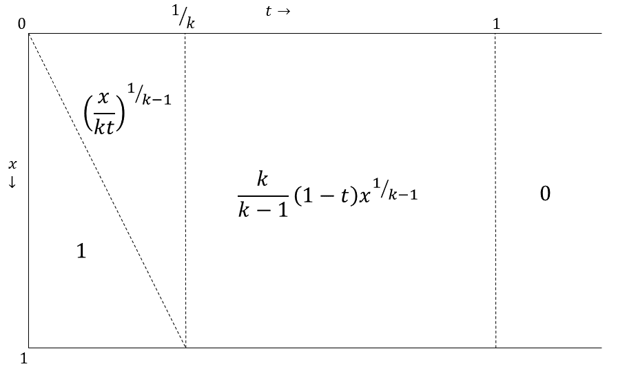

Claim 4.
, and every satisfies . Also,
4.2 And now with
The following claim is what we need to conclude the upper bound proof and prove Claim 3:
Claim 5.
There is some real function , s.t. , and every satisfies .
Proof.
We construct a new function that will span the whole range of ’s from to , with little change to . This will be done by slowing down, and using what we saved in the column integrals to visit the ’s between and using our optimal solution, running it fast enough so it does not incur a big difference in .
Fix some to be determined later. Define:
Since the zoomed version of here is defined on the ’s in and the zoomed is on those in , we get that for all :
where we used Claim 2 and the fact that both and satisfy the column requirements.
5 Matching Lower Bound
In this section we prove:
Theorem 3.
For all :
The case of was dealt with in Section 2.3. For , denote by , Algorithm 2 when set to run with parameter and . To prove Theorem 3, we prove:
Claim 6.
For every ,
Proof.
Denote the matrix of by . A general observation is that:
Since the algorithm chooses uniformly from a set of unopened boxes at each stage, this is:
Applying generously we get:
where we assumed is a multiple of . Otherwise, take large enough and round it up to be a multiple of , the few extra boxes will not change the speed-up. Also, note that the value of where is not a multiple of is the same as that of where is the next multiple of greater than . We can therefore calculate the double sum of , when summing only over ’s that are multiples of , and multiply the result by . From here on we will assume is a multiple of .
We will need the following lemma:
Lemma 3.
For integers , and , .
Using properties of the Gamma function it is easy to see that the two sides of the equation are asymptotically equal, but this is not enough to prove our result as we need the inequality for small and as well. We prove this Lemma in Appendix A.4. Now:
And:
So finally:
This is strangely familiar. Looking at (3) we notice that:
Calculating the sums of is like approximating the double integral of , and as goes to infinity this approximation can be as close as we wish. A fine detail is with the fact that we take only ’s that are multiples of , but this creates a factor in the sum approximating the integral which is then cancelled by multiplying the total sum by , as said above. ∎
5.1 Algorithm with memory
As it is now, Algorithm 2 uses a lot of memory. Each searcher needs to remember all of the boxes it checked, so we need memory in the worst case. However, if we are willing to lose a little in the speed-up, we can save a lot in memory.
Algorithm 3 is exactly the same as Algorithm 2, except it doesn’t remember where it’s been. The only memory it uses is the counter, and so it needs only bits of memory. Denote by , Algorithm 3 when set to run with parameter and . In Appendix A.5 we prove:
Claim 7.
As we can see, this algorithm, for large and will have essentially the same speed-up as that of the optimal algorithm while using exponentially less memory.
Appendix A Appendix
A.1 Proof of Claim 1
Claim 1.
For any algorithm that works on boxes, there is a function such that for all , .
Proof.
Given , take its matrix , and define . For any :
So satisfies the column requirements. Next, let us upper-bound the inverse of the speed-up.
where the inequality is because and . is a step function and not continues but can be turned into a continues function with as little change in integral as we wish - we can leverage what we gain in the inequality above to account for this change. ∎
A.2 Proof of the Extended Lemma
Lemma 2.
Fix . For continuous functions and where is defined and , the minimum of , ranging over all possible ’s is achieved when:
Where is a function of and , and independent of .
Proof.
First, note that if then the optimal solution is and then . Otherwise, and this hold for Lemma 1 as well, we can assume that the constraint is actually an equality, as maximizing it will always decrease the target integral.
For each , applying Lemma 1, there is some such that among all functions , satisfying (again, since , this is actually an equality), the function:
Minimizes .
Extend each to be also defined on by setting it to be there. Since is derived as the solution to:
We can see that as decreases, decreases, and as the are bounded below by , they converge to some . Denote .
Clearly, the converge point-wise to as approaches . By the bounded convergence theorem we get:
Since decreases as decreases, we get that for all :
By our requirements on we know that , so by the dominated convergence theorem we can exchange integral and limit and get:
| (4) |
Now, assume there is some satisfying the conditions that is better than . That is:
| (5) |
We take an small enough so that (4) is more than close to the limit, and we get:
Yet we know that is optimal on and since it is on , cannot be better. so this latter sum is at least contradicting (5). ∎
A.3 Optimality of
Claim 4.
, and any has . Also,
Proof.
Corollary 2 gives for each fixed the function minimizing . Setting will give the minimal , which is the goal.
All we have to do is figure out . First, for , the optimal is obviously , since this satisfies the column requirement and contributes to our target double integral. For , we have , and that . So, given , we figure out what its is. For each , denote by (a function of ) the smallest where , and in case this does not happen, set :
| (6) |
for every , satisfies the column requirement , and since it minimizes the target integral, it will actually be an equality:
We have two cases:
- 1.
for all where this equation is:
From (6), we get . Plugging this in:
So:
This means, that for all , and then . For all other , .
- 2.
for all where :
and so:
Putting all this together gives us as in (3).
Now we can calculate :
We focus on each one of these:
- 1.
Here we know that .
We get:
The whole integral:
- 2.
Here, still, .
Plugging our in, and calculating the whole integral:
Last bit is because indefinite integral of is .
- 3.
Here .
plugging in our and calculating the whole integral:
In total we get:
∎
A.4 Proof of the Gamma Function Property
Lemma 3.
For integers , and ,
Proof.
By induction on (somehow on it doesn’t work..). If , then we should show , which is true. We therefore assume that the result holds for and prove it for :
We want to show:
Take and the above is equivalent to:
If we show that the left side is increasing with when then we are done. We take the derivative (using an internet site):
This is positive if
Take . We want to show that
We use the equality
So
as desired. ∎
A.5 Speedup of Algorithm 3
Claim 7.
Proof.
By the same reasoning as the original algorithm, the matrix of this one is:
Using Lemma 3:
Using it and ignoring all the rounding, as in the analysis of Algorithm 2:
To upper bound , we calculate each area of the sum separately. In what follows, we use the fact that is large for a few approximations.
- 1.
The ’s contribute:
- 2.
The second part contributes:
where the double sum is equal to , by noting that appears there once, appear twice, and so on.
- 3.
The last part is:
Putting it all together, we get the result. ∎
References
- [1] Noga Alon, Chen Avin, Michal Koucky, Gady Kozma, Zvi Lotker, and Mark R. Tuttle. Many Random Walks Are Faster Than One. In Proceedings of the Twentieth Annual Symposium on Parallelism in Algorithms and Architectures, SPAA ’08, pages 119–128, New York, NY, USA, 2008. ACM.
- [2] R.A. Baezayates, J.C. Culberson, and G.J.E. Rawlins. Searching in the Plane. Inf. Comput., 106(2):234–252, October 1993.
- [3] Anatole Beck. On the linear search problem. Israel Journal of Mathematics, 2(4):221–228, 1963.
- [4] Richard Bellman. An Optimal Search. SIAM Review, 5(3):274–274, 1963.
- [5] Colin Cooper, Alan M. Frieze, and Tomasz Radzik. Multiple Random Walks in Random Regular Graphs. SIAM J. Discrete Math., 23(4):1738–1761, 2009.
- [6] Erik D. Demaine, Sándor P. Fekete, and Shmuel Gal. Online searching with turn cost. Theor. Comput. Sci., 361(2-3):342–355, 2006.
- [7] Klim Efremenko and Omer Reingold. How Well Do Random Walks Parallelize? In Irit Dinur, Klaus Jansen, Joseph Naor, and José Rolim, editors, Approximation, Randomization, and Combinatorial Optimization. Algorithms and Techniques: 12th International Workshop, APPROX 2009, and 13th International Workshop, RANDOM 2009, Berkeley, CA, USA, August 21-23, 2009. Proceedings, pages 476–489. Springer Berlin Heidelberg, Berlin, Heidelberg, 2009.
- [8] Robert Elsässer and Thomas Sauerwald. Tight bounds for the cover time of multiple random walks. Theor. Comput. Sci., 412(24):2623–2641, 2011.
- [9] Yuval Emek, Tobias Langner, David Stolz, Jara Uitto, and Roger Wattenhofer. How many ants does it take to find the food? Theor. Comput. Sci., 608:255–267, 2015.
- [10] Yuval Emek, Tobias Langner, Jara Uitto, and Roger Wattenhofer. Solving the ANTS Problem with Asynchronous Finite State Machines. In Automata, Languages, and Programming - 41st International Colloquium, ICALP 2014, Copenhagen, Denmark, July 8-11, 2014, Proceedings, Part II, pages 471–482, 2014.
- [11] Ofer Feinerman and Amos Korman. Memory Lower Bounds for Randomized Collaborative Search and Implications for Biology. In Distributed Computing - 26th International Symposium, DISC 2012, Salvador, Brazil, October 16-18, 2012. Proceedings, pages 61–75, 2012.
- [12] Ofer Feinerman, Amos Korman, Zvi Lotker, and Jean-Sébastien Sereni. Collaborative search on the plane without communication. In ACM Symposium on Principles of Distributed Computing, PODC ’12, Funchal, Madeira, Portugal, July 16-18, 2012, pages 77–86, 2012.
- [13] Pierre Fraigniaud, Amos Korman, and Yoav Rodeh. Parallel Exhaustive Search without Coordination. CoRR, abs/1511.00486, 2015. To appear in STOC 2016.
- [14] Shmuel Gal. Minimax Solutions for Linear Search Problems. SIAM Journal on Applied Mathematics, 27(1):17–30, 1974.
- [15] Ming-Yang Kao, John H. Reif, and Stephen R. Tate. Searching in an Unknown Environment: An Optimal Randomized Algorithm for the Cow-path Problem. In Proceedings of the Fourth Annual ACM-SIAM Symposium on Discrete Algorithms, SODA ’93, pages 441–447, Philadelphia, PA, USA, 1993. Society for Industrial and Applied Mathematics.
- [16] Richard M. Karp, Michael E. Saks, and Avi Wigderson. On a Search Problem Related to Branch-and-Bound Procedures. In 27th Annual Symposium on Foundations of Computer Science, Toronto, Canada, 27-29 October 1986, pages 19–28, 1986.
- [17] Tobias Langner, Jara Uitto, David Stolz, and Roger Wattenhofer. Fault-Tolerant ANTS. In Distributed Computing - 28th International Symposium, DISC 2014, Austin, TX, USA, October 12-15, 2014. Proceedings, pages 31–45, 2014.
- [18] Christoph Lenzen, Nancy A. Lynch, Calvin C. Newport, and Tsvetomira Radeva. Trade-offs between selection complexity and performance when searching the plane without communication. In ACM Symposium on Principles of Distributed Computing, PODC ’14, Paris, France, July 15-18, 2014, pages 252–261, 2014.