Option Pricing in Markets with Unknown Stochastic Dynamics
Abstract
We consider arbitrage free valuation of European options in Black-Scholes and Merton markets, where the general structure of the market is known, however the specific parameters are not known. In order to reflect this subjective uncertainty of a market participant, we follow a Bayesian approach to option pricing. Here we use historic discrete or continuous observations of the market to set up posterior distributions for the future market. Given a subjective physical measure for the market dynamics, we derive the existence of arbitrage free pricing rules by constructing subjective option pricing measures. The non-uniqueness of such measures can be proven using the freedom of choice of prior distributions. The subjective market measure thus turns out to model an incomplete market. In addition, for the Black-Scholes market we prove that in the high frequency limit (or the long time limit) of observations, Bayesian option prices converge to the standard BS-Option price with the true volatility. In contrast to this, in the Merton market with normally distributed jumps Bayesian prices do not converge to standard Merton prices with the true parameters, as only a finite number of jump events can be observed in finite time. However, we prove that this convergence holds true in the limit of long observation times.
Key words: Bayesian arbitrage free option pricing, Bayes statistics, Bayesian consistency
Mathematics Subject Classification (2010) 91G20, 62F15
1 Introduction
We consider the thought experiment, where a market participant prices options based on a market model for the underlying asset where the market’s general structure is known as, however the model parameters are not known. The models considered here are the Black-Scholes [2, 18] (pure exponential diffusion) and Merton [19] (exponential jump diffusion) models. The calibration of the parameters is based on discrete (low frequency) or continuous (high frequency) observations of in the time preceding interval , where is the observation time. So we deal with historical volatility for the Black Scholes model and historical jump frequency and height distribution for the Merton model. Furthermore, the market participant follows an Bayesian approach in order to express her or his uncertainty about the parameters of the underlying model . Hence, the subjective market measure for the market is a mixture of the parametric family of market measures with respect to the model parameters and with weights given by a posterior distribution .
The main results of this paper are the following: First, we prove that for the Black-Scholes and Merton markets arbitrage free pricing rules (or equivalent martingale measures) exist and can be obtained as a mixture from a parameter-dependent family of equivalent martingale measures . As in the definition of does not necessarily have to be the same posterior distribution as in the definition of , while remains to be an equivalent martingale measure with respect to as long as both posterior distributions are equivalent, we conclude that subjective markets are incomplete even in the case where the corresponding market for a fixed set of the parameters is a complete market, as in the case of the Black-Scholes market. Although this result seems to be rather natural, a proof seems to be missing in the literature.
Second, we prove that the option prices for European options obtained by the pricing measure converge almost surely to the Black-Scholes prices in the limit of high frequency observations or long time observations at a given frequency. We give a complete proof for this result for normalizable and non normalizable prior distributions using a saddle point argument, which is a variant of Bayesian consistency [3, 11]. However, in a Merton market where is obtained as a posterior mixture of, e.g., mean corrected equivalent martingale measures , the -prices do not converge in the high frequency limit. The result would be the same for any other construction of , e.g. by the Esscher transform [4] and we choose mean correction only for convenience. In the limit of long time observations, prices however converge almost surely to the mean corrected prices with respect to , where is the ’true’ set of parameters. The reason that prices after a finite observation time remain different from the standard Merton prices lies in the fact that (almost surely) only a finite number of jumps can be observed in finite time. Consequently, the subjective uncertainty abaout the true distribution and frequency of the jumps does not go away after a finite observation of the market . This implies that Bayesian option pricing is somewhat inconsistent in the case of the Black-Scholes market since the outcome depends very much on the observation frequency, this is not the case for markets of jump-diffusion type, like the Merton market. The fact that in the long time asymptotics also the -prices converge to prices is less relevant, since the statistical law of empirical market data typically changes significantly during a few years – a time span, where only typically a hand full of major jump events is observable.
The Bayesian approach to option pricing has been considered before in various publications, see e.g. [5, 12, 21] for an review of the early literature. In [12] results are obtained that are close to our findings on the Black-Scholes market in Section 2. However, the approach is somewhat reversed as the subjective market measure is derived from the subjective pricing measure, while we proceed the other way round. A clear statement on the equivalent martingale property is missing, although the paper contains some observations that go in that direction. The paper [5, 14] are in a similar setting, however the focus is on numerics and applications and not on the underlying mathematical structure. The paper [8] applies option pricing in the Baesian Black-Scholes market to real maket data. The paper however contains a proof of consistency in the Black-Scholes case.
In [9], a stochastic volatility model is trated in the Bayesian framework, but the focus is on a filtering technique for the stochastic volatility. Also [17] discusses stochastic volatility (Heston) models in the Bayesian framework. In [22], the Baesian risk neutral dynamics is considered in a time series framework, with GARCH models being the main focus. Also, the work [16] follows a similar approach, but also contains applications to portfolio management. The more general case of jump-diffusions is not treated in any of these papers, see however [10] for a recent numerical study. As explained previously, the jump diffusion case is of independent conceptual interest, especially in the context of high frequency observations.
The paper is organized as follows: In Section 2 we introduce the subjective Black Scholes market and pricing measures an prove equivalence and the martingale property in Theorem 2.2. We also give a prove of convergence of -prices to the usual Black Scholes prices in the high frequency (and long observation time) limit of observations in Theorem 2.4 for the convenience of the reader, reproducing essentially prior findings from [12]. We also provide a numerical convergence study which shows that the usual 20-200 day-to-day estimates of historical volatility do have sufficiently Bayesian uncertainty left such that Bayesian prices still are significantly different from standard BS prices. This underlines the importance of intra day quotes for the eliminition of Bayesian uncertainty in the BS-case.
Section 3 deals with the subjective Merton market for high frequency (continuous) observations such that the BS-part of the Merton model is fixed from the observation of a small piece of the trajectory. This is however not true for the jump part. We construct the posterior distribution from continuous observation of the market via a Grisanov-like theorem for compound Poisson processes [4, Chapter 10.5]. The convergence of the subjective Merton prices to the mean corrected Martingale measure is proven for the limit of long observation time. Some technical details can be found in the appendix. While this is quite similar to the BS-situation mathematically, the main economic difference lies in the fact that it is not possible to generate more information from a higher observational frequency as jump events remain to be sparse. This is also illustrated by a numerical example that reveals considerably higher Bayesian Merton prices than Merton prices without Bayesian uncertainty even after an observation time of two years.
In the final section we give our conclusions. In order to keep the paper self consistent, our formulation of the saddle point method for Bayesian consistency is given in Appendix A.
2 The Black Scholes Market with Unknown Volatility
2.1 Some Fundamentals on the Black Scholes Market
We first collect some well-known facts on the Black-Scholes (BS) model [2, 18]. We thus consider an asset with price given by an exponential Brownian motion
| (1) |
Here is a standard Brownian motion, that is conditioned to zero at and runs backward in time for . is some interest rate which is assumed to be known, e.g. as the libor interest rate. is the volatility which either has to be calculated – as it is implicitly contained in public option price date – or has to be estimated statistically from historic date. Here we follow the latter approach. is the time in the past for which a market participant assumes that the market dynamics has not changed significantly. The present time is . is the maturity time of some option that we are going to consider.
Let be a filtered probability space such that the usual conditions are fulfilled and and are realized as adapted processes. Let be a second filtration such that for , and are adapted processes with respect to and the increments of in the past, , generate a sigma algebra, such that is independent from it under .
It is well known from the fundamental theorem of option pricing [6, 23] or [4, Proposition 9.2] that an arbitrage fee price for contingent claims with - measurable, non-negative pay off at maturity time is given at the present time by
| (2) |
where is a measure which is equivalent to such that , is a (local) martingale with respect to . Furthermore, the market is complete, if and only if is uniquely determined by the martingale condition [4, Chapter 9.2].
For the BS-market with volatility the equivalent martingale measure can be constructed by Grisanov’s formula
| (3) |
Furthermore, as the BS market is complete, is unique.
We consider the European call and put options with maturity and strike price , and , that are defined by the pay off function . The well-known BS-formula then provides the fair prices for these options
| (4) | ||||
with . It is immediate that the right hand side is non-negative, is bounded by and , respectively and depends continuously on the volatility .
2.2 Pricing with an unknown volatility
For the remainder of this section we make the assumption that a market participant wants to price European options at time on the basis of observations of (positive) market quota at observation times . As a definite value for the volatility is not fixed by this finite set of observations, she/he follows a Bayesian approach using that under
| (5) |
holds for , where stands for the normal distribution with zero mean and variance . Let be some prior function of , which we assume to be continuous and bounded. Let , then the well-known a posteriori distribution for the variance for Gaussian data is well defined for
| (6) |
Here we suppressed the dependence of of the actually observed values and of the prior for notational simplicity. Note that the denominator for the non informative prior is proportional to the likelihood, given .
From a Bayesian standpoint, the following definition is natural:
Definition 2.1 (Subjective BS Market Model)
Suppose that for , is a family of measures on such that under is distributed as in (1) and fulfils the conditions given above.
Furthermore, for , is Borel measurable in on . Let be the observations available from the past and the a posteriori distribution associated with some prior , see (6). Then
| (7) |
defines a probability measure that we call the subjective market measure for the BS-market (given the observations of the past).
Furthermore, define the subjective BS pricing measure
| (8) |
For the non informative prior , we also write and .
Nomalization () follows from normalization of () and and sigma-additivity is an easy consequence of the sigma additivity of () and monotone convergence for the -Lebesgue integral.
Note that mesurability of () in can be verified with the aid of the following construction: Let be the canonical measure on the continuous function endowed with the Borel sigma algebra. Let be some positive, measurable function on and let given by . Then, the image maeasure of under the mapping is a construction of . The existence of measurable kernels for now follows from Fubini’s theorem [13] applied to the product measure .
Theorem 2.2 (Arbitrage Free Pricing for the Subjective BS Market)
Let and be two functions on such that and are equivalent. Then is an equivalent martingale measure with respect to .
Furthermore, the subjective BS-market defined by is incomplete.
Proof. The second assertion is an easy consequence of the first and the equivalence between uniqueness of the martingale measure and market completeness by the second fundamental theorem of asset pricing [4, Proposition 9.3]. Note that different choices of lead to different measures .
For the equivalence of and let be a null set. Then, for almost all we have since otherwise the integral would be positive. By equivalence of and this implies holds almost surely and thus almost surely since these two measures on are equivalent with Radon-Nikodyn derivative given up to a positive constant by . Now, vanishes as an integral over an almost surely vanishing function in . Interchanging the rôle of and in the above argument, we derived equivalence.
To show the martingale property of under , we choose and let . Then, by the fact that has the martingale property under all , we obtain
| (9) | ||||
As is arbitrary and and are both -measurable, it follows that -a.s., which is the martingale property.
From the theorem and (4) one now deduces:
Corollary 2.3 (Subjective BS Option Prices)
The arbitrage free prices with respect to the martingale measure are given by
| (10) | ||||
where we again suppressed the dependence on the past observations.
2.3 The limit of high frequency or long time observations
Here we consider the limit when the number of observations in the past goes to infinity and the market dynamics follows (1) for some fixed , which is however unknown to a market participant. Let be the associated market measure. The limit of the number of observations going to infinity can be realized either by letting and keeping the frequency of observations fixed, or by increasing the frequency of observations keeping fixed. Technically, this problem falls into the field of Bayesian consistency, see e.g. [3, 11]. We prove:
Theorem 2.4 (Convergence of Option Prices to Standard BS Prices)
In the limit when the number of past observations goes to infinity, the subjective BS-prices for European options converge to the BS-prices with volatility , provided . We have
| (11) | ||||
where the convergence takes place -almost surely.
Proof. Note that we can write the density in the form
| (12) |
We set which has a unique minimum in with value . We therefore identify (11) as a saddle point problem in the sense of Appendix A with given by the expression in the brackets in (10). As remarked earlier, this fulfils the conditions of Lemma A.2.
As we wish to apply Lemma A.2 with and , we have to verify the remaining conditions. By the law of large numbers, almost surely, it is easily seen that uniformly of compact sets in holds - almost surely.
Next we choose the function . is bounded by and decays like for large and thus is integrable with respect to . Let us consider the functions for
| (13) |
with -a.s.. The positivity of follow from and ( a.s.) We now set , and we construct the environment such that is sufficiently small such that and sufficiently large such that . It is an easy consequence of (13) that for . As this was the last condition from Lemma A.2, the statement in (11) follows.
2.4 A numerical example for the BS market
We provide a numerical example for the dynamics of the subjective BS price with non informative prior according to (10). The initial value of the fictitious asset is fixed to , the annual volatility is set to , and the drift is per year. Strike prices for the European call with 3 month maturity are computed from to as a function of the number of observations ranging from 2 to or , respectively. Observations of a realization of the BS market are simulated.
The simulation is carried out using R 3.3.1, the integrals in (10) are carried out using a 1-d adaptive numerical quadrature implemented in the R function integrate.

Figure 1 displays the price surface of the European call for fixed maturity time and varying strike and number of observations. The deviation in price from the standard BS price is already quite low after 30 observations, which is a usual number of observations for a short term close-to-close volatility estimator, confer Figure 2. For 150 observations, which is close to the number of observations commonly used in a a long term close-to-close volatility estimator, the difference in price is less than 5% in the given scenario, however for a short term 20 day volatility estimator it is around 25%. This confirms the relevance of the convergence analysis in Theorem 2.4 with respect to high frequency observations. But the usual day-to-day estimations of historic volatility are not sufficiently ’high frequency’ to neglect the difference in price caused by the measurement error of this quantity. This of course confirms previous studies on Bayesian option pricing in a time series context. Note however that the number of observations can, at least theoretically, be increased arbitrarily during a single day using intra day data.

3 The Merton Market with Unknown Jump Distribution
3.1 Some fundamentals on the Merton market
In this section we consider the Merton market [19] as a simple example of a market of exponential Lévy type. We thus consider a market dynamics where a jump term of compound Poisson type is added:
| (14) |
Here is a Poisson process with intensity and are i.i.d. random variables. We assume and that takes non positive integer values on , in which case the summation starts with and goes downward. All components of (14) are independent from each other.
Let denote the probability measure on such that . We assume and that for all . The Lévy measure associated with (14) is . To obtain the Merton model, we set where and . Let , . be a measure on such that and are adapted processes with the given distribution. Here we omitted the parameters from , as they are either given by public data or can (in the idealized world set by the model) be determined without estimation error by continuous (’high frequency’) observations, respectively.
Let us next proceed to option pricing in the Merton model. Here two options are frequently chosen, mean correction and Esscher transformation [4, 20] and [15] . However, there are infinitely many further options to construct an equivalent martingale measure . Here we choose mean correction, for simplicity. We set
| (15) |
and we obtain a martingale measure applying Grisanov’s formula to the Gaussian part of the market measure
| (16) |
Using for option pricing, we obtain the following expression for the European call and put [4, 10.1 Merton’s approach]
| (17) | ||||
The mean correction (MC) Merton prices are again non negative and bounded by and , respectively. Furthermore, for they continuously depend on the parameter . This is easily seen using the continuity and uniform boundedness of each expression on the right hand side of (17) and applying the theorem of dominated convergence to the sum. Note that local bounds for can be used to construct a dominating sequence.
3.2 Pricing with an unknown jump intensity and jump distribution
We now consider a market participant who believes that the Merton model (14) is structurally correct. Furthermore, she or he observed the asset quota for continuously. We assume that the path is generated by the model (14) with parameters and , where is unknown.
Let be the Levy measure associated with the parameters and let be the normalized Lévy measure. We recall the Grisanov formula for compound Poisson processes which can e.g. be found in [1, Chapter 5.4.3] or [4, Chapter 10]. We define define the measure on the sigma algebra containing the information in the time interval
| (18) |
where we use the convention and is the jump height observed at time . It is then well known, that follows the dynamic (14) with .
As one usually does in the statistics of continuous processes, we interpret as the likelihood of with respect to some fixed background measure . As the dependency of drops out in maximum likelihood estimates and in the Bayesian formalism, as long as is absolutely continuous with respect to , we can without loss of generality choose the true parameter set for the reference measure, even though is not known.
Let be some continuous, bounded prior on . The a posteriori density is then defined as
| (19) |
Here again the dependency on the observed path is suppressed. The following lemma gives a more explicit formula for the a posteriori distribution:
Lemma 3.1 (A Posteriori Distribution for the Merton Model)
Let where are the observed jump heights and is the observed number of jumps from up to time . Let with . Furthermore let . Then, if ,
| (20) |
Proof. Note that for the Merton model and , we have
| (21) | ||||
Inserting this into the change of measure formula (18) with in the place of , we note that exactly such terms occur in the exponent. Now (20) follows by a straight forward reordering of terms and the observations that terms depending on drop out in (20) due to normalization.
The following Definition and theorem now follow the same lines as in the BS case. Note however that despite the assumption of a continuous observation in the time interval , the subjective market measure and the subjective pricing measures in this case differ from the standard Merton market and pricing measures.
Definition 3.2 (Subjective Merton Market and Pricing Measure)
Let and be the measures that define the Merton market and the mean corrected Merton pricing measures, respectively. Then, given a bounded, continuous prior and the continuous observations of the past, the subjective Merton market measure and the subjective Merton mean correction pricing measure are defined as
| (22) |
We note that the kernels are measurable in : in fact, due to (18) and Lebesgue’s theorem of dominated convergence, these expressions are ven continuous in .
Theorem 3.3
Let and , be two prior functions such that and are equivalent measures. Then the subjective mean corrected Merton pricing measure is an equivalent martingale measure to the subjective Merton market measure .
Proof. The proof is completely analogous to the proof of Theorem 2.2.
3.3 The limit of long observation time
We have seen that also in the case of high frequency observations, a considerable insecurity on the proper calibration of the Merton model prevails. In this section we consider the limit, when the market dynamics is unchanged since a time , we posses continuous observations since that time, and we consider the limit of long observation times . As volatility levels change fundamentally on a time scale of a few years and only a hand full major jump events are observed during a year, it is questionable if the limit is of practical importance. Nevertheless we prove the following Bayesian consistency result for the European options priced with the subjective MC Merton price formula (23).
Theorem 3.5 (Convergence of Subjective Merton MC Option Prices)
Let , , be the set of parameters such that follows the dynamics (14). however is unknown to a market participant, who prices Europen options according to (23) with some continuous, bounded prior such that .
In the limit of large observation time, , the subjective MC Merton prices for the European call and put options converge almost surely to the MC Merton prices with parameter set , i.e.
| (24) | ||||
Proof. We write the problem in saddle point form, see Appendix A. First, the functions are given in (17). As discussed, these functions are bounded and continuous.
the function can be rewritten as with
| (25) |
Replacing the estimated quantities , and with , and , we obtain the function . It is easily verified that is minimal at , where it attains the value .
We have as -a.s. and therefore , and -almost surely by the strong law of large numbers. It is thus easily checked that uniformly on compact sets holds almost surely.
We next define the auxiliary function from the assumptions of Lemma A.2. A possible choice is
| (26) |
Let with a stopping time sufficiently large that in there occurs at least fife jumps. holds almost surely. Furthermore set and , and finally . All these statements have to be understood in the a.s. sense. We see with a similar argument as in the proof of Theorem 2.4 that the following estimate is uniform in :
| (27) | ||||
We chose . We now construct the bounded open environment from the above estimate. First, chose as in the proof of Theorem 2.4, however with . Then the middle term exceeds if .
Secondly, chose , then the first therm on the right hand side of (27) is positive for as in this case. If we chose sufficiently large such that holds for , the first term on the right hand side is larger zero also for such . Thus it is bounded by zero for .
3.4 A numerical example for the Merton market

Again we use a noninformative prior for the Merton Market. We leave the data for the BS-part of the market as in subsection 2.4, but we add jumps with a Gaussian distribution of jumps with and . The jump frequency ist set to , which corresponds to four jump events per year in average. Option prices are calculated with Merton’s mean correction. Figure 3 shows the results for a strike range which is based on a simulated trajectory of the underlying Merton model.
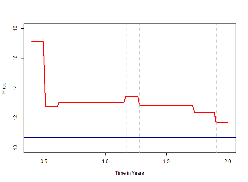
Figure 4 provides a section through the pricing surface for a strike . The found difference in the option priced between a Merton and a Bayesian Merton option price at the end of the observation period of two years still amounts to approximately 10% of the option’s price, which of course, is a significant deviation.
4 Conclusion
In the present work, we have given a systematic and mathematically rigorous account on Bayesian methods in option pricing for the case of the Black-Scholes and the Merton market. In particular, we proved the existence of equivalent martingale measures and market incompleteness for these Bayesian market models.
Bayesian corrections to option prices due to uncertainty in volatility estimates has been intensly studied in the context of time series models, see e.g. [6, 8, 9, 12, 14, 16, 21, 22]. We have shown that this concepts crucially depends on the observation frequency. In particular, as a consequence of Bayesian consistency, it is obsolete in the context of high frequency observations.
In contrast, Bayesian prices differ from non Bayesian ones even in the case of continuous observations, if Market models of exponential Lévy type are considered. The reason for this crucial difference to the BS-market lies in the fact that one can not increase the information on the jump distribution by simply increasing the observational frequency. The uncertainty on the jump distribution thus prevails over a span of time of several years and has a significant impact to option prices. Despite also this difference converges to zero in the observation time is sent to infinity, this mathematical result is not very relevant as the statistical properties of asset markets are certainly non stationary on a time scale of several years.
Despite Bayesian methods in asset pricing have been predominantly applied to volatility estimation in markets with Gaussian log-returns, we here suggest that Bayesian estimation and option pricing in exponential Lévy markets is an even more interesting application of the Bayesian approach in finance.
Appendix A The Saddle Point Method for Bayesian Consistency
Here we give a variant of the saddle point method that is tailored for the Bayesian consistency for option prices, see [3, 11] for comprehensive reviews on Bayesian consistency.
Let be some open region and let be some continuous, bounded and non negative function on such that . Let be continuous functions that are bounded from below such that uniformly on compact sets. Furthermore, assumes a unique global minimum, where it attains the value . Also, there exists a positive number and an open, bounded neighbourhood , , and such that for all we have . Finally we assume that .
Lemma A.1 (Saddle Point Method with Integrable Prior)
Let be as described above and let be a bounded and continuous function. Then,
| (28) |
Proof. We start the proof with the following bound on the convergence speed of the nominator to zero: Let , and let . As uniformly on compact sets, there exists a and a number such that for all and . Here is the ball around with radius . Thus, on . We now get
| (29) |
Here we also used that and thus the integral of over is positive.
Let next be arbitrary. Let as the minimum is unique and on with and as in the assumptions. If , with from the assumptions and sufficiently large such that on the compact set , we see that for such on . Consequently,
| (30) |
Combining this with (29), we obtain that
| (31) |
Therefore, applying (31) once for itself and one for replaced with one, we get from the fact that adding sequences converging to zero do not change the or the
| (32) | ||||
Likewise, we prove
| (33) |
As these inequalities (32) and (33) hold for arbitrary , we can take the supremum over in (32) and the infimum over in (33). By continuity of , we obtain as upper bound for the in (33) and as lower bound for the in (32) from which the convergence (28) follows.
The following Lemma deals with some modification of the previous, in order to deal with the case of a non integrable prior, like e.g. the non informative prior:
Lemma A.2 (Saddle Point Method with Non Integrable Prior)
Consider the situation in the beginning of the appendix, where however the prior is continuous and bounded, but not necessarily integrable. Let be a continuous function such that .
Suppose that, in case we replace the functions with the functions , these modified functions still fulfil the following condition: There exists a positive number , an open environment of and a number such that for all we have . Then, (28) still holds.
Proof. Note that on the left hand side of (28) we can replace with and with without changing the value of the integral. Obviously, also converges to uniformly on compact sets, as the continuous function is bounded on compact sets and thus uniformly on compact sets. We can thus apply Lemma A.1 to conclude.
References
- [1] D. Applebaum, Levy processes and stochastic calculus, Cambridge University Press, 2004.
- [2] F. Black and M. Scholes, The pricing of options and corporate liabilities, Journal of Political Economy 3, 1973.
- [3] T. Choi and R. V. Ramamoorthi, Remarks on consistency of posterior distributions, IMS Collections Vol. 3 (2008) 170-186.
- [4] R. and P. Tankov, Financial modelling with jump processes, Chapman and Hall/CRC, 2004
- [5] T. Darsinos and S. Satchell, Bayesian analysis of the Black-Scholes option price, Forecasting expected returns in the financial markets (2007): 117.
- [6] F. Delbaen, W. Schachermayer, A general version of the fundamental theorem of asset pricing, Mathematische Annalen, Springer-Verlag, 1994
- [7] P. Diakonis, D. Freedman, On the consistency of Bayes estimates, Ann. Statistics 14 (1) 1–26 (1986).
- [8] D. B. Flynn, S. D. Grose, G. M. Martin and Vance L. Martin, Pricing Australian and S& P200 options: A Bayesian approach based on generalized distributional forms, Aust. N. Z. J. Stat. 47(1), 2005, 101-117.
- [9] C. S. Forbes, G. M. Martin and J. Wright, Bayesian estimation of a stochastic volatility model using option and spot prices: application of a bivariate Kalman filter. No. 17/03. Monash University, Department of Econometrics and Business Statistics, 2003.
- [10] S. J. Frame, C. A. Ramezani, Bayesian estimation of asymmetric jump-diffusion processes, Ann. Finan. Econ. 09, 1450008 (2014)
- [11] S. Ghosal, A review of consistency and convergence of posterior distribution, Varanashi Symposium in Bayesian Inference, Banaras Hindu University. 1997.
- [12] H. Gzyl, E. ter Horst and S. W. Malone, Towards a Bayesian framework for option pricing, arXiv preprint cs/0610053 (2006)
- [13] P. R. Halmos, Measure theory, Springer 1950.
- [14] S. W. Ho, A. Lee and A. Marsden, Use of Bayesian estimates to determine the volatility parameter, Journ. of Risk and Financial Management 3 (2011) 74-96.
- [15] S. Iacus, Option pricing and estimation of financial models with R, Wiley & Sons 2011.
- [16] E. Jacquier and N. Polson, Bayesian econometrics in finance, Journal of Finance 58(3) (2003), 1269.
- [17] Kaila, R., The integrated volatility implied by option prices: A Bayesian approach, Dissertation Helsinki University of Technology Institute of Mathematics Research Reports, 2008.
- [18] R. Merton, Theory of rational option pricing, Bell J. of Economics 4 (1973) 141–183.
- [19] R. Merton, Option pricing when the underlying stock returns are discontinuous, J. Financial Economics 3 (1976) 125–144.
- [20] K.-I. Sato, Lvy Processes and Infinitely Divisible Distributions, Cambridge University Press, Cambridge, UK, 1999
- [21] Rachev, S. T., Hasu, J. S. J., Baghasheva, B. S. and Fabozzi, F. J.,Bayesian Methods in Finance, Wiley 2008.
- [22] J. V. K. Rombouts and L. Stentoft, Bayesian Option Pricing Using Mixed Normal Heteroskledasticity Models, Computational Statistics and Data analysis 76 (2014), 588–605.
- [23] W. Schachermayer, No arbitrage: On the work of David Kerps, Positivity 6 (2002) 359–368.